Estimating Above-Ground Biomass in Sub-Tropical Buffer Zone Community Forests, Nepal, Using Sentinel 2 Data


1
Graduate School of Agricultural and Life Sciences, University of Tokyo, 1-1 Yayoi, Bunkyo-Ku, Tokyo 113-8567, Japan
2
Institute for Water Studies, Dept. of Earth Sciences, University of the Western Cape, Private Bag X17, Bellville 7535, South Africa
*
Author to whom correspondence should be addressed.
Remote Sens. 2018, 10(4), 601; https://0-doi-org.brum.beds.ac.uk/10.3390/rs10040601
Submission received: 23 March 2018
/
Revised: 6 April 2018
/
Accepted: 11 April 2018
/
Published: 12 April 2018
(This article belongs to the Special Issue Biomass Remote Sensing in Forest Landscapes)
Abstract
:Accurate assessment of above-ground biomass (AGB) is important for the sustainable management of forests, especially buffer zone (areas within the protected area, where restrictions are placed upon resource use and special measure are undertaken to intensify the conservation value of protected area) areas with a high dependence on forest products. This study presents a new AGB estimation method and demonstrates the potential of medium-resolution Sentinel-2 Multi-Spectral Instrument (MSI) data application as an alternative to hyperspectral data in inaccessible regions. Sentinel-2 performance was evaluated for a buffer zone community forest in Parsa National Park, Nepal, using field-based AGB as a dependent variable, as well as spectral band values and spectral-derived vegetation indices as independent variables in the Random Forest (RF) algorithm. The 10-fold cross-validation was used to evaluate model effectiveness. The effect of the input variable number on AGB prediction was also investigated. The model using all extracted spectral information plus all derived spectral vegetation indices provided better AGB estimates (R2 = 0.81 and RMSE = 25.57 t ha−1). Incorporating the optimal subset of key variables did not improve model variance but reduced the error slightly. This result is explained by the technically-advanced nature of Sentinel-2, which includes fine spatial resolution (10, 20 m) and strategically-positioned bands (red-edge), conducted in flat topography with an advanced machine learning algorithm. However, assessing its transferability to other forest types with varying altitude would enable future performance and interpretability assessments of Sentinel-2.
1. Introduction
Accurate assessment of forest above-ground biomass (AGB) is important for the sustainable management of forests, particularly for buffer zone (BZ) areas whose dependence on forest products is high. In Nepal, the concept of the buffer zone was introduced with the intention of simultaneously alleviating the pressure from human development on conservation areas and addressing the socio-economic requirements of affected populations [1], thus aiming to resolve potential conflicts over forest product usage [2]. This, requires timely-based monitoring of available resource (biomass) and extraction magnitude. An assessment of AGB helps managers, foresters, and scientists to understand and monitor ecosystem responses and contributions to the global carbon cycle climate change and perform terrestrial carbon accounting [3,4,5,6]. Moreover, time series and repeated monitoring of the forest status can also provide a basis for decision-making and the sustainable use of forest resources with a view to introducing appropriate planning and conservation efforts. There are two basic approaches to forest biomass estimation: traditional field-based methods and remote sensing (RS) methods. There is no doubt that traditional methods are more accurate [6], but they are also time consuming, laborious, difficult to implement in inaccessible areas [6,7], and destructive in nature. Hence, research has favored remote sensing techniques since their inception. Although biomass cannot be directly measured from space, the use of spectrally-derived parameters from sensor reflectance (bands) enables increased biomass prediction accuracy when combined with field-based measurements [8]. For example, studies conducted by Chen et al. [9], Dube et al. [10], Dube et al. [11], Muinonen et al. [12], Rana et al. [13], and Shen et al. [14] utilized hyperspectral, LiDAR, and medium-resolution sensors with sufficient field data collection to estimate AGB. Although hyperspectral image data provides a wealth of information, it has some limitations, such as increased image costs, data volume, data redundancy, and data processing costs [15,16,17,18]. The limitation of using hyperspectral remote sensing technologies have also been discussed by Matheiu et al. [19] and have resulted in a shift towards the use of free and readily available broadband, including Landsat datasets and optical sensors, such as Sentinel-2 [20], which offer a large swath width, allowing timely and local to regional-scale AGB and carbon accounting [21,22,23].
In the past three decades, Landsat images have been mostly used for forest AGB estimation [11,24,25,26,27] mainly because of the freely-accessible long archive images with medium spatial resolution. However, one common problem is data saturation in Landsat imagery; an increase in biomass has been found to result in spectral saturation problems and this normally leads to under-estimation of biomass. For instance, a study conducted by Kasischke et al. [28] showed significant variations in the accuracy of biomass and vegetation indices (VIs) due to the saturation of spectral indices at higher biomass values. Likewise, Steininger [29] reported saturation of spectral values at approximately 150 t ha−1. Additionally, some studies have discredited the use of multi-spectral data in remote sensing analyses of plant biomass and biochemical properties [30]. The broad bandwidths and low spectral resolution of multi-spectral data are often cited as insensitive to the differences in plant characteristics [31,32,33,34]. Therefore, for accurate AGB estimation in complex sub-tropical areas such as Nepal, high-resolution data is a pre-requisite, especially if the saturation problem is to be overcome.
Sentinel-2 (equipped with a multi-spectral instrument, MSI) sensor, launched on 23 June 2015 by the European Space Agency (ESA), provides a significant improvement in spectral coverage, spatial resolution, and temporal frequency over the current generation of Landsat sensors [35]. It presents high potential for applications in land management, agricultural industry (food security), forestry (AGB) disaster control, and humanitarian relief operations [36]. The spectral configuration of Sentinel-2 is comparable to some commercial satellite data, such as Worldview-2 and RapidEye, because of the presence of the red-edge band, but is further improved by incorporating shortwave infrared bands (SWIR). The common characteristics of Sentinel-2 and commercial satellites only relate to the inclusion of the red-edge band, which is important for vegetation assessment and monitoring [37]. Sentinel-2 is a polar-orbiting sensor comprised of two satellites, each carrying an MSI characterized by a 290-km swath width, offering a multi-purpose design of 13 spectral bands traversing from visible and near-infrared (NIR) wavelengths to shortwave infra-red wavelengths at refined (10, 20 m) and coarse (60 m) spatial resolution. Furthermore, the presence of four bands within the red-edge region, centered at 705 (band 5), 740 (band 6), 783 (band 7), and 865 nm (band 8a) [38], gives the sensor high potential for mapping various vegetation characteristics. For instance, Ramoelo et al. [37] successfully demonstrated the potential of Sentinel-2 MSI red-edge bands for estimating grass nutrients. Similarly, Forkuor et al. [39] compared the use of Landsat 8 and Sentinel-2 data for mapping land use land cover (LULC) in rural Burkino Faso, where they concluded that the classification performance by Sentinel-2 red-edge bands alone produced better results than Landsat 8 and comparable results to other Sentinel-2 bands (i.e., visible, NIR, and SWIR).
Most previous studies have primarily focused on grass chlorophyll and nitrogen content [40], assessing rangeland quality [37], discriminating C3 and C4 grass species [38], and mapping and monitoring wetlands [41] and tree canopy cover [42], and have succeeded in showing the potential of Sentinel-2. However, to the best of our knowledge, its usefulness has not yet been evaluated for forest AGB estimation and mapping and neither evaluation has yet been conducted in the challenging and complex forest regions of Nepal, where saturation is a serious problem. It is in such locations that Sentinel-2, with its fine resolution and free/open access policy, can offer new opportunities for accurate and timely biomass estimation.
Minimal research has been conducted in Nepal with the application of RS technologies using hyperspectral sensors, especially for estimating AGB and, ultimately, carbon stocks. For example, Karna et al. [43] used WorldView-2 satellite images with small-footprint airborne LiDAR data to estimate tree carbon at the species level in a tropical forest in Nepal. Similarly, Baral [44] achieved 61% accuracy when predicting the carbon content of a sub-tropical forest in Central Nepal by integrating GeoEye and WorldView-2. Most Nepal studies have focused on tropical and sub-tropical forests, mainly because of the diversity of flora and fauna that is key to their ecosystems [45], but with few detailed ground-based quantifications of biomass [44]. Likewise, Murthy et al. [46] used LiDAR and field data to create a national forest inventory (2010–2014) for Nepal. These studies, however, generated good national-scale baseline data that can be used both for future monitoring and for REDD+ (Reducing Emissions from Deforestation and forest Degradation, plus other conservation activities) monitoring, reporting, and verification. Some attempts have also been made to explore the potential of coarse-resolution imagery for forest interpretation as well as for mapping forest cover and volume. For instance, Muinonen et al. [12] used k-nearest neighbor techniques to produce thematic maps of forest cover and total stand volume by combining Landsat TM (Thematic Mapper) and MODIS (MODerate resolution Imaging Spectroradiometer) data for the tropical forests of Western and Eastern Nepal.
To the best of our knowledge, this is the first attempt to conduct a study in the sub-tropical forest and integrate Sentinel-2 spectrally-derived indices to estimate AGB in a buffer zone community forest in Nepal by employing empirical modeling (Random Forest). The choice of Random Forest was based on prior studies, which have shown that the RF approach provides one of the best accuracies among empirical modeling. Strobl et al. [47] described the RF algorithm as an effective tool that can perform simple and complex regressions with modest parameter fine-tuning, resulting in greater prediction accuracy. One of the advantages of using RF is that it has the capacity to determine the importance of variables. For example, Karlson et al. [48] noted that incorporating an optimal subset of the most important variables improved the performance and interpretability of the RF model and should, therefore, be considered when RF is used to characterize the tree cover structure (e.g., tree canopy cover and AGB). Variable selection allows the prediction algorithm to focus its attention on relevant variables while ignoring the contribution of irrelevant variables that can be misleading [49]. By reducing the number of input variables, the model is faster and less prone to overfitting. It also allows a better understanding of the underlying processes that generated the data [50]. The main aim of this study is, therefore, to investigate the performance of spectrally-derived indices using Sentinel-2 MSI combined with field measurements for estimating AGB in the sub-tropical buffer zone community forest of Parsa National Park, Nepal. Additionally, variable selection is considered as a key step required to generate the smallest subset of input variables in the RF algorithm.
2. Materials and Methods
2.1. Study Area
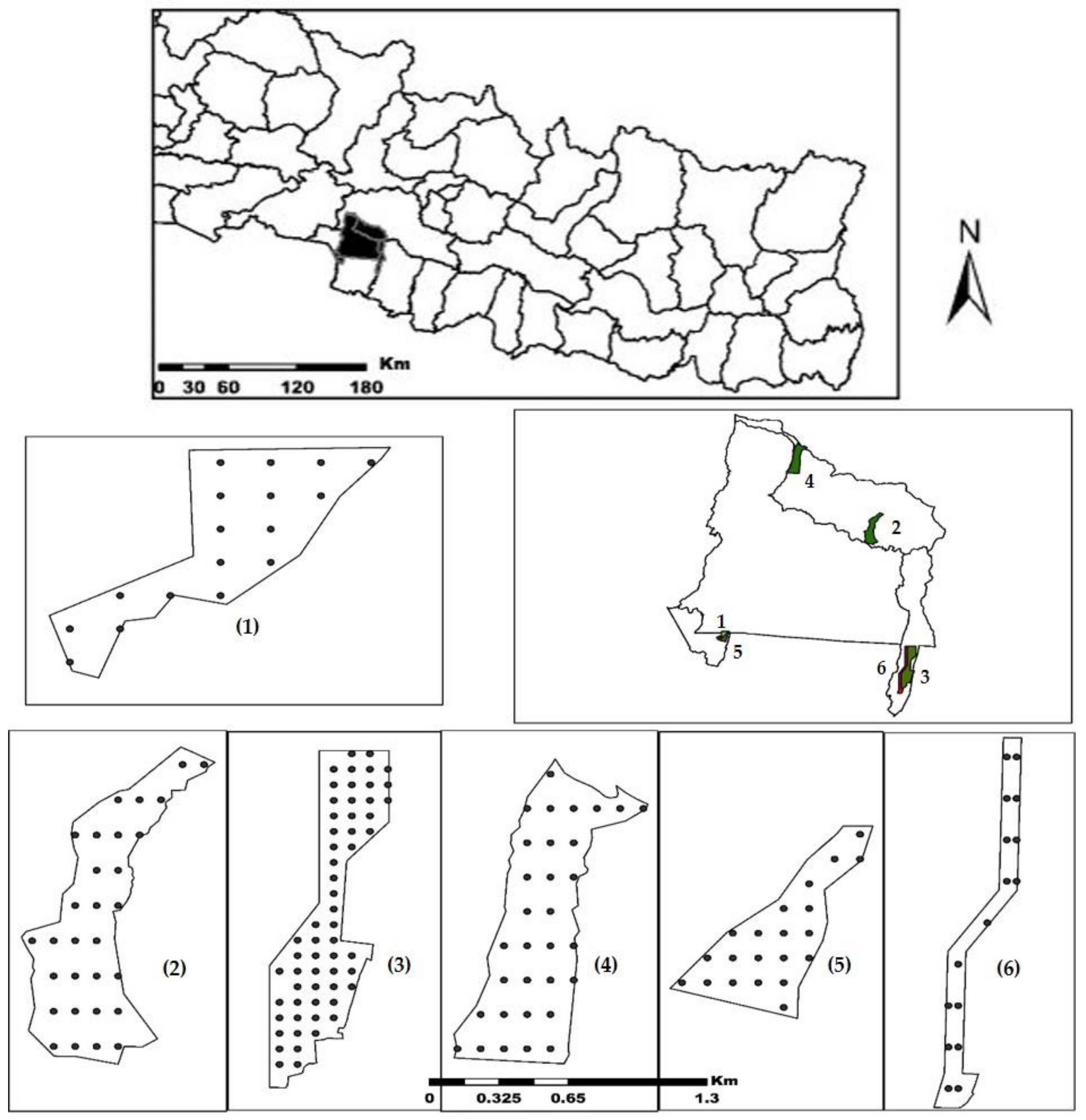
The study area (Figure 1) is a protected area in Parsa National Park, situated in the Central-Southern part of Nepal. Six buffer zone community forests (BZCFs) in this park were selected based on the renewed work plan of the forest user group and available GPS boundaries. Geographically, the reserve lies between latitude 27°28′0′′N and longitude 84°20′0′′E. The topography of the study area is flat with minor slope variations. The area is characterized by a sub-tropical climate, with an annual mean temperature of 24.5 °C and precipitation of 1908 mm recorded during 1981–2010; however, the winters are cold and foggy. The vegetation is mainly dominated by Shorea robusta (vernacular name: Sal). As the elevation increases, it is replaced by Pinus roxburghii. All the selected natural forest areas were later handed over to the community for protection and management.
2.2. Sampling Strategy and Field Data Collection
Of the six selected community forest areas, four BZCFs (Radha Krishna, Mushaharnimae, Shrijana, and Ratomate) were chosen for the establishment of temporary circular plots 500 m2 (r = 12.62 m). These plots were randomly generated, considering the flat topographical structure of the study area, in ArcGIS version 10.3 (ESRI, Redlands, CA, USA) The forest types and species distributions are almost equal; thus, we chose to vary the species samples between plots considering the size of the forest in order to minimize the required time and labor. The forest size varied from 66 ha to 650 ha. Altogether, 113 plots were sampled. Some of the plots within the boundary of the forest were considered as outliers and discarded from the measurement. Two forest datasets (Janahit and Jyamire) were provided by the park. The methodology we adopted for sampling and sizing of the plots was the same as for these datasets. The data collection date for the two forests was only a few months difference from the date of the remaining data collection (24 February to 12 March 2016); hence, the biomass amount would not be substantially different.
All the trees inside the circular plot were measured. Forest parameters, namely the diameter at breast height (DBH) ≥ 5 cm (1.3 m above the ground) and tree height (H), were measured using DBH measuring tape (Yamayo measuring tools Co. Ltd., Tokyo, Japan) and a Hypsometer vertex laser instrument (Laser technology, Inc., Colorado, USA) respectively. Additionally, the species name of each tree was noted in all 113 plots.
Estimation of Plot-Based AGB
Tree biomass was estimated using an existing species-specific allometric equation developed by Chave et al. [51], which is based on climate and forest types. Species with their default specific values (ρ) given by Chaturvedi and Khanna [52] were used to calculate tree level biomass. In the absence of specific values, a general value (ρ = 0.674) was used as recommended. Individual biomass for all trees within the plot was calculated following Equation (1) and then aggregated to obtain individual plot-level AGB. Then, it was standardized to tonnes per hectare (t ha–1). Tree-level AGB was estimated using the following equation:
where AGB is the above-ground biomass (kg); ρ is the specific gravity (g cm–3); D is the diameter at breast height (cm); and H is the tree height (m) and the constant 0.0509 was obtained from the literature [51].
AGB = 0.0509 × ρD2 H
2.3. Satellite Image Acquisition and Data Processing
Single tile standard Sentinel-2A Level-1C (L1C) product acquired on 28 December 2015 was downloaded from THE USGS Earth Explorer. This is the only date a cloud-free image could be obtained as dates close to those of the field survey exhibited cloud and haze even after pre-processing. This product is an ortho-image in UTM/WGS 84, 45N projection, with per-pixel radiometric measurements provided for top-of-atmosphere (TOA) reflectance. The data is acquired in 13 spectral bands extending through visible, near-infrared (NIR), red-edge, and shortwave infra-red (SWIR) wavelengths at 10, 20, and 60 m spatial resolution. In this research, bands 1, 9, and 10 were excluded as they are used to detect atmospheric features. The image was transformed from radiance to surface reflectance by applying the dark object subtraction (DOS) method using the semi-automatic classification plugin (SCP) in QGIS version 2.14 software (QGIS development team, Berne, Switzerland). This removed the darkest pixels from each band that might be affected by atmospheric scattering [53]. Moreover, the red-edge bands and SWIR bands were resampled to 10-m resolution using ArcGIS version 10.4 (ESRI, Redlands, CA, USA) to determine the advantage of higher resolution.
2.4. Variables for Forest AGB Prediction
To test the applicability of the Sentinel-2 MSI sensor for estimating community forest AGB, raw bands and vegetation indices (VIs) were used. Spectra values were generated by creating a signature in ENVI classic version 5.3 and averaged for each plot. Thereafter, they were used for calculating the selected vegetation indices. The selection of vegetation indices (VIs) was based on their performance in forest biophysical studies in previous studies [38,54,55]. Table 1 shows the raw bands and specific calculated broad band, narrow band, light use efficiency, and dry or senescent carbon vegetation indices used in this study to perform spatial modeling. Altogether, the number of input data used as independent variables were n = 24, including the selected bands and VIs.
2.5. Statistical Analysis
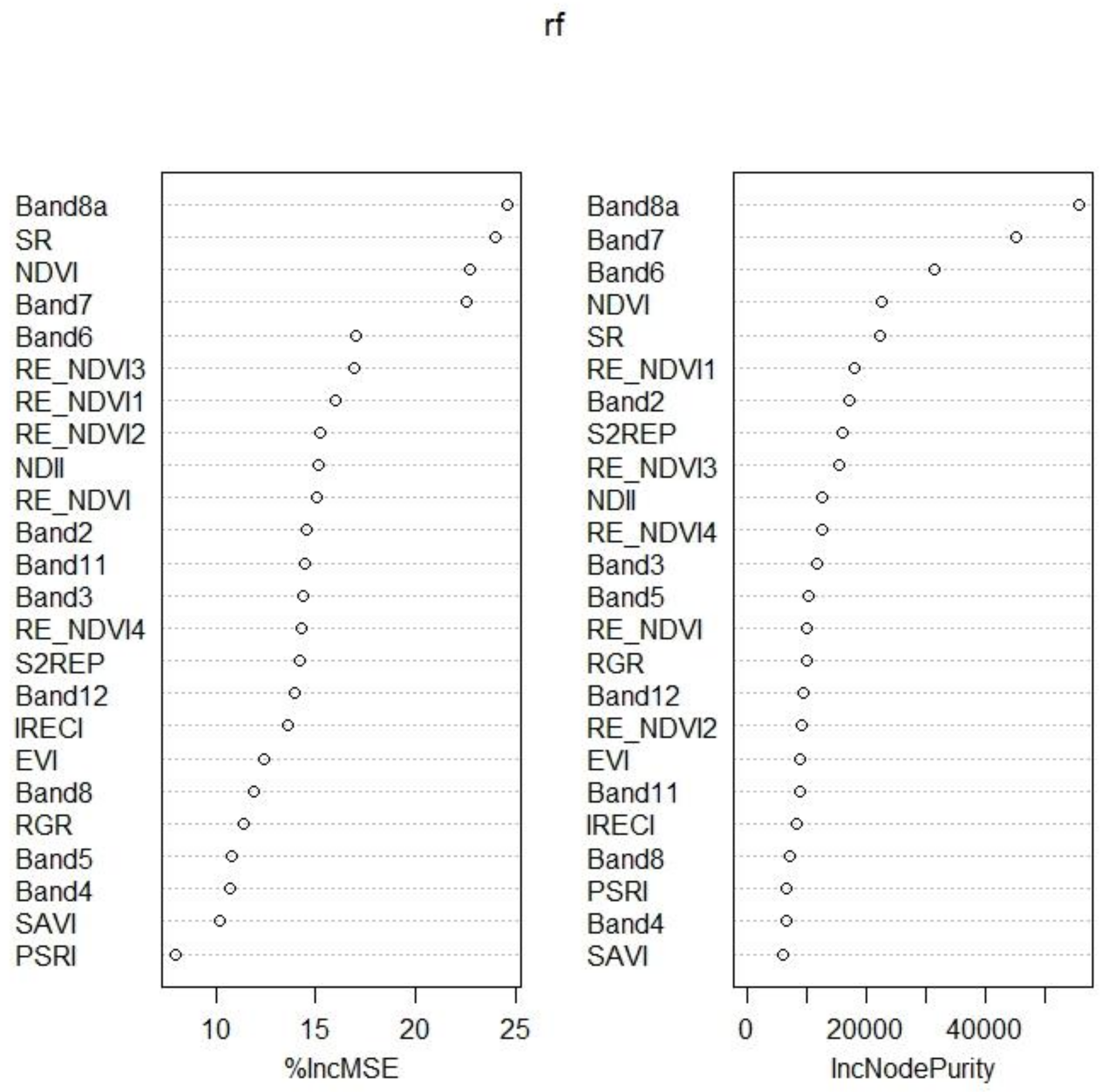
Estimation of forest AGB using Sentinel-2-derived information was based on the extension of a tree-based model called Random Forest. A detailed description of the basic theory behind the model is provided by Breiman [68]; it has been successfully applied to AGB estimation coupled with remote sensing and field data in different forest bio-physical contexts. In this algorithm, decision trees are generated to the maximum extent without pruning using a randomly-selected two thirds of the samples as training data with bootstrapping (re-sampling the data many times with replacement), which strengthens the flexibility by aggregating the prediction across individual trees to make a final prediction. The rest of the data, i.e., the remaining third, is called OOB data (out-of-bag), is not seen by the model, and is used as validation samples to estimate the model errors [69]. Furthermore, at each node of the decision tree, selection of the features for modeling is also stochastic, making the approach immune to the problem of over-fitting [68]. Therefore, there are two important parameters, namely mtry, which is denoted as the number of variables available for splitting at each node of the tree, and ntree, which is the number of trees adjusted to achieve a desirable prediction. These two parameters (mrty and ntree) were optimized to achieve a desirable prediction (selecting the lowest RMSE) [68,70,71]. The default value for ntree is 500 and that for mtry is 1/3 of the total number of variables used in the model. In our case, optimization of ntree for the full predictor variable resulted in a value of 1600, whereas mrty was 12, which explained the variables optimally. Another advantage of RF is that it calculates the relevance of the predictor variables (important variable selection), assigning a score that depends on changes in the error when a particular variable is varied (%IncMSE refers to the effect of the variable when it is removed from the model and IncNodePurity describes how pure the node is when that variable is in the model). The larger the effect of a variable, the more importance is assigned to that variable [72]. Taking this into account, all the remote sensing-generated variables were used for AGB estimation and the IncNodePurity measure was used to determine the variable importance. To identify whether a smaller set of the variable would improve model performance, ntree and mtry were tested in the range of 200 to 1100 and 1 to 9, respectively, which explained the variables optimally. The regression process was completed in the open-access R statistical software 3.4 version [68] using the “randomForest” package.
Although RF is a powerful and accurate method used in machine learning, cross-validation was performed to avoid overfitting of the model. The 10-fold cross-validation was used to assess the estimation of AGB. In addition, validation measures, namely the coefficient of determination (R2), the root mean square error (RMSE), and the relative RMSE (relRMSE) between the simulated AGB and the field-measured AGB, were calculated to assess the estimation performance because this approach measures the percentage of the variation explained by the regression model [26]:
where yi is the biomass calculated in the field; is the predicted biomass value; and i represents each of the predictor variables included in the summation process (n = 24), and:
where represents the mean AGB value from the field measurements.
3. Results
3.1. Field-Based AGB Estimates
Table 2 shows the descriptive statistics of plot-level AGB. Forest stand parameters (DBH and Ht) measured for individual trees within the circular plot were aggregated to generate plot-level AGB for all sampling plots in the six forests. High biomass was observed for Jyamire BZCF (304.19 t ha–1) while Shrijana BZCF (30.34 t ha–1) had the lowest field-measured biomass. The average AGB previously estimated for the Terai region of Nepal was 196.18 t ha–1 [45]. In this study, the average AGB for all six forests was 153.04 t ha–1, which is lower than the value determined by [45].
Altogether, 34 species were recorded in the field and eight species were unidentified. Though many species were recorded, there were only five dominant species (Shorea robusta, Mallotus philipensis, Anogeissus laifolia, Daubanga grandiflora, and Casearia graveolens); Shorea robusta was dominant over the entire study area.
3.2. RF Performance Based on All Variables and Important Variable
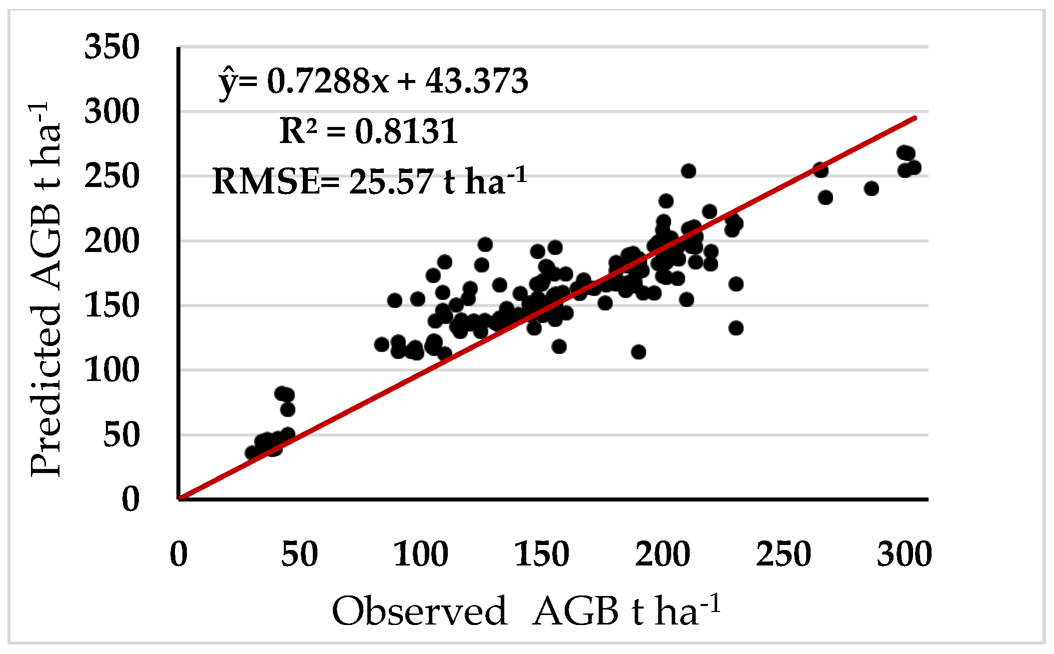
Considering the potential of the RF algorithm for predicting forest biomass, the RF model with all input variables (n = 24) produced a plausible result according to the percentage of variables explained by the model (R2 = 0.81 and RMSE = 25.22 t ha−1). The number of trees ntrees and mtry was adjusted to generate a better prediction result. This fine-tuning offered by the RF algorithm yielded optimal ntrees and mtry values of 1600 and 12, respectively, which produced the lowest RMSE. The relationship between observed and predicted biomass using all variables is shown in Figure 2.
3.3. Variable Importance
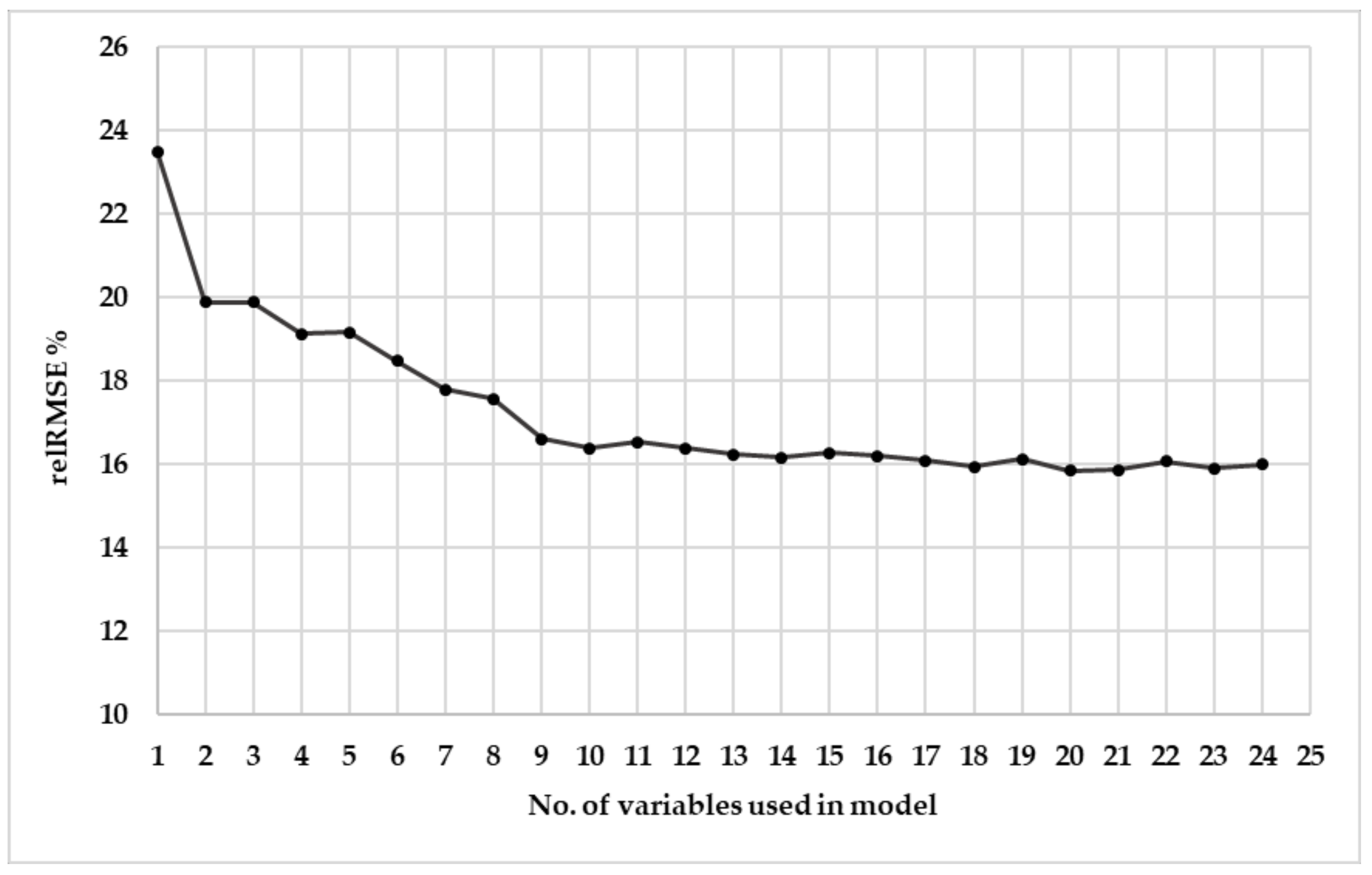
RF also calculates the relevance of the input variables using %IncMSE and IncNodePurity (Figure 3). The variable selection method used in this study identified the smallest subset of predictor variables in the model. Using the variable importance chart generated by variable important features as a reference, progressive backward feature elimination (removing the least important) did not substantially improve model performance (Figure 4). Removal of the six least important variables from the model resulted in similar R2 values (0.81); however, there were inconsistencies in the RMSE value, in that slight increases or decreases were observed when the variables were progressively removed from the model (Table 3). Likewise, continuing the procedure further did not improve model performance; on the contrary, the coefficient of determination decreased, thereby increasing the RMSE value of the model. It is notable that the RMSE generally increased as the least important variables were progressively discarded, an approach which fails to further identify the smallest number of predictor variables. Thus, the full set of predictor variables that yielded the highest R2 (0.81) and low RMSE (25.32 t ha−1) values were considered in the final RF algorithm to predict the AGB of the community forest.
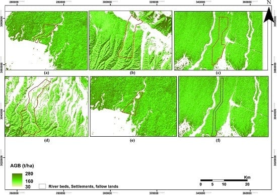
3.4. AGB Mapping Using Sentinel-2 MSI Data
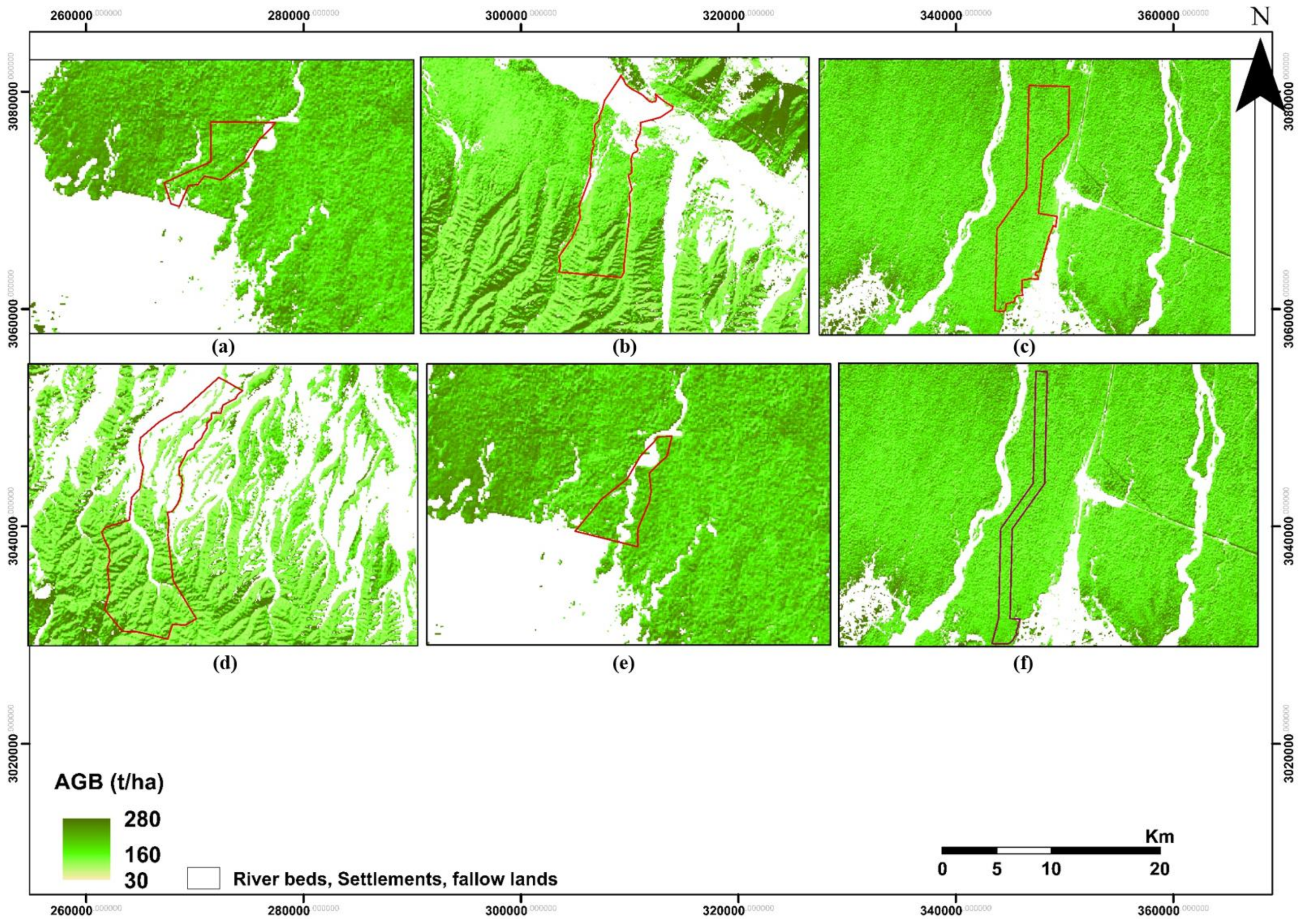
An AGB map was produced using the best predictor variables from the final model generated by the RF algorithm. The choice of Sentinel-2 spectral bands and spectral-derived VIs for producing biomass estimates was based on the fact that it produced overall plausible and strongly-explained variable values, with R2 = 0.81, a low root mean square error, and a low relative root mean square error. Figure 5 shows distinct AGB spatial distribution patterns within the selected community forest. The average predicted forest biomass was 160 t ha−1, the minimum biomass estimate was 35.42 t ha−1, and the maximum estimate was 276.92 t ha−1. Overall, the model underestimated the high observed biomass, but overestimated low observed biomass.
4. Discussion
The goal of this study was to examine the potential of the Sentinel-2 MSI sensor for estimating natural forest biomass in buffer zone areas of Parsa National Park using the random forest algorithm. This study, therefore, aimed to investigate whether the refined spatial resolution (10 m) and greater band availability (red-edge) could improve the quantification of above-ground biomass and provide a better alternative for hyperspectral resource-constrained regions.
Quantitative determination and mapping of forest AGB using remote-sensing techniques, especially using medium-resolution imagery, is a challenging task for complex and dense forest stands [73]. For instance, Muukkonen and Heiskanen [74] showed that the shadows are inversely related to the reflectance of spectral bands as biomass increases. Similarly, other studies have shown significant variations in modeling between biomass and vegetation indices, due to the saturation tendency of spectral indices when biomass increases; for example, a study conducted by Steininger [29] observed saturation at approximately 150 t ha−1. However, many studies have indicated the successful application of optical remote sensing data and the varying effectiveness and efficiency of using sensors with strategically positioned bands (red-edge bands), such as Sentinel-2, in forest biophysical studies to overcome this problem. For instance, Sibanda et al. [20] compared Sentinel-2 MSI and Landsat 8 OLI estimations of the AGB of grasses treated with different fertilizer treatments. Their results showed better performance by Sentinel-2 derived models, with an R2 value of 0.81 and an RMSE of prediction (RMSEP) value of 1.07 kg m−1. Landsat 8 OLI yielded a slightly lower R2 value of 0.76 and an RMSEP value of 1.15 kg m−1. This result is similar to the findings of this study, where the R2 and RMSE values evaluating the variance explained by the RF algorithm were 0.81 and 25.57 t ha−1, respectively, using the full set of predictor variables (Table 1), and the important variable selection process decreased the RMSE to 25.32 t ha−1 for 20 input variables. The good performance achieved using spectral and spectral-derived indices from Sentinel-2 can be attributed to its advanced sensor design, which consists of two satellites, each carrying an MSI characterized by a 290-km swath width, and is potentially suitable for vegetation biophysical parameter (leaf area index, nitrogen, and chlorophyll), agriculture, and forest monitoring. This sensor offers a multipurpose design of 13 spectral bands from visible and near infrared up to shortwave infrared [20] wavelengths, offering a refined spatial resolution of 10 m and 20 m, allowing improved and more accurate spatial representation of vegetation. As described in Section 2, resampling of 20-m resolution bands (5, 6, 7, 8a, 11, and 12) to 10 m increases the variation in terms of pixel values per plot considering the sample plot size [75]. Moreover, there are four strategically-positioned bands (novel bands) that are critical for vegetation mapping when compared to traditional broadband images, such as Landsat Thematic Mapper and Enhanced Thematic Mapper, which increases the potential area for vegetation mapping [10,38].
Shoko and Mutanga [38] demonstrated the superior ability of Sentinel-2 to classify C3 and C4 grasses in comparison with Worldview-2 and Landsat 8 OLI sensors through a discriminant analysis using three datasets of bands, indices, and a combination of both. The classification accuracies reached 90.36% (using bands), 85.54% (using indices), and 88.61% (using bands and indices), which were comparable with Worldview-2 (95.69%, 86.02%, and 87.09%, respectively), and better than Landsat 8 OLI (75.26%, 82.79%, and 82.79%, respectively). These results confirm the reported potential of strategic positioning, as well as additional bands, for enhancing the ability of the sensor to discriminate species. Similarly, a study by Ramoelo et al. [37] reported the importance of the red-edge band and SWIR bands in estimating nitrogen concentration in grass, whereas Laurin et al. [76] identified the SWIR as carrying water, nitrogen, and carbon (lignin, cellulose) content information, which aids in grass discrimination. This highlights why Sentinel-2-derived predictor variables are better for predicting forest biomass. Further, selection of the most important variables offered by the RF algorithm in this study also proved that the red-edge bands contribute to the optimal variables to the RF model (Figure 3). Additionally, the technically-advanced nature of the sensor, such as the 1C level where radiometric and geometric correction (including orthorectification and spatial registration) are performed and top-of-atmosphere (TOA) is calculated (ESA-31) favorably for the flat topography, ensures that it does not require additional terrain correction processes. It should be noted that all Sentinel-2 products are systematically processed to level 1C, a unique level released for users from the European Space Agency (ESA) [77].
Further, another possible reason for the improved performance of the regression might have been the combination of VIs derived from the red-edge bands. For example, Adam et al. [78] stated that using VIs can partially reduce the impacts of environmental conditions and shadows on reflectance, thus improving the correlation between AGB and VIs, especially in those sites with complex vegetation stand structures. Additionally, Laurin et al. [76] suggested that the use of the red-edge-derived VIs helps mitigate the saturation issue.
Finally, improved AGB estimation using 10-m resolution Sentinel-2 MSI sensor-derived vegetation indices can be linked with the capability of the machine learning algorithm. Previous research has precisely demonstrated the capabilities of advanced machine learning techniques, such as RF and stochastic gradient boosting, related to simplifying and increasing AGB estimation accuracy compared to linear modeling [5,10,11,78]. The advantage of non-parametric algorithms is that they do not make any assumptions about the form of the model and the distribution of input data, which makes it possible to effectively describe the non-linear relationship between forest AGB and remote sensing data [79]. One of the greatest strengths of RF regression ensembles is their robustness in handling inaccurate training data as they are less sensitive to data noise, outliers, and missing or unbalanced datasets [80]. The use of percentIncMSE and IncNodePurity to rank all predictor variables by their capacity to predict forest AGB did not improve the percentage of variables explained (R2), but lowered the root mean square error from 25.57 for the full set of predictor variables to 25.32 t ha−1 with the exclusion of the least important variable from the model. A plausible explanation for the improved performance of the reduced model is that the RF mechanism succeeded in blocking the influence of noisy predictor variables [78]. In a previous study, the authors reported a similarly strong performance of the RF model when estimating the AGB of a sub-tropical forest in Northwest Zhejiang Province, China [81]. Moreover, a study by Karlson et al. [48] showed the effectiveness of Landsat 8 OLI for estimating tree canopy cover (TCC) and AGB in Sudano-Sahelian woodland landscapes using the RF algorithm. They concluded that the best model for TCC had R2 and RMSE values of 0.77 and 8.9, whereas the model for AGB had R2 and RMSE values of 0.57 and 17.6 t ha−1, respectively. Mutanga et al. [82] explored the possibility of estimating biomass in a densely vegetated wetland area using NDVI computed from WorldView-2 using the RF algorithm and stepwise multiple linear regression. The RF algorithm and three NDVIs computed from the red-edge and NIR bands yielded an RMSEP value of 0.441 kg m−2 (12.9% of observed mean biomass) compared to the stepwise multiple linear regression, which produced an RMSEP value of 0.546 kg m−2 (15.9% of the observed mean biomass).
However, it is important to note that previous research using remote sensing has reported various results for different modeling approaches to the empirical estimation of AGB using remote sensing and field data. It is difficult to conclude outright that one is superior to another; therefore, each application requires an assessment of the optical bands and indices used to estimate biomass from the spectral relationship [6,24,28], with particular consideration of the forest type, topographical features, and objectives of the study. Thus, the effectiveness and robustness of the RF ensemble in variable selection based on remotely-sensed data still requires further research. Additional work should also evaluate the potential of freely accessible fine spatial resolution Sentinel-2 data for mapping and understanding forest biomass prediction, in order to fill the gaps in our knowledge related to Sentinel-2 and different types of forest AGB relationships.
Our results demonstrate that the RF algorithm is a useful and robust method for estimating AGB in sub-tropical deciduous forests with the fine spatial resolution (10 m) offered by Sentinel-2 data combined with spectrally-derived indices and field observations. The ability to handle non-linearity, automatically produce accuracy assessments, and measure the importance of variables makes RF an effective algorithm. Additionally, when the parameters are fine-tuned, RF is highly likely to show better performance through lowering the model error.
Additionally, this study attempts to highlight the forest condition in the buffer zone area through the means of AGB, where it is supposed to be utilized in a sustainable manner by reducing pressure in the core area. It is worth comparing the AGB between these two forests (community forest and protected forest) in future work. We assume this helps to provide a clearer picture of the role of the community on the forestry sector in Nepal.
5. Conclusions
This study investigates the performance of the RF algorithm in predicting forest AGB in BZCFs of Parsa National Park, Nepal, using fine spatial resolution Sentinel-2 MSI data with strategically-positioned spectral bands, which are missing from broadband multispectral sensors.
We conclude that:
- Sentinel-2 data effectively predicted the above-ground biomass of the sub-tropical forests, with an R2 value of 0.81 and an RMSE value of 25.57 t ha−1.
- The RF model selection of important variables did not improve the variance explained by the model (R2), but decreased the model performance error (RMSE) from 25.57 to 25.32 t ha−1.
- Technical improvements in the Sentinel-2 MSI sensor at fine medium resolution (10 and 20 m) have the potential to enable satisfactory predictions of biomass in areas of sub-tropical forest with flat terrain.
The results of this study suggest further work in the near future, such as the applicability of this data to other physiographical vegetation zones in different environments, should be evaluated using spectral texture indices. Additionally, we suggest applying the RF regression model to a very large sample size to determine if this reduces the estimation error. Remote sensing provides a non-destructive, effective, and efficient way of detecting information on forest biomass and carbon sequestration data. Sentinel-2 data offers wider accessibility, more spectral bands, and finer resolution than commercial moderate resolution datasets (e.g., ASTER) when used in conjunction with concurrent and robust machine learning approaches, e.g., the RF algorithm. Therefore, it represents a critical tool for assessing and monitoring forest biomass at local and regional scales in resource-constrained areas. This valuable sensor should be further exploited in studying the sensitivity measurements and vegetation properties of Nepal’s forests and recognizing it as an alternative sensor for areas where hyperspectral data is scarce.
Acknowledgments
This study used the Parsa National Park dataset comprising two forest observation datasets. We thank the Department of National Parks and Wildlife Conservation–Nepal for allowing the permit to collect our field data, and all the Community Forest User’s Group, local members, Amrit Science Campus, and especially forest guards for their kind support and assistance during the field phase. Additionally, we thank the reviewers for their valuable comments.
Author Contributions
Santa Pandit designed the study, analyzed the data, and wrote the paper. Satoshi Tsuyuki and Timothy Dube helped to review the manuscript.
Conflicts of Interest
The authors declare no conflict of interest.
References
- Ebregt, A.; Greve, P.D. Buffer Zones and Their Management: Policy and Best Practices for Terrestrial Ecosystems in Developing Countries; Theme Studies Series; National Reference Centre for Nature Management: Wageningen, The Netherlands, 2000. [Google Scholar]
- Stræde, S.; Treue, T. Beyond buffer zone protection: A comparative study of park and buffer zone products’ importance to villagers living inside Royal Chitwan National Park and to villagers living in its buffer zone. J. Environ. Manag. 2006, 78, 251–267. [Google Scholar] [CrossRef] [PubMed]
- Chinembiri, T.S.; Bronsveld, M.C.; Rossiter, D.G.; Dube, T. The precision of C stock estimation in the Ludhikola watershed using model-based and design-based approaches. Nat. Res. Res. 2013, 22, 297–309. [Google Scholar] [CrossRef]
- Gara, T.; Murwira, A.; Chivhenge, E.; Dube, T.; Bangira, T. Estimating wood volume from canopy area in deciduous woodlands of Zimbabwe. South. For. 2014, 76, 237–244. [Google Scholar] [CrossRef]
- Güneralp, I.; Filippi, A.M.; Randall, J. Estimation of floodplain aboveground biomass using multispectral remote sensing and nonparametric modeling. Int. J. Appl. Earth Obs. Geoinf. 2014, 33, 119–126. [Google Scholar] [CrossRef]
- Lu, D. The potential and challenges of remote sensing-based biomass estimation. Int. J. Remote Sens. 2006, 27, 1297–1328. [Google Scholar] [CrossRef]
- Henry, M.; Picard, N.; Trotta, C.; Manlay, R.J.; Valentini, R.; Bernoux, M.; Saint-André, L. Estimating tree biomass of Sub-Saharan African forests: A review of available allometric equations. Silva Fenn. 2011, 45, 477–569. [Google Scholar] [CrossRef]
- Dong, J.; Kaufmann, R.K.; Myneni, R.B.; Tucker, C.J.; Kauppi, P.E.; Liski, J.; Buermann, W.; Alexeyev, V.; Hughes, M.K. Remote Sensing estimates of boreal and temperate forest woody biomass: Carbon pools, sources, and sinks. Remote Sens. Environ. 2003, 84, 393–410. [Google Scholar] [CrossRef]
- Chen, J.; Gu, S.; Shen, M.; Tang, Y.; Matsushita, B. Estimating aboveground biomass of grassland having a high canopy cover; an exploratory analysis of in situ hyperspectral data. Int. J. Remote Sens. 2009, 30, 6497–6515. [Google Scholar] [CrossRef]
- Dube, T.; Mutanga, O.; Elhadi, A.; Ismail, R. Intra-and-inter species biomass prediction in a plantation forest: Testing the utility of high spatial resolution space borne multispectral RapidEye sensor and advance machine learning algorithms. Remote Sens. 2014, 14, 15348–15370. [Google Scholar] [CrossRef] [PubMed]
- Dube, T.; Mutanga, O. Evaluating the utility of the medium-spatial resolution Landsat 8 multi-spectral sensor in quantifying aboveground biomass in Umgeni catchment, South Africa. ISPRS J. Photogramm. Remote Sens. 2015, 101, 36–46. [Google Scholar] [CrossRef]
- Muinonen, E.; Parikka, H.; Pokharel, Y.P.; Shrestha, S.M.; Eerikäinen, K. Utilizing a multi-source forest inventory technique, MODIS data and Landsat TM images in the production of forest cover and volume maps for the Terai Physiographic Zone in Nepal. Remote Sens. 2012, 4, 3920–3947. [Google Scholar] [CrossRef]
- Rana, P.; Korhonen, L.; Gautam, B.; Tokola, T. Effect of field plot location on estimating tropical forest above ground biomass in Nepal using airborne laser scanning data. ISPRS J. Photogramm. Remote Sens. 2014, 94, 55–62. [Google Scholar] [CrossRef]
- Shen, W.; Li, M.; Huang, C.; Wei, A. Quantifying live aboveground biomass and forest disturbance of mountainous natural and plantation forests in Northern Guangdong, China, based on Multi-temporal Landsat, PALSAR and field plot data. Remote Sens. 2016, 8, 595. [Google Scholar] [CrossRef]
- Bajcsy, P.; Groves, P. Methodology for hyperspectral band selection. Photogramm. Eng. Remote Sens. 2004, 70, 793–802. [Google Scholar] [CrossRef]
- Govender, M.; Chetty, K.; Bulcock, H. A review of hyperspectral remote sensing and its application in vegetation and water resource studies. Water S. Afr. 2007, 33, 145–152. [Google Scholar] [CrossRef]
- Lefsky, M.A.; Cohen, W.B.; Spies, T.A. An evaluation of alternative remote sensing products for forest inventory, monitoring, and mapping of Douglas-fir forests in western Oregon. Can. J. For. Res. 2001, 31, 78–87. [Google Scholar] [CrossRef]
- Plaza, A.; Benediktsson, J.A.; Boardman, J.W.; Brazile, J.; Bruzzone, L.; Camps-Valls, G.; Chanussot, J.; Fauvel, M.; Gamba, P.; Gualtieri, A.; et al. Recent advances in techniques for hyperspectral image processing. Remote Sens. Environ. 2009, 113, 110–122. [Google Scholar] [CrossRef]
- Mathieu, R.; Naidoo, L.; Cho, M.A.; Leblon, B.; Main, R.; Wessels, K.; Asner, G.P.; Buckely, J.; Aardt, J.V.; Erasmus, B.F.N.; et al. Toward structural assessment of semi-arid African savannahs and woodlands: The potential of multitemporal polarimetric RADARSAT-2 fine beam images. Remote Sens. Environ. 2013, 138, 215–231. [Google Scholar] [CrossRef]
- Sibanda, M.; Mutanga, O.; Rouget, M. Examining the potential of Sentinel-2 MSI spectral resolution in quantifying above ground biomass across different fertilizer treatments. ISPRS J. Photogramm. Remote Sens. 2015, 110, 55–65. [Google Scholar] [CrossRef]
- Gibbs, H.K.; Brown, S.; Niles, J.O.; Foley, J.A. Monitoring and estimating tropical forest carbon stocks: Making REDD a reality. Environ. Res. Lett. 2007, 2, 045023. [Google Scholar] [CrossRef]
- Hall, F.G.; Bergen, K.; Blair, J.B.; Dubayah, R.; Houghton, R.; Hurtt, G.; Kellndorfer, J.; Lefsky, M.; Ranson, J.; Saatchi, S.; et al. Characterizing 3D vegetation structure from space; mission requirements. Remote Sens. Environ. 2011, 115, 2753–2775. [Google Scholar] [CrossRef]
- Laurin, G.V.; Chen, Q.; Lindsell, J.A.; Coomes, D.A.; Del Frate, F.; Guerriero, L.; Pirotti, F.; Valentini, R. Aboveground biomass estimation in an African tropical forest with lidar and hyperspectral data. ISPRS J. Photogramm. Remote Sens. 2014, 89, 49–58. [Google Scholar] [CrossRef]
- Foody, G.M.; Boyd, D.S.; Cutler, M.E. Predictive relations of tropical forest biomass from Landsat TM data and their transferability between regions. Remote Sens. Environ. 2003, 85, 463–474. [Google Scholar] [CrossRef]
- Hall, R.J.; Skakun, R.S.; Arsenault, E.J.; Case, B.S. Modeling forest stand structure attributes using Landsat ETM+ data: Application of mapping of aboveground biomass and stand volume. For. Ecol. Manag. 2006, 225, 378–390. [Google Scholar] [CrossRef]
- Lu, D. Aboveground biomass estimation using Landsat TM data in the Brazilian Amazon. Int. J. Remote Sens. 2005, 26, 2509–2525. [Google Scholar] [CrossRef]
- Powell, S.L.; Cohen, W.B.; Healey, S.P.; Kennedy, R.E.; Moisen, G.G.; Pierce, K.B.; Ohmann, J.L. Quantification of live aboveground forest biomass dynamics with Landsat time-series and field inventory data: A comparison of empirical modeling approaches. Remote Sens. Environ. 2010, 114, 1053–1068. [Google Scholar] [CrossRef]
- Kasischke, E.S.; Goetz, S.; Hansen, M.C.; Ozdogan, M.; Rogan, J.; Ustin, S.L.; Woodcock, C.E. Remote Sensing for Natural Resource Management and Environmental Monitoring, 3rd ed.; John and Wiley and Sons, Inc.: Hoboken, NJ, USA, 2014. [Google Scholar]
- Steininger, M.K. Satellite estimation of tropical secondary forest above-ground biomass: Data from Brazil and Bolivia. Int. J. Remote Sens. 2000, 21, 1139–1157. [Google Scholar] [CrossRef]
- Broge, N.H.; Mortensen, J.V. Deriving green crop area index and canopy chlorophyll density of winter wheat from spectral reflectance data. Remote Sens. Environ. 2002, 81, 45–57. [Google Scholar] [CrossRef]
- Broge, N.H.; Leblanc, E. Comparing prediction power and stability of broadband and hyperspectral vegetation indices for estimation of green leaf area index and canopy chlorophyll density. Remote Sens. Environ. 2001, 76, 156–172. [Google Scholar] [CrossRef]
- Curran, P.J. Imaging spectrometry for ecological applications. Int. J. Appl. Earth Obs. Geoinf. 2001, 3, 305–312. [Google Scholar] [CrossRef]
- Mutanga, O.; Skidmore, A.K. Narrow band vegetation indices to overcome the saturation problem in biomass estimation. Int. J. Remote Sens. 2004, 25, 3999–4014. [Google Scholar] [CrossRef]
- Underwood, E.C.; Ustin, S.L.; Ramirez, C.M. A comparison of spatial and spectral image resolution for mapping invasive plants in coastal California. Environ. Manag. 2007, 39, 63–83. [Google Scholar] [CrossRef] [PubMed]
- Gómez, M.G.C. Joint Use of Sentinel-1 and Sentinel-2 for Land Cover Classification: A Machine Learning Approach. Master’s. Thesis, Lund University, Lund, Sweden, 2017. [Google Scholar]
- Aschbacher, J.; Milagro-Pérez, M.P. The European Earth monitoring (GMES) programme: Status and perspectives. Remote Sens. Environ. 2012, 120, 3–8. [Google Scholar] [CrossRef]
- Ramoelo, A.; Cho, M.; Mathieu, R.; Skidmore, A.K. Potential of Sentinel-2 spectral configuration to assess rangeland quality. J. Appl. Remote Sens. Environ. 2015, 124, 516–533. [Google Scholar] [CrossRef]
- Shoko, C.; Mutanga, O. Examining the strength of the newly-launched Sentinel 2 MSI sensor in detecting and discriminating subtle differences between C3 and C4 grass species. ISPRS J. Photogramm. Remote Sens. 2017, 129, 32–40. [Google Scholar] [CrossRef]
- Forkuor, G.F.; Dimobe, K.; Serme, I.; Tondoh, J.E. Landsat-8 vs. Sentinel-2: Examining the added value of Sentinel-2’s red-edge bands to land-use and land cover mapping in Burkina Faso. GISci. Remote Sens. 2017, 1–24. [Google Scholar] [CrossRef]
- Clevers, J.G.P.W.; Gitelson, A.A. Remote estimation of crop and grass chlorophyll and nitrogen content using red-edge bands on Sentinel-2 and -3. Int. J Appl. Earth Obs. Geoinf. 2012, 23, 344–351. [Google Scholar] [CrossRef]
- Kaplan, G.; Avdan, U. Mapping and monitoring wetlands using Sentinel-2 satellite imagery. ISPRS Ann. Photogramm. Remote Sens. Spat. Inf. Sci. 2017, IV-4/W4, 271–277. [Google Scholar] [CrossRef]
- Godinho, S.; Guiomar, N.; Gil, A. Estimating tree canopy percentage in Mediterranean slivopastoral systems in suing Sentinel-2A imagery and the stochastic gradient boosting algorithm. Int. J. Remote Sens. 2017, 1–23. [Google Scholar] [CrossRef]
- Karna, Y.K.; Hussin, Y.A.; Gilani, H.; Bronsveld, M.C.; Murthy, M.S.R.; Qamer, F.M.; Karky, B.S.; Bhattarai, T.; Aigong, X.; Baniya, C.B. Integration of WorldView-2 and airborne LiDAR data for tree species level carbon stock mapping in Kayar Khola watershed, Nepal. Int. J. Appl. Earth Obs. Geoinf. 2015, 38, 280–291. [Google Scholar] [CrossRef]
- Baral, S. Mapping Carbon Stock Using High Resolution Satellite Images in Sub-Tropical Forest of Nepal. Ph.D. Thesis, University of Twente, Enschede, The Netherlands, 2011. [Google Scholar]
- FRA/DFRS. Terai Forests of Nepal (2010-2012); Forest Resource Assessment Nepal/Department of Forest Research and Survey: Babarmahal, Kathmandu, Nepal, 2014.
- Murthy, M.S.R.; Wesselman, S.; Gilani, H. Multi-Scale Forest Biomass Assessment and Monitoring in the Hindu Kush Himalayan Region: A Geospatial Perspective; International Centre for Integrated Mountain Development (ICIMOD): Kathmandu, Nepal, 2015; pp. 70–82. [Google Scholar]
- Strobl, C.; Boulesteix, A.L.; Kneib, T.; Augustin, T.; Zeileis, A. Conditional variable importance for random forests. BMC Bioinf. 2008, 9, 307. [Google Scholar] [CrossRef] [PubMed] [Green Version]
- Karlson, M.; Ostwald, M.; Reese, H.; Sanou, J.; Tankoano, B.; Mattsson, E. Mapping tree canopy cover and aboveground biomass in Sudano-Sahelian Woodlands using Landsat 8 and Random forest. Remote Sens. 2015, 7, 10017–10041. [Google Scholar] [CrossRef]
- Dunne, K.; Cunningham, P.; Azuaje, F. Solution to instability problems with sequential wrapper-based approaches to feature selection. J. Mach. Learn. Res. 2002, 1–22. Available online: https://www.scss.tcd.ie/publications/tech-reports/reports.02/TCD-CS-2002-28.pdf (accessed on 27 December 2017).
- Saeys, Y.; Inza, I.; Larrañaga, P. A review of feature selection techniques in bioinformatics. Bioinformatics 2007, 23, 2507–2517. [Google Scholar] [CrossRef] [PubMed]
- Chave, J.; Andalo, C.; Brown, S.; Cairns, M.A.; Chambers, J.Q.; Eamus, D.; Fölster, H.; Fromard, F.; Higuchi, N.; Kira, T.; et al. Tree allometry and improved estimation of carbon stocks and balance of tropical forest. Ecosyst. Ecol. 2005, 145, 87–99. [Google Scholar] [CrossRef] [PubMed]
- Chaturvedi, A.N.; Khanna, L.S. Forest Mensuration; International Book Distributors: Dehra Dun, India, 1982. [Google Scholar]
- Chavez, P.S. An improved-dark object subtraction technique for atmospheric scattering correction of multispectral data. Remote Sens. Environ. 1988, 24, 459–479. [Google Scholar] [CrossRef]
- Frampton, W.J.; Dash, J.; Watmough, G.; Milton, J.M. Evaluating the capabilities of Sentinel-2 for quantitative estimation of biophysical variables in vegetation. ISPRS J. Photogramm. Remote Sens. 2013, 82, 83–92. [Google Scholar] [CrossRef]
- Stagakis, S.; Markos, N.; Sykioti, O.; Kyparissis, A. Monitoring canopy biophysical and biochemical parameters in ecosystem scale using satellite hyperspectral imagery: An application on a Phlomis fruticosa Mediterranean ecosystem using multiangular CHRIS/PROBA observations. Remote Sens. Environ. 2010, 114, 977–994. [Google Scholar] [CrossRef]
- Tucker, C.J. Red and Photographic infrared linear combination for monitoring vegetation. Remote Sens. Environ. 1979, 8, 127–150. [Google Scholar] [CrossRef]
- Sims, D.A.; Gamon, J.A. Relationships between leaf pigment content and spectral reflectance across a wide range of species, leaf structures and development stages. Remote Sens. Environ. 2002, 81, 337–354. [Google Scholar] [CrossRef]
- Huete, A.; Didan, K.; Miura, T.; Rodriguez, E.P.; Gao, X.; Ferreira, L.G. Overview of the radiometric and biophysical performance of the MODIS vegetation indices. Remote Sens. Environ. 2002, 83, 195–213. [Google Scholar] [CrossRef]
- Jordan, C.F. Derivation of leaf-area index from quality of light on the forest floor. Ecology 1969, 50, 663–666. [Google Scholar] [CrossRef]
- Hill, M.J. Vegetation index suites as indicators of vegetation state in grassland and savanna: An analysis with simulated SENTINEL 2 data for a North American transect. Remote Sens. Environ. 2013, 137, 94–111. [Google Scholar] [CrossRef]
- Merzlyak, M.N.; Gitelson, A.A.; Chivkunova, O.B.; Rakitin, V.Y. Non-destructive optical detection of pigment changes during leaf senescence and fruits ripening. Physiol. Plant. 1999, 106, 135–141. [Google Scholar] [CrossRef]
- Hardisky, M.A.; Klemas, V.; Smart, R.M. The influence of soil salinity, growth form, and leaf moisture on the spectral radiance of Spartina alterniflora canopies. Photogramm. Eng. Remote Sens. 1983, 49, 77–83. [Google Scholar]
- Chen, J.C.; Yang, C.M.; Wu, S.T.; Chung, Y.L.; Charles, A.L.; Chen, C.T. Leaf chlorophyll content and surface spectral reflectance of tree species along a terrain gradient in Taiwan’s Kenting National Park. Bot. Stud. 2007, 48, 71–77. [Google Scholar]
- Huete, A.R. A soil-adjusted vegetation index (SAVI). Remote Sens. Environ. 1988, 25, 295–309. [Google Scholar] [CrossRef]
- Kross, A.; McNairn, H.; Lapen, D.; Sunohara, M.; Champagne, C. Assessment of RapidEye vegetation indices for estimation of leaf area index and biomass in corn and soybean crops. Int. J. Appl. Earth Obs. Geoinf. 2015, 34, 235–248. [Google Scholar] [CrossRef]
- Gitelson, A.; Merzlyak, M.N. Spectral reflectance changes associated with autumn senescence of Aesculus hippocastanum L. and Acer plantanoides L. leaves. Spectral features and relation to chlorophyll estimation. J. Plant Physiol. 1994, 143, 286–292. [Google Scholar] [CrossRef]
- Sharma, L.K.; Bu, H.; Denton, A.; Franzen, D.W. Active-optical sensors using red NDVI compared to red edge NDVI for prediction of corn grain yield in North Dakota, USA. Sensors 2015, 15, 27832–27853. [Google Scholar] [CrossRef] [PubMed]
- Breiman, L. Random forests. Mach. Learn. 2001, 45, 5–32. [Google Scholar] [CrossRef]
- Prasad, A.M.; Iverson, L.R.; Liaw, A. Newer classification and regression tree techniques: Bagging and random forests for ecological prediction. Ecosystems 2006, 9, 181–199. [Google Scholar] [CrossRef]
- Ozcift, A. Random forest ensemble classifier trained with data resampling strategy to improve cardiac arrhythmia diagnosis. Comput. Biol. Med. 2011, 41, 265–271. [Google Scholar] [CrossRef] [PubMed]
- Palmer, D.S.; O’Boyle, N.M.; Glen, R.C.; Mitchell, J.B.O. Random forest model to predict aqueous solubility. J. Chem. Inf. Model. 2007, 47, 150–158. [Google Scholar] [CrossRef] [PubMed]
- Reif, D.M.; Motsinger, A.A.; McKinney, B.A.; Crowe, J.E.; Moore, J.H. Feature selection using a random forests classifier for the integrated analysis of multiple data types. IEEE Symp. Comput. Intell. Bioinf. Comput. Biol. 2006, 1–8. [Google Scholar] [CrossRef]
- Adam, E.; Mutanga, O.; Rugege, D. Multispectral and hyperspectral remote sensing for identification and mapping of wetland vegetation: A review. Wetlands Ecol. Manag. 2010, 18, 281–296. [Google Scholar] [CrossRef]
- Muukkonen, P.; Heiskanen, J. Estimating biomass for boreal forest using ASTER satellite data combined with standwise forest inventory data. Remote Sens. Environ. 2005, 99, 434–447. [Google Scholar] [CrossRef]
- Adan, M.S. Integrating Sentinel-2 Derived Vegetation Indices and Terrestrial Laser Scanner to Estimate Above-Ground Biomass/Carbon in Ayer Hitam Tropical Forest Malaysia. Master’s Thesis, The University of Twente, Enschede, The Netherlands, 2017. [Google Scholar]
- Laurin, G.V.; Puletti, N.; Hawthorne, W.; Liesenberg, V.; Corona, P.; Papale, D.; Chen, Q.; Valentini, R. Discrimination of Tropical forest types, dominant species, and mapping of functional guilds by hyperspectral and stimulated multispectral Sentinel-2 data. Remote Sens. Environ. 2016, 176, 163–176. [Google Scholar] [CrossRef] [Green Version]
- Gómez, C.; White, J.C.; Wulder, M.A. Optical remotely sensed time series data for land cover classification: A review. ISPRS J. Photogramm. Remote Sens. 2016, 116, 55–72. [Google Scholar] [CrossRef]
- Adam, E.; Mutanga, O.; Abdel-Rahman, E.M.; Ismail, R. Estimating standing biomass in papyrus (Cyperus papyrus L.) swamp: Exploratory of in situ hyperspectral indices and random forest regression. Int. J. Remote Sens. 2014, 35, 693–714. [Google Scholar] [CrossRef]
- Liu, K.; Wang, J.; Zeng, W.; Song, J. Comparison and evaluation of three models for estimating forest above ground biomass using TM and GLAS data. Remote Sens. 2017, 9, 341. [Google Scholar] [CrossRef]
- Dube, T.; Mutanga, O. Investigating the robustness of the newly Landsat-8 Operational Land Imager derived texture metrics in estimating plantation forest aboveground biomass. ISPRS J. Photogramm. Remote Sens. 2015, 108, 12–32. [Google Scholar] [CrossRef]
- Wu, C.; Shen, H.; Wang, K.; Shen, A.; Deng, J.; Gan, M. Landsat Imagery-based aboveground biomass estimation and change investigation related to human activities. Sustainability 2016, 8, 159. [Google Scholar] [CrossRef]
- Mutanga, O.; Adam, E.; Cho, M.A. High density biomass estimation for wetland vegetation using Worldview-2 imagery and random forest regression algorithm. Int. J. Appl. Earth Obs. Geoinf. 2012, 18, 399–406. [Google Scholar] [CrossRef]
Figure 1.
Maps of the study area (top and middle right: maps of Nepal, showing the Parsa National Park; middle left and bottom: forest boundaries with sample plots for the respective buffer zone community forests. See Table 1 for forest names).
Figure 1.
Maps of the study area (top and middle right: maps of Nepal, showing the Parsa National Park; middle left and bottom: forest boundaries with sample plots for the respective buffer zone community forests. See Table 1 for forest names).

Figure 2.
Observed vs. predicted AGB using the RF algorithm based on all predictor variables (n = 24).
Figure 2.
Observed vs. predicted AGB using the RF algorithm based on all predictor variables (n = 24).

Figure 3.
Relative importance of the entire prediction model.

Figure 4.
Relative RMSEs obtained by backward elimination of variables from the RF model.

Figure 5.
Above ground biomass of six community forests using the RF algorithm. (a) Ratomate BZCF, (b) Jyamire BZCF, (c) Radha Krishna BZCF, (d) Janahit BZCF, (e) Shrijana BZCF, and (f) Mushaharnimae BZCF.
Figure 5.
Above ground biomass of six community forests using the RF algorithm. (a) Ratomate BZCF, (b) Jyamire BZCF, (c) Radha Krishna BZCF, (d) Janahit BZCF, (e) Shrijana BZCF, and (f) Mushaharnimae BZCF.


Table 1.
Spectral and vegetation indices calculated from Sentinel-2 used in this study.
| Designation | Sentinel-2 Bands | |
|---|---|---|
| Spectral: | ||
| Blue | B2 | |
| Green | B3 | |
| Red | B4 | |
| RE 1 | B5 | |
| RE 2 | B6 | |
| RE 3 | B7 | |
| NIR | B8 | |
| RE 4 | B8a | |
| SWIR1 | B11 | |
| SWIR2 | B12 | |
| Vegetation Indices | Equations | References |
| NDVI | (NIR − R/NIR + R) | [56] |
| RGR | Red665/Green560 | [57] |
| EVI | 2.5*((NIR − R)/ (1 + NIR + 6R − 7.5 Blue)) | [58] |
| SR | NIR/RED | [59] |
| PSRI | (ꝭ665 − ꝭ560/ꝭ740) | [60,61] |
| NDII | (ꝭ842 − ꝭ1610/ꝭ842 + ꝭ1610) | [62] |
| RE NDVI | ꝭ842 − ꝭ740/ꝭ842 + ꝭ740 | [63] |
| SAVI | (NIR − R)/(NIR + R + L)*1.5 | [64] |
| IRECI | NIR − R/(RE1/RE2) | [54] |
| S2REP | [705 + 35*(0.5*(B7 + B4)/2) − B5)/(B6 − B5)] | [54] |
| Red-edge-based NDVIs: | ||
| 1 | (NIR − RE1/NIR + RE1) | [65] |
| 2 | (NIR − RE2/NIR + RE2) | [65,66] |
| 3 | (NIR − RE3/NIR + RE3) | [67] |
| 4 | (NIR − RE4/NIR + RE4) | [65] |
RE: Red-edge; NIR: Near infra-red; SWIR1: Short-wave infra-red 1; SWIR2: Short-wave infra-red 2; NDVI: Normalized Difference Vegetation Index; RGR: Red green ratio; EVI: Enhanced Vegetation Index; SR: Simple ratio; PSRI: Plant Senescence Reflectance Index; NDII: Normalized Difference Infrared Index; RE NDVI: Red-Edge Normalized Difference Vegetation Index; SAVI: Soil-Adjusted Vegetation Index; IRECI: Inverted Red-Edge Chlorophyll Index; S2REP; Sentinel-2 red-edge position.
Table 2.
Descriptive statistics of plot-level AGB.
| No. | Name of Forest | Total No. of Plots | Min (t ha−1) | Max (t ha−1) | Mean (t ha−1) | Standard Deviation |
|---|---|---|---|---|---|---|
| 1 | Ratomate Deurali BZCF | 17 | 35.25 | 115.95 | 115.87 | 33.66 |
| 2 | Jyamire BZCF | 30 | 34.75 | 304.19 | 166.81 | 88.60 |
| 3 | Radha Krishna BZCF | 59 | 105.40 | 230.72 | 174.91 | 35.51 |
| 4 | Janahit BZCF | 30 | 96.95 | 286.56 | 172.18 | 47.32 |
| 5 | Shrijana BZCF | 21 | 30.34 | 200.22 | 117.94 | 56.33 |
| 6 | Mushaharnimae BZCF | 16 | 90.95 | 210.48 | 170.52 | 40.26 |
Table 3.
Performance of models by backward elimination of variables from the RF model.
| No. of Variables Used | Eliminated Variable (Backward) | R2 | RMSE | relRMSE |
|---|---|---|---|---|
| 24 | Full predictors | 0.81 | 25.57 | 15.99 |
| 23 | SAVI | 0.81 | 25.45 | 15.91 |
| 22 | Band 4 | 0.81 | 25.69 | 16.06 |
| 21 | PSRI | 0.81 | 25.36 | 15.86 |
| 20 | Band8 | 0.81 | 25.32 | 15.84 |
| 19 | IRECI | 0.80 | 25.79 | 16.13 |
| 18 | Band11 | 0.81 | 25.48 | 15.94 |
| 17 | EVI | 0.80 | 25.72 | 16.08 |
| 16 | RE_NDVI2 | 0.8 | 25.89 | 16.19 |
| 15 | Band12 | 0.80 | 26.01 | 16.27 |
| 14 | RGR | 0.80 | 25.84 | 16.16 |
| 13 | RE_NDVI | 0.80 | 25.97 | 16.24 |
| 12 | Band5 | 0.79 | 26.21 | 16.39 |
| 11 | Band3 | 0.79 | 26.45 | 16.54 |
| 10 | RE_NDVI4 | 0.79 | 26.19 | 16.38 |
| 9 | NDII | 0.79 | 26.56 | 16.61 |
| 8 | RE_NDVI3 | 0.76 | 28.08 | 17.56 |
| 7 | S2REP | 0.75 | 28.44 | 17.79 |
| 6 | Band2 | 0.73 | 29.55 | 18.48 |
| 5 | RE_NDVI1 | 0.71 | 30.6 | 19.2 |
| 4 | SR | 0.71 | 30.58 | 19.13 |
| 3 | NDVI | 0.70 | 31.80 | 19.88 |
| 2 | Band6 | 0.70 | 31.80 | 19.88 |
| 1 | Band7 | 0.57 | 37.58 | 23.50 |
© 2018 by the authors. Licensee MDPI, Basel, Switzerland. This article is an open access article distributed under the terms and conditions of the Creative Commons Attribution (CC BY) license (http://creativecommons.org/licenses/by/4.0/).
Share and Cite
MDPI and ACS Style
Pandit, S.; Tsuyuki, S.; Dube, T. Estimating Above-Ground Biomass in Sub-Tropical Buffer Zone Community Forests, Nepal, Using Sentinel 2 Data. Remote Sens. 2018, 10, 601. https://0-doi-org.brum.beds.ac.uk/10.3390/rs10040601
AMA Style
Pandit S, Tsuyuki S, Dube T. Estimating Above-Ground Biomass in Sub-Tropical Buffer Zone Community Forests, Nepal, Using Sentinel 2 Data. Remote Sensing. 2018; 10(4):601. https://0-doi-org.brum.beds.ac.uk/10.3390/rs10040601
Chicago/Turabian StylePandit, Santa, Satoshi Tsuyuki, and Timothy Dube. 2018. "Estimating Above-Ground Biomass in Sub-Tropical Buffer Zone Community Forests, Nepal, Using Sentinel 2 Data" Remote Sensing 10, no. 4: 601. https://0-doi-org.brum.beds.ac.uk/10.3390/rs10040601
Note that from the first issue of 2016, this journal uses article numbers instead of page numbers. See further details here.