Monitoring Groundwater Storage Changes in the Loess Plateau Using GRACE Satellite Gravity Data, Hydrological Models and Coal Mining Data

Abstract

Monitoring the groundwater storage (GWS) changes is crucial to the rational utilization of groundwater and to ecological restoration in the Loess Plateau of China, which is one of the regions with the most extreme ecological environmental damage in the world. In this region, the mass loss caused by coal mining can reach the level of billions of tons per year. For this reason, in this work, in addition to Gravity Recovery and Climate Experiment (GRACE) satellite gravity data and hydrological models, coal mining data were also used to monitor GWS variation in the Loess Plateau during the period of 2005–2014. The GWS changes results from different GRACE solutions, that is, the spherical harmonics (SH) solutions, mascon solutions, and Slepian solutions (which are the Slepian localization of SH solutions), were compared with in situ GWS changes, obtained from 136 groundwater observation wells, and the aim was to acquire the most robust GWS changes. The results showed that the GWS changes from mascon solutions (mascon-GWS) match best with in situ GWS changes, showing the highest correlation coefficient, lowest root mean square error (RMSE) values and nearest annual trend. Therefore, the Mascon-GWS changes are used for the spatial-temporal analysis of GWS changes. Based on which, the groundwater depletion rate of the Loess Plateau was −0.65 ± 0.07 cm/year from 2005–2014, with a more severe consumption rate occurring in its eastern region, reaching about −1.5 cm/year, which is several times greater than those of the other regions. Furthermore, the precipitation and coal mining data were used for analyzing the causes of the groundwater depletion: the results showed that seasonal changes in groundwater storage are closely related to rainfall, but the groundwater consumption is mainly due to human activities; coal mining in particular plays a major role in the serious groundwater consumption in eastern region of the study area. Our results will help in groundwater resource management, ecological restoration, and policy planning for coal mining and economic development.

1. Introduction

As one of the most fragile ecosystems in the world, the Loess Plateau is characterized by an arid climate, poor vegetation and an annual evaporation much greater than its annual rainfall. Groundwater plays a central role in the fresh water supply used for agriculture, industry, and public drinking in the region [1]. Furthermore, this plateau is also an important energy base of China and provides large quantities of coal each year. Large-scale coal mining will cause serious damage to the stratigraphic structures of the mining area and result in a large loss of groundwater, which further exacerbates the shortage of groundwater. Therefore, monitoring the changes of the groundwater reserves in the Loess Plateau over time and space is of great significance. Conventionally, the information concerning groundwater changes is obtained via well observations. However, this method is not only time-consuming and labor-intensive but is also spatially discontinuous [2].

The Gravity Recovery and Climate Experiment (GRACE) gravity satellite program presents a new opportunity to monitor the change of the groundwater storage (GWS), which was jointly developed by the National Aeronautics and Space Administration (NASA) and the German Space Flight Center (DLR), and was successfully launched in March 2002 [3,4]. This satellite measures the time-varying gravitational field of the Earth, and it can be converted into the equivalent surface mass changes on Earth, which are mainly due to changes of terrestrial water storage (TWS). Therefore, we can derive the change of the groundwater storage after subtracting the changes of the surface water reserves, which can be acquired from the hydrological models [5,6,7]. In recent years, there have been many studies of the retrieval of groundwater changes in different regions using the GRACE satellite gravity data and hydrological models. These studies have been performed in areas including the Mississippi River basin [8], Northern India [9,10], the Mid-Atlantic Region [11], East Africa [12], the Indus Basin in Pakistan [13], the Tibetan Plateau [14], the Three Gorges Reservoir of China [15], the North China Plain [2,16], Alberta in Canada [17], the whole area of Jordan [18], and other regions [19,20,21]. These studies found good correspondence between GWS changes from GRACE and situ GWS changes from monitoring wells, which indicate that GRACE shows great potential for monitoring large-scale GWS changes. However, there has been no research on GWS changes estimation in the Loess Plateau. Furthermore, the Loess Plateau is a relatively special area because there are many large coal mines in the region, and the total annual production of these mines can reach the level of billions of tons. Therefore, the TWS changes obtained from the GRACE solutions include the portion caused by coal mining. This is need to be considered when we analyze the spatiotemporal changes of the GWS in the Loess Plateau.

In this study, surface water acquired from Global Land Data Assimilation System (GLDAS) and coal mining data are removed from TWS changes observed from GRACE to estimate the GWS changes over the Loess Plateau during 2005–2014. For the GRACE satellite gravity data, three types of solutions have been used for the inversion of TWS changes in previous studies [22,23,24], i.e., the spherical harmonics (SH) solutions, mascon solutions, and Slepian solutions (which are the Slepian localization of SH solutions). Different GRACE solutions behave differently in different regions. Therefore, we have compared the GWS changes estimated from the three GRACE solutions with the in situ GWS changes from 136 groundwater observation wells, and obtained the most robust GWS changes result to analyze the spatiotemporal distribution of the GWS changes over the Loess Plateau during 2005–2014, considering rainfall data and coal mining data.

2. Study Area and Its Hydroclimatic Characteristics

The Loess Plateau is located in the north of central China (34°–40°N, 103°–114°E), it is the world’s largest loess sedimentation area and is also one of the regions with the most serious soil erosion and most damaged ecological environments in the world [25]. The region starts at the Taihang Mountains in the east, reaches the Riyue Mountains in the west, and respectively borders the Qinling and Yin Mountains to the south and north [26]. This region encompasses seven provinces, including Shanxi, Shaanxi, Inner Mongolia, Gansu, Qinghai, Ningxia and Henan, and approximately covers an area of 680,000 square kilometers.

The Loess Plateau has an arid/semi-arid continental monsoon climate, with the annual average temperatures ranging from 3.6 °C to 14.3 °C. In this region, the average annual precipitation is approximately 466 mm, decreasing from southeast (800 mm) to northwest (150), and 55–78% of the precipitation occurs from June to September [27]. However, the annual potential evaporation in this area ranges from 865 to 1274 mm, which is much greater than the annual precipitation [1]. The imbalance between the evaporation and precipitation results in extreme shortage of the water resources across the Loess Plateau, and the groundwater has become the main source of water for people’s daily lives, agriculture and industry.

3. Data and Methods

3.1. Data

3.1.1. GRACE Data

At present, there are two GRACE products available: the SH solutions and mascon solutions. The SH solutions, which can be acquired from the NASA Jet Propulsion Laboratory (JPL), Center for Space Research (CSR), University of Texas, and from the German Research Center for Geosciences (GFZ), are the monthly gravity field models with spherical harmonic coefficients [24]. Previous studies have shown that the results of the TWS change inversions using the SH solutions obtained from the three institutions are basically the same [28], and the inversion model is given in Section 3.2.1. In our research, the RL05 monthly SH solution of GRACE Level-2 released by CSR was used for estimating the TWS from January 2005 to December 2014. However, the SH solution must be preprocessed before its use. First, replace the second degree and 0 order coefficients with the coefficients derived from the Satellite Laser Ranging reported by Cheng (2004) and add the first degree coefficients estimated by Swenson [29,30]. Second, correct the glacial isostatic adjustment based on Paulson’s model [31]. Finally, reduce the “stripe” noise and high frequency noise with a “P3M6” decorrelation filter and a Gaussian filter with a smoothing radius of 300 km [16,32]. The spatial sampling of the TWS changes used in this research is $0.25°\times 0.25°$. The scale factors used for recovering the weakened signal will be introduced in Section 4.1.

The mascon solutions, released by JPL, are the monthly solutions in the form of equivalent water heights. Some preprocessing was also used for the mascon solutions, including replacing the second degree and 0 order coefficients, adding the first degree coefficients, and correcting the glacial isostatic adjustments [10]. However, decorrelation filtering was not required because of the priori information used to remove the “stripe” noise. The spatial resolution of mascon solutions is $3°\times 3°$, which is equivalent to using an inherent smoother on the data [33,34]. Therefore, scale factors are also needed to acquire data with a higher spatial resolution, for instance, a resolution of $0.25°\times 0.25°$.

The Slepian function method was first introduced to the field of geophysics by Simons in 2006 [35]. Its basic premise is optimally concentrating signals within a closed area and limiting the spectrum via a set of orthogonal bandlimited functions. By localizing the SH solutions onto these bandlimited functions, we obtain the Slepian solutions. The conversion formula from the SH solutions to the Slepian solutions are detailed in Section 3.2. Differing from the SH solutions and mascon solutions, the Slepian solution needs no decorrelation filtering or smoothing, which results in fewer leakage errors and no loss of spatial resolution [36,37,38]. In this work, we acquire 3721 orthogonal bases by using the SH solutions truncated to 60 degrees and the 3721 corresponding eigenvalues $\lambda$ which represent the energy concentrations. We obtain the Slepian solutions after combining the most concentrated components ($\lambda \ge 0.2$). The grid size used here is $0.25°\times 0.25°$.

3.1.2. The Hydrologic Data

The surface water of the Loess Plateau mainly consists of two parts: soil moisture and accumulated snow. These two components can be acquired from existing Hydrological models, such as the Global Land Data Assimilation System (GLDAS) model, Climate Prediction Center (CPC) model, and WaterGAP Global Hydrology Model (WGHM) [16]. Jin et al. noted that GLDAS performs better than other hydrological models when describing global hydrological changes [39,40]. Therefore, the GLDAS model is adopted in this work.

Developed by both NASA’s Goddard Space Flight Center (GSFC) and the National Oceanic and Atmospheric Prediction Center (NCEP) of the National Oceanic and Atmospheric Administration (NOAA), GLDAS is a global high-resolution off-line land simulation system and includes four versions of Hydrological models, including NOAH, VIC, Community Land Model (CLM v2) and MOSAIC, with 4, 3, 10 and 3 soil layers, respectively, and corresponding depths of 2, 1.9, 3.43 and 3.5 m [11]. Here, we use the average soil moisture data and average accumulated snow acquired from the four types of hydrological model. The output grid size is $0.25°\times 0.25°$, and the time resolution is one month.

Additionally, to analyze the reasons for the GWS changes, we use the precipitation data from the Tropical Rainfall Measuring Mission (TRMM), obtained from 2005–2014. TRMM is a satellite mission jointly developed by NASA and the Japan National Space Agency (NASDA) and was launched in November 1997 [41]. The satellite provides global precipitation data between 50° N and 50°S. The third-level monthly precipitation product (V7 3B43), with a spatial resolution of $0.25°\times 0.25°$, was used in this study.

3.1.3. Groundwater from Monitoring Wells

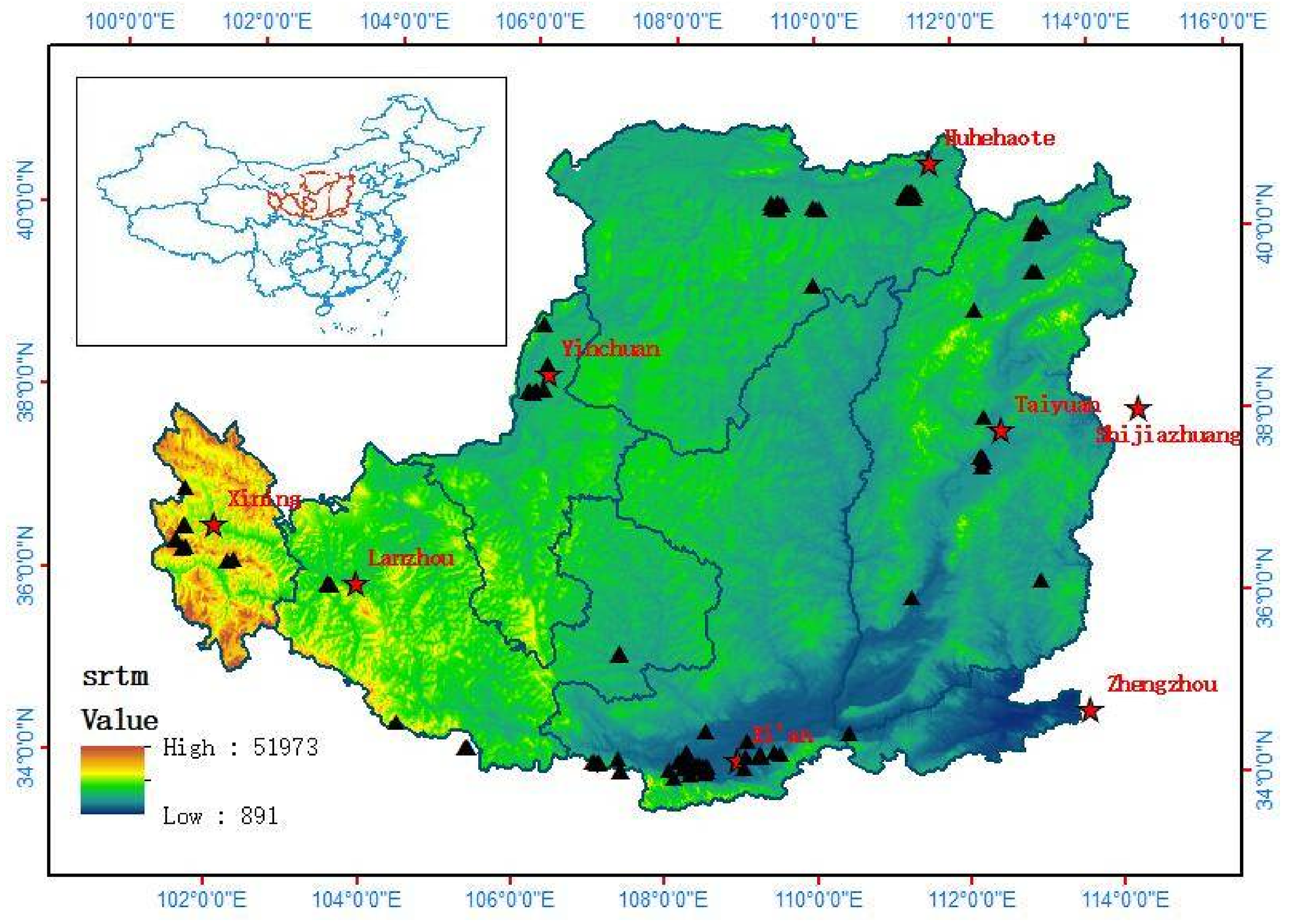
To verify the performances of the different GRACE solutions, the monthly groundwater level data from 136 monitoring wells across the Loess Plateau obtained from January 2005 to December 2014 were considered. The data were acquired from the China Geological Environment Monitoring Groundwater Table Yearbook that was published by the China Earth Publishing House. The distribution of these monitoring wells is shown in Figure 1. Some of these wells have incomplete data records, and the smaller data gaps for the wells were filled using a linear interpolation. Before comparing with the GWS changes estimated from the GRACE solutions, the well water-levels must be converted into GWS changes. The conversion method is given in Section 3.2.4.

3.1.4. Coal Mining Data

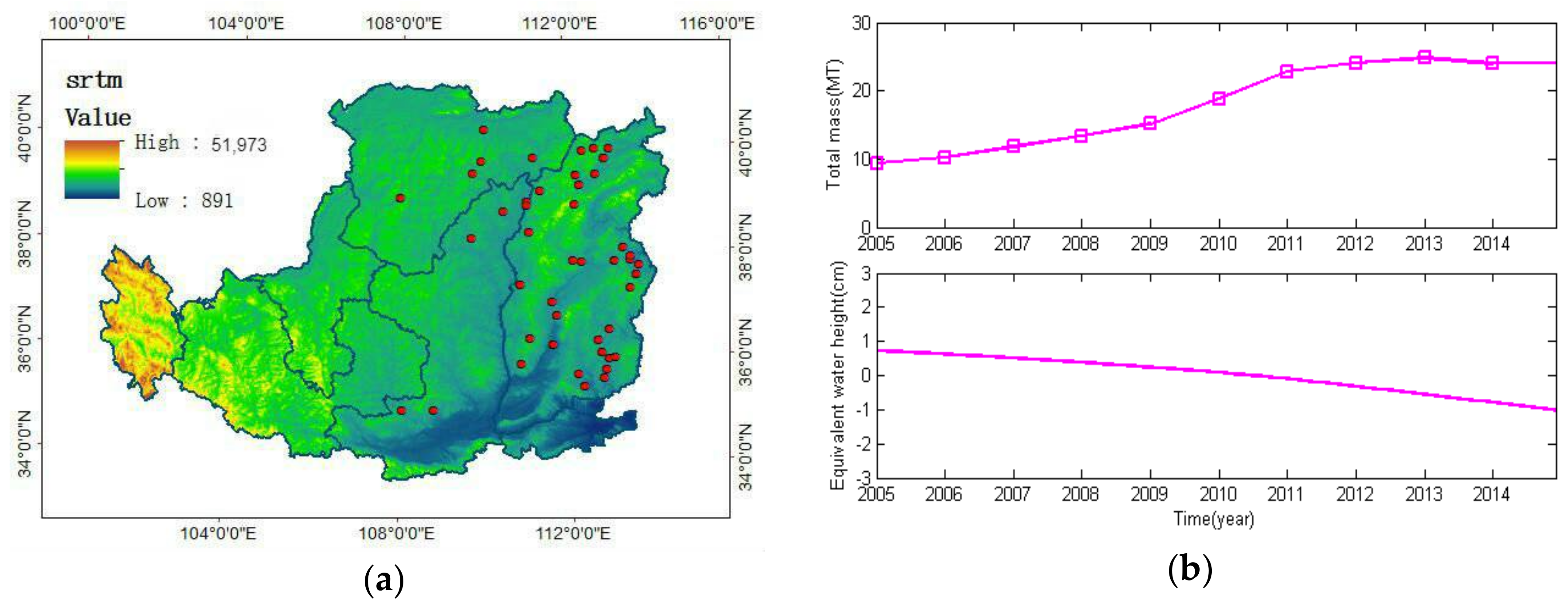
The Loess Plateau is an important energy base in China and provides large quantities of coal each year. Shanxi Province and Inner Mongolia Province in particular produce large quantities of coal, leading to an annual regional output of two billion tons. We have obtained the spatial distribution of locations with an annual output of more than 10 million tons over the Loess Plateau from the China Coal Industry Association, as shown in Figure 2a. We can see that most of the production occurs in and around Shanxi Province, with a few exceptions. Inevitably, the mass changes caused by coal mining are mistakenly identified as a part of the TWS changes estimated from the GRACE solutions. Therefore, coal mining must be deducted from the TWS before we calculate the GWS changes. In our research, we acquired the total annual amounts of coal mined across the Loess Plateau from 2005 to 2014 from the China Statistical Yearbook. For ease of comparison, we converted the mass changes from coal mining into changes of equivalent water heights, as shown in Figure 2b, and the conversion method is given in Section 3.2.6.

3.2. Methods

3.2.1. Calculating the TWS Changes from SH Solutions

The method proposed by Wahr et al. (1998) is used to convert the SH solutions into TWS changes in this study [24]. The specific formula is written as follows:

$$\Delta \mathrm{h}\left(\theta ,\mathsf{\lambda }\right)=\frac{\gamma {\rho }_{ave}}{{\rho }_{wat}}{\displaystyle \sum }_{l=0}^{\infty }{\displaystyle \sum }_{m=0}^l{\overline{P}}_{lm}\left(\cos \theta \right)\frac{2l+1}{1+k_l}\times \left(\Delta C_{lm}\cos \left(m\lambda \right)+\Delta S_{lm}\sin \left(m\lambda \right)\right)$$

(1)

In the formula given above, $\Delta \mathrm{h}$ is the TWS changes expressed in equivalent water heights; $\theta$ and $\lambda$ are respectively the co-latitude and longitude; $\gamma$ is the average radius of the Earth; ${\rho }_{ave}$ and ${\rho }_{wat}$ are respectively the average density of the Earth and the density of water; ${\overline{P}}_{lm}$ is the $l$th degree and $m$th order fully normalized Legendre function; $k_l$ is the elastic load Love number; and $\Delta C_{lm}$ and $\Delta S_{lm}$ are the changes in the Stokes coefficients from the GRACE solutions relative to a 2005–2014 mean baseline.

To reduce “stripe” noise and high frequency noise in the SH solutions, the decorrelation and Gaussian filters are usually necessary. Therefore, the new formula for calculating the TWS Changes from SH Solutions is written as follows [11,24]:

$$\Delta \mathrm{h}\left(\theta ,\mathsf{\lambda }\right)=\frac{\gamma {\rho }_{ave}}{{\rho }_{wat}}{\displaystyle \sum }_{l=0}^{\infty }{\displaystyle \sum }_{m=0}^l{\overline{P}}_{lm}\left(\cos \theta \right)W_l\frac{2l+1}{1+k_l}\times \left(\Delta {\widehat{C}}_{\mathrm{lm}}\cos \left(m\mathsf{\lambda }\right)+\Delta {\widehat{S}}_{lm}\sin \left(m\mathsf{\lambda }\right)\right)$$

(2)

$$\{\begin{array}{c}{W}_0=1/2\pi \\ W_1=1/2\pi \left(\left(1+exp\left(-2b\right)\right)/\left(1-exp\left(-2b\right)\right)-1/b\right)\\ \begin{array}{c}{W}_{l+1}=-\left(2l+1\right)W_l/b+W_{l-1}\\ \mathrm{b}=ln2/\left(1-cos\left(R/\gamma \right)\right)\end{array}\end{array}$$

(3)

where $W_l$ is the Gauss filter weight function, and it could be expressed as Equation (3), $R$ is the Gauss filter smooth radius, $\Delta {\widehat{C}}_{lm}$ and $\Delta {\widehat{S}}_{lm}$ are the residuals after deducting the correlated errors from $\Delta C_{lm}$ and $\Delta S_{lm}$. The detail steps for $\Delta {\widehat{C}}_{lm}$ calculation are as follows (take “P3M6” decorrelation filter for example) [32]: First, for the coefficients with order less than 6 $\left(\mathrm{m}<6\right)$, they remain unchanged; second, for the coefficients with order greater than or equal to 6 $\left(\mathrm{m}\ge 6\right)$, the correlated error is calculated with a cubic polynomial: $\Delta C_m\left(l\right)=a_0+a_{1}l+a_2{l}^2+a_3{l}^3$, where the polynomial coefficients are obtained by least-squares fit from $\Delta C_{l-4,m}$, $\Delta C_{l-2,m}$, $\Delta C_{l,m}$, $\Delta C_{l+2,m}$, $\Delta C_{l+4,m}$; Finally, after deducting the correlated errors from $\Delta C_{lm}$, we get $\Delta {\widehat{C}}_{lm}$: $\Delta {\widehat{C}}_{lm}=\Delta C_{lm}-\Delta C_m\left(l\right)$. $\Delta {\widehat{S}}_{lm}$ can be acquired in the same way.

3.2.2. Conversion from SH Solutions to Slepian Solutions

Supposing that the spherical harmonic basis functions represented by $Y_{lm}\left(\theta ,\lambda \right)$ are orthogonal over the entire sphere, the mathematical expression of the Slepian basis functions for a certain local region R on the sphere is written as follows [36,42,43,44]:

$$\{\begin{array}{c}{g}_a\left(\theta ,\lambda \right)={\displaystyle \sum _{l=0}^L}{\displaystyle \sum _{m=-l}^l}{g}_{a,lm}{Y}_{lm}\left(\theta ,\lambda \right)\\ g_{a,lm}={{\displaystyle \int }}_{\mathsf{\Omega }}{g}_a\left(\theta ,\lambda \right)Y_{lm}\left(\theta ,\lambda \right)d\mathsf{\Omega }\end{array}$$

(4)

In the formula given above, $g_a\left(\theta ,\lambda \right)$ are the Slepian basis functions, $g_{a,lm}$ are the parameters for converting the spherical harmonic basis functions into Slepian basis functions, $\theta$ and $\lambda$ are the co-latitude and longitude respectively, $L$ is the maximum order. The expressions of the global TWS changes, expressed with SH and Slepian functions, are as follows [42,44]:

$$\Delta \mathrm{T}\left(\theta ,\lambda \right)={\displaystyle \sum }_{l=0}^L{\displaystyle \sum }_{m=-l}^l\Delta {\mu }_{lm}{Y}_{lm}\left(\theta ,\lambda \right)={\displaystyle \sum }_{\alpha =1}^{{\left(L+1\right)}^2}\Delta v_{\alpha }{g}_a\left(\theta ,\lambda \right)\approx {\displaystyle \sum }_{\alpha =1}^N\Delta v_{\alpha }{g}_a\left(\theta ,\lambda \right)$$

(5)

$$v_{\alpha }={\displaystyle \sum }_{l=0}^L{\displaystyle \sum }_{m=-l}^l{\mu }_{lm}{g}_{\alpha ,lm}$$

(6)

$${\mu }_{lm}={\displaystyle \sum }_{\alpha =1}^{{\left(L+1\right)}^2}{v}_{\alpha }{g}_{\alpha ,lm}$$

(7)

$$\mathrm{N}={\left(L+1\right)}^2\frac{A}{4\pi }$$

(8)

In the formula above, $\Delta \mathrm{T}\left(\theta ,\lambda \right)$ is the TWS changes, $v_{\alpha }$ is the Slepian coefficient, ${\mu }_{lm}$ is the corresponding spherical harmonic coefficient, $\Delta {\mu }_{lm}$ is the spherical harmonic coefficient changes relative to a 2005–2014 mean baseline, and $\Delta v_{\alpha }$ is the Slepian coefficient changes relative to a 2005–2014 mean baseline, N is the Shannon coefficient, A is the area of the region R.

3.2.3. Calculating the Scale Factor for Restoring Signal Attenuation

The scale factor ($k$) can be calculated by the following formula [45]:

$$\mathrm{M}={{\displaystyle \sum }}^{\text{}}{\left(\Delta S_T-k\Delta S_F\right)}^2$$

(9)

where $\Delta S_T$ is the true (unfiltered) time series of the hydrological model or other model we used for signal recovery, which usually correlates well with the GRACE data; $\Delta S_F$ is the filtered time series of the model (filtered with the same filter applied to GRACE solutions). By minimizing the misfit between $\Delta S_T$ and $\Delta S_F$ through a simple least square regression, we can obtain the scale factor ($k$).

3.2.4. Calculating In Situ Groundwater from Monitoring Wells

For a single monitoring well, we can derive the GWS changes by multiplying the well water-level data by the basin-averaged specific yield. The GWS changes for the whole area can be calculated by the following formula [11,46]:

$$\Delta \mathrm{GWS}={\displaystyle \sum }_j^N{S}_j{C}_j\Delta h_j/{\displaystyle \sum }_j^N{C}_j$$

(10)

where $N$ is the number of subareas divided by the provincial boundaries in the study region, $C_j$ is the areas of these subareas, $\Delta h_j$ is the averages of the water-level variations of all monitoring wells in each subarea, and $S_j$ is the basin-averaged specific yields. The use of different specific yields to estimate the in situ GWS changes from the monitoring wells affects only the annual amplitudes at regional scales. Thus, we use 0.03 as the basin-averaged specific yield for all subareas to calculate the GWS changes.

3.2.5. Estimation of GWS Changes from GRACE

Since the mass loss caused by coal mining can reach the level of billions of tons per year in the Loess Plateau, the TWS changes estimated from GRACE in our work include not only the changes of GWS and surface water, but also the changes caused by coal mining. The GWS changes from GRACE can be estimated from the following formula:

$$\Delta \mathrm{GWS}=\Delta \mathrm{TWS}-\left(\Delta SM+\Delta SWE+\Delta C\right)$$

(11)

where $\Delta \mathrm{GWS}$ is the GWS changes, $\Delta \mathrm{TWS}$ is the TWS changes from GRACE, $\Delta SM$ and $\Delta SWE$ are changes of soil moisture and accumulated snow respectively (they can be acquired from GLDAS), and $\Delta C$ is the changes caused by coal mining.

3.2.6. Estimation of Groundwater Loss Caused by Coal Mining

Groundwater consumption caused by coal mining can be estimated by the following formulas [47,48]:

$${\mathrm{M}}_w={\mathsf{\mu }\mathrm{M}}_c$$

(12)

$$\Delta {\mathrm{h}}_c=\frac{{\mathrm{M}}_w}{A{\rho }_{wat}}$$

(13)

where ${\mathrm{M}}_c$ is the mass changes caused by coal mining, ${\mathrm{M}}_w$ is mass changes of the groundwater loss caused by mine drainage, $\mathsf{\mu }$ is the tons of coal drainage coefficient which represents the loss of groundwater for per ton of coal mined and 0.87 is used as the tons of coal drainage coefficient in this work [47,48]. ${\mathrm{M}}_w$ can be converted into equivalent water height ($\Delta {\mathrm{h}}_c$) using Equation (13), where ${\rho }_{wat}$ is the density of water, $A$ is the area of the research region.

4. Results

4.1. Scale Factor Estimation of SH Solutions and Mascon Solutions

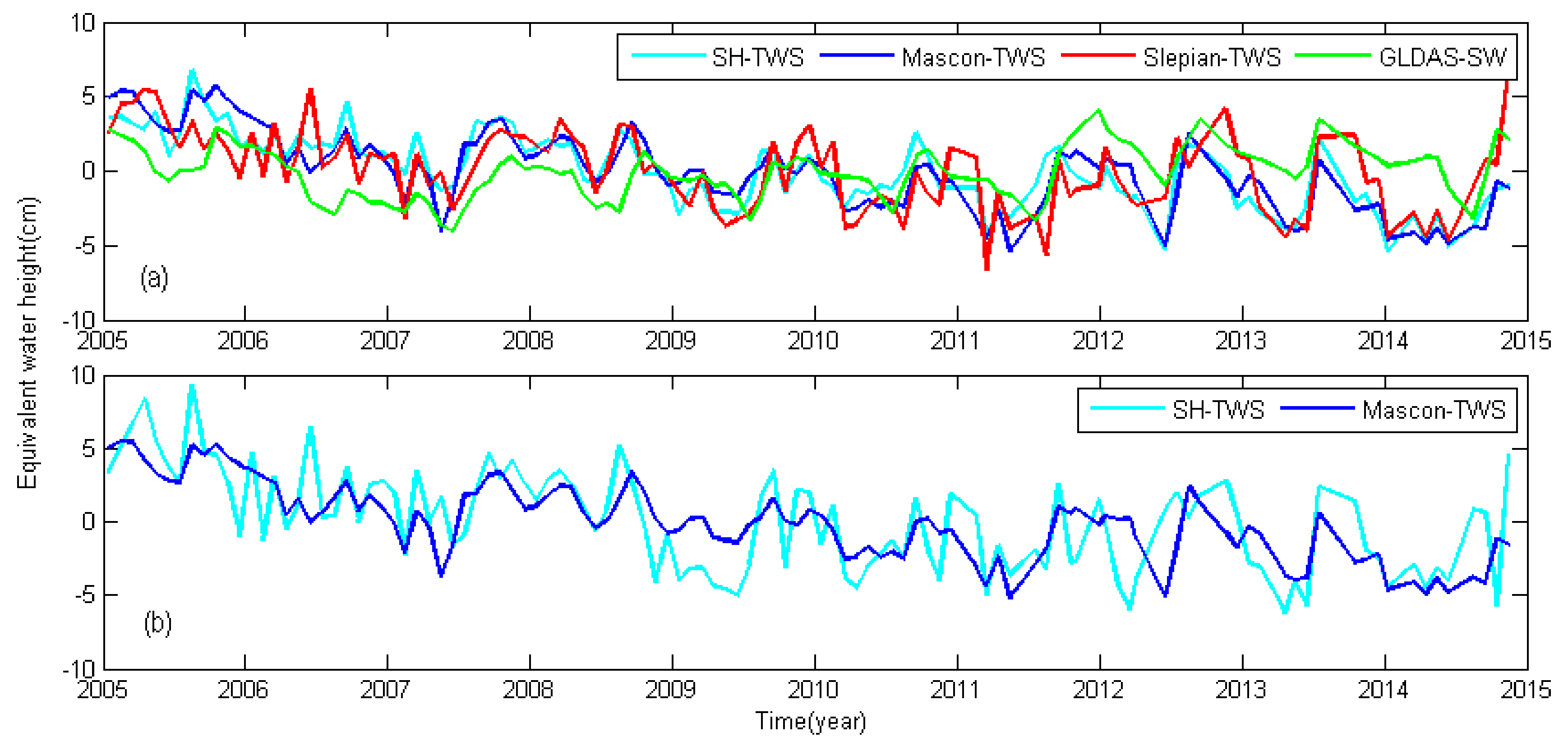
In most studies, Hydrological models have been used to calculate the scale factors for the signal recovery of SH solutions or mascon solutions; these calculations are based on the surface water changes of the Hydrological models which have high correlations with the TWS changes of the GRACE solutions. For the Loess Plateau, a series of factors, including its arid climate, intensive farm irrigation, and large amount of coal mining, result in poor correlations between the surface water changes from the Hydrological models and the TWS changes of the GRACE solutions. The correlation coefficient between the surface water changes from GLDAS (GLDAS-SW) and TWS from the SH solutions (SH-TWS) is 0.16, and the correlation coefficient between the GLDAS-SW and TWS from the mascon solutions (Mascon-TWS) is 0.33. Therefore, using Hydrological models is not advised when calculating the scale factors for this study area. The time series of the GLDAS-SW, Slepian-TWS, SH-TWS, and Mascon-TWS are shown in Figure 3a.

For the Slepian solutions, no decorrelation filtering or smoothing is required, resulting in fewer leakage errors and no losses of spatial resolutions. Moreover, the TWS from the Slepian solutions (Slepian-TWS) have high correlations with the SH-TWS or Mascon-TWS, with correlation coefficients of 0.78 and 0.77, respectively. Therefore, we estimated the scale factors for the signal recovery of the SH solutions and of the mascon solutions based on the Slepian solutions given in this research. A detailed description of the method for scale factors calculation is given in Section 3.2.3. Figure 3b shows the time series of the SH-TWS and Mascon-TWS after signal recovery. The amplitudes, phases and trends of the two time series, before and after signal restoration, are shown in

Table 1. Changes of two TWS (SH-TWS and Mascon-TWS) before and after signal restoration in term of amplitude, phase and trend, and the scale factors were used.

Time Series	Before Signal Restoration			After Signal Restoration			Scale Factor
	Amplitude (cm)	Phase (°)	Trend (cm/year)	Amplitude (cm)	Phase (°)	Trend (cm/year)
SH-TWS	1.32 ± 0.36	271 ± 15	−0.62 ± 0.09	1.85 ± 0.79	364 ± 24	−0.84 ± 0.20	1.35
Mascon-TWS	1.36 ± 0.40	302 ± 17	−0.67 ± 0.10	1.22 ± 0.39	302 ± 18	−0.69 ± 0.09	0.98

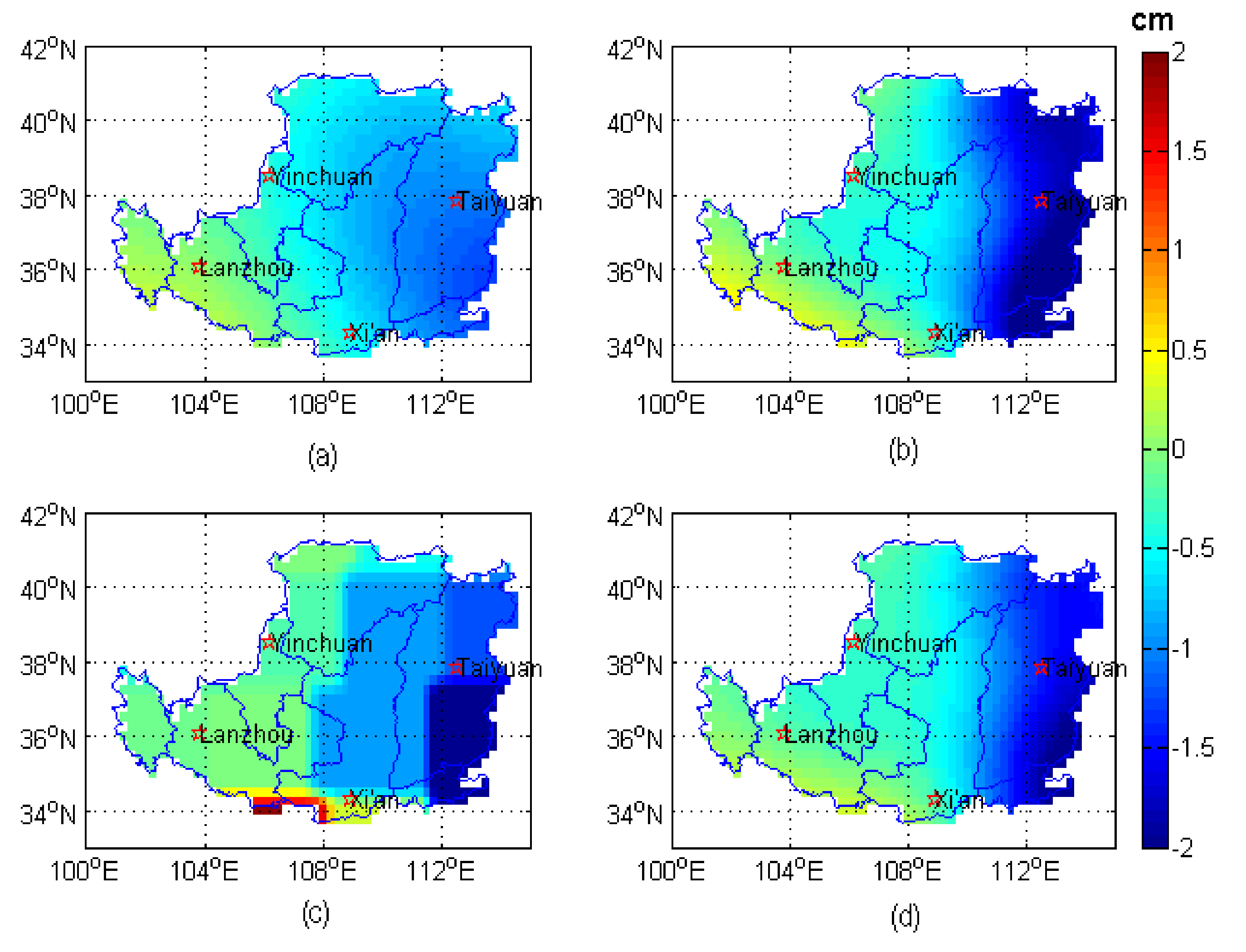
. This table shows the smaller influence of the scale factors on the Mascon-TWS, which may be due to the better signal-to-noise ratio of the mascon solutions. Figure 4 shows the spatial distribution of the changing trends of SH-TWS and Mascon-TWS before and after signal recovery, which show significant changes in both the SH-TWS and Mascon-TWS. After signal restoration, the trend is more concentrated, and the larger parts are distributed over the eastern part of the Loess Plateau, especially over Shanxi Province.

4.2. Comparison of Three GWS from GRACE Solutions and In Situ GWS

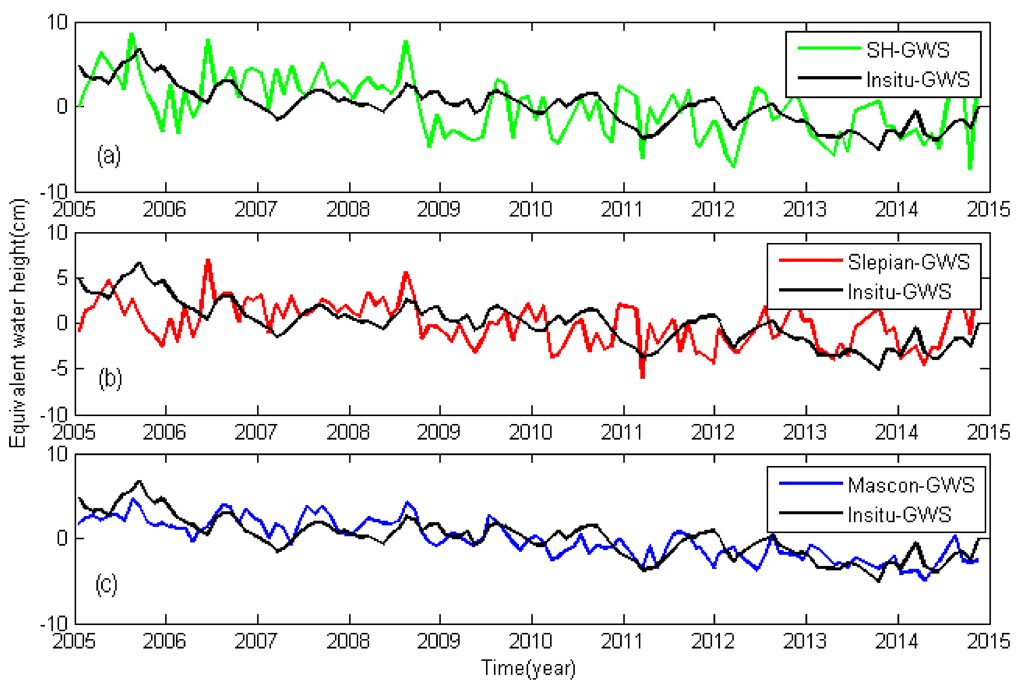
By subtracting the changes of the surface water and the changes caused by coal mining from the TWS changes estimated from the three types of GRACE solutions, we obtained three GWS change time series from 2005 to 2014 for the Loess Plateau. The changes of the surface water used here include the changes of the soil moisture and the changes of the accumulated snow, which were acquired from GLDAS. We calculated the in situ GWS changes from the monitoring wells according to Equation (10). The comparisons between GWS changes from the GRACE solutions and the in situ GWS changes derived from monitoring wells are shown in Figure 5.

In this study, we calculated the annual trends of the four GWS changes based on the least squares linear regression model, as shown in

Table 2. Comparisons of GWS anomalies of ground-based (In-situ GWS) and GRACE-based (SH-GWS, Slepian-GWS and Mascon-GWS) in terms of RMSE, correlation ($\mathsf{\rho }\prime$) and annual trend.

Variables	Annual Trend (cm/year)	$\mathsf{\rho }\prime$	RMSE (cm)
SH-GWS	−0.80 ± 0.18	0.46	3.11
Slepian-GWS	−0.37 ± 0.14	0.33	2.76
Mascon-GWS	−0.65 ± 0.07	0.72	1.66
In-situ GWS	−0.66 ± 0.08	1	-

. The annual trend of the GWS changes from the SH solutions (SH-GWS), the GWS changes from the mascon solutions (Mascon-GWS), and the GWS changes from the Slepian solutions (Slepian-GWS) are respectively $-0.80\pm 0.18$ cm/year, $-0.65\pm 0.07$ cm/year, and $-0.37\pm 0.14$ cm/year. Comparing the annual trend of the in situ GWS changes ($-0.66\pm 0.08$ cm/year) with the annual trends of the GWS changes from the GRACE solutions, we found that Mascon-GWS match the in situ GWS changes best. Additionally, the correlation coefficients and root mean square error (RMSE) values of the GWS changes from the GRACE solutions and the in situ GWS changes were calculated (Table 2). We found that Mascon-GWS performed better than SH-GWS and Slepian-GWS, showing the highest correlation coefficient and lowest RMSE values. The correlation coefficient of the Mascon-GWS with the in situ GWS changes is 0.72, while the correlation coefficients between SH-GWS and Slepian-GWS and the in situ GWS changes are respectively 0.46 and 0.33. The RMSE value of Mascon-GWS and the in situ GWS changes is 1.66 cm, while the RMSE values of SH-GWS and Slepian-GWS and the in situ GWS changes are 3.11 cm and 2.76 cm.

In summary, through the comparison and analysis of the GWS changes from the GRACE solutions and the in situ GWS changes derived from the monitoring wells, we find that the mascon solutions perform the best for the GWS estimations over the Loess Plateau. Therefore, in the following sections, the Mascon-GWS changes are used for the spatial-temporal analysis of GWS changes over the Loess Plateau during 2005–2014.

4.3. Spatiotemporal Analysis of GWS Changes in the Loess Plateau

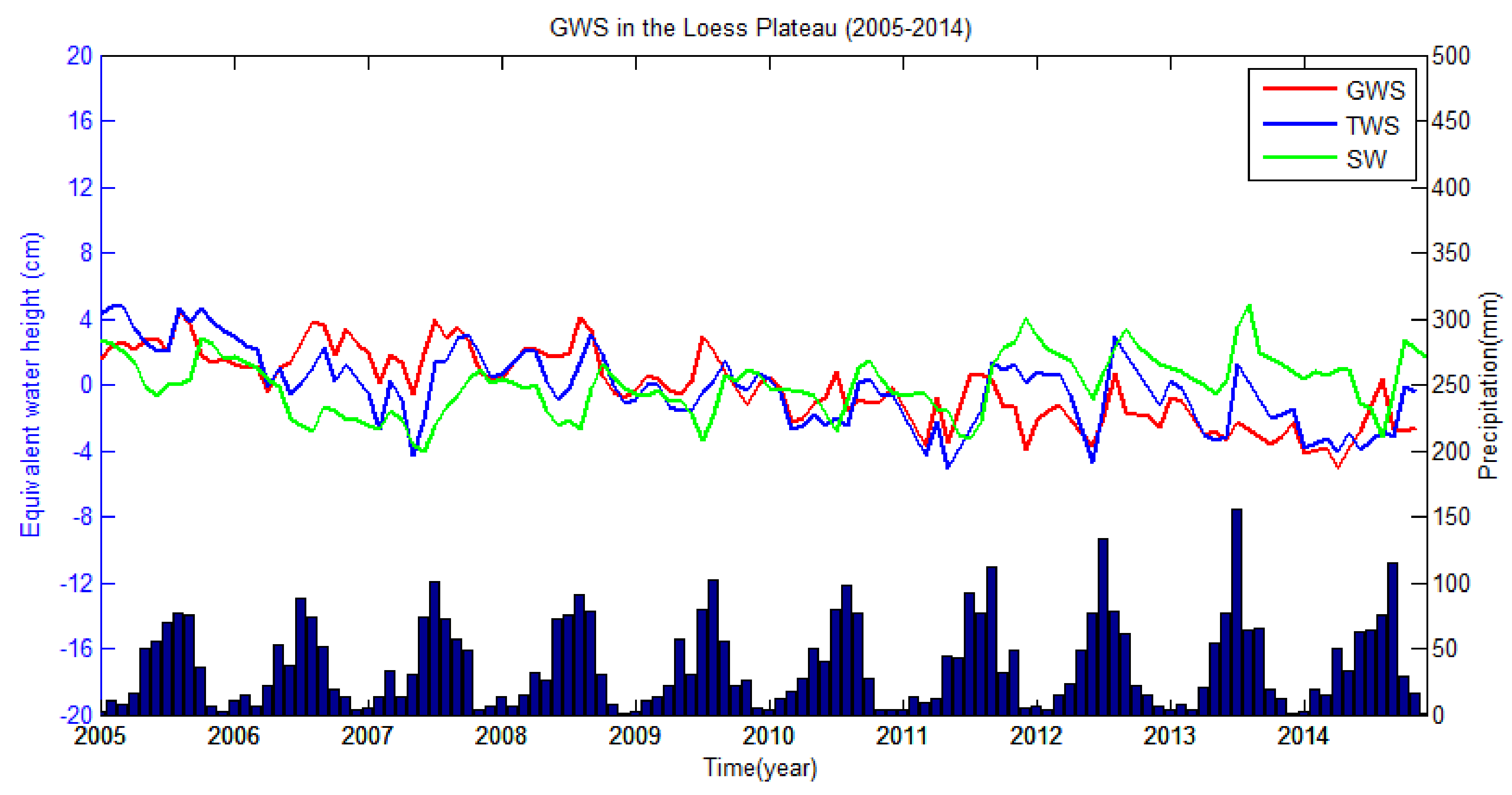
Figure 6 shows the monthly time series of the TWS changes (blue), surface water changes (green), GWS changes (red), and the precipitation data over the Loess Plateau from 2005 to 2014. We find that the rainfall over the Loess Plateau shows a strong seasonality, with more rainfall occurring in summer and autumn, accounting for more than 70% of the annual rainfall, while less rainfall occurs in winter and spring, accounting for only 20–30% of the total. Correspondingly, TWS changes, surface water changes, and GWS changes also show strong seasonality, with increases in summer and autumn and decreases in the spring and winter. This pattern indicates that rainfall plays an important role in the seasonal changes of the GWS and is an important source of groundwater recharge.

However, we also find that the TWS changes, surface water changes, GWS changes and precipitation do not agree well. First, the annual variation trends of the four time series for 2005–2014 differ, with surface water changes and precipitation showing increasing trends respectively of $0.13\pm 0.09$ cm/year and $0.12\pm 0.1$ cm/year, while the TWS changes and GWS changes show decreasing trends respectively of $-0.69\pm 0.09$ cm/year and $-0.65\pm 0.07$ cm/year. Second, the average annual rainfall increased via two jumps in 2007 and 2011, both showing increases of more than 50 mm, as shown in

Table 3. Precipitation during 2005 to 2014.

Variables	2005	2006	2007	2008	2009	2010	2011	2012	2013	2014
Precipitation 1	407	396	457	447	423	441	491	489	484	480

¹ The unit of precipitation is millimeter (mm).

. The TWS and surface water changes both show obvious increases in 2007 and 2011. However, the GWS changes show no obvious increases. Finally, the annual variation trends of the TWS changes, surface water changes and GWS changes are $-2.64\pm 0.49$ cm/year, $-2.13\pm 0.64$ cm/year and $-0.40\pm 0.32$ cm/year from 2005 to 2006 and are $-0.55\pm 0.13$ cm/year, $0.34\pm 0.11$ cm/year and $-0.71\pm 0.10$ cm/year from 2007 to 2014, as shown in

Table 4. Trends of TWS, surface water and GWS.

Variables	2005 January–2006 December	2007 January–2014 December	2005January–2014 December
TWS-TREND 1	−2.64 ± 0.49	−0.55 ± 0.13	−0.69 ± 0.09
SW-TREND 1	−2.13 ± 0.64	0.34 ± 0.11	0.13 ± 0.09
GWS-TREND 1	−0.40 ± 0.32	−0.71 ± 0.10	−0.65 ± 0.07

¹ The unit of trend is centimeter per year (cm/year).

. These values indicate that the surface water changes have opposite trends during the two time periods, and the TWS changes show a more serious decline in the first time period, while the GWS changes show a more serious decline in the second time period. Therefore, we can conclude that rainfall greatly influences the surface water, but is not the main reason for groundwater consumption in the Loess Plateau; thus, human activities may play an important role in the groundwater consumption.

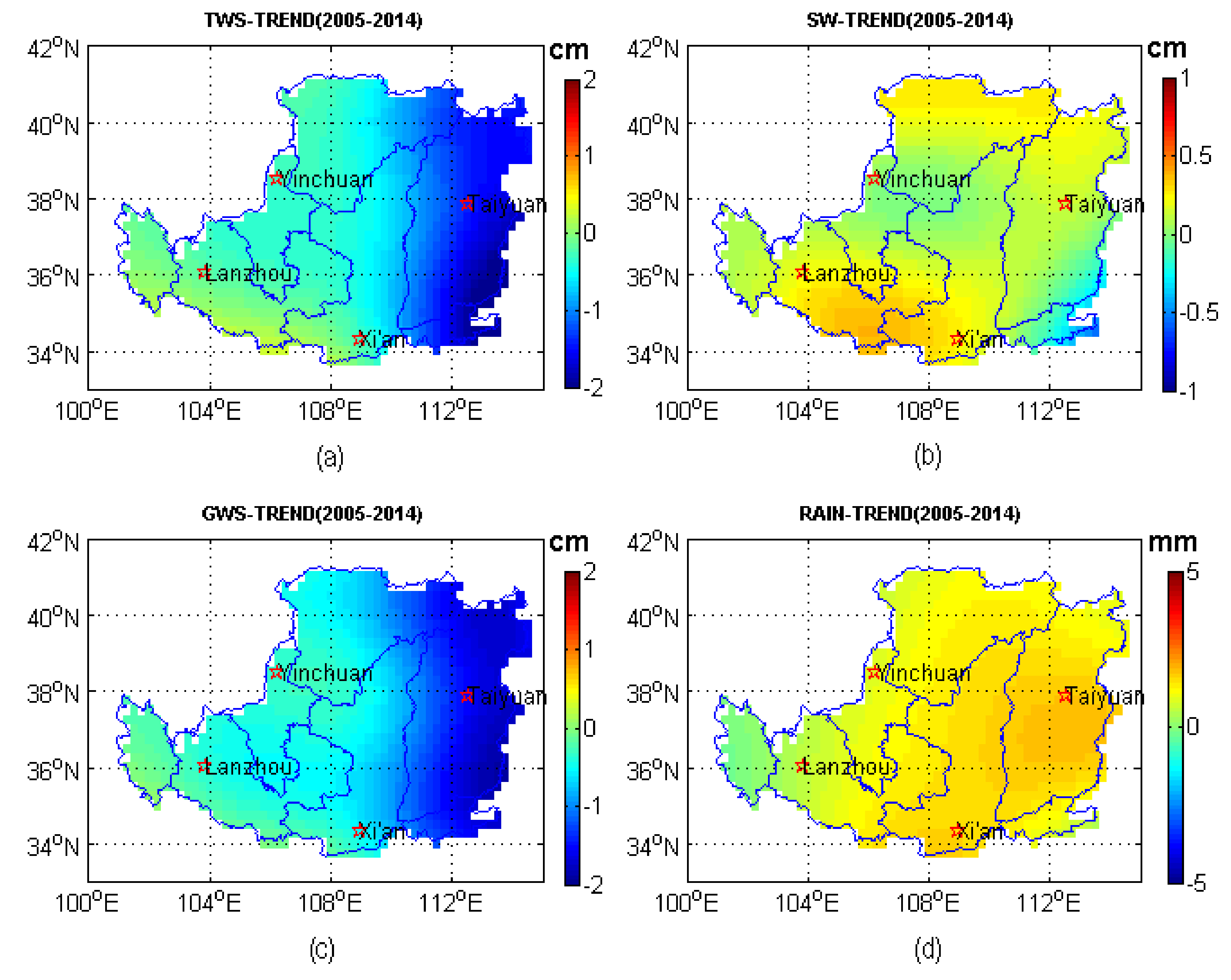
Figure 7 shows the spatial distributions of the annual variation trends of the TWS changes, surface water changes and GWS changes during 2005–2014. We find that the surface water and rainfall show increasing trends across the whole region for this decade, while the TWS and GWS show decreasing trends. The spatial distribution of the GWS trends is basically similar to the spatial distribution of the GWS trends, and both show stronger decreases in the eastern region, including in Shanxi Province and those parts of Inner Mongolia and Henan Province adjacent to Shanxi Province. The descending trends in the eastern region are several times greater than those in other regions, with the former are about −1.5 cm/year and the latter are about −0.5 cm/year. While establishing the relationship between the GWS and rainfall, we found that the GWS and the rainfall trend do not show any consistency in their spatial distributions, especially in the eastern region, where the rainfall showed an increasing trend, but the groundwater consumption was the most serious. Once again, this result proves that the main mechanism of groundwater consumption in the Loess Plateau is not rainfall. It is note that the impact of coal mining is not subtracted when analyzing the spatial distribution of TWS and GWS trends due to the inaccessibility of the coal mining data for each location across the Loess Plateau.

4.4. Influence of Coal Mining on GWS Changes

As shown in Figure 2, there is a large number of large-scale coal mines in the Loess Plateau that represent the important coal mining centers, especially those in Shanxi Province. The total annual output of these mines has reached approximately 2 billion tons since 2012. Large-scale coal mining operations may have two types of impact on the GWS estimates. On one hand, the qualitative changes caused by coal mining will directly affect the estimations of groundwater from GRACE data, although these changes have been deducted from the TWS changes in the above analysis (except spatial distributions of the annual variation trends). On the other hand, large-scale coal mining may destroy the aquifer, resulting in serious groundwater losses, which is mainly caused by mine drainage. And the loss of groundwater caused by coal mining can be estimated using the formulas given in Section 3.2.6. 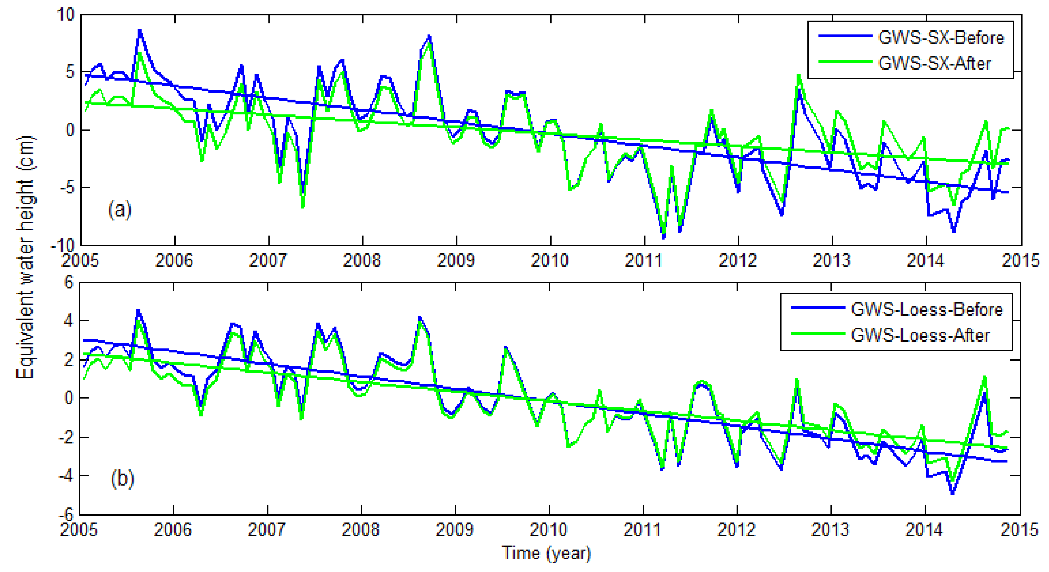Figure 8a shows the GWS changes in Shanxi Province before and after deducting the loss of groundwater caused by coal mining. We find that before deducting the groundwater loss due to coal mining, the groundwater consumption in Shanxi Province is more serious, reaching $-0.96\pm 0.11$ cm/year; after deducting this loss, the groundwater consumption rate of Shanxi Province ($-0.56\pm 0.16$ cm/year) is basically the same as the groundwater consumption rate in the other regions of the Loess Plateau (about −0.5 cm/year). The slight difference may be due to the inaccuracy of the coal mining data or the tons of coal drainage coefficient. The result may explain why there is a large difference in the rates of groundwater consumption, when there are only slight differences in the precipitation and surface water between the eastern region and the other regions in the Loess Plateau.

Figure 8b shows the time series of the groundwater before and after deducting the groundwater consumptions caused by the coal mining across the Loess Plateau, and the trends are respectively $-0.65\pm 0.07$ cm/year and $-0.49\pm 0.07$ cm/year. The latter groundwater consumption may be caused by the industrial, drinking and irrigation water use across the Loess Plateau. Since no specific amount of coal can be acquired for each location, the spatial distributions of GWS trends after deducting the groundwater consumption due to coal mining are not given in this paper. However, by comparing the spatial distribution of GWS and the map of the large-scale coal mines of the Loess Plateau (as shown in Figure 2a), the large coal mines are clearly found to be mainly concentrated in those areas with serious groundwater consumption. 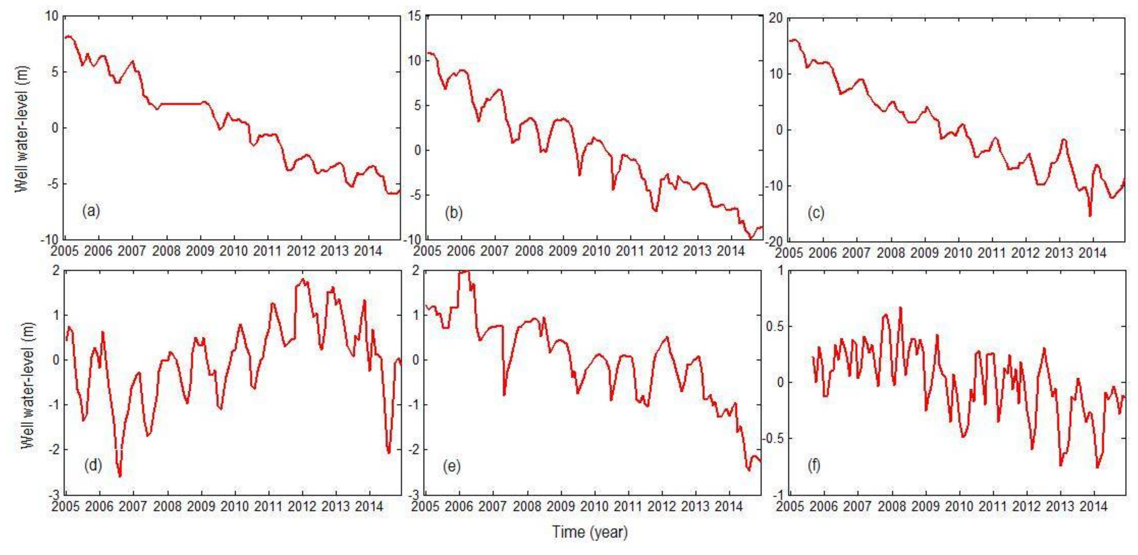Furthermore, Figure 9 shows water-level changes from some significant wells: Figure 9a–c show the water-level changes of wells from the areas more affected by coal mining and Figure 9d–f show the water-level changes of wells from the area far from mining area. It is obvious that water-level changes of wells from the areas more affected by coal mining show more serious decline. Therefore, we can conclude that the larger groundwater consumption in the eastern Loess Plateau is due to coal mining.

5. Discussion

In this study, three types of GRACE solutions, that is, the SH solutions, Slepian solutions and mascon solutions, were used to monitor the GWS changes of the Loess Plateau from 2005 to 2014. We find that the three TWS changes estimated from three GRACE solutions agree well and the performance for GWS estimation decrease in order of mascon solutions, SH solutions and slepian solutions. In a previous study, Ashraf et al. [23] compared and analyzed the performance of three GRACE solutions in the inversion of TWS in Africa. Correlation coefficients 0.62–0.89 were observed in medium-size regions of interest (ROIs) between Slepian-TWS and the SH-TWS or Mascon-TWS, which were generally consistent with our results. However, they reached the conclusion that slepian solutions and mason solutions behave better than SH solutions for TWS estimations in small and medium-sized areas, which is somewhat different from the results obtained in our research. In our view, there are several doubts about their conclusions. First, they point out that the filtering on the SH solutions will cause leakage errors and signal attenuation (reflected in changes of amplitude and phase), but the leakage errors and signal attenuation can be reduced by using the scale factor. Second, they believe that the leakage errors are few for the slepian solutions because no filter is used, but they did not analyze whether there are other uncertainties in the slepian solutions. Third, from the statistical data they provided, we find that the TWS trends from SH solutions match better with TWS trends from mascon solutions than that from slepian solutions, which is contrary to their conclusions. Finally, they did not validate their results with in situ wells data or any other observed data. Therefore, we think that the results obtained in our work are more reliable, and some unknown uncertainties when using the slepian method for GRACE data processing result in the slepian-GWS obtained in this study, being poorer than SH-GWS or Mascon-GWS. However, considering that Slepian solutions need no decorrelation filtering or smoothing, thus resulting in fewer leakage errors and no loss of spatial resolution. Slepian solutions can replace the hydrological model to calculate the scale factors of the SH solutions and the mascon solutions when the correlations between the surface waters from the hydrological models and the TWS from the GRACE are poor.

The final estimate of the groundwater depletion rate in the Loess Plateau from 2005–2014, based on the GWS changes estimated from the mascon solutions and the in situ GWS changes from the monitoring wells, were respectively $-0.65\pm 0.07$ cm/year and $-0.66\pm 0.08$ cm/year. Despite the fact that the difference between the groundwater depletion rates obtained from two GWS changes is small, some uncertainties still exist in the two GWS changes results. On the one hand, the monitoring wells in the Loess Plateau are few and unevenly distributed, so there may be some uncertainty in the estimation of in situ GWS changes. On other hand, with regards to the mass loss caused by coal mining, this paper has adopted the monthly average values calculated based on the total annual changes, which may be different from the real data. Therefore, a uniform spatial distribution of more monitoring well stations in the Loess Plateau is required as this will provide more reliable in situ GWS changes and further validate the estimated results from GRACE solutions. In addition, accurate monthly coal mining data should be obtained to accurately deduct the quality change caused by coal mining.

Based on the coal mining data, it was determined that the groundwater consumption rate in the Loess Plateau, after deducting the groundwater loess caused by coal mining, was approximately $-0.49\pm 0.07$ cm/year from 2005–2014, and that the serious groundwater consumption in the eastern Loess Plateau was caused by coal mining. This is only a relatively macroscopic result in terms of the groundwater consumption in the Loess Plateau. In future, it is possible to collect detailed coal mining data on the Loess Plateau to obtain the spatial distribution of groundwater losses caused by coal mining and groundwater consumption caused by industry, irrigation and drinking. In addition, once we have access to more accurate surface water changes and GWS changes, we can also estimate the mass loss caused by coal mining by subtracting the surface water changes and GWS changes from the TWS changes estimated from GRACE solutions. These can then be used to monitor monthly coal mining in various locations over the Loess Plateau.

6. Conclusions

This study uses GLDAS data, coal mining data and GRACE satellite gravity data to study the groundwater changes of the Loess Plateau from 2005 to 2014. Since the different GRACE solutions vary, we estimated the groundwater variations from three types of GRACE solutions, that is, the SH solutions, Slepian solutions and mascon solutions. By comparing the GWS changes results from different GRACE solutions with the in situ GWS changes calculated from 136 groundwater observation wells, we find that the GWS changes from mascon solutions match best with in situ GWS changes, because it shows the highest correlation coefficient, lowest root mean square error (RMSE) values and nearest annual trend, with in situ GWS changes. Therefore, we recommend the Mascon solutions for GWS change estimation in the Loess Plateau or other regions in the world. It is noted that the scale factors for the signal recovery of SH solutions or mascon solutions were calculated based on the Slepian solutions instead of hydrological models, due to the poor correlation between hydrological models and the GRACE data in the Loess Plateau. The results showed that the Slepian solutions perform well for the calculation of scale factors. This method can also be applied in other areas, especially in those that the correlations between hydrological models and GRACE data are poor.

Based on the GWS estimated from the mascon solutions, we analyzed the temporal and spatial variations of the groundwater in the Loess Plateau. First, we found that the GWS shows a strong seasonality, with increases in summer and autumn and decreases in spring and winter. Second, the groundwater of the Loess Plateau showed serious depletion during 2005–2014, and the annual variation trend was $-0.65\pm 0.07$ cm/year. Finally, the groundwater consumption of the eastern Loess Plateau (Shanxi Province and its surrounding areas) is more extreme, reaching $-0.96\pm 0.11$ cm/year. Furthermore, the precipitation data and coal mining data were used for analyzing the causes of the groundwater depletion, a comparison of the precipitation data, coal mining data and GWS change data showed that rainfall is the main reason for the seasonal variations of groundwater but is not the main reason for the persistent consumption of groundwater, and that groundwater losses due to the large-scale coal mining (mine drainage) was the main reason for the serious groundwater consumption in the eastern Loess Plateau from 2005 to 2014. After deducting the consumption of groundwater due to coal mining, the normal groundwater consumption for the Loess Plateau is −0.49 ± 0.07 cm/year.

Our research shows that the groundwater consumption in the Loess Plateau is severe, and in the eastern region, in addition to normal groundwater consumption, the consumption of groundwater caused by coal mining is huge. The results are helpful for the management and budget of groundwater resources, and can provide decision support for balancing the relationship between coal mining and groundwater resources protection, and maintaining the harmonious development of economy and nature. The analysis method used in this paper is also applicable to other mining areas, but it should be noted that the mining volume needs to reach a certain order of magnitude to ensure that the quality changes can be observed in the GRACE data.