Low-Rank and Sparse Matrix Decomposition with Cluster Weighting for Hyperspectral Anomaly Detection


Science and Technology on Automatic Target Recognition Laboratory, National University of Defense Technology, Changsha 410073, China
*
Author to whom correspondence should be addressed.
Remote Sens. 2018, 10(5), 707; https://0-doi-org.brum.beds.ac.uk/10.3390/rs10050707
Submission received: 17 March 2018
/
Revised: 1 May 2018
/
Accepted: 2 May 2018
/
Published: 4 May 2018
(This article belongs to the Section Remote Sensing Image Processing)
Abstract
:Hyperspectral anomaly detection plays an important role in the field of remote sensing. It provides a way to distinguish interested targets from the background without any prior knowledge. The majority of pixels in the hyperspectral dataset belong to the background, and they can be well represented by several endmembers, so the background has a low-rank property. Anomalous targets usually account for a tiny part of the dataset, and they are considered to have a sparse property. Recently, the low-rank and sparse matrix decomposition (LRaSMD) technique has drawn great attention as a method for solving anomaly detection problems. In this letter, a new anomaly detection method based on LRaSMD and cluster weighting is proposed. We concentrate on the sparse part, which contains most of anomaly information, and calculate the initial anomaly matrix based on this part. To suppress background regions and discriminate anomalies from the background more distinctly, a weighting strategy in terms of the clustering result is used, and then the anomaly matrix is updated. The judgement of anomalies is made according to the responses on the matrix. Our proposed method considers the characteristics of anomalies from the spectral dimension and the spatial distribution simultaneously. Experiments on three hyperspectral datasets demonstrate the outstanding performance of the proposed method.
1. Introduction
Hyperspectral imagery (HSI) is important in remote sensing applications, because it provides abundant spatial and spectral information for Earth observation. Target/anomaly detection is a significant research topic in hyperspectral remote sensing [1,2,3,4,5]. In a target detection task, the prior information of interested objects’ spectral signatures is necessary. So, it can be carried out when target signatures are known. In situations where target signatures are unavailable, we need to utilize anomaly detection algorithms to search for interested regions. In recent decades, anomaly detection has attracted much attention in the HSI processing field [6,7,8].
Anomalous targets in HSI consist of a few pixels or subpixels whose spectral signatures are extremely different from the homogenous background. In general, anomaly pixels occupy only a tiny part of the image, and the main task of an anomaly detector is to distinguish them from the background. There are plenty of anomaly detection algorithms that have been proposed in the past; the Reed-Xiaoli detector (RX) [9] is one of the most typical methods therein. It simply models the background as a multivariate Gaussian distribution and calculates the square root of the Mahalanobis distance between the pixel under test and the background. The RX detector is computationally efficient and has good detection performance on the datasets which satisfy the assumed background distribution model. Furthermore, a series of improved algorithms based on the RX detector have been proposed and widely used, such as the kernel RX (KRX) [10], the cluster kernel RX (CKRX) [11], the subspace RX (SSRX) [12], the weighted RX [13], the cluster-based anomaly detector (CBAD) [14], and the dual window-based eigen separation transform detector (DWEST) [15]. Apart from the aforementioned methods, some other concepts and techniques have also been introduced in anomaly detection. For instance, the blocked adaptive computationally efficient outlier nominator detector (BACON) [16] tries to purify the background model through robust statistics obtained from subsets of the dataset, which can improve the detection performance. The collaborative representation-based detector (CRD) [17] assumes that background pixels can be well represented by the linear combination of its spatial neighbors, while anomaly pixels cannot. In Reference [18], anomaly detection is conducted by adopting a Gaussian Mixture Model (GMM) to describe the statistics of the background, and the number of Gaussian components is automatically assessed by a mixture learning technique. In Reference [19], a metric is developed to account for anisotropic heavy tails in covariance-whitened data. It can be used to improve the detection results of other existing methods. Moreover, some low-rank-based anomaly detection methods have also been researched in depth. In Reference [20], the spectral unmixing algorithm is first applied to obtain the abundance vectors. Afterwards, a dictionary is built by using the mean-shift clustering of the abundance vectors. Finally, the low-rank decomposition based on the dictionary is proposed to extract anomaly objects. In Reference [21], a source component-based anomaly detection approach is designed, which uses the blind source component separation and identifies the components that are anomalous (or salient) compared to other components. It converts the anomaly detection to a low-rank matrix decomposition problem with the minimum volume constraint for the multi-modular background and sparsity constraint for the anomaly pixels. Recently, the low-rank and sparse matrix decomposition (LRaSMD)-based anomaly detection method [22] was proposed, which calculates the Euclidean distance between each pixel and the mean vector on the sparse part. Moreover, the LRaSMD-based Mahalanobis distance method (LSMAD) [23] utilizes the low-rank component and calculates the Mahalanobis distance for the test pixel. These LRaSMD-based methods all yield superior detection performance compared with other state-of-the-art detectors. However, they only consider the anomaly pixels’ spectral characteristics, but ignore their spatial distribution characteristics, which may influence the detection performance to some extent.
A novel anomaly detection method, which combines LRaSMD and cluster weighting, is proposed in this letter. For an original HSI dataset, the LRaSMD technique is first applied. Then we focus on the sparse matrix and calculate the -norm of each pixel on this component. The result can be denoted as the initial anomaly matrix. It is considered that some information about the background with a sparse property may be contained in the sparse part. Therefore, these background pixels have high responses on the initial anomaly matrix, which can weaken the detection performance. So, in this method, a cluster weighting strategy is designed. Based on the result of -means clustering, homogenous domains larger than the threshold are suppressed through a weighting function. Finally, an updated anomaly matrix with more reasonable anomaly values is obtained, which is deemed as the final detection result. The main advantages of our proposed method include: (1) making full use of the sparse property of anomalous targets to detect them from the perspective of spectral difference; (2) taking into account the spatial distribution characteristic of anomalous targets, which makes the detection result more accurate.
The remainder of the letter is organized as follows. Section 2 briefly introduces the LRaSMD model, and then describes our proposed method in detail. Section 3 gives the experimental results and parameter analysis. The discussion part is presented in Section 4. Finally, conclusions are drawn in Section 5.
2. LRaSMD with Cluster Weighting for Anomaly Detection
2.1. LRaSMD Model for HSI Dataset
Assume an HSI dataset can be represented by a matrix , where and denote the number of image pixels and spectral bands, respectively. It can be decomposed to a background matrix and an anomaly matrix , which is defined as:
However, in real-world situations, the observed data is always contaminated by noise, which can be modeled as independent and identically distributed Gaussian noise. Therefore, Equation (1) is modified as:
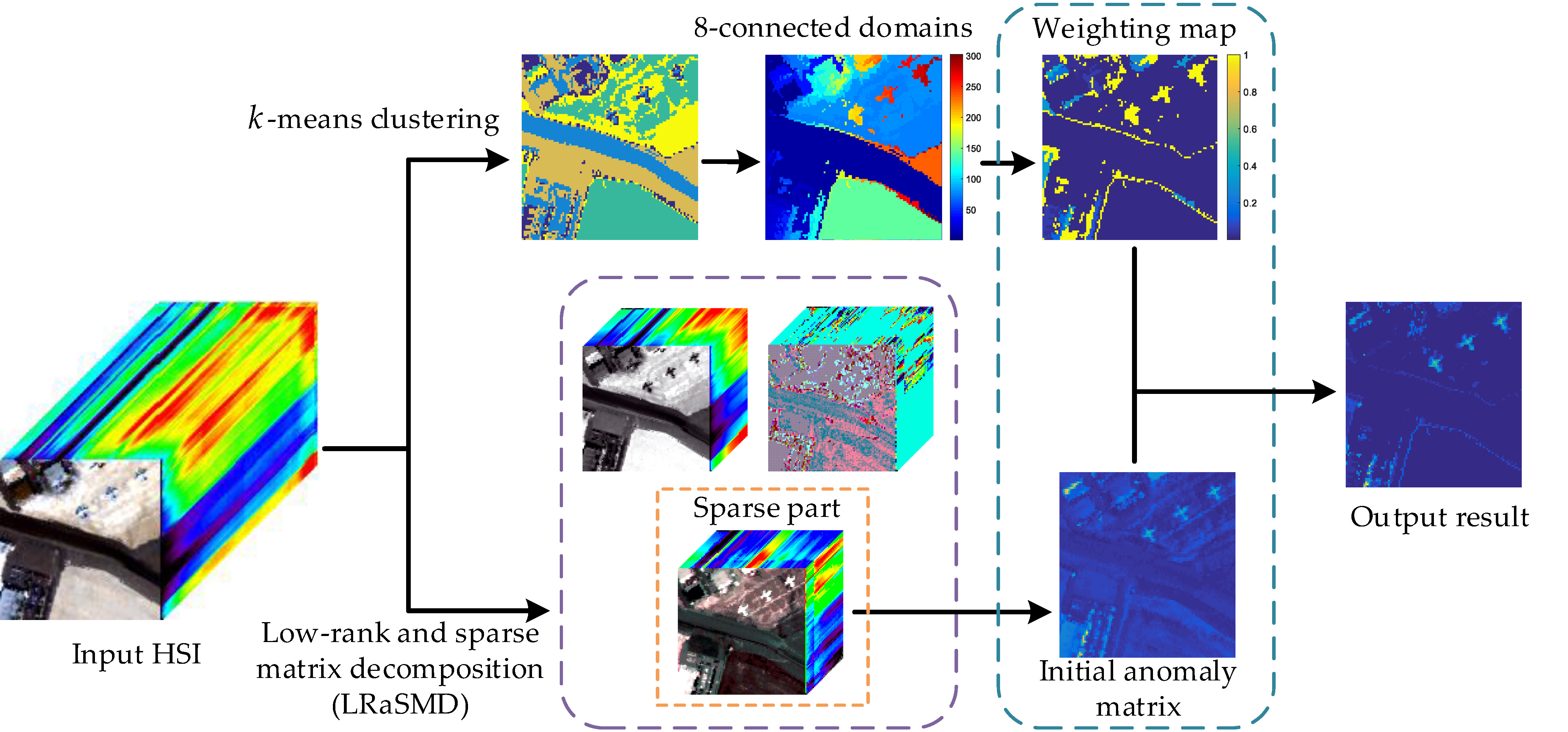
where is the noise matrix. For one specific HSI dataset, the background spectral signatures can be denoted as the linear combinations of several endmembers. So, matrix is considered to lie in a low-dimension subspace, which has a low-rank property. Moreover, anomalies in the dataset always have a low probability of occurrence. Thus, matrix can be assumed to have a sparse property. Therefore, the HSI dataset can be decomposed into Equation (2) by using the LRaSMD technique [22,23,24,25,26]. Figure 1 shows the decomposed data cubes of different parts.
In recent years, some fast and effective methods have been developed to solve the problem of LRaSMD, such as the randomized approximate matrix decomposition (RAMD) [27] and the robust principal component analysis (RPCA) [28]. In this letter, the Go Decomposition (GoDec) algorithm [29] is applied. It is a fast version for “low-rank + sparse” decomposition, which uses the bilateral random projections (BRP) to replace the singular-value decomposition (SVD) in the algorithm. The GoDec algorithm works through minimizing the decomposition error in Equation (2):
where is the Frobenius norm, and and represent the upper bound of the rank of and the cardinality (i.e., the sparsity level) of , respectively. The optimization problem in Equation (3) can be solved by alternatively solving two subproblems as follows:
where is the iteration time. In order to reduce the time cost, the BRP-based low-rank approximation is implemented to solve Equation (4). Then is updated as:
where and , wherein and are random matrices.
In each iteration, is updated through the entry-wise hard thresholding of as follows:
where represents the nonzero subset of the first largest entries of , and refers to a matrix’s projection to an entry set .
2.2. Anomaly Detection Based on LRaSMD and Cluster Weighting
According to the derivation aforementioned, an HSI dataset can be decomposed into one low-rank background matrix, one sparse anomaly matrix, and one noise matrix. The low-rank background matrix contains most of the background information, and the sparse anomaly matrix extracts the anomaly part effectively. Besides, the distribution of different components in the image also contains substantial spatial information. Based on this idea, some related works have already been conducted in the fields of HSI classification [30] and soil detection in multispectral images [31]. In this letter, we try to detect anomalies from HSI by taking advantage of the sparse matrix and considering the spatial distribution characteristics of the anomaly/background simultaneously. This approach is elaborated as follows.
For the tested HSI datase t , the GoDec [29] algorithm is executed, then three decomposed components in Equation (2) are obtained. Assume the sparse anomaly matrix can be denoted as , whose columns are spectral vectors. For each pixel, the initial anomaly value is calculated by using its -norm:
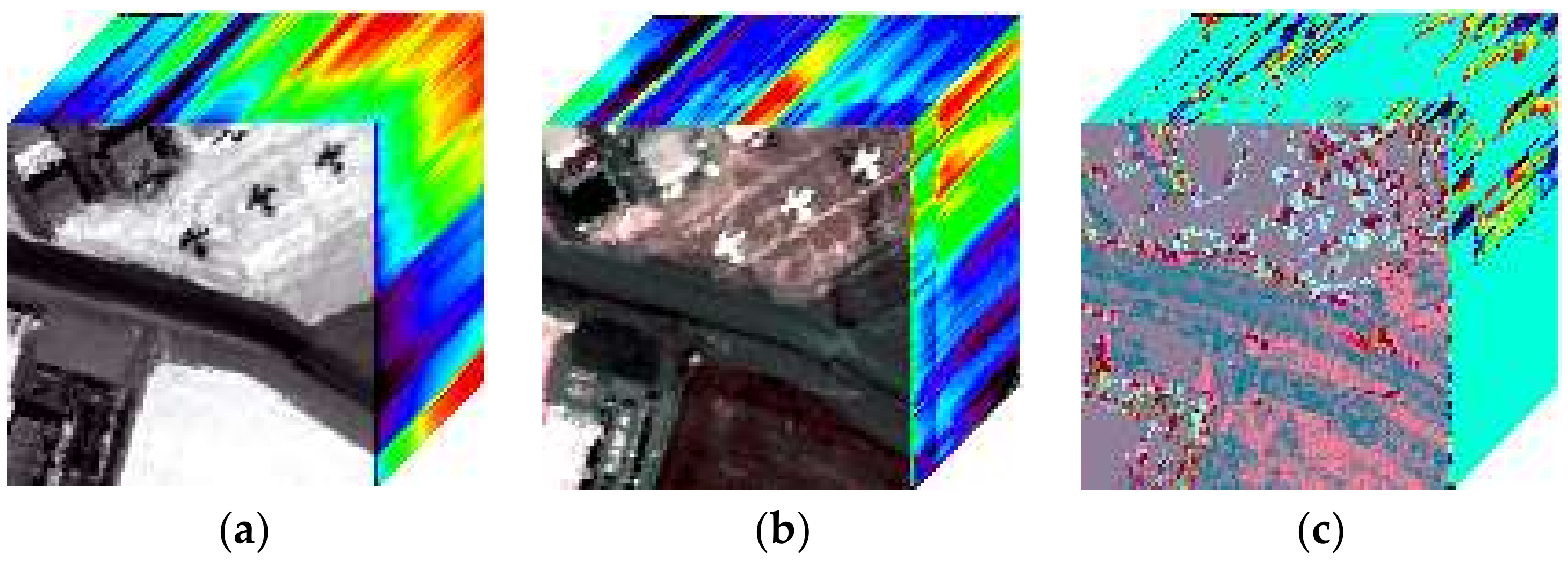
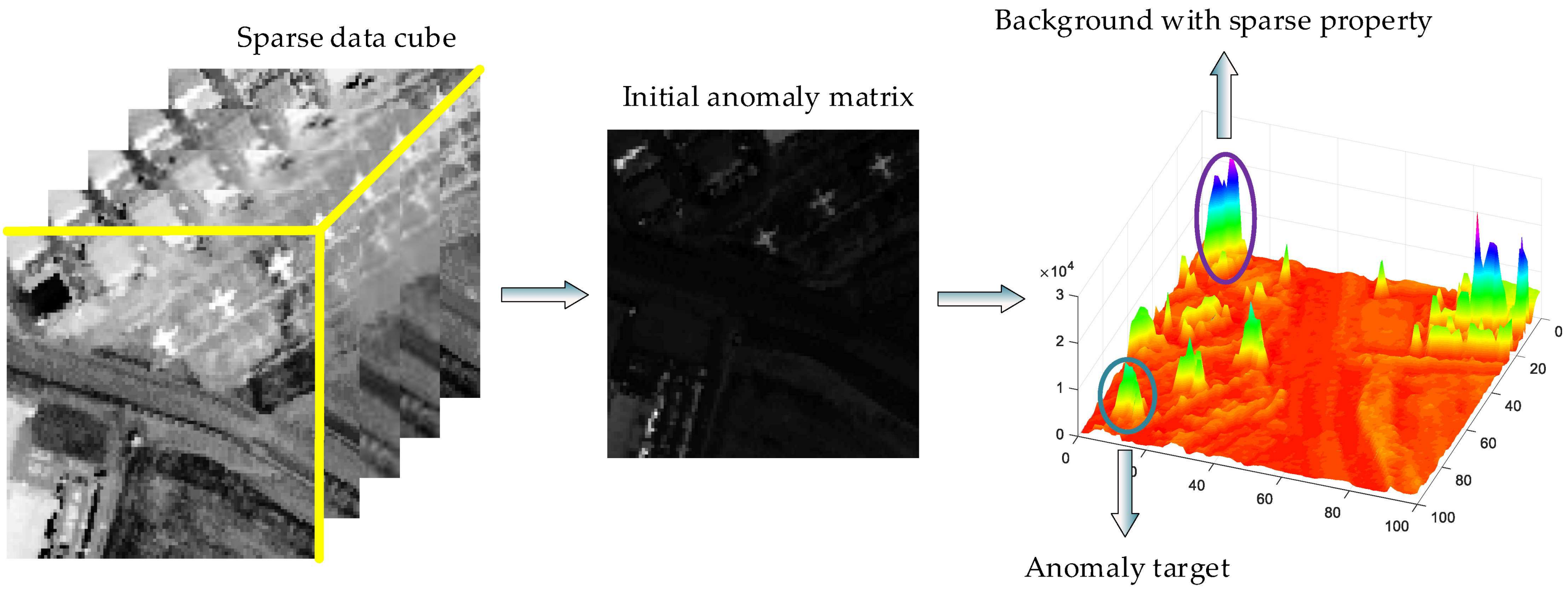
Equation (7) reflects the response of each pixel on the sparse matrix. The larger value of means the corresponding pixel is more likely to belong to an anomaly, and vice versa. However, in real cases, some background regions with small areas also have large initial anomaly values because of their sparse property. To help understand this phenomenon, an example is given in Figure 2. From the surf map of the initial anomaly matrix, it can be observed that some background pixels have higher values than anomalies, which can weaken the detection performance. In fact, pixels belonging to the same background material always have similar spectral signatures. Therefore, if we can locate background regions accurately, then the suppression strategy for background pixels can be applied and these false alarms will be mitigated. Thus, in order to make our approach more powerful, the cluster weighting approach is introduced.
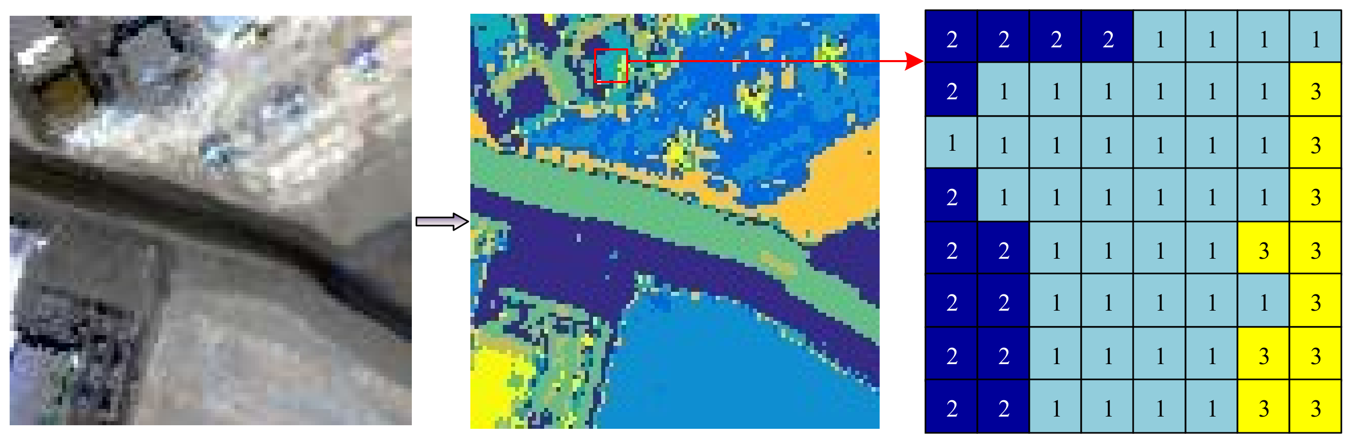
The -means clustering method [32] is used on the original dataset. The purpose is to generate a series of classes with spectral similarity. We assume that there are a total of classes (centroids) in the dataset, which is determined manually, mainly based on the complexity of the background components in the scene. If the HSI dataset consists of many types of background materials, should be set relatively large. Otherwise, it should be set as a small value. For an arbitrary pixel , if its class is , then the number of pixels belonging to in its eight-connected domain is counted. It can be considered that these pixels have high spectral similarity with . Furthermore, all of these pixels are connected in the spatial dimension. Thus, if the number of these pixels is larger than a threshold , then it is reasonable to determine the corresponding eight-connected domain as a background region. A schematic illustration is shown in Figure 3. Obviously, is related to the class number . If is relatively large, then the dataset will be clustered more fragmentarily, so should be set to a small value. If is small, the cluster map will be more integral, then should be set relatively large. Hence, we can conclude theoretically that and have an inverse relationship, and the product of them is a constant. In this letter, it is named the background constant , which is predefined in our method. Then, the threshold can be obtained as follows:
There are mainly two aspects that need to be taken into consideration to determine : (1) the number of eight-connected domains in the cluster map, which should be set relatively small if there exists a large number of eight-connected domains; and (2) the approximate sizes of anomalous targets in the scene. We can set as a large value if the targets are large, otherwise the value can be set to a small value.
Assume the cluster map can be segmented into non-overlapping eight-connected domains, denoted as . Each domain can be classified into the background domain set or the anomaly domain set based on the following rule:
where represents the pixel number of one certain domain. Suppose there are a total of domains in , denoted as , and the pixel number of each domain consists of a set . Pixels locating in can be deemed as background pixels with a high possibility. Then, an exponential weighting function is designed for these pixels:
where represents the minimal number in the set. The range of is , so every pixel in can be assigned an appropriate weight according to the domain to which they belong, and pixels belonging to a larger domain will have a smaller weight. Finally, the anomaly value for each pixel is updated as follows:
Equation (11) distinctly suppresses the response of background components owing to the cluster weighting item, which can make the detection result better.
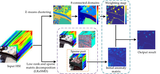
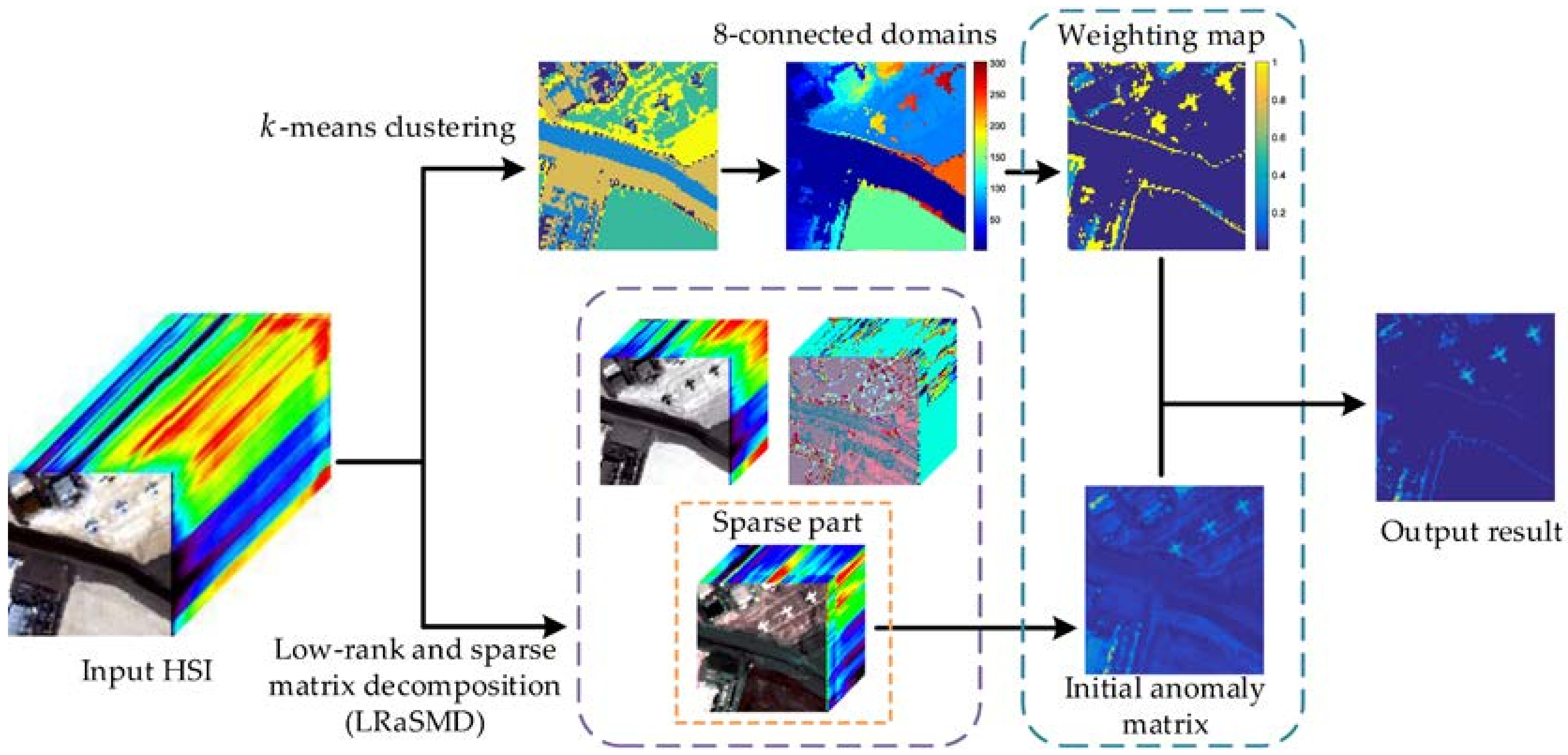
The proposed method is called LRaSMD with cluster weighting for anomaly detection (LSwCW). Its main procedure is summarized as Algorithm 1, and the corresponding flowchart is given in Figure 4.
| Algorithm 1 LRaSMD with cluster weighting for anomaly detection |
Input (1) The original HSI dataset ; (2) the upper bound of the rank ; (3) the sparsity level ; (4) the number of clustering centroids ; (5) the background constant .
|
3. Experimental Results and Analysis
3.1. Dataset Description
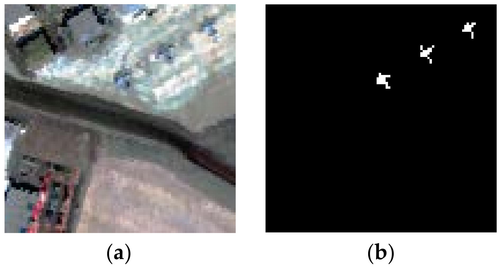
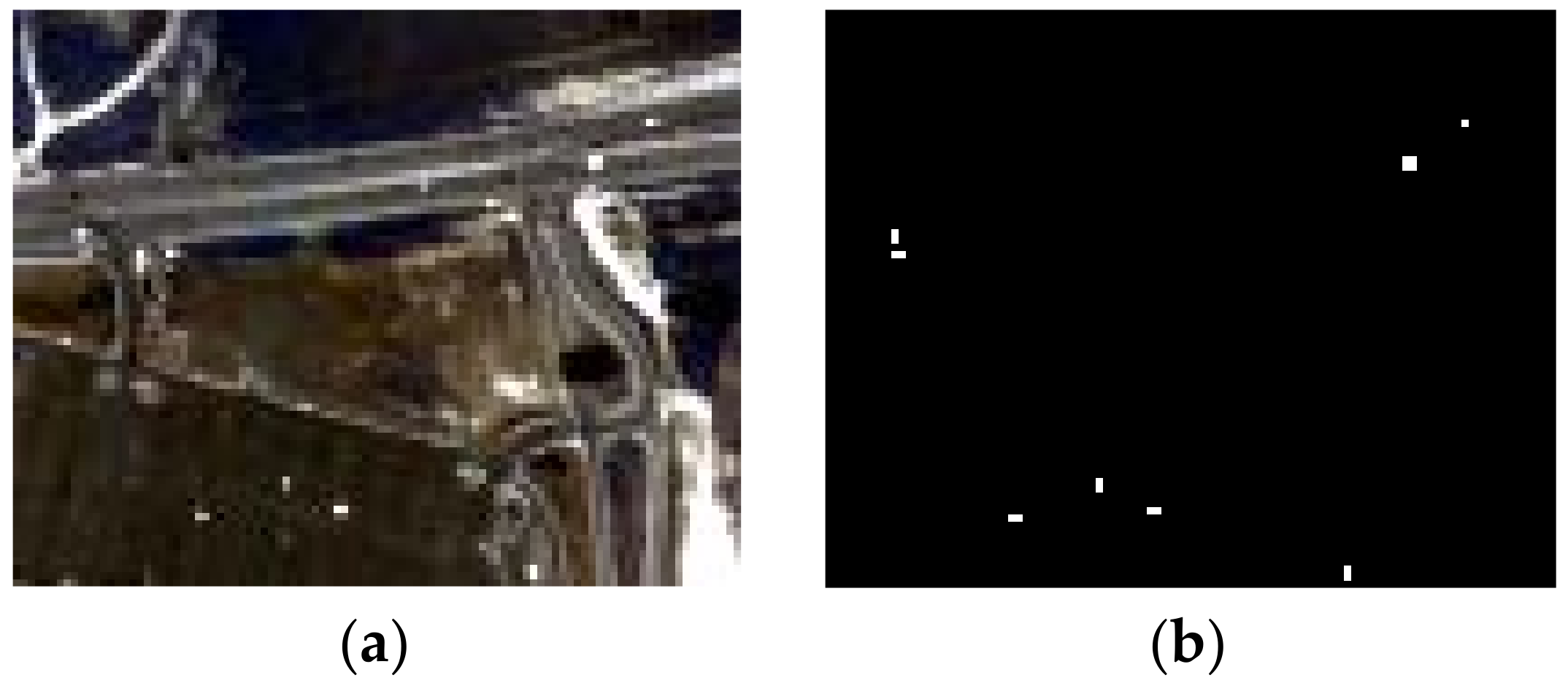
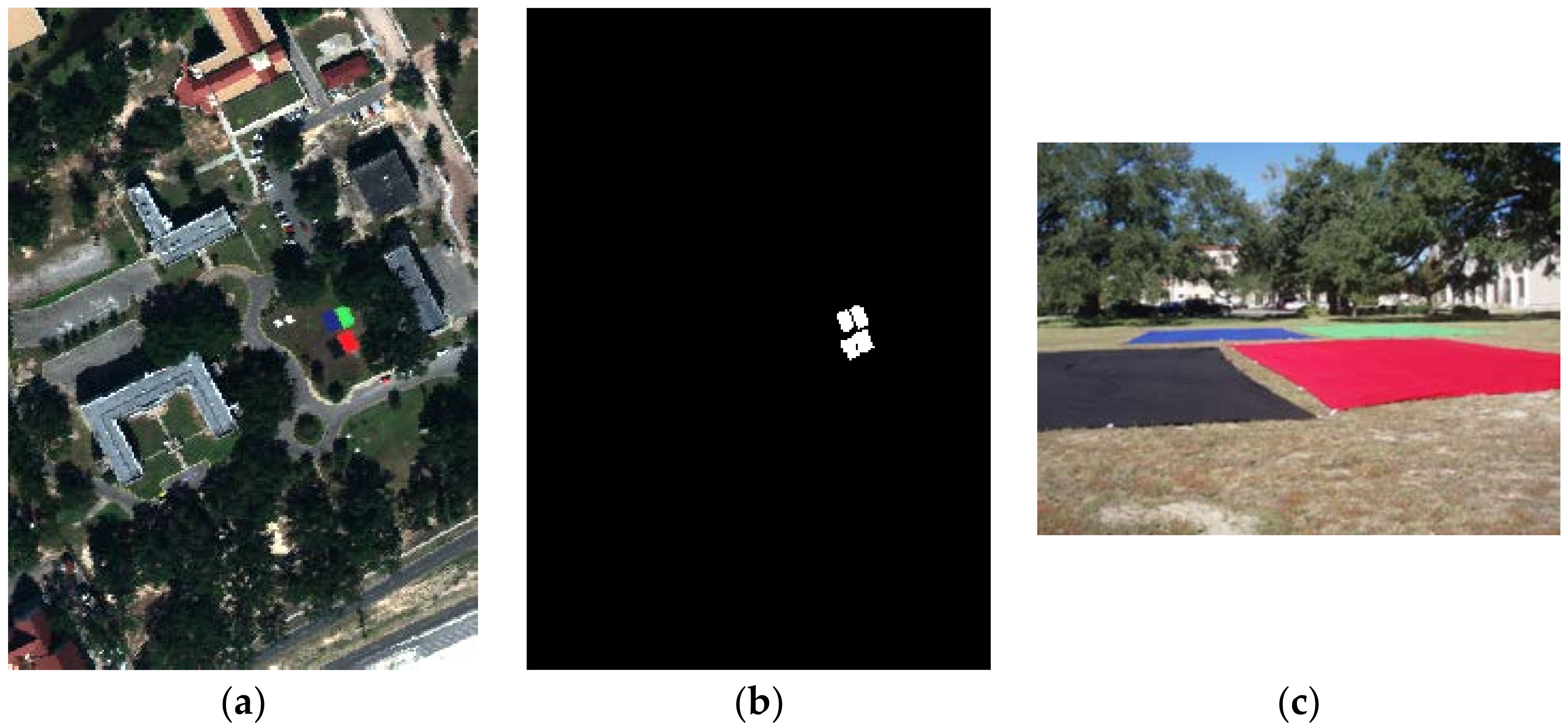
Three real HSI datasets are used to evaluate the effectiveness of the proposed method. The first was acquired by the Airborne Visible/Infrared Imaging Spectrometer (AVIRIS) sensor from the San Diego Airport, San Diego, CA, USA, with the size of 100 × 100 pixels. There are a total of 224 spectral bands ranging from 370–2510 nm. After eliminating the low-signal-to-noise ratio (SNR) and water vapor absorption bands, 189 bands are retained. Three airplanes in the scene, which contain 58 pixels, are considered as anomalous targets. The false color image and the ground-truth map are shown in Figure 5. The second is a Hyperspectral Digital Imagery Collection Experiment (HYDICE) dataset, which covers an urban area with a spectral resolution of 10 nm. It has 210 spectral bands in total, and 162 bands are used after removing the low-SNR and water vapor absorption bands. The size of the scene is 79 × 100 pixels; the false color image and the corresponding ground-truth map are shown in Figure 6. The third is the MUUFL Gulfport dataset, which is selected from the free hyperspectral datasets available to the remote sensing community [33,34,35,36,37]. It was collected in November 2010 over the University of Southern Mississippi Gulf Park Campus, located in Long Beach, Mississippi. The hyperspectral sensor has 72 spectral bands. Its wavelength range is 375–1050 nm, with a bandwidth of 10 nm. After removing the noise bands, there are 64 bands are used in the dataset, and the spatial size is 325 × 220. The RGB image of the dataset is shown in Figure 7a. Four cloth panels in the scene (see Figure 7c) are denoted as anomalous targets in our experiments. Their ground-truth map is given in Figure 7b.
3.2. Detection Performance
Several existing state-of-the-art anomaly detectors, including RX [9], kernel RX (KRX) [10], DWEST [15], CRD [17], and LRaSMD [22], are compared with our proposed LSwCW method to evaluate its performance. The experimental platform is a computer with an Intel Core i5-5200U central processing unit at 2.20 GHz and 12 GB random access memory. It is noteworthy that in all comparative experiments, the parameters of all algorithms are set as the optimal. A detailed parameter analysis of LSwCW will be described in the next subsection.
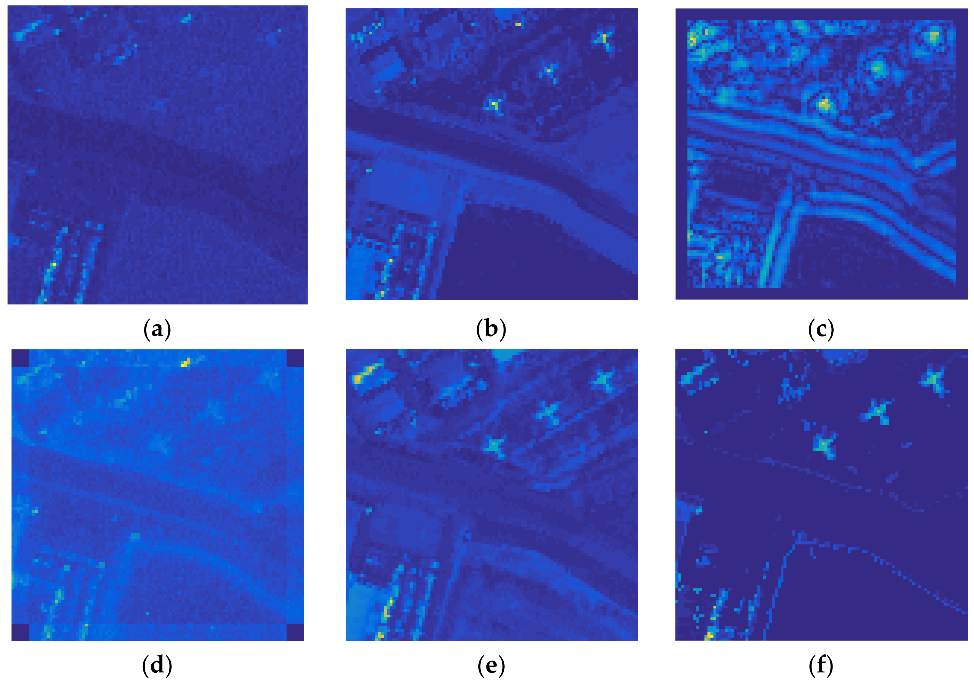
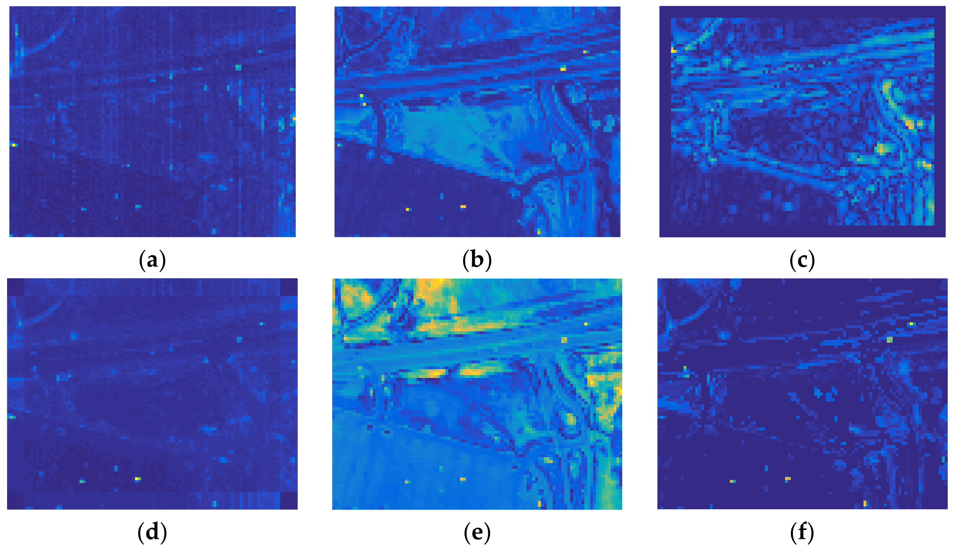
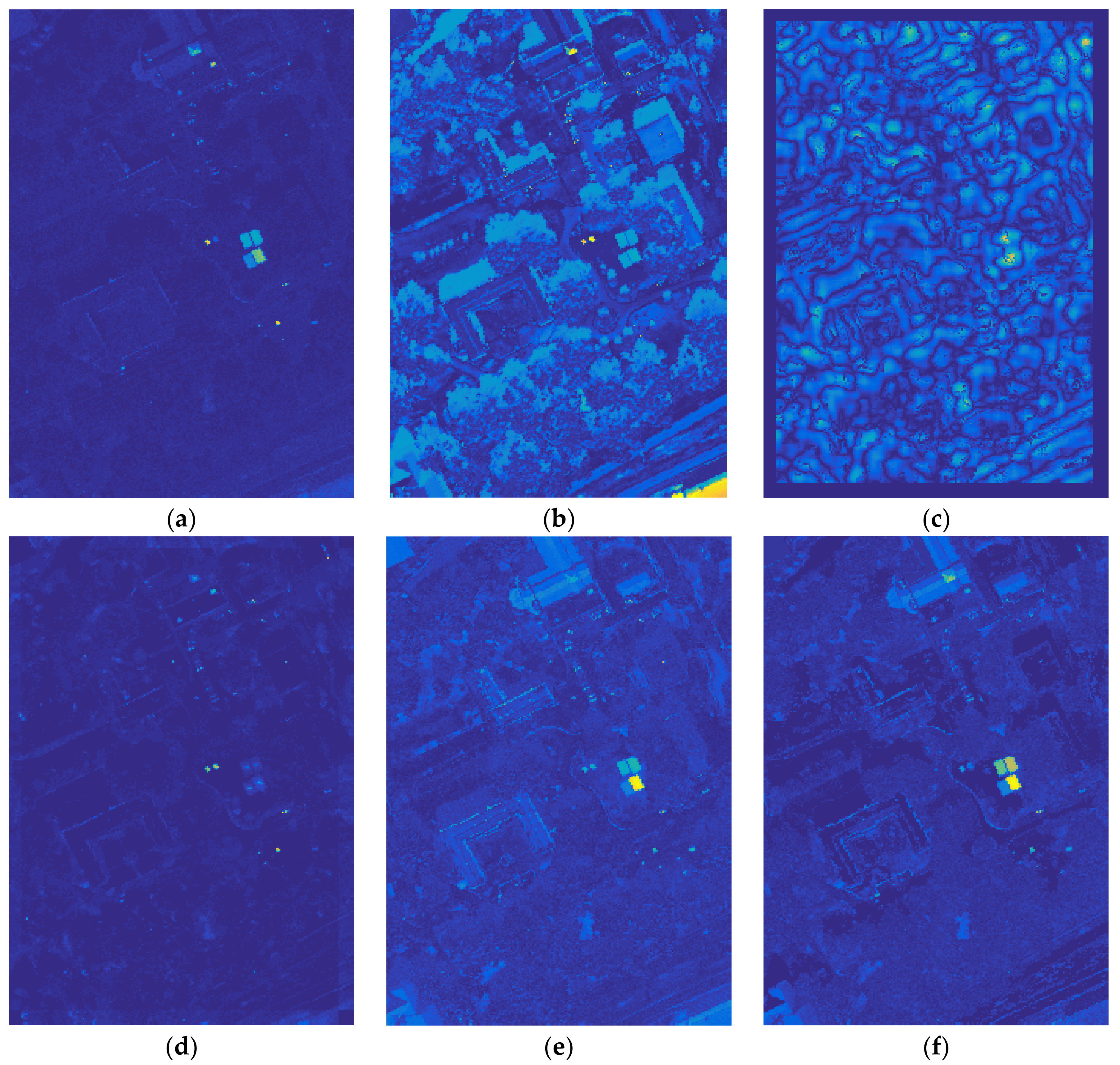
The color detection maps of compared algorithms for the AVIRIS dataset are represented in Figure 8. It can be seen that the anomalous targets are more distinguishable in the detection map of LSwCW when compared with the other results. Meanwhile, the homogeneous background can be well suppressed by LSwCW. For the HYDICE dataset, the detection result of each algorithm is shown in Figure 9. We can see that LSwCW suppresses most of background regions, and the true anomalous targets have high response values. Besides, RX, KRX, and CRD also provide good detection results, but a few anomaly pixels in these maps have low values, which influences their performances. For the MUUFL Gulfport dataset, the color detection maps of different algorithms are shown in Figure 10. The result of LSwCW reveals that anomalous targets can be effectively extracted by our proposed method, while the majority of the background can be suppressed. From other subfigures, we can see RX, CRD, and LRaSMD also obtain superior detection results, but in comparison, LSwCW is the best.
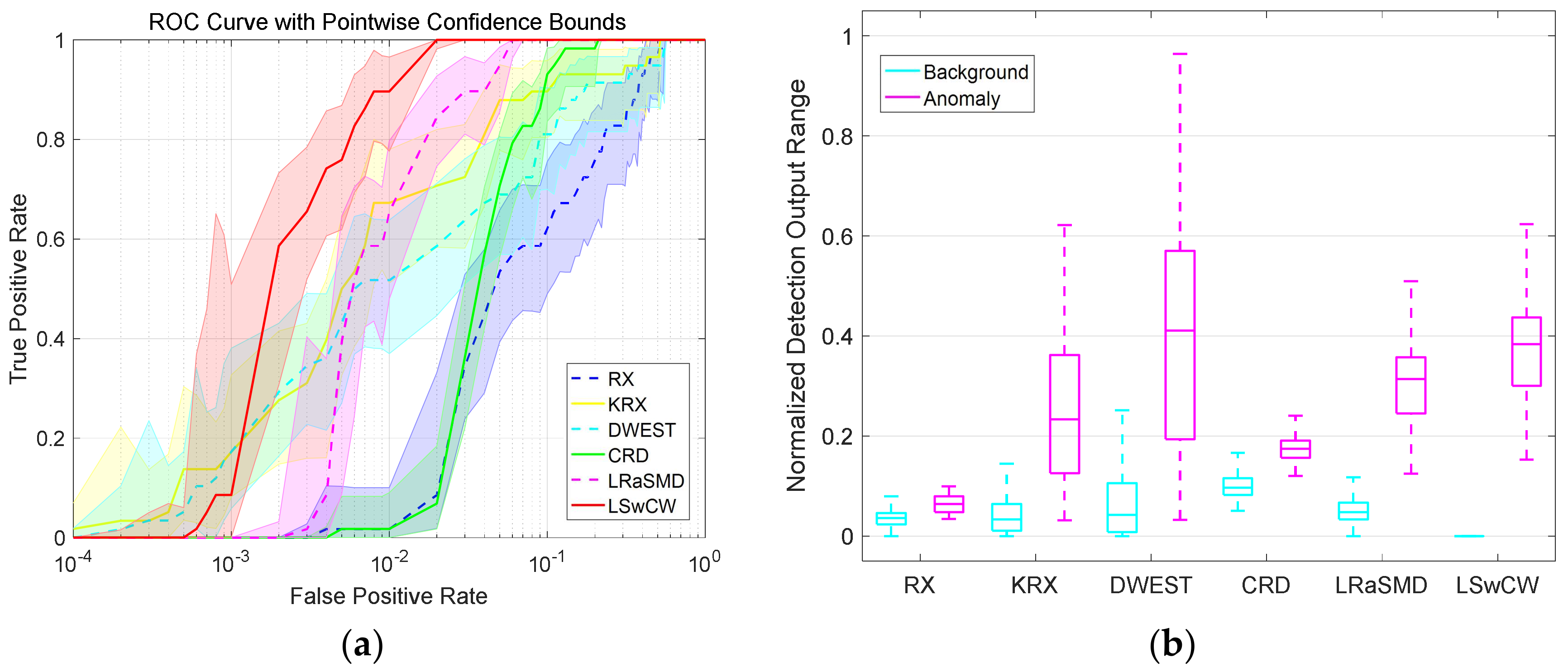
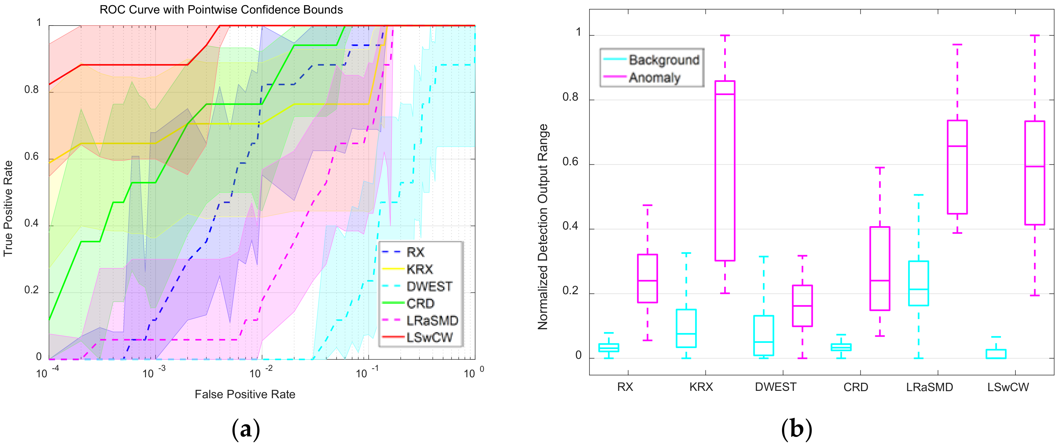
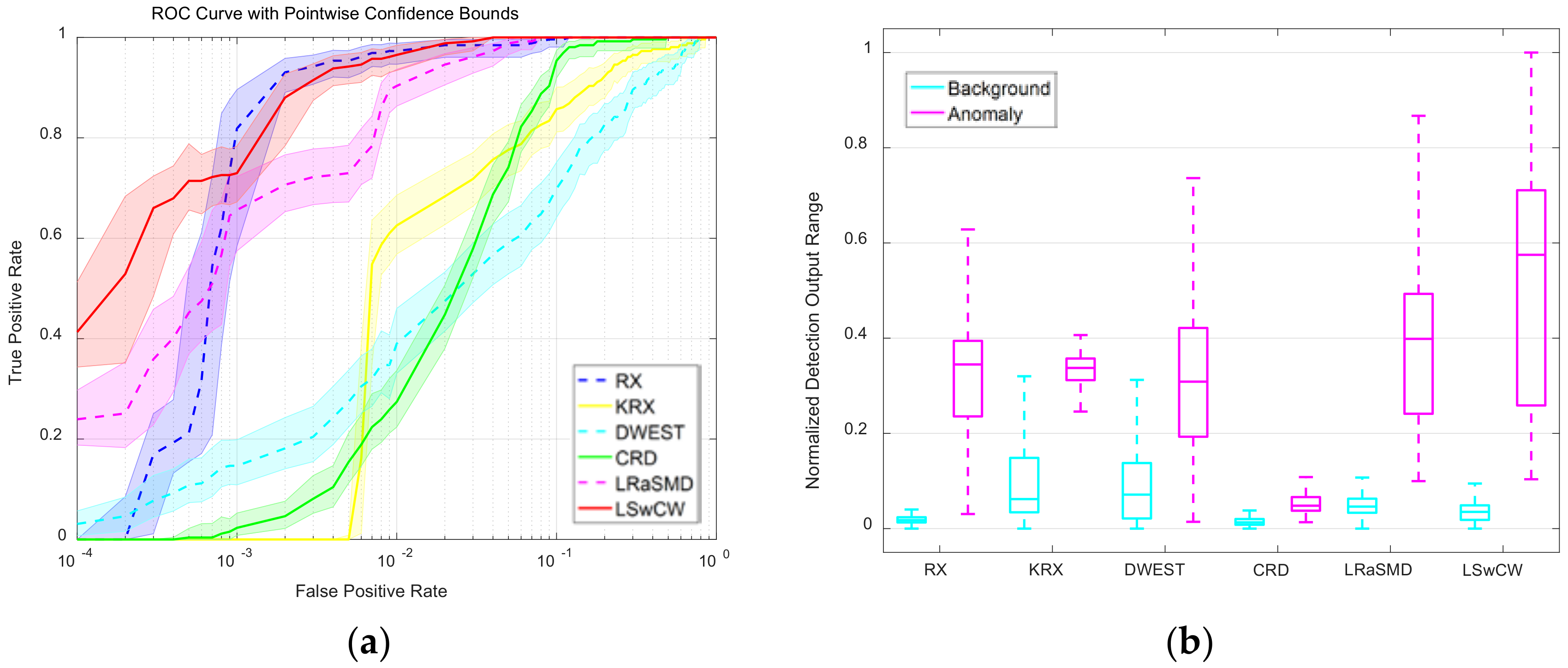
In order to further investigate the detection performance quantitatively, the receiver operating characteristic (ROC) curves with point-wise confidence intervals [38] are first provided. They are drawn on the log10 coordinate, and the point-wise confidence bounds are estimated based on bootstrap. Furthermore, the normalized background-anomaly separation maps are also utilized. For one specific detector, values of its detection map are first normalized to 0–1. Then two boxes are generated; the cyan box represents the value distribution of all background pixels, and the magenta box stands for the value distribution of all anomaly pixels. The central mark of the box indicates the median, while the bottom and top edges indicate the 25th and 75th percentiles, respectively. In addition, the whiskers extend to the most extreme data points not considered outliers. One detector has good separation performance if there exists an obvious gap between two boxes.
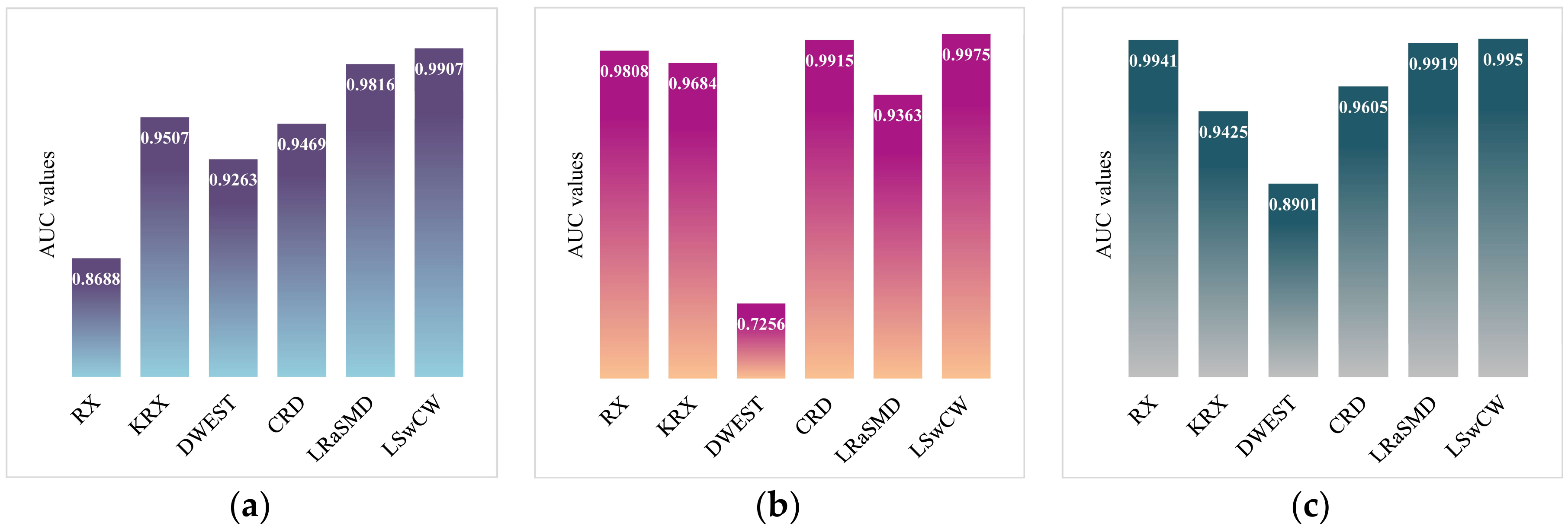
For the AVIRIS dataset, the ROC curves with point-wise confidence intervals are demonstrated in Figure 11a. As we can see, LSwCW obtains a remarkable ROC curve located at the upper-left corner of the figure, and its point-wise confidence bounds are always higher than the other detectors when the True Positive Rate (TPR) varies from 0 to 1. After it, LRaSMD and KRX also have better ROC curves with point-wise confidence intervals than the other algorithms. In addition, the normalized background-anomaly separation map of each algorithm is shown in Figure 11b. It can be seen that LSwCW suppresses the background information into a small value range, and discriminates anomalies from the background obviously. This proves that LSwCW has a superior separation performance compared to the other detection methods. For the HYDICE dataset, the quantitative evaluations are presented in Figure 12. From Figure 12a, we can see that the ROC curve of LSwCW is the best, and the corresponding confidence intervals are also higher than the others. According to the normalized background-anomaly separation map in Figure 12b, it can be observed that LSwCW has the best separation performance among the compared algorithms. The quantitative evaluation results of the MUUFL Gulfport dataset are demonstrated in Figure 13. The results of the ROC curves with point-wise confidence intervals and normalized background-anomaly separation map further illustrate that LSwCW has the most advanced detection performance compared with the other approaches. Furthermore, the area under the curve (AUC) values of each algorithm for the three datasets are reported in Figure 14a–c, respectively. From this figure, we can see that LSwCW has the highest AUC values in all three datasets, thus exhibiting outstanding detection performance. Finally, the computational costs of all compared algorithms for three datasets are listed in Table 1. The statistics reveal that LSwCW has high computational efficiency.
3.3. Parameter Sensitivity Analysis
There are four important parameters in LSwCW: the upper bound of the rank , the sparsity level , the number of clustering centroids , and the background constant . Experiments in this subsection are implemented on the AVIRIS, HYDICE, and MUUFL Gulfport datasets. In addition, when we analyze the specific parameter(s), the others are set to the optimal.
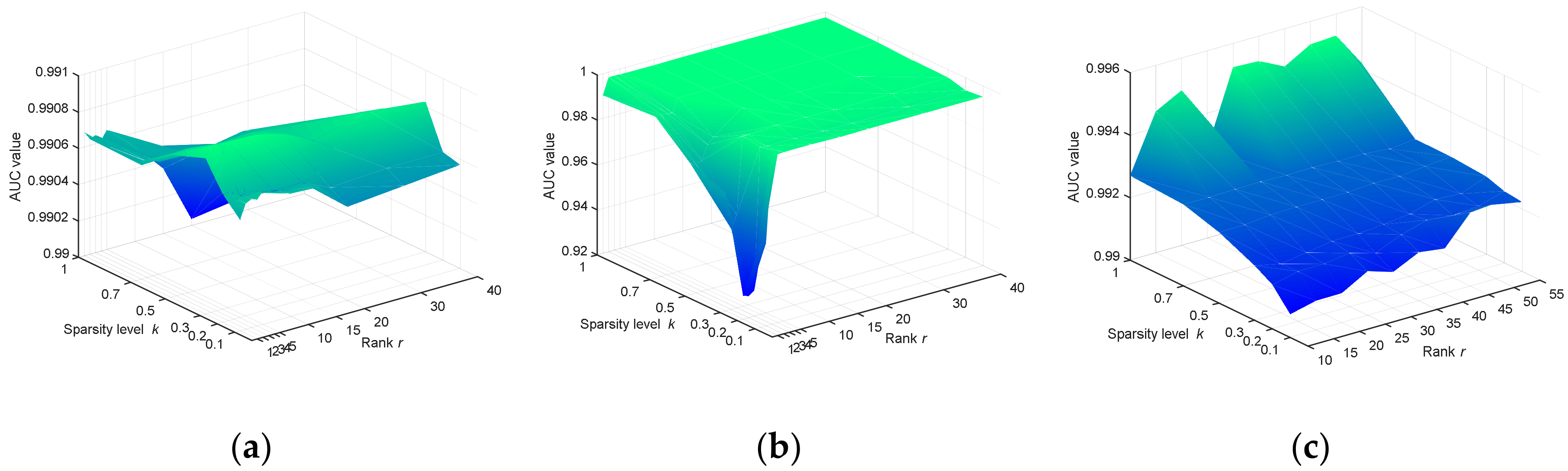
The rank is related to the main background materials in the scene. Without the loss of generality, for the AVIRIS and HYDICE datasets, the range of is set as (1, 2, 3, 4, 5, 10, 15, 20, 30, 40); for the MUUFL Gulfport dataset, it is set as (10, 15, 20, 25, 30, 35, 40, 45, 50, 55). In addition, the sparsity level is determined empirically, and all three datasets are set as (0.1, 0.2, 0.3, 0.5, 0.7, 1). For each dataset, the various detection performances with different combinations of and are exhibited by a three-dimensional (3D) plot, whose z-axis represents the corresponding AUC value. As shown in Figure 15, for the AVIRIS dataset, the AUC values are higher than 0.99 with any combinations of and , which reflects the robustness of LSwCW to the transformations of these two parameters. For the HYDICE dataset, the AUC values are relatively low when is less than 3 and is lower than 0.3 simultaneously. On other positions, it can achieve a high value over 0.99. This may be because the HYDICE dataset has complex background components, which should be described satisfactorily by more than three basis spectral vectors. Therefore, the rank should be relatively large. Moreover, some anomaly pixels may be mixed by background spectra with high proportions, so it is necessary to set in a relatively high value to detect them. For the MUUFL Gulfport dataset, the AUC values are high and stable with the change of and , especially when the sparsity level is larger than 0.7. This is because the cloth panel on the lower left is quite similar to the background of grass, so should be enlarged to extract it effectively.
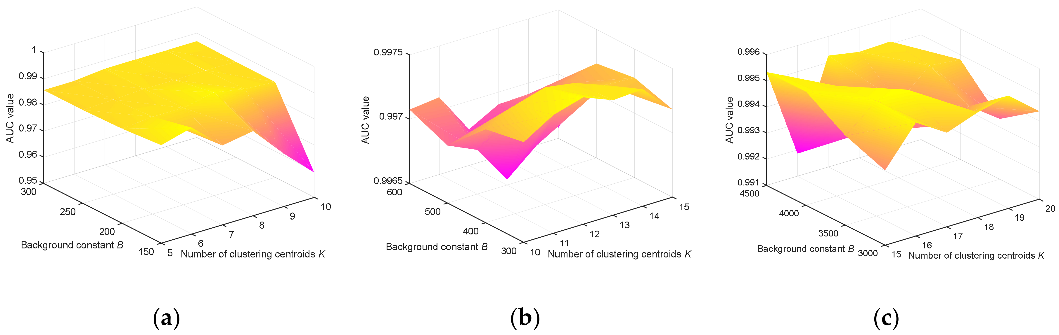
The parameter can be set based on the number of main background materials in the image. The background constant is selected empirically, and usually is an integer multiple of . Considering the difference of the main background categories in the three datasets, for the AVIRIS dataset, is set from 5 to 10, and ranges from 150 to 300, with a step interval of 50. For the HYDICE dataset, the value range of is 10 to 15, while is 300 to 600, with a step interval of 100. For the MUUFL Gulfport dataset, is set from 15 to 20, and is set as (3000, 3500, 4000, 4500). The results are also demonstrated by using 3D plots, which are shown in Figure 16. In general, LSwCW is quite robust to the parameters and . Only in one case, in which is large while is too small, is the detection performance relatively weak, because this situation can lead to a small value of threshold , which may misclassify the anomaly cluster as background.
4. Discussion
In the basis of the experimental results and the relevant parameter analyses, it can be considered that our proposed method has preeminent performance in terms of various evaluation indicators. Firstly, some state-of-the-art anomaly detectors are chosen as comparison algorithms. They are RX, KRX, DWEST, CRD, and LRaSMD. Among them, the RX detector is a well-known benchmark anomaly detection algorithm. The KRX detector is a nonlinear version of RX, which has been proven to be a superior algorithm. The DWEST represents the type of algorithms that utilize the dual window strategy. The CRD is one of the most typical representation-based methods. Finally, the LRaSMD is selected as a comparison algorithm since it uses the same technique as our proposed method. The qualitative analyses of different algorithms for the three datasets are demonstrated by color detection maps, which are shown in Figure 8, Figure 9 and Figure 10. These three figures indicate intuitively the good detection results of LSwCW. Compared with the other methods, LSwCW can well suppress background pixels because of the cluster weighting strategy. Meanwhile, anomaly pixels can be extracted obviously owing to the procedure of low-rank and sparse matrix decomposition. The quantitative analyses are given through ROC curves with point-wise confidence intervals, AUC values, as well as normalized background-anomaly separation maps. The better detector has an ROC curve which is closer to the upper-left corner, and the point-wise confidence bounds are higher in the case of the equal False Positive Rate (FPR). In addition, the corresponding AUC value is larger. Moreover, its background box and the anomaly box have a larger gap in the normalized background-anomaly separation map. The quantitative comparison results are depicted in Figure 11, Figure 12, Figure 13 and Figure 14. According to the aforementioned evaluation standards, LSwCW has the best ROC curves with point-wise confidence intervals for the three datasets, and its AUC values are the largest. Furthermore, the normalized background-anomaly separation maps also confirm the best separation performance of LSwCW in all compared algorithms. We also measured the computational cost of each algorithm, which is reported in Table 1. It can be seen that LSwCW is not the fastest, but its time consumptions still lie in the acceptable range for real applications. We believe that the computational efficiency can be further improved through optimizing codes.
Determining suitable parameters is important to obtain good detection results. To judge the capability of one algorithm, it is necessary to analyze its sensitivity to the transformations of different parameters. In our experiments, this is evaluated by changing four essential parameters: (1) the upper bound of the rank ; (2) the sparsity level ; (3) the number of clustering centroids ; and (4) the background constant . All parameters are set to large value ranges; then, we combine two parameters together, and obtain the 3D plots. They are illustrated in Figure 15 and Figure 16, respectively. It can be seen that LSwCW is quite robust with regard to the parameters’ transformations. Only in a few special cases are the AUC values reduced, and the reasons for these phenomena were explained in detail in Section 3.3.
Although our proposed method yields an outstanding detection performance, there still exist some aspects which can be further investigated. For instance, the empirical parameters may influence the detection performance if they are set outside reasonable ranges. In the future, we will focus on how to determine all parameters automatically and adaptively, and we believe this will further improve the practicality of this method.
5. Conclusions
Detecting anomalous targets precisely and reliably from HSIs is an important research issue in hyperspectral remote sensing. Considering anomalies’ low probability of occurrence, significant spectral difference from main background materials, and spatial distribution characteristics, a new anomaly detection approach named LSwCW is proposed in this letter. The GoDec algorithm is first applied to decompose the original dataset to the low-rank part, the sparse part, and the noise part. The initial anomaly matrix is then obtained by calculating the -norm for each pixel on the sparse matrix. To suppress the responses of background pixels, especially background regions with a sparse property, a cluster weighting strategy is utilized. Finally, the anomaly matrix is updated, which is denoted as the detection result. LSwCW makes full use of the sparse property of anomalies and extracts them based on the spectral difference. Meanwhile, the spatial distribution characteristics of anomalies and the background are also taken into account, which can make the result more accurate. Experimental results on three real-world HSI datasets showed the effectiveness, robustness, and low computation time of the proposed method.
Author Contributions
L.Z. proposed the general idea of the method, as well as designed and performed the experiments. G.W. provided constructive and beneficial advice for the preparation. G.W. and S.Q. supervised the study and reviewed this paper. This paper was written by L.Z.
Acknowledgments
The work is supported in part by the Program for New Century Excellent Talents in the University of China under Grants NCET-11-0866 and in part by the National Natural Science Foundation of China under Grants 41601487.
Conflicts of Interest
The authors declare no conflict of interest.
References
- Bioucas-Dias, J.M.; Plaza, A.; Camps-Valls, G.; Scheunders, P.; Nasrabadi, N.; Chanussot, J. Hyperspectral remote sensing data analysis and future challenges. IEEE Geosci. Remote Sens. Mag. 2013, 1, 6–36. [Google Scholar] [CrossRef]
- Manolakis, D.; Truslow, E.; Pieper, M.; Cooley, T.; Brueggeman, M. Detection algorithms in hyperspectral imaging systems: An overview of practical algorithms. IEEE Signal Process. Mag. 2014, 31, 24–33. [Google Scholar] [CrossRef]
- Matteoli, S.; Diani, M.; Corsini, G. A tutorial overview of anomaly detection in hyperspectral images. IEEE Aerosp. Electr. Syst. Mag. 2010, 25, 5–28. [Google Scholar] [CrossRef]
- Stein, D.W.; Beaven, S.G.; Hoff, L.E.; Winter, E.M.; Schaum, A.P.; Stocker, A.D. Anomaly detection from hyperspectral imagery. IEEE Signal Process. Mag. 2002, 19, 58–69. [Google Scholar] [CrossRef]
- Manolakis, D. Detection algorithms for hyperspectral imaging applications: A signal processing perspective. In Proceedings of the 2003 IEEE Workshop on Advances in Techniques for Analysis of Remotely Sensed Data, Greenbelt, MD, USA, 27–28 October 2003; pp. 378–384. [Google Scholar]
- Manolakis, D.; Lockwood, R.; Cooley, T.; Jacobson, J. Is there a best hyperspectral detection algorithm? SPIE Proc. 2009, 7334, 733402. [Google Scholar] [CrossRef]
- Manolakis, D.; Marden, D.; Shaw, G.A. Hyperspectral image processing for automatic target detection applications. Lincoln Lab. J. 2003, 14, 79–116. [Google Scholar]
- Zhu, L.; Wen, G. Hyperspectral anomaly detection via background estimation and adaptive weighted sparse representation. Remote Sens. 2018, 10, 272. [Google Scholar] [CrossRef]
- Reed, I.S.; Yu, X. Adaptive multiple-band cfar detection of an optical pattern with unknown spectral distribution. IEEE Trans. Acoust. Speech Signal Process. 1990, 38, 1760–1770. [Google Scholar] [CrossRef]
- Kwon, H.; Nasrabadi, N.M. Kernel rx-algorithm: A nonlinear anomaly detector for hyperspectral imagery. IEEE Trans. Geosci. Remote Sens. 2005, 43, 388–397. [Google Scholar] [CrossRef]
- Zhou, J.; Kwan, C.; Ayhan, B.; Eismann, M.T. A novel cluster kernel rx algorithm for anomaly and change detection using hyperspectral images. IEEE Trans. Geosci. Remote Sens. 2016, 54, 6497–6504. [Google Scholar] [CrossRef]
- Schaum, A. Joint subspace detection of hyperspectral targets. In Proceedings of the 2014 IEEE Aerospace Conference, Big Sky, MT, USA, 6–13 March 2004. [Google Scholar]
- Guo, Q.; Zhang, B.; Ran, Q.; Gao, L.; Li, J.; Plaza, A. Weighted-rxd and linear filter-based rxd: Improving background statistics estimation for anomaly detection in hyperspectral imagery. IEEE J. Sel. Top. Appl. Earth Observ. Remote Sens. 2014, 7, 2351–2366. [Google Scholar] [CrossRef]
- Carlotto, M.J. A cluster-based approach for detecting man-made objects and changes in imagery. IEEE Trans. Geosci. Remote Sens. 2005, 43, 374–387. [Google Scholar] [CrossRef]
- Kwon, H.; Der, S.Z.; Nasrabadi, N.M. Adaptive anomaly detection using subspace separation for hyperspectral imagery. Opt. Eng. 2003, 42, 3342–3351. [Google Scholar] [CrossRef]
- Billor, N.; Hadi, A.S.; Velleman, P.F. Bacon: Blocked adaptive computationally efficient outlier nominators. Comput. Stat. Data Anal. 2000, 34, 279–298. [Google Scholar] [CrossRef]
- Li, W.; Du, Q. Collaborative representation for hyperspectral anomaly detection. IEEE Trans. Geosci. Remote Sens. 2015, 53, 1463–1474. [Google Scholar] [CrossRef]
- Veracini, T.; Matteoli, S.; Diani, M.; Corsini, G. Fully unsupervised learning of gaussian mixtures for anomaly detection in hyperspectral imagery. In Proceedings of the 2009 Ninth International Conference on Intelligent Systems Design and Applications, Pisa, Italy, 30 November–2 December 2009; pp. 596–601. [Google Scholar]
- Adler-Golden, S.M. Improved hyperspectral anomaly detection in heavy-tailed backgrounds. In Proceedings of the 2009 First Workshop on Hyperspectral Image and Signal Processing: Evolution in Remote Sensing, Grenoble, France, 26–28 August 2009; pp. 1–4. [Google Scholar]
- Qu, Y.; Guo, R.; Wang, W.; Qi, H.; Ayhan, B.; Kwan, C.; Vance, S. Anomaly detection in hyperspectral images through spectral unmixing and low rank decomposition. In Proceedings of the 2016 IEEE International Geoscience and Remote Sensing Symposium (IGARSS), Beijing, China, 10–15 July 2016; pp. 1855–1858. [Google Scholar]
- Wang, W.; Li, S.; Qi, H.; Ayhan, B.; Kwan, C.; Vance, S. Identify anomaly componentbysparsity and low rank. In Proceedings of the 2015 7th Workshop on Hyperspectral Image and Signal Processing: Evolution in Remote Sensing (WHISPERS), Tokyo, Japan, 2–5 June 2015; pp. 1–4. [Google Scholar]
- Sun, W.; Liu, C.; Li, J.; Lai, Y.M.; Li, W. Low-rank and sparse matrix decomposition-based anomaly detection for hyperspectral imagery. J. Appl. Remote Sens. 2014, 8, 083641. [Google Scholar] [CrossRef]
- Zhang, Y.; Du, B.; Zhang, L.; Wang, S. A low-rank and sparse matrix decomposition-based mahalanobis distance method for hyperspectral anomaly detection. IEEE Trans. Geosci. Remote Sens. 2016, 54, 1376–1389. [Google Scholar] [CrossRef]
- Cui, X.; Tian, Y.; Weng, L.; Yang, Y. Anomaly detection in hyperspectral imagery based on low-rank and sparse decomposition. SPIE Proc. 2014, 9069. [Google Scholar] [CrossRef]
- Golbabaee, M.; Vandergheynst, P. Hyperspectral image compressed sensing via low-rank and joint-sparse matrix recovery. In Proceedings of the 2012 IEEE International Conference on Acoustics, Speech and Signal Processing (ICASSP), Kyoto, Japan, 25–30 March 2012; pp. 2741–2744. [Google Scholar]
- Xiong, L.; Chen, X.; Schneider, J. Direct robust matrix factorizatoin for anomaly detection. In Proceedings of the 2011 IEEE 11th International Conference on Data Mining (ICDM), Vancouver, BC, Canada, 11–14 December 2011; pp. 844–853. [Google Scholar]
- Halko, N.; Martinsson, P.-G.; Tropp, J.A. Finding Structure with Randomness: Stochastic Algorithms for Constructing Approximate Matrix Decompositions; California Institute of Technology: Pasadena, CA, USA, 2009. [Google Scholar]
- Candes, E.J.; Li, X.; Wright, J.; Ma, Y. Robust Principal Component Analysis? J. ACM 2011, 58, 11. [Google Scholar] [CrossRef]
- Zhou, T.; Tao, D. Godec: Randomized low-rank & sparse matrix decomposition in noisy case. In Proceedings of the International Conference on Machine Learning, Bellevue, WA, USA, 28 June–2 July 2011; Omnipress: Madison, WI, USA, 2011. [Google Scholar]
- Chen, Y.; Nasrabadi, N.M.; Tran, T.D. Hyperspectral image classification using dictionary-based sparse representation. IEEE Trans. Geosci. Remote Sens. 2011, 49, 3973–3985. [Google Scholar] [CrossRef]
- Dao, M.; Kwan, C.; Koperski, K.; Marchisio, G. A joint sparsity approach to tunnel activity monitoring using high resolution satellite images. In Proceedings of the IEEE Ubiquitous Computing, Electronics and Mobile Communication Conference, New York City, NY, USA, 19–21 October 2017. [Google Scholar]
- Jain, A.K.; Murty, M.N.; Flynn, P.J. Data clustering: A review. ACM Comput. Surv. 1999, 31, 264–323. [Google Scholar] [CrossRef]
- Gader, P.; Zare, A.; Close, R.; Aitken, J.; Tuell, G. Muufl Gulfport Hyperspectral and Lidar Airborne Data Set; Technical Report, REP-2013-570; University of Florida: Gainesville, FL, USA, 2013. [Google Scholar]
- Snyder, D.; Kerekes, J.; Fairweather, I.; Crabtree, R.; Shive, J.; Hager, S. Development of a web-based application to evaluate target finding algorithms. In Proceedings of the 2008 IEEE International Geoscience and Remote Sensing Symposium, Boston, MA, USA, 7–11 July 2008; pp. II-915–II-918. [Google Scholar]
- Herweg, J.A.; Kerekes, J.P.; Weatherbee, O.; Messinger, D.; van Aardt, J.; Ientilucci, E.; Ninkov, Z.; Faulring, J.; Raqueño, N.; Meola, J. Spectir hyperspectral airborne rochester experiment data collection campaign. SPIE Proc. 2012, 8390. [Google Scholar] [CrossRef]
- Giannandrea, A.; Raqueno, N.; Messinger, D.W.; Faulring, J.; Kerekes, J.P.; van Aardt, J.; Canham, K.; Hagstrom, S.; Ontiveros, E.; Gerace, A. The SHARE 2012 data campaign. SPIE Proc. 2013, 8743. [Google Scholar] [CrossRef]
- Acito, N.; Matteoli, S.; Rossi, A.; Diani, M.; Corsini, G. Hyperspectral airborne “viareggio 2013 trial” data collection for detection algorithm assessment. IEEE J. Sel. Top. Appl. Earth Observ. Remote Sens. 2016, 9, 2365–2376. [Google Scholar] [CrossRef]
- Kerekes, J. Receiver operating characteristic curve confidence intervals and regions. IEEE Geosci. Remote Sens. Lett. 2008, 5, 251–255. [Google Scholar] [CrossRef]
Figure 1.
Decomposed data cubes of an HSI dataset by using the low-rank and sparse matrix decomposition (LRaSMD) technique. (a) Low-rank part; (b) sparse part; (c) noise part.
Figure 1.
Decomposed data cubes of an HSI dataset by using the low-rank and sparse matrix decomposition (LRaSMD) technique. (a) Low-rank part; (b) sparse part; (c) noise part.

Figure 2.
An example to demonstrate the high values of background regions with sparse property on the initial anomaly matrix.
Figure 2.
An example to demonstrate the high values of background regions with sparse property on the initial anomaly matrix.

Figure 3.
Schematic illustration of the judgement of background regions. The eight-connected domain labeled with 1 can be considered as the background.
Figure 3.
Schematic illustration of the judgement of background regions. The eight-connected domain labeled with 1 can be considered as the background.

Figure 4.
Schematic flowchart of the proposed LRaSMD with cluster weighting (LSwCW) anomaly detection method.
Figure 4.
Schematic flowchart of the proposed LRaSMD with cluster weighting (LSwCW) anomaly detection method.

Figure 5.
Airborne Visible/Infrared Imaging Spectrometer (AVIRIS) dataset. (a) False color image; (b) ground-truth map.
Figure 5.
Airborne Visible/Infrared Imaging Spectrometer (AVIRIS) dataset. (a) False color image; (b) ground-truth map.

Figure 6.
Hyperspectral Digital Imagery Collection Experiment (HYDICE) dataset. (a) False color image; (b) ground-truth map.
Figure 6.
Hyperspectral Digital Imagery Collection Experiment (HYDICE) dataset. (a) False color image; (b) ground-truth map.

Figure 7.
MUUFL Gulfport dataset. (a) RGB image; (b) ground-truth map; (c) anomalous targets.

Figure 8.
Color detection maps of compared algorithms for the AVIRIS dataset. (a) Reed-Xiaoli detector (RX); (b) kernel RX (KRX); (c) dual window-based eigen separation transform detector (DWEST); (d) collaborative representation-based detector (CRD); (e) low-rank and sparse matrix decomposition-based detector (LRaSMD); (f) LRaSMD with cluster weighting-based detector (LSwCW).

Figure 9.
Color detection maps of compared algorithms for the HYDICE dataset. (a) RX; (b) KRX; (c) DWEST; (d) CRD; (e) LRaSMD; (f) LSwCW.
Figure 9.
Color detection maps of compared algorithms for the HYDICE dataset. (a) RX; (b) KRX; (c) DWEST; (d) CRD; (e) LRaSMD; (f) LSwCW.

Figure 10.
Color detection maps of compared algorithms for the MUUFL Gulfport dataset. (a) RX; (b) KRX; (c) DWEST; (d) CRD; (e) LRaSMD; (f) LSwCW.
Figure 10.
Color detection maps of compared algorithms for the MUUFL Gulfport dataset. (a) RX; (b) KRX; (c) DWEST; (d) CRD; (e) LRaSMD; (f) LSwCW.

Figure 11.
Quantitative evaluations for different algorithms for the AVIRIS dataset. (a) Receiver operating characteristic (ROC) curves with point-wise confidence intervals; (b) normalized background-anomaly separation map.
Figure 11.
Quantitative evaluations for different algorithms for the AVIRIS dataset. (a) Receiver operating characteristic (ROC) curves with point-wise confidence intervals; (b) normalized background-anomaly separation map.

Figure 12.
Quantitative evaluations for different algorithms for the HYDICE dataset. (a) ROC curves with point-wise confidence intervals; (b) normalized background-anomaly separation map.
Figure 12.
Quantitative evaluations for different algorithms for the HYDICE dataset. (a) ROC curves with point-wise confidence intervals; (b) normalized background-anomaly separation map.

Figure 13.
Quantitative evaluations for different algorithms for the MUUFL Gulfport dataset. (a) ROC curves with point-wise confidence intervals; (b) normalized background-anomaly separation map.
Figure 13.
Quantitative evaluations for different algorithms for the MUUFL Gulfport dataset. (a) ROC curves with point-wise confidence intervals; (b) normalized background-anomaly separation map.

Figure 14.
Area under the curve (AUC) values of compared algorithms for different datasets. (a) AVIRIS dataset; (b) HYDICE dataset; (c) MUUFL Gulfport dataset.
Figure 14.
Area under the curve (AUC) values of compared algorithms for different datasets. (a) AVIRIS dataset; (b) HYDICE dataset; (c) MUUFL Gulfport dataset.

Figure 15.
AUC illustration with the transformations of the rank and the sparsity level on three datasets. (a) AVIRIS dataset; (b) HYDICE dataset; (c) MUUFL Gulfport dataset.
Figure 15.
AUC illustration with the transformations of the rank and the sparsity level on three datasets. (a) AVIRIS dataset; (b) HYDICE dataset; (c) MUUFL Gulfport dataset.

Figure 16.
AUC illustration with the transformations of the number of clustering centroids and the background constant on three datasets. (a) AVIRIS dataset; (b) HYDICE dataset; (c) MUUFL Gulfport dataset.
Figure 16.
AUC illustration with the transformations of the number of clustering centroids and the background constant on three datasets. (a) AVIRIS dataset; (b) HYDICE dataset; (c) MUUFL Gulfport dataset.


Table 1.
Computational costs of different algorithms for the AVIRIS, HYDICE, and MUUFL Gulfport datasets.
Table 1.
Computational costs of different algorithms for the AVIRIS, HYDICE, and MUUFL Gulfport datasets.
| Time (s) | RX | KRX | DWEST | CRD | LRaSMD | LSwCW |
|---|---|---|---|---|---|---|
| AVIRIS | 0.24 | 1.74 | 57.74 | 87.94 | 0.78 | 3.41 |
| HYDICE | 0.38 | 1.35 | 46.32 | 68.46 | 0.45 | 2.25 |
| MUUFL Gulfport | 0.65 | 23.12 | 1292.32 | 541.05 | 2.03 | 17.17 |
© 2018 by the authors. Licensee MDPI, Basel, Switzerland. This article is an open access article distributed under the terms and conditions of the Creative Commons Attribution (CC BY) license (http://creativecommons.org/licenses/by/4.0/).
Share and Cite
MDPI and ACS Style
Zhu, L.; Wen, G.; Qiu, S. Low-Rank and Sparse Matrix Decomposition with Cluster Weighting for Hyperspectral Anomaly Detection. Remote Sens. 2018, 10, 707. https://0-doi-org.brum.beds.ac.uk/10.3390/rs10050707
AMA Style
Zhu L, Wen G, Qiu S. Low-Rank and Sparse Matrix Decomposition with Cluster Weighting for Hyperspectral Anomaly Detection. Remote Sensing. 2018; 10(5):707. https://0-doi-org.brum.beds.ac.uk/10.3390/rs10050707
Chicago/Turabian StyleZhu, Lingxiao, Gongjian Wen, and Shaohua Qiu. 2018. "Low-Rank and Sparse Matrix Decomposition with Cluster Weighting for Hyperspectral Anomaly Detection" Remote Sensing 10, no. 5: 707. https://0-doi-org.brum.beds.ac.uk/10.3390/rs10050707
Note that from the first issue of 2016, this journal uses article numbers instead of page numbers. See further details here.