Speckle Suppression by Weighted Euclidean Distance Anisotropic Diffusion


1
State Key Laboratory of Information Engineering in Surveying Mapping and Remote Sensing, Wuhan University, Wuhan 430079, China
2
Collaborative Innovation Center of Geospatial Technology, Wuhan University, Wuhan 430079, China
3
China Academy of Space Technology, Beijing 100094, China
4
School of Geomatics, Liaoning Technical University, Fuxin 123000, China
5
School of Remote Sensing and Information Engineering, Wuhan University, Wuhan 430079, China
*
Author to whom correspondence should be addressed.
Remote Sens. 2018, 10(5), 722; https://0-doi-org.brum.beds.ac.uk/10.3390/rs10050722
Submission received: 21 April 2018
/
Revised: 5 May 2018
/
Accepted: 7 May 2018
/
Published: 8 May 2018
(This article belongs to the Section Remote Sensing Image Processing)
Abstract
:To better reduce image speckle noise while also maintaining edge information in synthetic aperture radar (SAR) images, we propose a novel anisotropic diffusion algorithm using weighted Euclidean distance (WEDAD). Presented here is a modified speckle reducing anisotropic diffusion (SRAD) method, which constructs a new edge detection operator using weighted Euclidean distances. The new edge detection operator can adaptively distinguish between homogenous and heterogeneous image regions, effectively generate anisotropic diffusion coefficients for each image pixel, and filter each pixel at different scales. Additionally, the effects of two different weighting methods (Gaussian weighting and non-linear weighting) of de-noising were analyzed. The effect of different adjustment coefficient settings on speckle suppression was also explored. A series of experiments were conducted using an added noise image, GF-3 SAR image, and YG-29 SAR image. The experimental results demonstrate that the proposed method can not only significantly suppress speckle, thus improving the visual effects, but also better preserve the edge information of images.
1. Introduction
Image speckle noise, caused by synthetic aperture radar (SAR) coherent imaging systems, is unavoidably distributed in SAR images. In an SAR image, speckle noise presents a granular appearance, which masks details and creates difficulties for both visual and automatic interpretations of SAR data [1]. Therefore, developing an effective method of image speckle reduction is critical for facilitating many SAR image post-processing tasks, such as information extraction and target identification.
Many filters have been developed to reduce SAR image speckle noise, and they can be divided into two main categories. The first type of speckle suppression is based on multi-look processing technology during imaging process [2]. In multi-look processing, several sub-look images derived from a corresponding sub-aperture imaging system are averaged separately to suppress speckle. This averaging process is simple, and is effective for suppressing speckle. However, a significant drop in resolution is a non-negligible drawback of multi-look processing. To overcome this drawback, a second, more widely used approach, is applied after the imaging process. This post-imaging filtration primarily includes spatial filtering, transform domain filtering, and anisotropic diffusion filtering.
The best known spatial image filters include the Lee filter [3], Kuan filter [4], Frost filter [5], and their improved, corresponding filters [6,7,8,9,10]. These spatial filters perform well at removing the effects of noise; however, they are heavily affected by the choice of the local window size and orientation [1]. A good speckle filter should possess properties of speckle reduction as well as feature preservation. Transform domain filters, with wavelet transform [11,12], curvelet transform [13,14], and shearlet transform [15,16] as the main filtration methods, can effectively suppress high-frequency noise, and take into account the homogeneous area of speckle suppression, while also preserving edge details. However, to accomplish this, the algorithm first needs to decompose and reconstruct both the spatial domain and the transform domain. The operational and computational complexities are large, and the pseudo-Gibbs phenomenon is easily formed at the same time. The anisotropic diffusion filter, which is based on partial differential equations (PDE), can better reduce speckle noise and preserve edge information. Many filters by anisotropic diffusion have been proposed to-date, and they are widely used for image filtering, edge detection, and image segmentation.
Perona and Malik [17] proposed a non-linear PDE, the P-M method, for smoothing images on a continuous domain. The P-M method uses a gradient operator to identify image gradient changes caused by noise and image edges. It then removes small gradient changes caused by noise using nearest neighboring weighted averaging, while retaining the large gradient changes caused by edges. This method was the first to achieve good results using anisotropic diffusion to smooth image noise (i.e., additive noise). However, applying the P-M method to SAR images with multiplicative speckle noise, makes it more difficult to obtain the desired effect. Additionally, when the image is contaminated by strong noise, the gradient change caused by the noise may be larger than that caused by the image edge. In this case, the gradient as an edge detection operator may cause the edge to be blurred or the noise suppression to be insufficient. To solve this problem, Yu and Acton [18] proposed the speckle reducing anisotropic diffusion (SRAD) algorithm, and successfully expanded the SRAD method to SAR imaging. The SRAD method is a modification of the P-M method that can improve the edge detection accuracy by incorporating the instantaneous variation coefficient into an improved edge detection operator. The accuracy of edge detection is the key to anisotropic diffusion filtering [19]. Aja-Fernández and Alberola-López [20] proposed a detail preserving anisotropic diffusion (DPAD) algorithm that further improves upon the SRAD edge detection operator by using a different diffusion function (based on Kuan’s filter). Liu et al. [21] have since proposed an adaptive window anisotropic diffusion (AWAD) algorithm capable of adaptively adjusting the size and direction of the window according to the image structure, which can better detect the edge information of the image.
From the SRAD method described and its related improvements, it can be seen that the accuracy of edge detection in the anisotropic diffusion filtering method has an important influence on noise suppression results. However, edge detection in the above methods mainly relies upon the estimation of the mean and variance of homogeneous regions. This is of particular importance because it is very difficult to accurately estimate the variance and mean value of the homogeneous regions caused by distributed speckle noise. To solve this problem, Li et al. [22] proposed an Image Entropy Anisotropic Diffusion (IEAD) method based on image entropy. This method uses image entropy to construct a new edge detection operator, which can circumvent the need for mean and variance estimates, thereby improving edge detection capability. However, to obtain accurate image entropy values, large sample sizes are needed, yet if sample sizes are too large, the possibility of heterogeneous regions will increase; this makes the exact number of samples needed more difficult to determine. To further address these above problems, the key is to develop a more efficient edge detection operator. Zhang Chuang et al. [23] used Euclidean distances to effectively detect edge information of images, providing a new possibility for constructing an edge detection operator. To overcome the limitations of the anisotropic diffusion-based de-noising methods described above, and combined with the application of Euclidean distance edge detection, a new speckle reduction method based on weighted Euclidean distance anisotropic diffusion (WEDAD) is proposed.
2. Materials and Methods
2.1. Speckle Suppression Based on Anisotropic Diffusion
2.1.1. Multiplicative Speckle Model
Speckle is generally assumed to be a typical multiplicative noise that can seriously diminish the quality of SAR images [10,24,25]. The effect of speckle noise on SAR data can be described as:
where (x, y) is the pixel position, IO is the observed image noise, IT is the noise-free signal, and N is the multiplicative noise that is assumed to be distributed as a Gamma distribution with a mean (x) = 1 [24].
2.1.2. Speckle Reducing Anisotropic Diffusion
SRAD anisotropic diffusion can be modeled as follows:
where t is time, I0 is the initial noisy image, div is the divergence operator, is the gradient operator, ∂B is the boundary of B, n is the unit vector perpendicular to the boundary, and c(f) is the diffusion coefficient (see Equations (3) and (4)).
The diffusion coefficient is the core of anisotropic diffusion that determines the diffusion scale. It is an “edge-stopping” and non-negative, monotonically decreasing function, which can be alternatively expressed as:
or
where T is the threshold of the diffusion coefficient, f0(t) is the coefficient of variation over a homogeneous area at the time, and f(x, y; t) is the instantaneous variation coefficient, which can be estimated using the following equation:
where the Laplace operator.
As can be seen in Equations (3) and (4), when f2(x, y; t) − f0(t) is far greater than the threshold of diffusion coefficient T, the value of c(f) tends to zero, and the diffusion stops. When f2(x, y; t) − f0(t) is far less than T, the value of c(f) approaches 1, and diffusion is a complete filter. Therefore, the selection of the threshold has an effect on speckle reduction. The formula for calculating the threshold given in the SRAD algorithm is as follows:
where
where var[z(t)] and mean[z(t)] are the mean and variance of homogeneous regions at time t, respectively. To automatically determine f0(t), the estimated formula is as follows:
where c is a constant, f0 value of .
2.1.3. Improved Algorithm Based on SRAD
Aja-Fernández and Alberola-López [20] proposed the DPAD algorithm, which uses the Kuan filter coefficient instead of the original diffusion coefficient of the SRAD algorithm; it is as follows:
where
where σ2 and u denote the variance and mean of the noise, respectively. It should be noted that the estimation of the noise variation coefficient f2(u) has a critical influence on the result of the algorithm.
Liu et al. [21] proposed the AWAD algorithm to improve speckle reduction by adaptively changing the size of the filter window on the basis of SRAD. The height and width of the filter window can be obtained using Equations (12) and (13):
where h and w denote the height and width of the filter window, a is the scale parameter, and g1 and g2 denote the maximum and minimum direction derivatives of pixel.
Additionally, the AWAD algorithm defines a new diffusion function:
Li et al. [22] proposed an IEAD algorithm to introduce the concept of image entropy into the image edge detection to improve the instantaneous variation coefficient of SRAD as follows:
where η(x, y) is the neighborhood point of pixel (x, y), and P(x, y; t) represents the ratio of the number of current pixel values to the total number of pixels in the sliding window.
2.2. Speckle Suppression by Weighted Euclidean Distance Anisotropic Diffusion
Euclidean Distance Edge Detection
Euclidean distance is a widely used metric across many disciplines; in the field of image processing, it represents a mathematical expression of the approximate degree between two pixels. The smaller the Euclidean distance, the higher the similarity between the two entities being compared; conversely, the larger the Euclidean distance, the lower the degree of similarity. Additionally, when the Euclidean distance between two regions is used as a similarity description, rather than the Euclidean distance between two pixels, the differences among pixels will be magnified [23]. This has the benefit of making heterogeneous region in the image area easier to find, thus providing an opportunity for the introduction of Euclidean distance in the anisotropic diffusion. The Euclidean distance between two regions is as follows:
where, d is the Euclidean distance of two pixels, h and w denote the calculation area window height and width of 1/2, and k and l denote the kth region and the lth region, respectively.
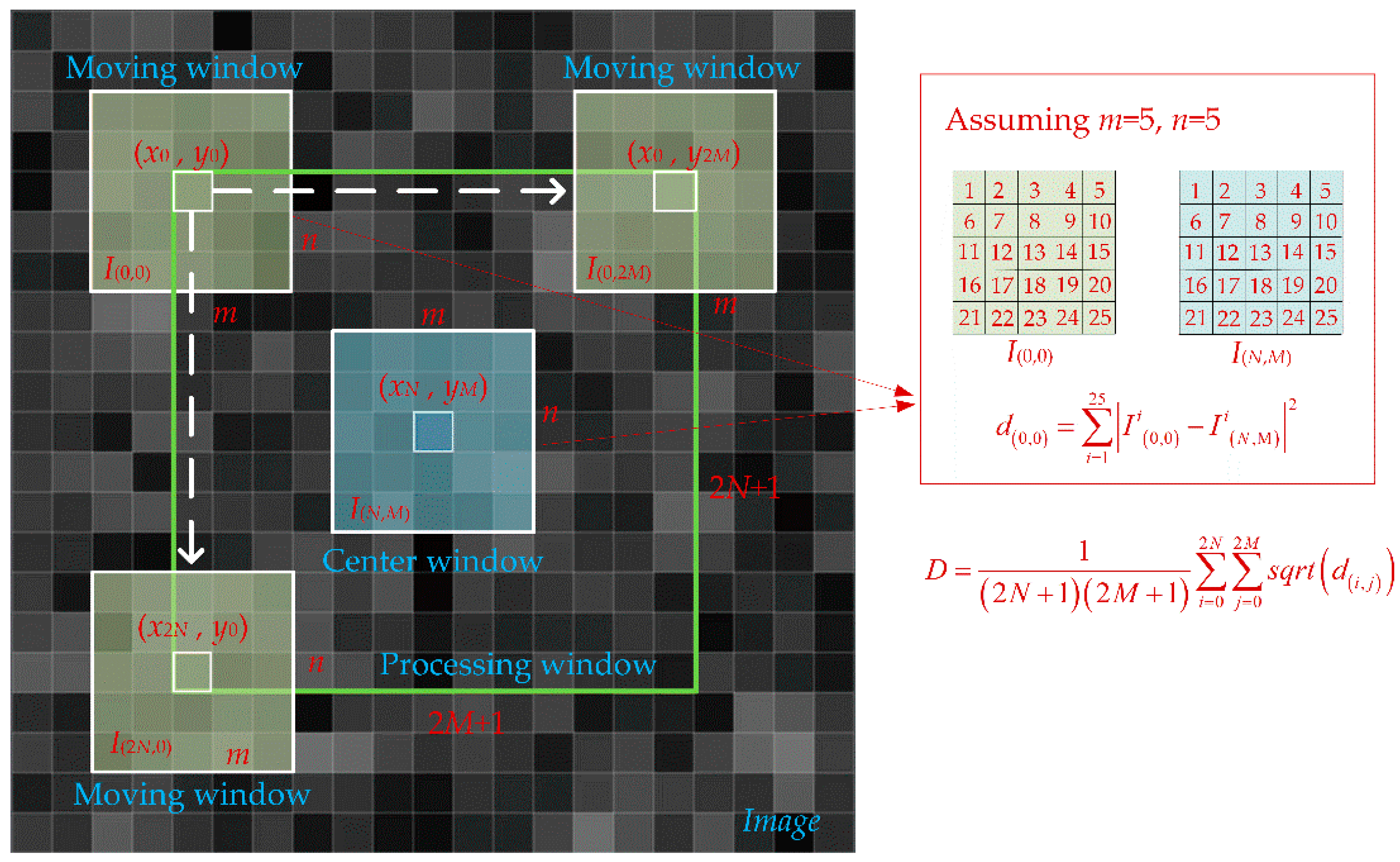
To further describe the degree of similarity between a given pixel relative to its neighbors, the pairwise Euclidean distances between the pixel and every other pixel in the neighborhood is calculated separately according to Equation (16). The average value of the sum of all pairwise Euclidean distances of all the pixels in the region may then be taken and used to define a new edge detection operator, which serves as the approximate description of the pixel point within the surrounding neighborhood. The calculation for the Euclidean distance edge detection operator is shown in Figure 1, and the specific steps are as follows:
Step 1: As shown in Figure 1, create a processing window (the window size is (2M + 1) × (2N + 1)) at the image pending calculation point (xN, yM).
Step 2: In the processing window, create a center window (the window size is m × n and m × n is smaller than (2M + 1) × (2N + 1) at the image pending calculation point (xN, yM).
Step 3: In the processing window, create the m × n size of the corresponding moving window centered on the upper left starting pixel (x0, y0).
Step 4: According to Equation (16), calculate the Euclidean distance between the center window and the corresponding moving window.
Step 5: In the processing window, from left to right and from top to bottom, move the corresponding moving windows sequentially by pixels, and refer to Step 4 to calculate the Euclidean distances of the center window and the corresponding moving windows one by one.
Step 6: Calculate the average of the Euclidean distances of all the regions obtained in the processing window (see Equation (17)) and assign it to the image pending calculation point (xN, yM).
Step 7: The calculation of the complete pixel of the entire image is complete (i.e., the edge detection operator has now been computed).
2.3. Weighting Methods
Section 2.2 describes the use of the Euclidean distance between regions as an edge detection operator. In the windowing process, the effect of each pixel in the window on the center point pixel is considered to be equivalent, and that is not, in fact, the case. Since the detection of the edge point depends on its neighbors, the contribution of the point-to-edge detection that is closer to the position of the edge point is greater. Gaussian weighting and non-linear weighting can be applied to weight each point in the window.
2.3.1. Gaussian Weighting
The Gaussian weight function is defined as follows:
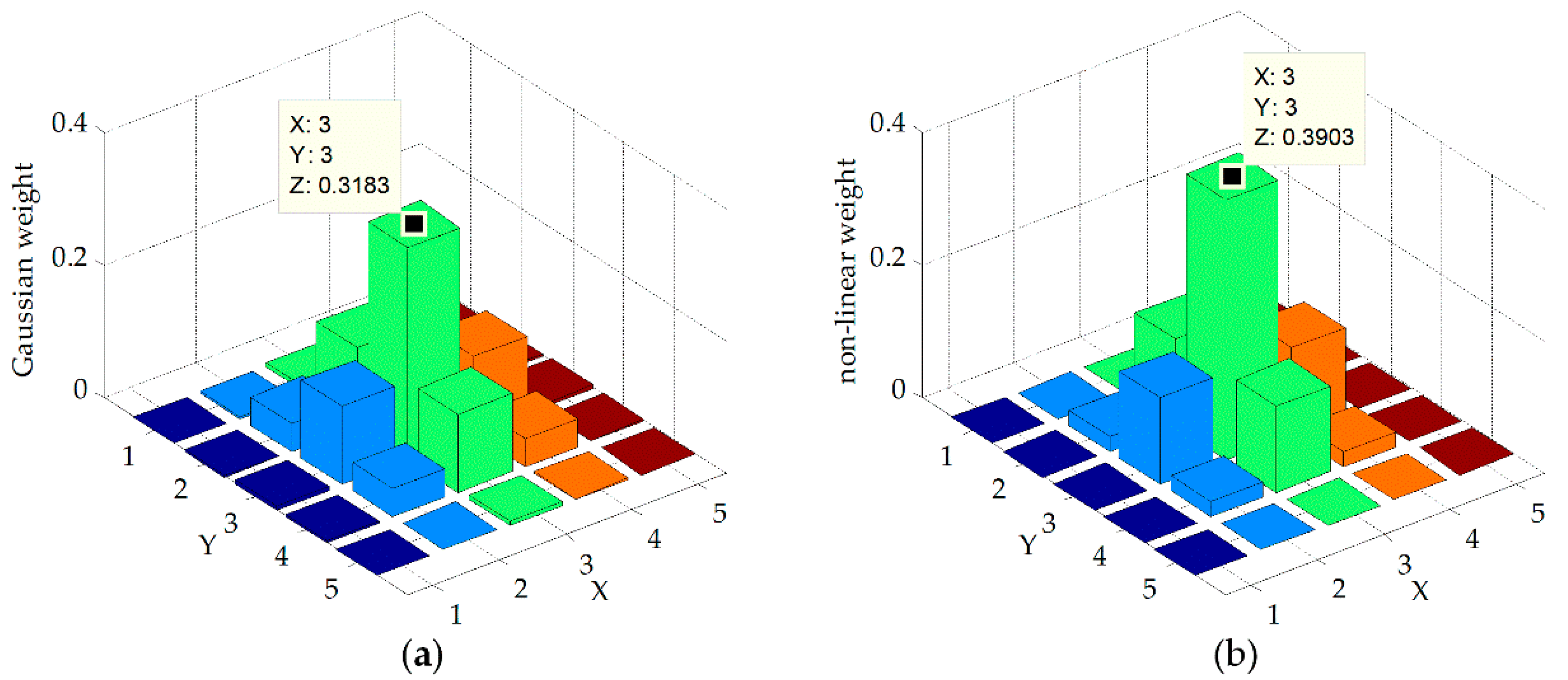
where d is the weighted position distance from the center, h controls the exponential function decay speed, and N plays a normalizing role. Taking a 5 × 5 window as an example, the Gaussian weights of the points in the window are as shown in Figure 2a.
2.3.2. Non-Linear Weighting
The non-linear weight function is defined as follows:
where
where m and n denote the size of window. Taking a 5 × 5 window as an example, the non-linear weights of the points in the window are as shown in Figure 2b.
From Figure 2, it can be seen that both the Gaussian weighting method and the non-linear weighting method yield higher weights to the regions closest to the center point. Taking a 5 × 5 window as an example, the non-linear weighted center point weight is 0.3903, which is greater than the Gaussian weighted center point weight (0.3183). However, in the farther window regions, the Gaussian weight is slightly higher than the non-linear weight.
We can apply two weighting methods to calculate the Euclidean distance edge detection operator. In Step 6 of Euclidean distance edge detection operator calculation, the Euclidean distances from different center points (Calculated according to Equation (16)) contribute different computational weights to the edge detection operators. The closer to the center point, the greater the contribution to the Euclidean distance edge detection operator calculation. Applying Gaussian weights and non-linear weights, Equations (16) and (17) can be updated as follows:
where w(i,j) denotes the weight at the point (i, j) in the processing window using either the Gaussian weighting method or non-linear weighting.
2.4. Method and Processes
The method of WEDAD still uses PDE of SRAD; the main difference compared with SRAD lies in the improvement of the edge detection operator. The WEDAD method uses the Euclidean distance to measure the similarity between pixels, and then achieves an anisotropic diffusion edge detection operator. The novel edge detection operator can be described as:
where x and y are the current pixel position, and Dx,y is the Regional Euclidean distance calculated according to Equations (21) and (22) at position of (x, y) in the SAR image.
The diffusion threshold Tx,y can be obtained as follows:
The diffusion function is:
The essence of the anisotropic diffusion algorithm is to solve partial differential equations. The solving method employed here is the Jacobi iterative algorithm [18], where Δt and Δh are small enough time steps and space steps, respectively. The discrete coordinates of time and space are thus denoted as follows:
This method is applied as follows:
Step 1: Calculate the value of the edge detection operator f of the image pixel-by-pixel according to Equation (21), Equation (22), and Equation (23);
Step 2: Calculate the anisotropic diffusion threshold T according to Equation (24);
Step 3: Then calculate the diffusion coefficient c(f) of image pixels one-by-one according to Equation (25);
Step 4: Next calculate the divergence of {f} c(fx,y) I(x, y; t) in the PDE (Equation (2)), the formula is as follows:
2.5. Evaluation Methods
To evaluate the effect of speckle suppression, the following evaluation indices were used in the experiment.
1. Equivalent Number of Looks (ENL) [28,29]. ENL reflects the degree of speckle suppression, and the formula is as follows:
where E and var are the mean and the variance, respectively, of the image homogeneous area after speckle suppression. A larger ENL indicates that the noise suppression effect is better.
2. Radiate resolution (RS) [30] is a measure of the grayscale resolution capability of SAR systems. It quantitatively represents the ability of an SAR system to distinguish target backscatter coefficients. A smaller RS indicates that the noise suppression effect is better, and the formula for RS is as follows:
3. In a homogeneous region, the ratio of the standard deviation of the image to the mean value is an accurate measure of the intensity of speckle noise. When this value, called the speckle noise index (SNI) [31], is smaller, it indicates that the noise suppression effect is better. SNI can be expressed by the formula:
4. Normalized Mean (NM) [2] is the ratio of the filtered mean value of a region to the average value of the same region before filtering. The formula for NM is as follows:
where EAF and EBF denote the average value after and before filtering in the same region, respectively. NM is a useful criterion for evaluating whether or not a filter provides an unbiased estimate. The closer the normalized mean is to 1, the closer it is to an unbiased estimate, which means that the original information is well-preserved.
5. The edge keeping index (EKI) [29] is used to measure the ability of the speckle suppression method to preserve the edges of the image. The formula is as follows:
where EGVAF and EGVBF denote the gradient value of edge region after and before filtering in the same region, respectively. The closer the edge keeping index is to 1, the better the original information has been preserved.
3. Results and Discussion
3.1. Experiment on an Image with Added Speckle Noise
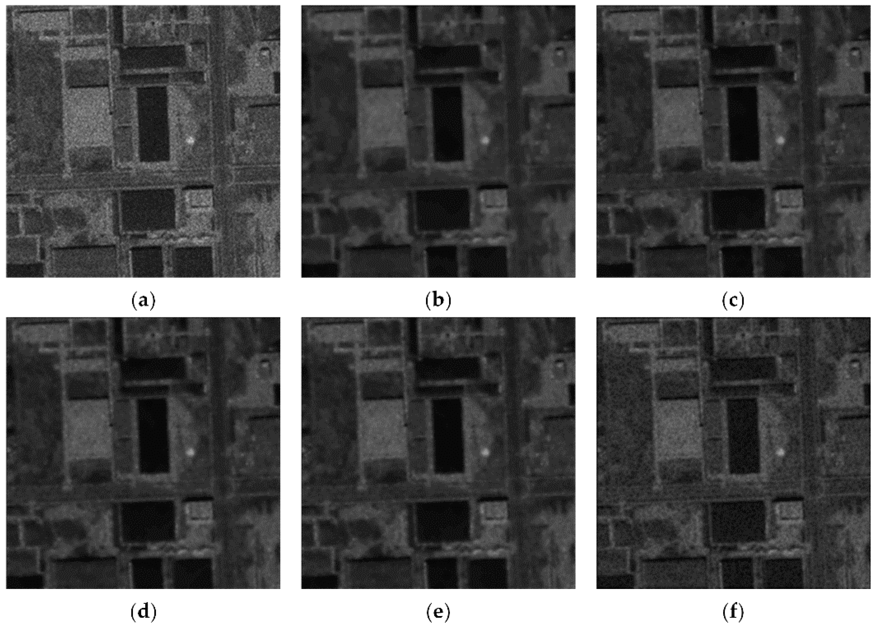
To verify the reliability and validity of the proposed algorithm, multiplicative noise was first added to an original optical image (Figure 3), and each de-noising method based on anisotropic diffusion was applied. The de-noising algorithms were: SRAD, DPAD, AWAD, IEAD, and WEDAD, respectively. In the de-noising processing, the time step was 0.1, and the number of iterations was 50 [22]. The diffusion coefficient in the SRAD model was Equation (3), where f0 = 1, and c = 1/6. In the DPAD method, the sliding window size was 5 × 5, and the noise variation coefficient estimation used an averaging estimation operator [20]. In the AWAD method, the sizes of the selected windows were 3 × 3, 5 × 3 and 3 × 5, respectively, depending on the size of the direction gradient. In the IEAD method, the window size was 5 × 5. In the WEDAD method, the window size of the Euclidean distance edge detection operator calculation was 5 × 5, and Gaussian weighting with 5 × 5 window size was used. Finally, the adjustment coefficient k was 1.0. The experimental results are shown in Figure 4.
From the experimental results, it can be seen that the image filtered by SRAD in Figure 4b has a smoother effect; however, the de-noising image becomes relatively blurry. This is because the instantaneous coefficient of variation in the algorithm is easily interfered with by strong noise, and this affects the accuracy of edge detection. Compared with the SRAD algorithm, the DPAD algorithm improves the noise variation coefficient estimation method, and is also effective at improving the edge maintenance capability, as shown in Figure 4c. The AWAD algorithm adaptively controls the size and direction of the window. The IEAD algorithm uses image entropy to invert the homogenous area and the heterogeneous area. Both of them can improve the edge detection ability, and can obtain a relatively high edge retention during the de-noising process, as shown in Figure 4d,e. The WEDAD algorithm uses weighted Euclidean distance values to reflect the pixel differences and adaptively completes the edge detection, obtaining better edge detection results. The visual effect of this method is the best of those tested, as shown in Figure 4f.
To better demonstrate the capabilities of the algorithm proposed in this paper, we used five objective evaluation criteria (see Section 2.5) to reveal the advantages of the WEDAD algorithm. Table 1 shows the objective evaluation values of each de-noising algorithm for noisy images.
From the objective evaluation criteria shown in Table 1, it can be demonstrated that the WEDAD method shows better performance on five evaluation criteria. The value of ENL of the selected homogeneous area using the WEDAD was 16.403, which is 2.39 times greater than the ENL with no de-noising method, and it is much higher than the value of ENL of the same homogeneous area using the other four algorithms. The WEDAD method also has a lower RS (0.958 dB) and SNI (0.247) than the other four algorithms. Therefore, combining the above three objective evaluation criteria (ENL, RS, and SNI), it can be concluded that the WEDAD method has a significantly better effect on speckle suppression than the other four algorithms. For the other two objective evaluation criteria (NM and EKI), the WEDAD also exhibited higher values, which further indicates that it can better preserve edge information than the other four algorithms. Finally, when comparing the value of ENL with no de-noising method, all five methods have a higher value, which clearly shows that all of these methods can effectively suppress speckle to some degree. Among them, the SRAD method has the second largest ENL, which indicates it can better reduce speckle than DPAP, AWAD, and IEAD. However, the EKI using SRAD is lowest, and therefore the edge retention performance of SRAD is the worst. There is no significant difference in the speckle suppression capabilities of DPAD, AWAD, and IEAD. In these three methods, IEAD can better reduce speckle, and AWAD can better keep edge information.
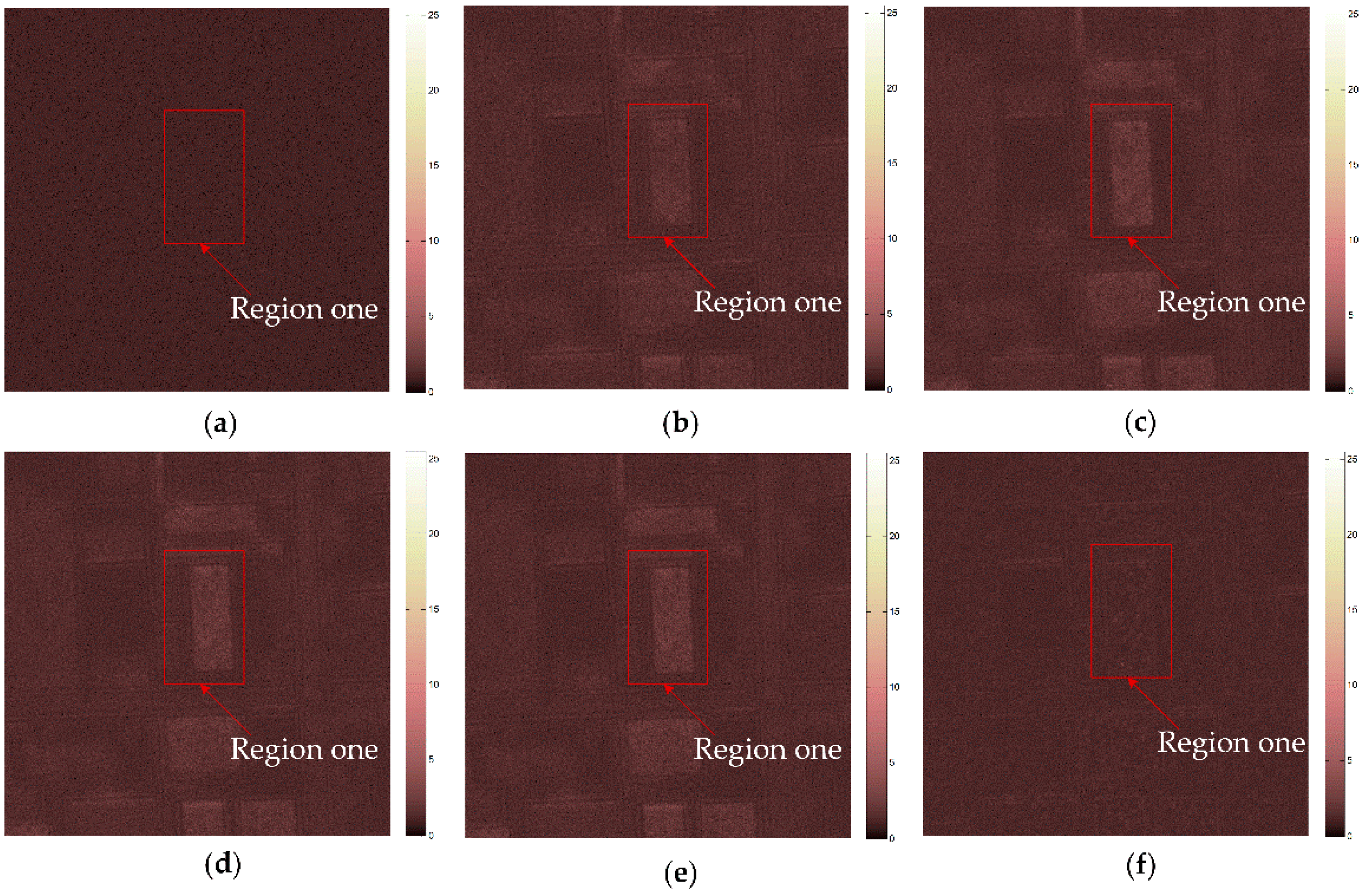
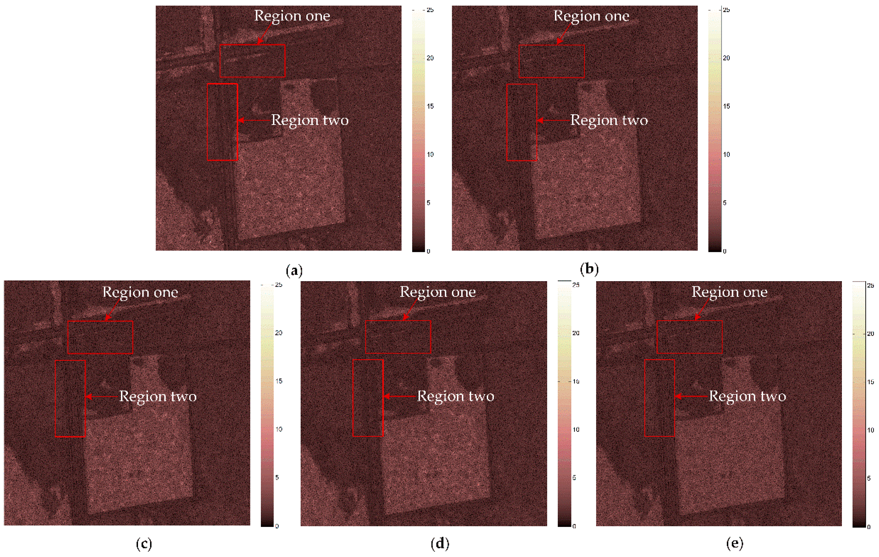
To further demonstrate the performance capabilities of each method, we obtained the ratio images, as mentioned in [28], as the pointwise ratio between the original SAR image and de-noised SAR images. Given a perfect de-noising, the ratio image should contain only speckle [25,28]. However, geometric structures and details correlated to the original image were found, indicating that not only noise but also some information of interest is removed. To better show the difference in the effectiveness of each algorithm, we enhanced the true ratio image by 10 times (as is shown in Figure 5).
It can be seen in Figure 5 that the 10× magnified ratio images generated by the above five speckle suppression methods all include geometric structures or details correlated to the original image, which indicates that all of these de-noising methods destroy the original edge information of the image to some degree. In fact, edge retention and speckle removing are effectively opposite processes. At present, there is no speckle suppression method that completely maintains edge information. However, the effect of preserving the edge was not the same across all methods. Taking the red box region 1 in the image as an example, we may compare Figure 5a (an ideal ratio image) with Figure 5f, which used WEDAD, and has very weak geometric structures and details in spite of the high magnification. Conversely, Figure 5b–e all exhibit strong geometric structures and details compared to both Figure 5a,f. These results further suggest that WEDAD has a better de-noising effect than the other four methods.
3.2. Experiment on Actual SAR Images
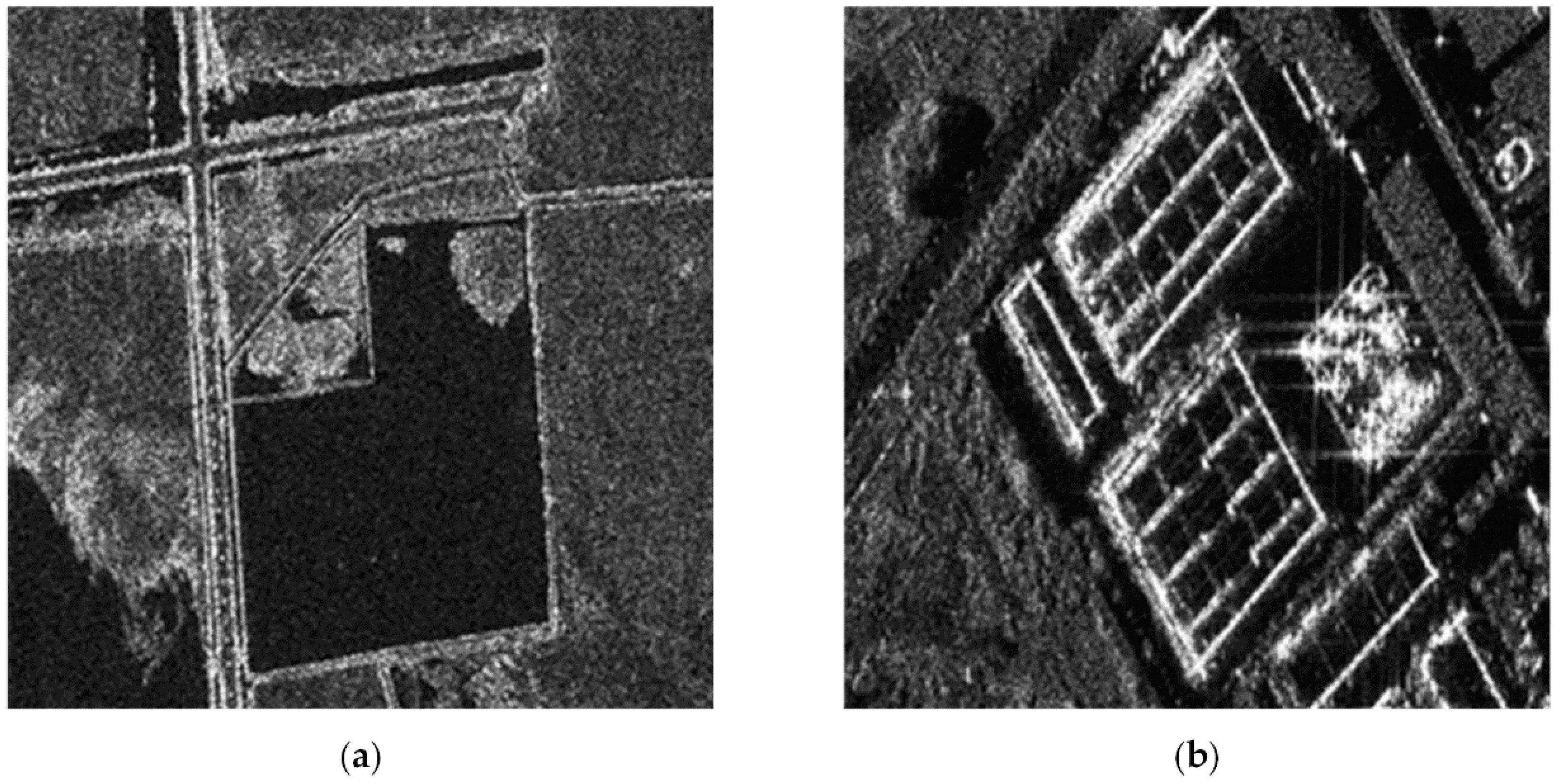
In addition to the independent validity assessment described above, we also tested the proposed algorithm in actual SAR image de-noising processing. GF-3 and YG-29 images were selected, as is shown in Figure 6. Figure 7 shows the resulting de-noised GF-3 images using different noise suppression algorithms. The partial enlargements from Figure 7 is shown in Figure 8. Ratio images generated by different de-noised methods for the GF-3 SAR images are shown in Figure 9 and Figure 10. Figure 11 shows the resulting de-noised YG-29 images using different noise suppression algorithms. The partial enlargements from Figure 11 is shown in Figure 12. Ratio images generated by different de-noised methods for the YG-29 SAR images are shown in Figure 13. Table 2 and Table 3 show the objective evaluation values of each de-noising algorithm for noisy images. The relevant parameter settings of each algorithm are consistent with Section 3.1.
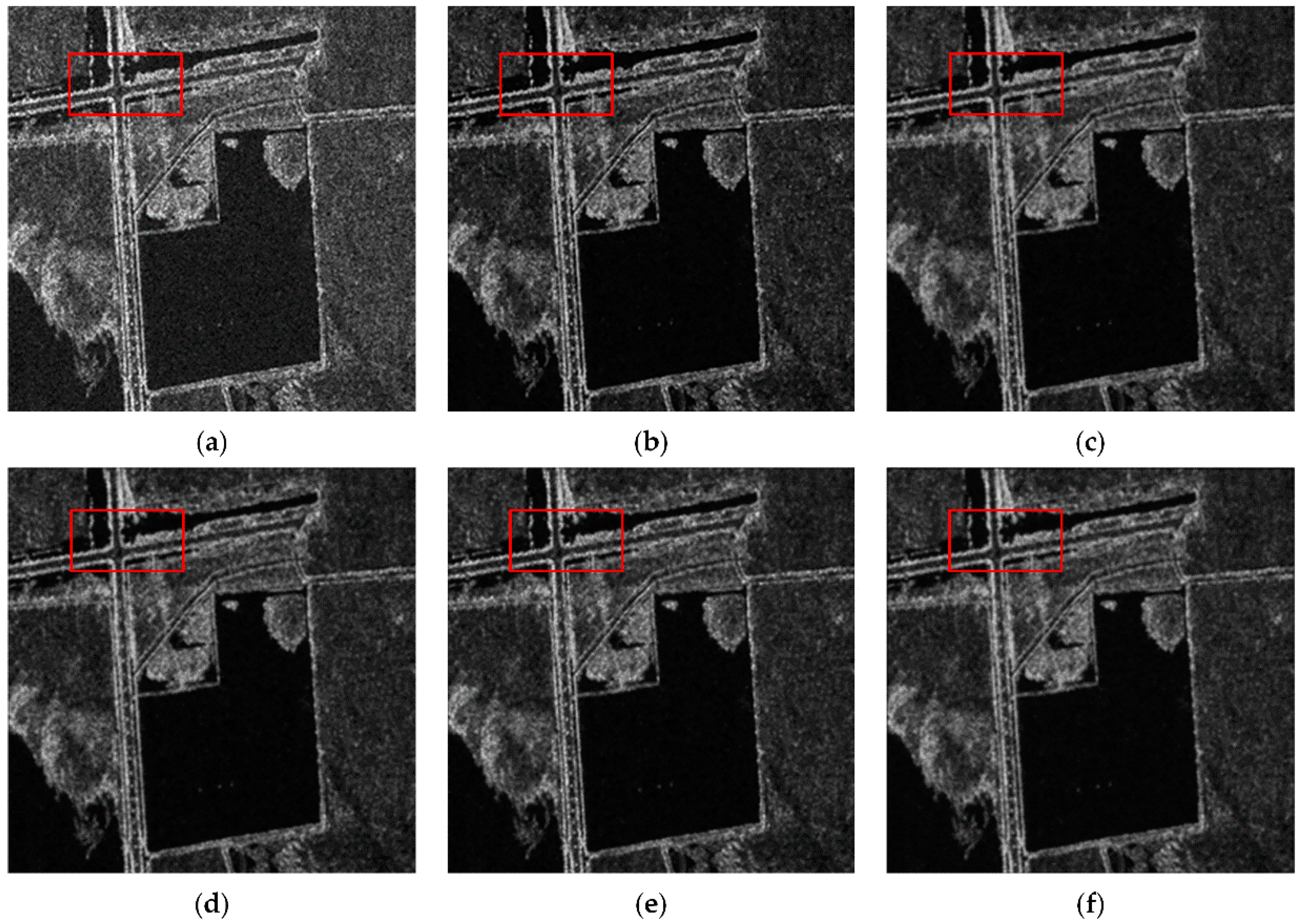
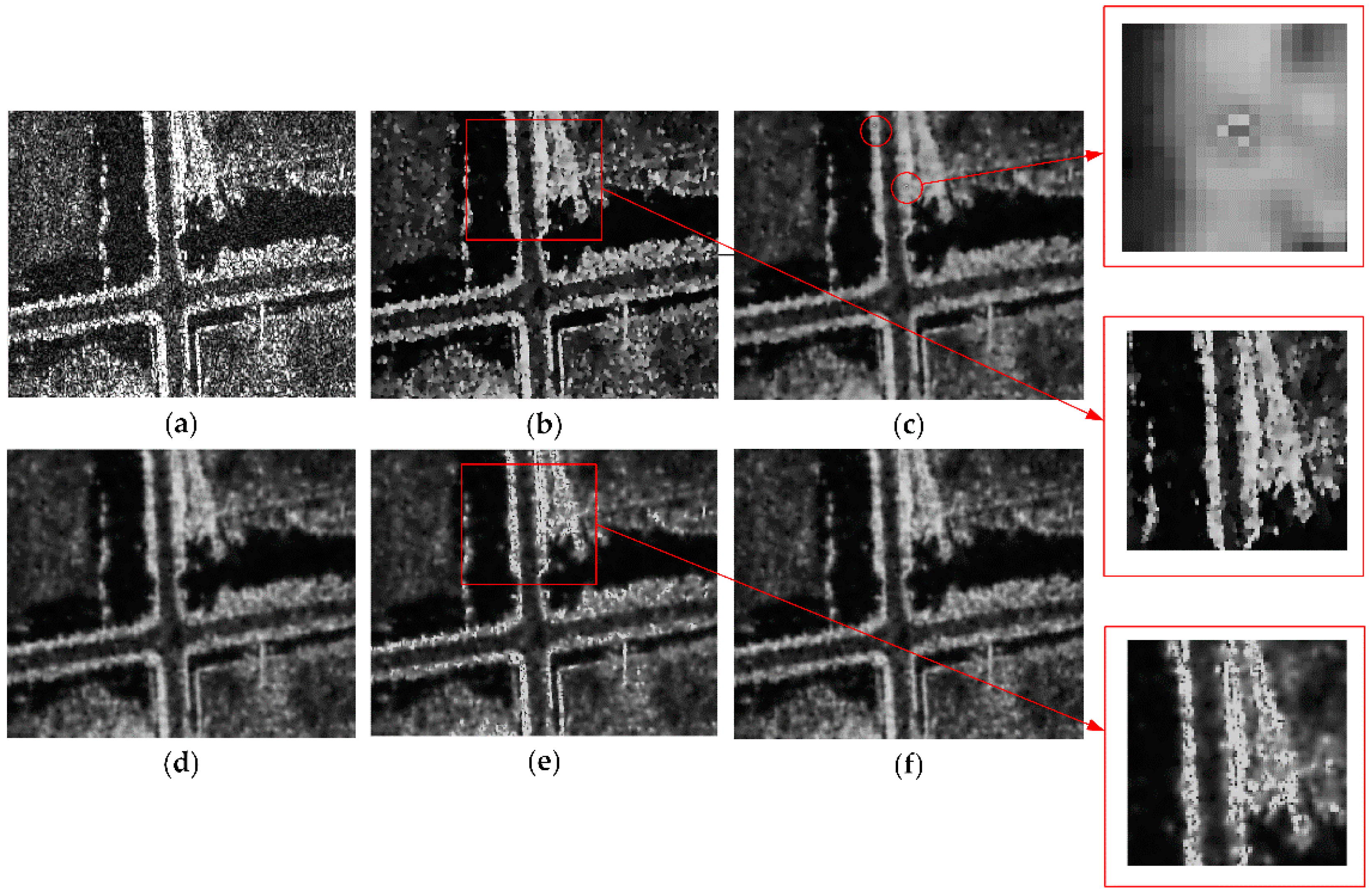
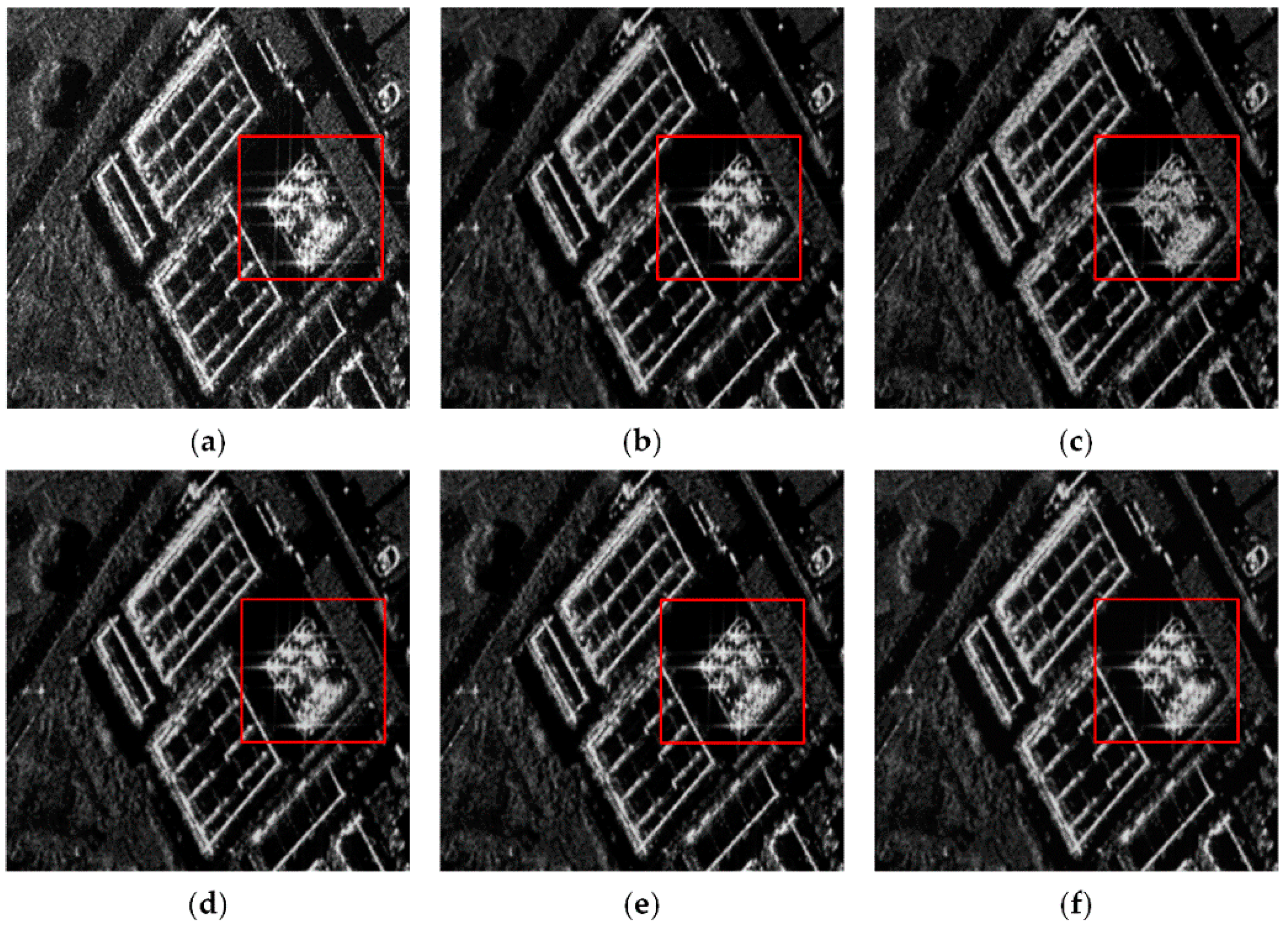
It can be seen in Figure 7 that speckle noise has been smoothed out to varying degrees. To better demonstrate the effect of each de-noised speckle method on a GF-3 image, the red box in Figure 7 was enlarged (Figure 8). Figure 8b uses the SRAD algorithm, and further enlarges the red rectangle. It can be seen that SRAD images are relatively blurry, and that intensity information is incoherent. The overall result of DPAD filtering is better. However, there remain some areas that have not been completely smoothed (see Figure 8c red circle box enlargement). From the further enlarged view of the red rectangular box in Figure 8e, it can be seen that some of the brighter points remained as a result of the IEAD de-noising method. Visually, the AWAD and WEDAD filtering results are relatively good, with WEDAD filtering being the best.
From the objective evaluation criteria shown in Table 2, it can be seen that the algorithm proposed in this paper generally performs better than the other four algorithms. The ENL of the de-noised GF-3 image using WEDAD was 30.405, which is 8.37 times greater when compared with no de-noising method. The ENL of SRAD, IEAD, and AWAD are relatively lower than DPAD and WEDAD, which suggests that WEDAD and DPAD have respectively better speckle reduction effects. From the result of RS and SNI, the same conclusion was made. From the result of NM and EKI, SRAD has the highest NM and a lower EKI, which means that SRAD exhibits better information retention overall, but poor preservation of local edge details. This results from the incoherent intensity information. The result of EKI using IEAD was the lowest, which suggests that this method has a relatively poor performance with respect to edge preservation. This is consistent with Figure 8e. WEDAD has the highest value of EKI and the second highest value of NM (approaching the maximum), which is illustrative of a better edge preservation performance. Overall, WEDAD exhibited the best relative performance for both edge preservation and speckle reduction.
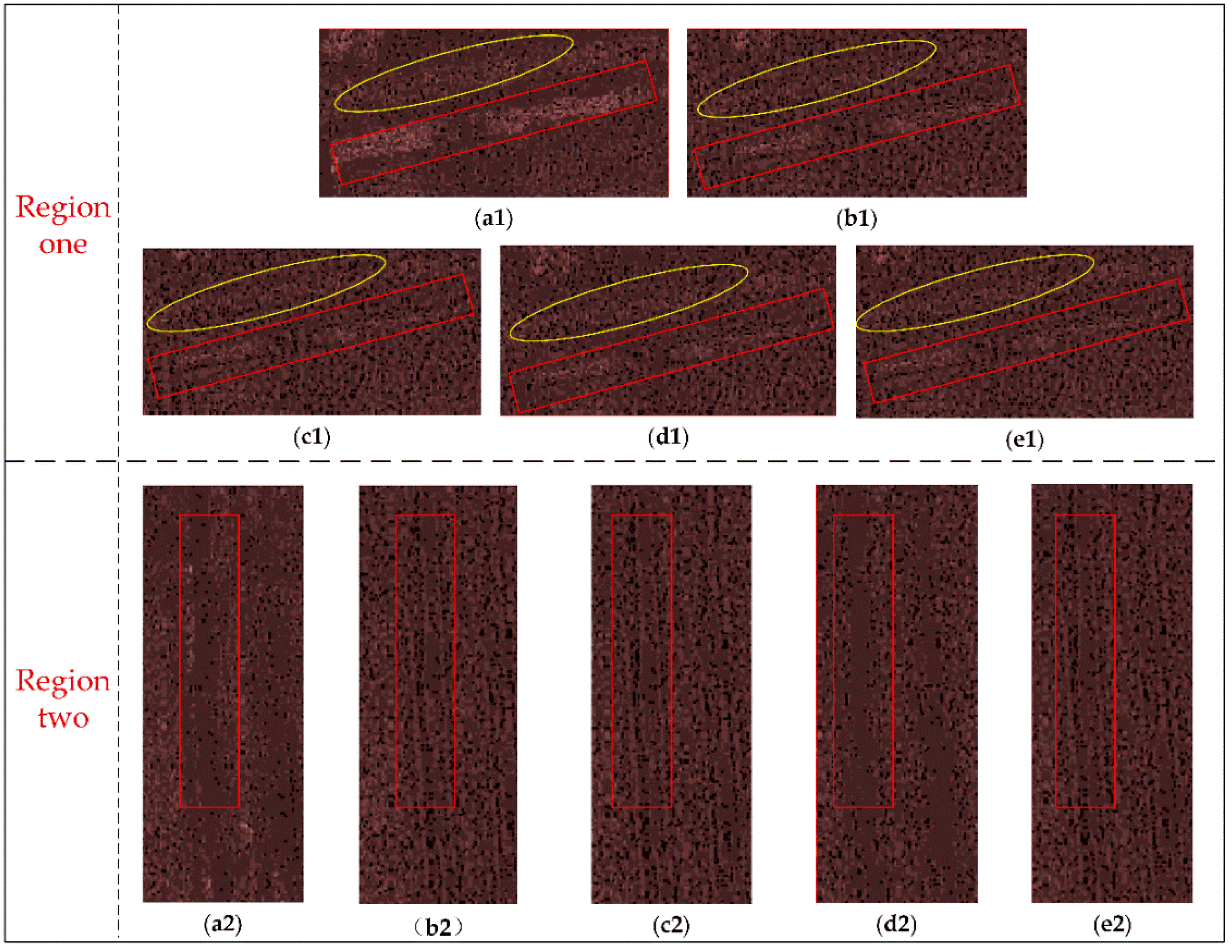
Due to the ratio images in Figure 9 being magnified 10 times, we can see details with relative clarity. In fact, the difference between these images is much smaller than those shown in Figure 9, and they are difficult to visually distinguish. In the absence of true ratio images, we can only compare the horizontal differences between the algorithms. We can see that Figure 9e has relatively darker and more uniform appearance than Figure 9a–d, which suggests that WEDAD has the smallest ratio value, and thereby has the best edge preservation performance. To better show the difference in the details, we further magnified the two red rectangular window regions in Figure 9 (see Figure 10). From the red rectangle and yellow oval box of region one in Figure 10, we can see that SRAD and DPAD remove the most textural information, and that WEDAD removes the least. From the red rectangle box of region two in Figure 10, we can see that SRAD and IEAD remove the most texture information, and that WEDAD still removes the least. The above ratio images also demonstrate the better performance of WEDAD.
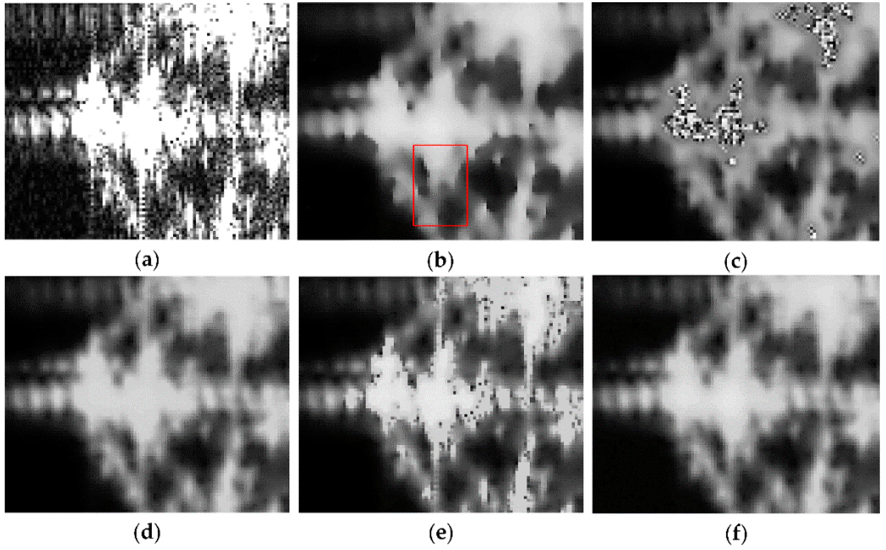
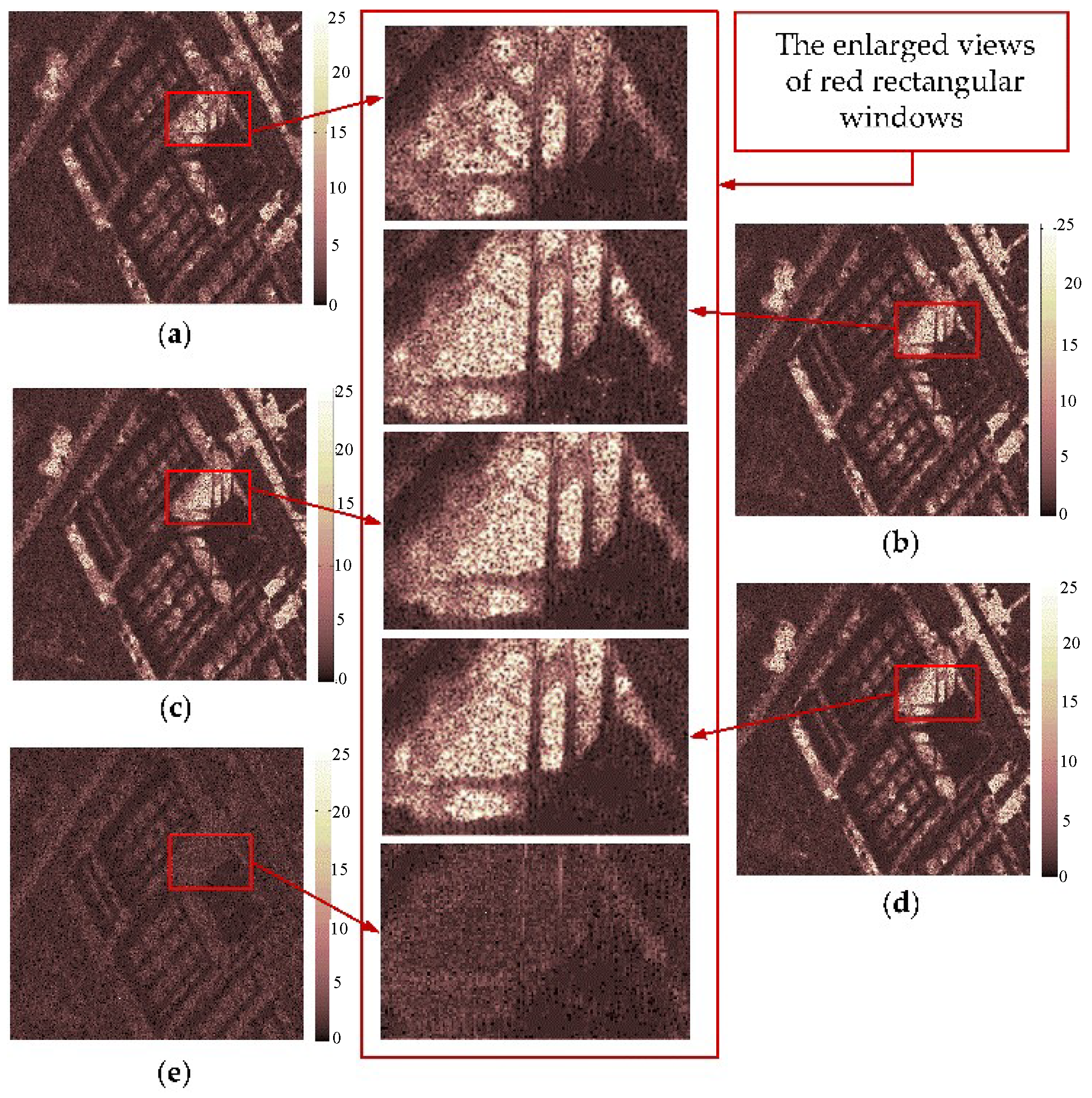
A holistic review of Figure 11 reveals that all five of these algorithms can remove speckle to some extent. To compare the differences in detail processing of each algorithm, a cluster of strong points in the red rectangular box in Figure 11 was enlarged for display (Figure 12). The de-noising results shown in Figure 12 for this area differ among the methods employed. The SRAD method continues to blur the edge information in the red box area of Figure 12b. Both the DPAD method and IEAD method have poor inhibition of the strong points (see Figure 12c,e). The AWAD method and the WEDAD method have better edge preservation performance of these strong points. Figure 12d is darker than Figure 12f. Pixel brightness reflects retention of intensity information. Therefore, WEDAD retains stronger intensity information than AWAD. In summary, WEDAD has better de-noising and edge preservation performance.
From Table 3, WEDAD has the highest ENL, the lowest RS and SNI, which means that WEDAD has a better de-noising performance. The NM value of WEDAD is also optimal. In terms of EKI, DPAD has the best performance. However, the ENL of DPAD is the lowest, which means that DPAD shows better preservation of the local edge details, but poor performance in speckle reduction. The EKI of AWAD, IEAD, and WEDAD are similar and close to the optimal value. The ENL of AWAD and IEAD are obviously lower than WEDAD. From these objective evaluation criteria, WEDAD has better de-noising and edge preservation performance for the YG-29 SAR image.
Figure 13 further compares the performance of each algorithm. Figure 13a–d all have some relatively bright areas, which illustrates that these areas have higher ratio values. Referring to the ideal ratio image (see Figure 5a), this is obviously not a good de-noising effect. The WEDAD method can obtain relatively dark ratio images (see Figure 13e), which demonstrates the better de-noising performance compared to the other algorithms. Additionally, it can be seen from the partially-enlarged view of the rectangular window in Figure 13, that at the strong points, in addition to the WEDAD method, the ratio images obtained by other methods have preserved some edge information.
By de-noising the actual images, the results show that the WEDAD has better speckle suppression and edge preserving performance. It therefore appears to be a more effective speckle-suppression algorithm.
3.3. The Influence of Weighting Methods on Euclidean Distance Anisotropic Diffusion (EDAD)
The Gaussian weighting method was used in the above experiments. We then specifically analyzed the effects of non-linear weights and Gaussian weights. No weighting method, the non-linear weighting method, and the Gaussian weighting method were used to reduce speckle in the added-noise image, and GF-3 and YG-29 SAR images. The relevant parameter settings of the WEDAD algorithm are consistent with Section 3.1. Table 4 shows the objective evaluation (ENL and EKI) of different weighting methods for the EDAD method.
Five homogeneous areas were selected to calculate ENL. From the results of using different weighting methods on the added-noise image, we found that the ENL without using any weighting method had the most optimal values; however, its EKI was the lowest. When using the non-linear weighting and the Gaussian weighting methods, the EKI increased from 0.748 to 0.782 and 0.780, respectively. In the GF-3 SAR image de-noising process using weighting, we found that the ENL using any weighting method was higher than the method with no weighting in all five homogeneous areas. The values of EKI using the two weighting methods were not much different, and both of them were higher than the method using no weighting. When processing of image YG-29 using the different weighting methods, the same conclusion as processing the GF-3 SAR image was obtained for the value of ENL, which demonstrates that both the Gaussian weighting and non-linear weighting methods have higher ENL than the method with no weighting. In terms of EKI, these three weighting methods (including no weighting) have the same value, which means the same edge preservation performance.
Based on the above experiments, it can be seen overall that the method proposed in this paper after the weight function used can generally improve the quality of the speckle filtering. There is no significant difference between the non-linear weights and Gaussian weights.
3.4. The Influence of Adjustment Coefficient on WEDAD
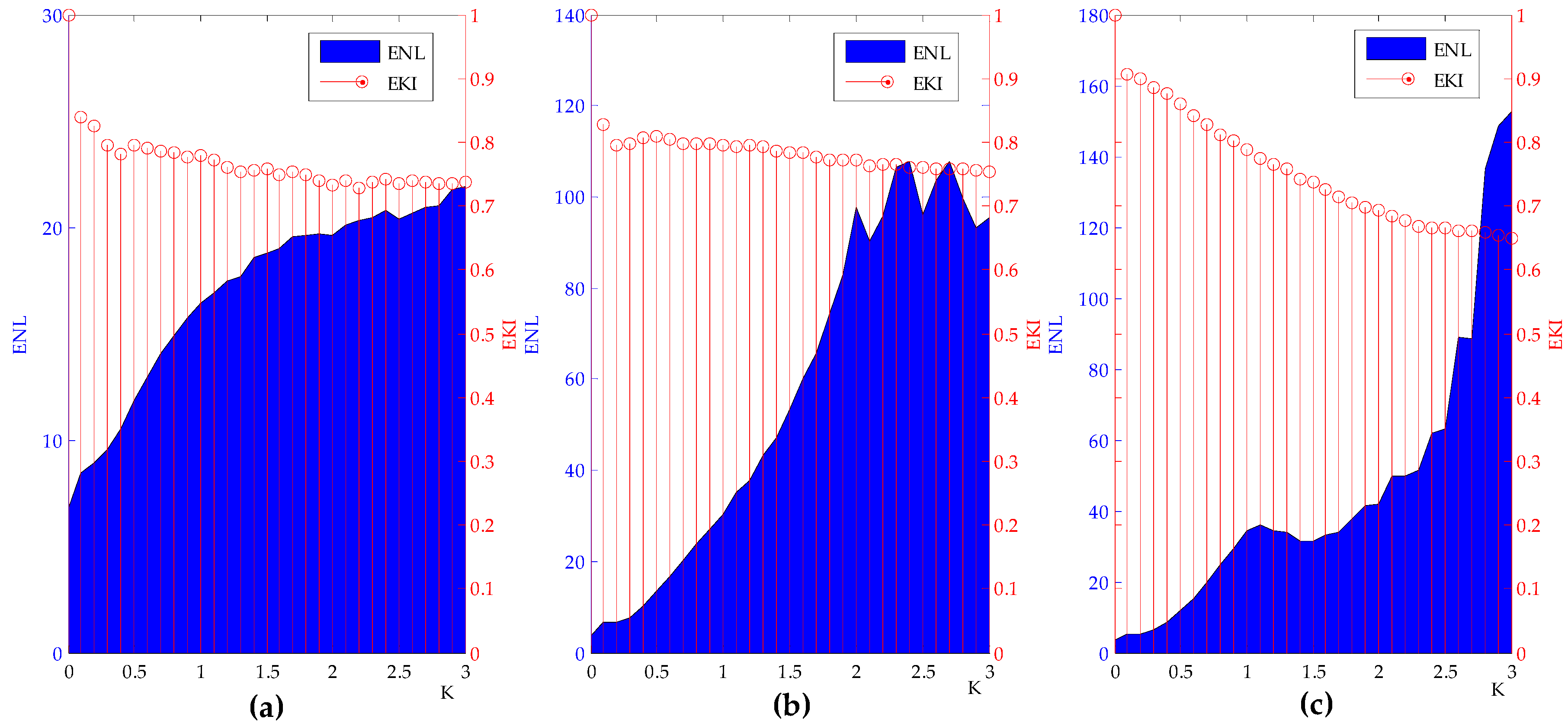
Different time steps and space steps were set, and the corresponding filtering effect was different. The adjustment coefficient k in Equation (28) can effectively balance the influence of setting the time step and space step to the right side of the equation. To obtain the optimal value of adjustment coefficient k, relevant experiments were performed for the three images shown in Figure 3b and Figure 6. Using the WEDAD method, the relevant parameters were set in accordance with Section 3.1, with a time step of 0.1 and a space step of 1. The value of k ranged from 0 to 3 in steps in 0.1. In addition, the objective evaluation (ENL and EKI) were chosen to evaluate the effect of de-noising using different values of k. Figure 14 shows the results of the influence of adjusting the coefficient on different speckle images.
From Figure 14, it can be seen that different values of k have an obvious effect on all three images. In EKI of the three images, there is a maximum of 1 when k is 0. This is because no filtering is actually performed at this time. When the value of k increases, the overall value of EKI tends to decrease, which means that the edge retention performance decreases. In ENL of the three images, there is a minimum when k is 0. As the value of k increases, the overall value of ENL tends to also increase, which means that the speckle reduction performance increases. Therefore, we can find that the increment of the value of k leads to the two objective evaluations tending to move away from the optimal value. These two opposite results also demonstrated that the inhibition of speckle and edge maintenance are contradictory bodies. In addition, in order to obtain better edge retention and speckle suppression at the same time, it is necessary to reasonably determine the value of k. Based on the better evaluation value relative to the other methods (SRAD, DPAD, AWAD, and IEAD), it is recommended that the value of adjustment coefficient k be approximately 0.9.
4. Conclusions
In this paper, speckle suppression by weighted Euclidean distance anisotropic diffusion was proposed. The presented method used weighted Euclidean distances to avoid the problems of accurately estimating the mean and variance of speckle noise, and overall, it achieved better speckle suppression while preserving important edge information. Noise was first added to the original images, and then GF-3 and YG-29 SAR images were collected for use as experimental data. Several conclusions can be drawn from the results presented herein:
- The proposed method can effectively reduce speckle noise while also better preserving edge information. Compared to other general anisotropic diffusion methods (SRAD, DPAP, AWAD, and IEAD), the values of ENL, RS, SNI, NM, and EKI using WEDAD all exhibited optimal or near-optimal values, and were the best overall.
- The proposed method using the Gaussian weighting or non-linear weighting has a better performance of speckle reduction and edge preservation when compared with the method without any weighting method.
- By setting the adjustment coefficient (the value of adjustment coefficient k is recommended as approximately 0.9), edge retention and speckle reduction can be effectively balanced to achieve relatively good results.
We can conclude that the proposed method has a good noise suppression effect on the added-noise image, GF-3 SAR image, and YG-29 SAR image. However, the algorithm in this paper has not yet been applied to other kinds of coherent images. Our future work will therefore focus on the universality of the algorithm.
Author Contributions
F.G., G.Z., and Q.Z. conceived and designed the experiments; F.G., R.Z., and M.D. performed the experiments; F.G. and K.X. analyzed the data; F.G. wrote the paper.
Acknowledgments
This work was supported by, Key research and development program of Ministry of science and technology (2016YFB0500801), National Natural Science Foundation of China (Grant No. 91538106, Grant No. 41501503, 41601490, Grant No. 41501383), China Postdoctoral Science Foundation (Grant No. 2015M582276), Hubei Provincial Natural Science Foundation of China (Grant No. 2015CFB330), Open Research Fund of State Key Laboratory of Information Engineering in Surveying, Mapping and Remote Sensing (Grant No. 15E02), Open Research Fund of State Key Laboratory of Geo-information Engineering (Grant No. SKLGIE2015-Z-3-1), Fundamental Research Funds for the Central University (Grant No. 2042016kf0163). The authors also thank the anonymous reviews for their constructive comments and suggestions.
Conflicts of Interest
The authors declare no conflict of interest.
References
- Xie, H.; Pierce, L.E.; Ulaby, F.T. SAR speckle reduction using wavelet denoising and Markov random field modeling. IEEE Trans. Geosci. Remote Sens. 2002, 40, 2196–2212. [Google Scholar] [CrossRef]
- Oliver, C.; Quegan, S. Understanding Synthetic Aperture Radar Images; Artech House: Boston, MA, USA, 1998. [Google Scholar]
- Lee, J. Digital Image Enhancement and Noise Filtering by Use of Local Statistics. IEEE Trans. Pattern Anal. Mach. Intell. 1980, PAMI-2, 165–168. [Google Scholar] [CrossRef]
- Kuan, D.T.; Sawchuk, A.A.; Strand, T.C.; Chavel, P. Adaptive Noise Smoothing Filter for Images with Signal-Dependent Noise. IEEE Trans. Pattern Anal. Mach. Intell. 1985, PAMI-7, 165–177. [Google Scholar] [CrossRef]
- Frost, V.S.; Stiles, J.A.; Shanmugan, K.S.; Holtzman, J.C. A Model for Radar Images and Its Application to Adaptive Digital Filtering of Multiplicative Noise. IEEE Trans. Pattern Anal. Mach. Intell. 1982, PAMI-4, 157–166. [Google Scholar] [CrossRef]
- Lee, J. Digital Image Smoothing and the Sigma Filter. Comput. Vis. Graphics Image Process. 1983, 24, 255–269. [Google Scholar] [CrossRef]
- Lee, J. Refined Filtering of Image Noise Using Local Statistics. Comput. Vis. Graphics Image Process. 1981, 15, 380–389. [Google Scholar] [CrossRef]
- Lee, J.S.; Wen, J.H.; Ainsworth, T.L.; Chen, K.S.; Chen, A.J. Improved Sigma Filter for Speckle Filtering of SAR Imagery. IEEE Trans. Geosci. Remote Sens. 2009, 47, 202–213. [Google Scholar]
- Lopes, A.; Touzi, R.; Nezry, E. Adaptive Speckle Filters and Scene Heterogeneity. IEEE Trans. Geosci. Remote Sens. 1990, 28, 992–1000. [Google Scholar] [CrossRef]
- Touzi, R. A review of speckle filtering in the context of estimation theory. IEEE Trans. Geosci. Remote Sens. 2002, 40, 2392–2404. [Google Scholar] [CrossRef]
- Wang, B.H.; Zhao, C.Y.; Liu, Y.Y. An improved SAR interferogram denoising method based on principal component analysis and the Goldstein filter. Remote Sens. Lett. 2018, 9, 81–90. [Google Scholar] [CrossRef]
- Achim, A.; Tsakalides, P.; Bezerianos, A. SAR image denoising via Bayesian wavelet shrinkage based on heavy-tailed modeling. IEEE Trans. Geosci. Remote Sens. 2003, 41, 1773–1784. [Google Scholar] [CrossRef]
- Ranjani, J.J.; Thiruvengadam, S. Dual-tree complex wavelet transform based SAR despeckling using interscale dependence. IEEE Trans. Geosci. Remote Sens. 2010, 48, 2723–2731. [Google Scholar] [CrossRef]
- Gleich, D.; Kseneman, M.; Datcu, M. Despeckling of TerraSAR-X data using second-generation wavelets. IEEE Trans. Geosci. Remote Sens. Lett. 2010, 7, 68–72. [Google Scholar] [CrossRef]
- Hou, B.; Zhang, X.; Bu, X.; Feng, H. SAR image despeckling based on nonsubsampled shearlet transform. IEEE J. Sel. Top. Appl. Earth Obs. Remote Sens. 2012, 5, 809–823. [Google Scholar] [CrossRef]
- Liu, S.; Shi, M.; Hu, S.; Xiao, Y. Synthetic aperture radar image de-noising based on Shearlet transform using the context-based model. Phys. Commun. 2014, 13, 221–229. [Google Scholar] [CrossRef]
- Perona, P.; Malik, J. Scale-Space and Edge Detection Using Anisotropic Diffusion. IEEE Trans. Pattern Anal. Mach. Intell. 1990, 12, 629–639. [Google Scholar] [CrossRef]
- Yongjian, Y.; Scott, T.A. Speckle Reducing Anisotropic Diffusion. IEEE Trans. Image Process. 2002, 11, 1260–1270. [Google Scholar] [CrossRef] [PubMed]
- Li, J.C. The Research on Speckle Reduction for Synthetic Aperture Radar Images; National University of Defense Technology: Changsha, China, 2014. [Google Scholar]
- Aja-Fernández, S.; Alberola-López, C. On the estimation of the coefficient of variation for anisotropic diffusion speckle filtering. IEEE Trans. Image Process. 2006, 15, 2694–2701. [Google Scholar] [CrossRef] [PubMed]
- Liu, G.; Zeng, X.; Tian, F.; Li, Z.; Chaibou, K. Speckle reduction by adaptive window anisotropic diffusion. Signal Process. 2009, 89, 2233–2243. [Google Scholar] [CrossRef]
- Li, J.C.; Ma, Z.H.; Peng, Y.X.; Huang, H. Speckle reduction by image entropy anisotropic diffusion. Acta Phys. Sin. 2013, 62, 099501. [Google Scholar]
- Zhang, C.; Wang, T.T.; Sun, D.J. Image edge detection based on the Euclidean distance graph. J. Image Graph. 2013, 18, 176–183. [Google Scholar]
- Dai, M.; Peng, C.; Chan, A.K.; Loguinov, D. Bayesian wavelet shrinkage with edge detection for SAR image despeckling. IEEE Trans. Geosci. Remote Sens. 2004, 42, 1642–1648. [Google Scholar]
- Liu, S.; Hu, Q.; Li, P.F.; Zhao, J. Speckle Suppression Based on Sparse Representation with Non-Local Priors. Remote Sens. 2018, 10, 439. [Google Scholar] [CrossRef]
- Tabassum, N.; Vaccari, A.; Acton, S. Speckle removal and change preservation by distance-driven anisotropic diffusion of synthetic aperture radar temporal stacks. Digit. Signal Process. 2018, 74, 43–55. [Google Scholar] [CrossRef]
- Qiao, M.; Wang, X.L.; Zou, M.Y. A regularized anisotropic diffusion for speckle reducing. J. Grad. Sch. Chin. Acad. Sci. 2005, 22, 24–29. [Google Scholar]
- Parrilli, S.; Poderico, M.; Angelino, C.V.; Verdoliva, L. A nonlocal SAR image denoising algorithm based on LLMMSE wavelet shrinkage. IEEE Trans. Geosci. Remote Sens. 2012, 50, 606–616. [Google Scholar] [CrossRef]
- Zhu, L.; Han, T.Q.; Shui, P.L.; Wei, J.H.; Gu, M.H. An anisotropic diffusion filtering method for speckle reduction of synthetic aperture radar images. Acta Phys. Sin. 2014, 63, 179502. [Google Scholar]
- Wei, Z.Q. Synthetic Aperture Radar Satellite; Science Press: Beijing, China, 2001. [Google Scholar]
- Crimmins, T.R. Geometric Filter For Reducing Speckle. Opt. Eng. 1985, 25, 651–654. [Google Scholar]
Figure 1.
Euclidean distance edge detection operator calculation.

Figure 2.
Weight histograms of the points in a 5 × 5 window: (a) Gaussian weight (h = 1); (b) non-linear weight.
Figure 2.
Weight histograms of the points in a 5 × 5 window: (a) Gaussian weight (h = 1); (b) non-linear weight.

Figure 3.
The original image and added-noise image: (a) Original image; (b) added-noise image (the mean is 1 and the variance is 0.1).
Figure 3.
The original image and added-noise image: (a) Original image; (b) added-noise image (the mean is 1 and the variance is 0.1).

Figure 4.
The images generated by different de-noising methods: (a) No filtering method; (b) SRAD; (c) DPAD; (d) AWAD; (e) IEAD; (f) WEDAD.
Figure 4.
The images generated by different de-noising methods: (a) No filtering method; (b) SRAD; (c) DPAD; (d) AWAD; (e) IEAD; (f) WEDAD.

Figure 5.
The ratio images generated by different de-noised methods: (a) Ratio image between the original image and noise image in Figure 3; (b) Ratio image by SRAD; (c) Ratio image by DPAD; (d) Ratio image by AWAD; (e) Ratio image by IEAD; (f) Ratio image by WEDAD.
Figure 5.
The ratio images generated by different de-noised methods: (a) Ratio image between the original image and noise image in Figure 3; (b) Ratio image by SRAD; (c) Ratio image by DPAD; (d) Ratio image by AWAD; (e) Ratio image by IEAD; (f) Ratio image by WEDAD.

Figure 6.
The actual synthetic aperture radar (SAR) images: (a) GF-3 image; (b) YG-29 image.

Figure 7.
The GF-3 images using different de-noising methods: (a) No filtering method; (b) SRAD; (c) DPAD; (d) AWAD; (e) IEAD; (f) WEDAD.
Figure 7.
The GF-3 images using different de-noising methods: (a) No filtering method; (b) SRAD; (c) DPAD; (d) AWAD; (e) IEAD; (f) WEDAD.

Figure 8.
The partial enlargement of GF-3 images using different de-noising methods: (a) No filtering method; (b) SRAD; (c) DPAD; (d) AWAD; (e) IEAD; (f) WEDAD.
Figure 8.
The partial enlargement of GF-3 images using different de-noising methods: (a) No filtering method; (b) SRAD; (c) DPAD; (d) AWAD; (e) IEAD; (f) WEDAD.

Figure 9.
The ratio images generated by different de-noised methods for the GF-3 SAR image: (a) Ratio image by SRAD; (b) ratio image by DPAD; (c) ratio image by AWAD; (d) ratio image by IEAD; (e) ratio image by WEDAD.
Figure 9.
The ratio images generated by different de-noised methods for the GF-3 SAR image: (a) Ratio image by SRAD; (b) ratio image by DPAD; (c) ratio image by AWAD; (d) ratio image by IEAD; (e) ratio image by WEDAD.

Figure 10.
The partially enlarged views of ratio images from Figure 9. (a1) partially enlarged view of region one in the ratio image by SRAD. (b1) partially enlarged view of region one in the ratio image by DPAD. (c1) partially enlarged view of region one in the ratio image by AWAD. (d1) partially enlarged view of region one in the ratio image by IEAD. (e1) partially enlarged view of region one in the ratio image by WEDAD. (a2) partially enlarged view of region two in the ratio image by SRAD. (b2) partially enlarged view of region two in the ratio image by DPAD. (c2) partially enlarged view of region two in the ratio image by AWAD. (d2) partially enlarged view of region two in the ratio image by IEAD. (e2) partially enlarged view of region two in the ratio image by WEDAD.

Figure 11.
The YG-29 images using different de-noising methods: (a) No filtering method; (b) SRAD; (c) DPAD; (d) AWAD; (e) IEAD; (f) WEDAD.
Figure 11.
The YG-29 images using different de-noising methods: (a) No filtering method; (b) SRAD; (c) DPAD; (d) AWAD; (e) IEAD; (f) WEDAD.

Figure 12.
The partially enlarged views of YG-29 images using different de-noising methods: (a) No filtering method; (b) SRAD; (c) DPAD; (d) AWAD; (e) IEAD; (f) WEDAD.
Figure 12.
The partially enlarged views of YG-29 images using different de-noising methods: (a) No filtering method; (b) SRAD; (c) DPAD; (d) AWAD; (e) IEAD; (f) WEDAD.

Figure 13.
The ratio images generated by different de-noised methods on YG-29 SAR image: (a) Ratio image by SRAD; (b) ratio image by DPAD; (c) ratio image by AWAD; (d) ratio image by IEAD; (e) ratio image by WEDAD.
Figure 13.
The ratio images generated by different de-noised methods on YG-29 SAR image: (a) Ratio image by SRAD; (b) ratio image by DPAD; (c) ratio image by AWAD; (d) ratio image by IEAD; (e) ratio image by WEDAD.

Figure 14.
The influence of the adjustment coefficient on different speckle images: (a) the influence of the adjustment coefficient on added noise image; (b) the influence of the adjustment coefficient on the GF-3 SAR image; (c) the influence of the adjustment coefficient on the YG-29 SAR image.
Figure 14.
The influence of the adjustment coefficient on different speckle images: (a) the influence of the adjustment coefficient on added noise image; (b) the influence of the adjustment coefficient on the GF-3 SAR image; (c) the influence of the adjustment coefficient on the YG-29 SAR image.


Table 1.
Objective evaluation of different de-noising methods.
| Methods | ENL | RS (dB) | SNI | NM | EKI |
|---|---|---|---|---|---|
| Ideal Value | - | - | - | 1.000 | 1.000 |
| None | 6.859 | 1.405 | 0.382 | - | - |
| SRAD | 12.345 | 1.088 | 0.285 | 0.754 | 0.741 |
| DPAD | 11.718 | 1.113 | 0.292 | 0.753 | 0.732 |
| AWAD | 11.672 | 1.115 | 0.293 | 0.752 | 0.755 |
| IEAD | 11.816 | 1.109 | 0.291 | 0.753 | 0.753 |
| WEDAD | 16.403 | 0.958 | 0.247 | 0.784 | 0.780 |
Table 2.
Objective evaluation of different de-noising methods on GF-3 synthetic aperture radar (SAR) image.
Table 2.
Objective evaluation of different de-noising methods on GF-3 synthetic aperture radar (SAR) image.
| Methods | ENL | RS (dB) | SNI | NM | EKI |
|---|---|---|---|---|---|
| Ideal Value | - | - | - | 1.000 | 1.000 |
| None | 3.631 | 1.832 | 0.525 | - | - |
| SRAD | 17.822 | 0.923 | 0.237 | 0.809 | 0.774 |
| DPAD | 22.498 | 0.831 | 0.211 | 0.806 | 0.788 |
| AWAD | 18.996 | 0.897 | 0.229 | 0.805 | 0.794 |
| IEAD | 18.182 | 0.915 | 0.235 | 0.799 | 0.764 |
| WEDAD | 30.405 | 0.724 | 0.181 | 0.807 | 0.795 |
Table 3.
Objective evaluation of different de-noising methods on the YG-29 SAR Image.
| Methods | ENL | RS (dB) | SNI | NM | EKI |
|---|---|---|---|---|---|
| Ideal Value | - | - | - | 1.000 | 1.000 |
| None | 3.431 | 1.875 | 0.540 | - | - |
| SRAD | 25.026 | 0.791 | 0.200 | 0.783 | 0.762 |
| DPAD | 15.596 | 0.980 | 0.253 | 0.782 | 0.790 |
| AWAD | 22.094 | 0.838 | 0.213 | 0.784 | 0.787 |
| IEAD | 21.526 | 0.848 | 0.216 | 0.775 | 0.788 |
| WEDAD | 34.576 | 0.682 | 0.170 | 0.789 | 0.788 |
Table 4.
Objective evaluation of different weighting methods on the EDAD method.
| Images | Weighted Methods | ENL | EKI | ||||
|---|---|---|---|---|---|---|---|
| Region 1 | Region 2 | Region 3 | Region 4 | Region 5 | |||
| Added Speckle Noise | None | 16.623 | 61.024 | 21.968 | 45.185 | 17.431 | 0.748 |
| Non-linear | 16.049 | 62.981 | 21.649 | 44.6 | 16.451 | 0.782 | |
| Gaussian | 16.403 | 64.239 | 21.687 | 44.406 | 16.643 | 0.780 | |
| GF-3 | None | 15.831 | 31.073 | 21.720 | 30.665 | 24.526 | 0.790 |
| Non-linear | 15.858 | 31.118 | 21.763 | 30.674 | 24.548 | 0.794 | |
| Gaussian | 15.861 | 31.133 | 21.760 | 30.683 | 24.538 | 0.795 | |
| YG-29 | None | 21.471 | 17.576 | 18.213 | 17.638 | 15.407 | 0.788 |
| Non-linear | 21.523 | 17.599 | 18.222 | 17.651 | 15.461 | 0.788 | |
| Gaussian | 21.511 | 17.642 | 18.247 | 17.645 | 15.455 | 0.788 | |
© 2018 by the authors. Licensee MDPI, Basel, Switzerland. This article is an open access article distributed under the terms and conditions of the Creative Commons Attribution (CC BY) license (http://creativecommons.org/licenses/by/4.0/).
Share and Cite
MDPI and ACS Style
Guo, F.; Zhang, G.; Zhang, Q.; Zhao, R.; Deng, M.; Xu, K. Speckle Suppression by Weighted Euclidean Distance Anisotropic Diffusion. Remote Sens. 2018, 10, 722. https://0-doi-org.brum.beds.ac.uk/10.3390/rs10050722
AMA Style
Guo F, Zhang G, Zhang Q, Zhao R, Deng M, Xu K. Speckle Suppression by Weighted Euclidean Distance Anisotropic Diffusion. Remote Sensing. 2018; 10(5):722. https://0-doi-org.brum.beds.ac.uk/10.3390/rs10050722
Chicago/Turabian StyleGuo, Fengcheng, Guo Zhang, Qingjun Zhang, Ruishan Zhao, Mingjun Deng, and Kai Xu. 2018. "Speckle Suppression by Weighted Euclidean Distance Anisotropic Diffusion" Remote Sensing 10, no. 5: 722. https://0-doi-org.brum.beds.ac.uk/10.3390/rs10050722
Note that from the first issue of 2016, this journal uses article numbers instead of page numbers. See further details here.