COMS Visible Channel Calibration Using Moon Observation Data

National Meteorological Satellite Center, Korea Meteorological Administration, 64-18 Guam-gil, Gwanghyewon-myeon, Jincheon-gun 27803, Chungcheongbuk-do, Korea
*
Author to whom correspondence should be addressed.
Remote Sens. 2018, 10(5), 726; https://0-doi-org.brum.beds.ac.uk/10.3390/rs10050726
Submission received: 4 April 2018
/
Revised: 3 May 2018
/
Accepted: 6 May 2018
/
Published: 8 May 2018
(This article belongs to the Section Atmospheric Remote Sensing)
Abstract
:COMS (Communication, Ocean, and Meteorological Satellite) has been in operation since April 2011. The COMS MI (Meteorological Imager) has one visible and four infrared channels. Through the use of the GSICS (Global Space-based Inter-Calibration System), the KMA (Korea Meteorological Administration) has monitored the radiometric performance of the COMS visible channel through its own calibration system and the use of four different earth targets: ocean, desert, water cloud, and DCC (Deep Convective Cloud). To use the invariant target of the Moon, the KMA adopted GIRO (GSICS Implementation of the ROLO (Robotic Lunar Observatory) model), which was released by EUMETSAT. In this study, a total of 146 lunar observation data (Level 1A) with various phase angles obtained between April 2011 and December 2017 are analyzed. A degradation rate of approximately −1.52 ± 0.10% per year occurred using the GIRO method, which was a degradation of approximately 12% over the eight years (from 2011 to 2018) during COMS MI’s operational period. The lunar calibration result was in good agreement with results provided by other calibration methods such as the DCC using the RTM (Radiative Transfer Model), which was approximately −1.43 ± 0.13% per year. Selection of on-Moon pixels provided an uncertainty of approximately 0.01% per year, while that related to the phase angle (Sun-Moon-Satellite) was approximately 0.06% per year.
1. Introduction
The Korean geostationary meteorological satellite, COMS (Communication, Ocean, and Meteorological Satellite), is the first operated by the KMA (Korea Meteorological Administration). It was launched on 27 June 2010 and has been in operation since April 2011. COMS MI (Meteorological Imager) is a multichannel imaging radiometer designed to sense radiant and solar-reflected energy from the environs of the Korean Peninsula as well as neighboring seas and countries; it has one visible and four infrared channels.
Accurate instrument calibration is extremely important when converting a signal observed by an instrument (e.g., digital counts) into a stable and accurate physical quantity, such as spectral radiance. Calibration for infrared channels is accomplished by conducting periodic measurements of an on-board blackbody and deep space. Recently, satellite operators have developed an inter-calibration method using a hyper-spectral sounder (e.g., IASI on the Metop series, AIRS on Aqua, CrIS on Suomi-NPP, and JPSS) on LEO (Low Earth Orbiting) satellites as a reference instrument [1,2] under the framework of the GSICS (Global Space-based Inter-Calibration System, [3]). For visible channel on-board calibration equipment with a highly advanced performance, recent instruments such as MODIS (Moderate Resolution Imaging Spectroradiometer) and VIIRS (Visible Infrared Imaging Radiometer Suite) use a solar diffuser [4,5]. Similarly, COMS MI is equipped with an Albedo Monitor as an on-board radiometric calibration device. However, the calibration system used by the Albedo Monitor of COMS cannot be implemented for monitoring long-term degradation of the visible channel as it has a larger uncertainty than the signal. Therefore, the use of other calibration methods is necessary for long-term monitoring of sensor degradation.
To monitor and analyze visible channel degradation and stability, a variety of post-launch calibration techniques have been developed by the satellite operation community. Vicarious calibration, which uses a not-in-orbit stable object as the calibration reference target, is employed to examine the sensor in-orbit degradation patterns or to provide post-launch calibration coefficients. To reduce the risk of erroneous degradation trending, multiple calibration methods are often used to verify results. In this respect, several vicarious calibration methods, which use different stable targets, have been studied for use with COMS visible channels; KMA has implemented inter-calibration methods for geostationary meteorological imagers within the framework of GSICS, with calibration targets of the DCC (Deep Convective Cloud) and the Moon. Vicarious calibration methods using a radiative transfer simulation have also been developed in collaboration with Seoul National University [6]. These calibration methods use invariant Earth surface targets such as deserts [7], DCC [8,9], Rayleigh scattering, and sun-glint over a clear ocean surface [10,11], and assume that the time-series of stable reference target observations (either direct satellite measurements or ratios of satellite measurements to modeled simulations of the reference) are scattered along a trend that can be used to describe the instrument degradation pattern. However, the performance of reference targets needs to be well understood and characterized to estimate and understand calibration uncertainty; when short-term variations in reference targets are well understood and characterized, they can be removed or simulated to improve calibration accuracy [12].
On the basis of these reference targets, vicarious calibration methods can provide either relative or absolute calibration correction coefficients. The Sonoran Desert is one of the largest deserts in North America and can be observed by both GOES (Geostationary Operational Environmental Satellite)-East and GOES-West satellites. It has long-term stability and can thus be used as a reference target for the development of long-term GOES visible climate data with calibration accuracy traceable to MODIS Collection 6 data at about 3–4% [13]. However, as a result of the impacts of a strong BRDF (Bidirectional Reflectance Distribution Function) effect and occasional climate variations such as ENSO (El Niño–Southern Oscillation) events, it is not an appropriate reference target for use with operational or near real-time data calibration.
The DCC has high reflectance and relatively flat spectra in the visible wavelength range; as such, it can be used as a stable reference target to provide an absolute calibration accuracy of less than 3% for the GEO (Geostationary Satellite) visible channels and that of less than 1% for the LEO (Low Earth Orbit satellite) [14]. The DCC is available to all the Earth observation satellites and has been selected by the GSICS community (an international collaboration to enhance calibration and validation of satellite observations) as a common reference for inter-calibrating visible channels for different satellite instruments [15].
The Moon can be used as an invariant reference target, and its use was suggested nearly 20 years ago as a component in addressing in-flight calibration [16,17]. Additionally, a NASA-sponsored project to accurately determine the irradiance and radiance of the Moon began routine operations in 1996 [18,19,20]. The surface of the Moon has reflectance properties that are virtually invariant over time. However, the Moon’s brightness varies in a complex way with respect to the following: spatial variation of lunar albedo; physical and optical libration over periods of 1 month, 1 year, and 18 years, as well as a strong dependence on phase angle of the surface photometric function [21]. With the exception of dynamic range issues, all have been addressed by the ROLO (Robotic Lunar Observatory) program at the USGS (U.S. Geological Survey) in Flagstaff, Arizona, through development of the ROLO lunar model [20,22]. The ROLO facility was designed for and is dedicated to radiometric observations of the Moon. Descriptions of the lunar calibration technique applied to spacecraft can be found in literature [17,18,23].
The USGS model can predict lunar irradiance with a precision of ~1% over its full range of geometric coverage, irrespective of observation geometry (within the range of coverage, e.g., phase angles up to 90°). The absolute scale of the lunar model currently is undergoing refinement, and current uncertainties are within 5–10%. With improvements to the absolute scale, lunar calibration would enable a consistent radiometric scale for Earth-observing sensors that view the Moon as a common source. However, the utility of lunar calibration can only be realized if current and future instruments can observe the Moon, and visible channel imagers on geostationary meteorological satellites capture the Moon in normal operational images. In this respect, the value of regular lunar observations has been recognized; NOAA has instituted monthly scans of the Moon for both GOES-10 and GOES-12 [24]. With recent developments in numerical weather prediction models and related global climate change studies, there is an increasing demand from the user community for more accurate satellite measurements.
With the possibility of obtaining superior lunar calibration accuracy, the objective of this study was to use the GSICS implementation of the ROLO model (GIRO) to monitor and improve the radiometric calibration accuracy of the visible channel. Recently, EUMETSAT has implemented a lunar calibration tool (GIRO) which has been made available to the GSICS community for activities that are focused on defining unified calibration references [24]. This paper reports the long-term characteristics of the COMS MI visible channel for the first time through that application of GSICS concepts, implementation of GIRO, and the use of approximately seven years of moon observation data. Section 2 briefly introduces characteristics of the COMS MI visible channel and associated data provided and describes the Moon observation operation. Section 3 describes the method used to compute radiances of the Moon (on the basis of the ROLO model) as reference values and observed radiances of the Moon from the imager. Degradation of the COMS MI visible channel is computed through the use of the ratio between two radiances (irradiance from a statistical model and one from the imager). Calibration results from a sensitivity study are shown in Appendix A; those of vicarious calibration methods using different stable targets are described in Section 4. The results of the sensitivity test used to determine on-Moon pixels, the threshold used in selection of Moon pixels, and ROLO Lunar Irradiance Model Coefficients of COMS MI are described in Appendix A and Appendix B.
2. Data and Methods
2.1. Moon Observation Data of COMS MI
The COMS Meteorological Imager (MI) is a multi-spectral imaging radiometer that measures radiated and reflected energy from sampled areas of the Earth and its atmosphere. The Imager sweeps an 8 km-wide path along an East–West axis using a two-axis gimbaled mirror scanning system. Table 1 summarizes the specifications of each channel, including the central wavelength, spatial resolution, dynamic range, and required noise performances.
COMS MI normally observes the Earth using three observation modes: FD (Full Disk), ENH (Extended Northern Hemisphere), and LA (Local Area) mode. The FD mode provides a full-disk scan of the Earth (8.7°), followed by star observations and a repeated black body calibration. This process is repeated every three hours. The ENH and LA modes are repeated every 15 min and 8 min, respectively. The LA mode can observe a target within any specific area inside the Earth disk and a target outside of the Earth disk with a fixed area size of 1000 × 1000 km as COMS can scan to cold space up to 10.4° along the East–West axis; this provides sufficient margins in which to capture the Moon as part of the image.
To observe the Moon image, COMS MI can use two observation modes: the first is the Moon image collected indirectly in FD mode when it scans the Earth disk as a result of its rectangular field. The second is LA mode, which observes the Moon directly as a specific target. For operational use to enable visible channel calibration, a special LA observation mode is used to obtain a lunar image twice a month.
As observed via the Imager, the Moon’s diameter ranges from 0.44° to 0.51°; visible channel detectors have a sampling size of 16 μrad (considering oversampling) along EW (East–West) and 28 μrad along NS (North–South). Therefore, the Moon can be imaged within a maximum of 318 NS lines by 556 EW pixels, of which the numbers of pixels and sampling size correspond to approximately 0.51°. An oversampling ratio (FOS) for the EW scan versus NS scan of the COMS MI has been incorporated into Equation (8).
To investigate degradation of COMS MI visible channel performance, several Moon observations (typically one per month) must be obtained with the following geometric and radiometric conditions to integrate the full signal produced by the Moon: first, the Moon image must be global and include unilluminated regions; second, there should be no interference in the Moon image from the Earth, the atmosphere, the Sun (no straylight), or from any star. In addition, the Sun must be at an adequate distance: the absolute phase angle must be between 2° to 92°. The phase angle refers to the reference system used to derive observation geometry for Sun–Moon–COMS; it describes the position of the Sun and the satellite within a Moon-fixed reference frame. The phase angle is represented between these two vectors [25]. Accordingly, a phase angle value between −90° and 90° is used in this study, indicative that at least half of the lunar disk response can be used to provide an exploitable signal.
As shown in Table 2, COMS observed the Moon 152 times from April 2011 to December 2017 (an average of twice a month). At least one Moon image acquisition per month is recommended [25]. Of these observations, a total of 146 lunar observations were converted from Level 0- to Level 1A-equivalent data for COMS visible channel calibration. Level 1A is data radiometrically calibrated from raw data and is not geometrically corrected (no geolocation).
2.2. Methodology
To use the Moon image to compute sensor degradation, it is necessary to obtain at least one full Moon disk image per month. The Ephemerides provides Moon positions and associated dates to obtain a full Moon image using the observation schedule in LA mode. In addition, the Moon image can be observed on the edge in FD mode. The observed Moon image size in the LA mode is 2080 (EW) × 1200 (NS) pixels. Figure 1 shows Moon images from the COMS visible channel. COMS MI normally observes the Moon as shown in Figure 1a; however, it also observes the Moon on the Earth on the edge of LA image between one and two times annually, as shown in Figure 1b.
Lunar calibration of the visible channel was performed via a comparison of disk-integrated lunar irradiance derived from satellite observations with a reference lunar irradiance retrieved by an empirical irradiance model, such as the Robotic Lunar Observatory (ROLO) model [22]. This study aims to define unified calibration references in the framework of GSICS activities; therefore, it used the lunar calibration tool known as the GSICS Implementation of the ROLO model (GIRO) [24]. The ROLO model in GIRO can cover a spectral range from the visible (0.35 μm) to near infrared (2.35 μm) with 1% relative accuracy and has been widely used as a reference for instrument monitoring on GEO [12,26] and LEO [27] satellites.
2.2.1. Computation of the ROLO Irradiance
ROLO measurements deliver very good relative performances from one measurement condition to another. However, its ability to provide absolute accuracy is not reliable; therefore, the ROLO model is best employed using a multi-temporal approach for relative calibration change. With a long-term set of observations, relative sensor response trending retrieved by ROLO will have residuals approaching 0.1%.
To monitor the long-term behavior of the instrument, we defined a coefficient, P(t), in Equation (1) that was solely dependent on the instrument response. At a given time, the instrument state could be used as a reference point, and the Moon irradiance value was then used to monitor instrument evolution with respect to this reference.
where IInstrument is Moon irradiance measured by the sensor, and IROLO is Moon irradiance computed from the ROLO model under the same conditions. Data inputs for the irradiance model (IROLO) were derived from processed ROLO lunar images that were calibrated to exo-atmospheric radiance and totaled using all pixels on the lunar disk (including the unilluminated portions); this provided disk-equivalent irradiance.
For a given wavelength, ROLO irradiance is a function of the effective disk albedo,
where Aλ is the disk-equivalent reflectance (albedo), ΩM is the solid angle of the Moon at a standard distance (=6.4236 × 10⁻⁵ steradian), and ESUN(λ) is solar spectral irradiance (W/m2·μm) [21]. The standard Moon–Sun and Moon–Earth distances are 1 AU and 384,400 km, respectively. For a given detector, ESUN is defined as the average spectral solar irradiance over the spectral response function for the detector,
where λ is a wavelength (μm) in the range [λ1, λ2] over which the detector has a significant quantum efficiency, R(λ) is the system relative spectral response for the band, and the limits for the integrals are the wavelengths over which the spectral response is measured.
To calculate the ROLO equivalent irradiance (IROLO_E) over the spectral band of the instrument, the unitary irradiances were averaged through the wavelength band of the instrument,
where I(λ) is Irradiance (W/m2·sr·μm) and Φ(λ)is the detector spectral response (unitless).
The empirical analytical form of the equivalent reflectance of the entire lunar disk (regardless of illuminated fraction) is a function of the primary geometric variables of illumination and observation of the Moon for a given wavelength [21],
where Aλ is the disk-equivalent reflectance, g is the absolute phase angle (radiance when used with aiλ or degree when used with pi), θ and φ are the selenographic latitude and longitude of the sub-observer (degree), respectively, and Φ is the selenographic longitude of the Sun (radian). To determine the disk-equivalent reflectance, observation times of the Sun, Moon, and satellite were required. Additionally, Earth-centered, Earth-fixed (ECEF) coordinates needed to be converted to Moon-centered, Moon-fixed (MCMF) coordinates [28]. In Equation (5), eight coefficients (c1, c2, c3, c4, p1, p2, p3, and p4) are constant over all wavelengths. The other ROLO coefficients are given for the specific MI visible wavelength in Appendix B [29]. Since acquisitions were not necessarily performed at standard distances, the ROLO model was corrected to consider measurement conditions. The distance corrected irradiances (IROLO) are given in Equation (6),
where Dm-v is the Moon–viewer distance in km (i.e., Moon–satellite) and Dm-s is the Moon–Sun distance in AU.
2.2.2. Instrument Irradiance
COMS MI observes the Moon twice per month using the LA observation mode at an image size of 1200(NS) by 2080(EW) pixels. Moon irradiance observed by instrument was calculated using Equation (7),
where NP is the total number of pixels in the lunar disk image, RP is an individual radiance measurement (i.e., pixel) on the Moon, and Ω is the solid angle of a pixel (7.84 × 10⁻¹⁰ steradian), corresponding to one visible detector (28 µrad). The oversampling rate (FOS) of MI along the E–W axis was 28/16. The total number of pixels is dependent on the size of the area of the Moon image of interest, and irradiances are highly dependent on the selection of image size and/or the threshold value of Moon pixels within the Moon image.
To monitor instrument degradation, calibration coefficients on the ROLO scale were calculated, and the quantity was derived from the equation below,
where ΩPIX is the COMS imager pixel solid angle multiplied by its oversampling factor, DCi is the integrated digital count (DC) over the Moon pixels, NPIX is the number of Moon pixels, and OffDC is the average DC of deep space.
In addition, ΔIrr is a measure (in percentage) of the bias between observations and the ROLO model using the IInstrument and the IROLO; it provides a measure of the combined instrument-calibration performance,
To retrieve lunar observation irradiance, on-Moon pixels needed to be defined. In this respect, a sensitivity test was conducted to determine the proper digital counter value threshold that discriminates between space and Moon pixels. The procedure, results, and criteria are described in Appendix A.
3. Results
3.1. Temporal Trends
Figure 2 shows the irradiance ratio (%) between instrument observations and the ROLO model of the COMS visible channel for a period of more than six years from April 2011 to March 2017. The long-term temporal trend clearly showed sensor degradation of about 8% throughout the total operational period. Annual analysis results of the degradation rate show approximate nonlinearity that can be categorized into two groups. First, during the first two years (2011–2012), there was a comparatively slight degradation rate of approximately 1.19% per year. Second, during the remaining years (2013–2017), the degradation rate was relatively larger but constant, at approximately 1.41% per year, with differences between years within 0.1%.
The degradation rate based on Equation (8) was 1.49 ± 0.11% per year, and the rate based on irradiance in Equation (9) was 1.34 ± 0.12% per year, with 3-sigma values of 0.11 and 0.12, respectively. Equation (8) was also used to compare the performance with other sensors; results show a degradation value of 1.49 ± 0.11% per year between MSG/VIS06 (0.48 ± 0.02% per year) [26] and the MTSAT-2 visible channel (2.71 ± 0.15% per year) [30]. The uncertainties of these results are discussed in Section 3.4, where it is considered how the results can be interpreted with respect to previous studies and the working hypotheses. It is necessary to discuss these findings and their implications in the broadest context possible.
3.2. Seasonal Variation
To investigate seasonal variation in the degradation ratio, the difference between degradation ratio values and their regression values in Figure 2 were calculated using Equation (10),
In Figure 3, ΔR clearly shows seasonal variation throughout the year. Periodicity is evident with a six-month period from January to June as well as from July to December. The patterns of both periods are almost the same, as shown in Figure 3.
ΔR = R(IInstrument/IROLO) − R′[y = mx + b].
To find the cause of seasonal variation periodicity, the relationship between the irradiance ratio and the Moon phase angle (the angle between Sun-Moon-COMS MI) was examined. Figure 3b shows the annual seasonal variation in the phase angle from April 2011 to December 2017.
The Moon phase angle shows six-month periodicity; there was little difference among the years studied. This result was confirmed during Moon calibration by MTSAT-2, which was equipped with a similar meteorological imager to that of COMS MI [30]. As discussed in Section 3.4 and Appendix A.1.2, more study is required to decrease the uncertainties of both the GIRO model and calculation of instrument irradiance at a large phase angle.
3.3. Comparison with Other Methods
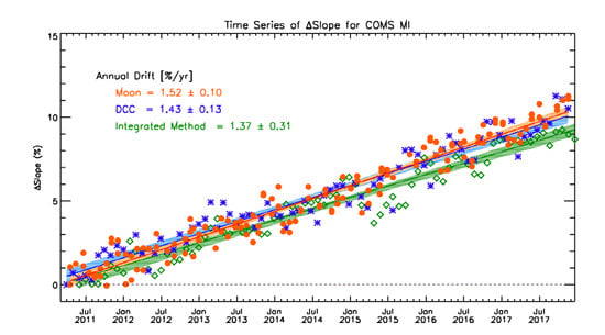
Figure 4 shows a time series of SlopeROLO (Equation (8)), which was rescaled against the first lunar observation using Equation (11),
Almost all results were fitted on the linear regression line. Lunar calibration results were compared with vicarious calibration results using DCC. Figure 4 shows a comparison between estimations of two calibration methods with respect to visible channel degradation of the COMS imager: Moon (orange dot) and DCC (blue asterisk), where DCC is a vicarious calibration method using a radiative transfer simulation developed by Sohn et al. [7].
It was noted that DCC overshot the tropical tropopause layer when cold brightness temperature appeared at the infrared window channel (e.g., 11 μm); this result assumes that the infrared channel was already well calibrated using other independent devices. After selecting DCC targets, typical optical properties were assumed as inputs to the RTM, based on an examination of DCC properties using MODIS cloud products. Reference values of sensor-reaching radiances were then produced from theoretical calculations, and these values were compared with Level 1B radiance products for calibration monitoring [7,31]. The bulk scattering properties for ice particles [32,33] were used as a scattering database in the RTM [7]. The two methods showed very similar annual drift values of 1.52 ± 0.10% per year and 1.43 ± 0.13% per year for Moon and DCC, respectively.
In addition to using the DCC method for comparison, three different earth targets were used (ocean, desert, and water cloud) to consider the wide reflectance range from the ocean’s surface around longitude 70°E–165°E and latitude 30°S–25°N as well as from a water cloud around longitude 128±40°E and latitude 40°S–40°N [7,31]. All three targets used RTM-calculated results as the calibration reference; inputs were MODIS products and NCEP (National Centers for Environmental Prediction)/NCAR(National Centers for Atmospheric Research) reanalysis data, such as TPW, UWIND, and VWIND. In this respect, each method was independent. Slopes were calculated using all three targets. An integrated method combining desert, ocean, and water cloud showed a similar annual drift value of 1.37 ± 0.31% per year.
3.4. Uncertainty Assessments
COMS-visible channel calibration showed clear temporal trends in spite of seasonal variations and time series scatters. However, several error sources affected the absolute values of the retrieved annual drift values. Therefore, before interpreting long-term calibration results from the visible channel with lunar observations, a sensitivity analysis was required to quantify their individual contributions to the degradation trend.
The magnitudes of uncertainties and their influence on long-term calibration stability were investigated with a predominant focus on the ratio between measured and modeled lunar irradiances. However, the selection of on-Moon pixels required a threshold value to discriminate between Moon and space pixels. This was not the same value as that of the space counter, as the value was retrieved near Moon disk pixels (see Appendix A.1.1). According to the sensitivity test, the uncertainty caused by different threshold values was within 0.01% per year of its annual drift. However, these conditions cannot be ignored. In addition, common criteria cannot be employed to calculate measured irradiances with respect to lunar calibration, as each detector has unique characteristics. Therefore, the uncertainty caused by moon pixel selection needed to be considered to determine the accuracy of lunar calibration. The selection of a higher threshold value increased the magnitude of annual drift, while that of lower value decreased the magnitude of sensor performance degradation.
Another uncertainty was that of phase angle dependence when retrieving irradiances. When i the phase angle was increased among the Sun, satellite, and Moon, the RMSEs of retrieved irradiance ratios (ΔIrr) were increased. For example, the retrieved annual drift between a phase angle of 0 and 30 was −1.26 ± 0.12% per year, while the value between 60° and 90° was −1.25 ± 0.24% per year. However, according to the perturbation test for the GIRO model, GIRO retrieved values are very stable. Irradiance variation was within 0.1% for a 10 × 10 km position perturbation. The large uncertainty in the irradiance ratio within increased phase angles was considered to be related to a combination of on-Moon pixel selection and model performance. There was a small total number of Moon pixels and the boundary between the Moon and space was not clear enough at large phase angles.
4. Discussion
Long-term monitoring of COMS MI visible channel calibration was conducted using Moon observation data from April 2011 to December 2017 under GSICS frameworks. Annual drift using Moon observations and the GIRO model was 1.52 ± 0.10% per year; this value is comparable with that of the DCC and integration method (i.e., 1.43 ± 0.13% per year and 1.37 ± 0.31% per year, respectively). Notably, the lunar calibration result was in good agreement with that provided by vicarious calibration, such as the DCC and integration method [13,16]. However, the COMS MI annual drift value was different from that of other sensors (such as MSG/VIS06 of 0.48 ± 0.02% per year [26] and MTSAT-2 of 2.71 ± 0.15% per year) [30], as the sensor degradation rate depended on factors such as detector characteristics and the exposed space environment. This appears reasonable with respect to the relatively broad range of annual drift values, as the expected drifts were between one and several percent over five years, despite the very stable design of the imaging instrument [21].
The irradiance ratio between GIRO and lunar observations showed strong seasonal variation due to seasonal variation in the phase angle of the Moon. Furthermore, the phase angle of the Moon showed a similar pattern every half year, which was related to Moon observation attitude and time. Phase angle dependence was corrected to remove seasonal variation of Moon irradiance. After angle correction was applied, the annual drift value remained the same but the standard deviation was reduced from 0.78 to 0.51.
Sensitivity tests were conducted to investigate and quantify uncertainties that affected calibration accuracy using Moon observation and the GIRO model; these are described in Appendix A. In the sensitivity test described in Appendix A, the calibration uncertainty (around 7%), in accordance with the threshold used to determine moon pixels, was driven by measured irradiances by the MI (IInstrument). The uncertainty contained errors that were driven by the pixel numbers on the boundary area between the Moon and space. In addition, the uncertainty in calculating irradiance (Equation (7)) was derived from a cumulative error in determining the detector counts corresponding to photons from the Moon. This accounted for all detector artifact corrections and calibration uncertainties and was combined with the uncertainty of sky background subtraction. Summed irradiances were corrected for point-spread effects in the ground-based lunar observations; an analytic correction was developed from radial profiles of the sky background for a selected set of lunar images acquired over the ROLO operational range of phase angles.
Uncertainty in lunar model absolute accuracy when scaled against SI (Système International d’unités) radiometric units remained at a level of 5–10%. Inter-band irregularities in model outputs required an adjustment to produce a smooth reflectance spectrum that was expected for the Moon. Therefore, the model’s reliability for predicting irradiance variation with geometry far exceeded absolute accuracy; reducing such variation is a high priority to enable the use of the Moon as a transfer standard for inter-calibration of instruments which have dissimilar bands.
5. Conclusions
This study reports the long-term characteristics of the COMS MI visible channel for the first time through the application of GSICS concepts, implementation of GIRO, and the use of moon observation data from April 2011 to December 2017. Results indicated that the irradiance ratio between GIRO and lunar observations of COMS MI showed strong seasonal variation due to seasonal variation in the phase angle of the Moon. Furthermore, the phase angle of the Moon showed a similar pattern every half year, which was related to Moon observation attitude and time. For COMS MI, the number of Moon observations was limited because of the attenuation tendency with respect to the limited phase angle range. However, when Geo-KOMPSAT-2A (Geostationary-Korea Multi-Purpose Satellite-2A) AMI (Advanced Meteorological Imager), the next generation geostationary satellite of KMA, is launched at the end of 2018, the Moon phase angle will be further subdivided through an analysis of the degradation ratio. It is anticipated that Moon observation data will be obtained more frequently than with COMS MI. Therefore, it is expected that the effect of seasonal variation on the phase angle will be reduced.
Author Contributions
T.-H.O. processed COMS MI Moon observation data, plotted, and analyzed results of Moon calibration, and prepared the manuscript. D.K. formulated and directed the methodology, validation, results, and analysis. Both authors contributed to the methodology, validation, results, analysis, and reviewed the manuscript.
Acknowledgments
This study was supported by the project entitled “Development of Meteorological Satellite Operation and Application Technology” of the KMA/NMSC (Korea Meteorological Administration/National Meteorological Satellite Center).
Conflicts of Interest
The authors declare no conflict of interest.
Appendix A
Appendix A.1. Sensitivity Test
The lunar reflectance phase curve is generally known to be a smooth function with any wavelength. Small variations were seen in the model results, which were a result of the effects of lunar librations; a corresponding structure was expected and observed in measured reflectance. However, measurement results varied far more than what can be accounted for by libration contribution. Therefore, the observed scatter must have originated with the irradiance measurements, as calculated using (1). Several potential sources of this scatter have been identified and are described here.
A sensitivity test was conducted to determine on-Moon pixels and to determine the threshold for Moon pixel selection for use in calculating Moon-observed irradiance (IInstrument) for the visible channel using COMS MI Moon observation data. It was also used to determine the optimum Moon image size and the pixels used in lunar calibration from those in the entire observation area.
Appendix A.1.1. Defining on-Moon Pixels
The sensitivity test used to select only Moon pixels in the Moon image area was conducted using Moon observation data obtained from April 2011 to December 2016. The mean and the standard deviation (σ) of the space area were calculated by selecting the upper and the lower 10 lines of the Moon image in this period. The mean of the selected space area was approximately 795.18 and the standard deviation was approximately 22.33. Using the mean and the standard deviation and relating with the confidence interval, the thresholds were defined as 800, 820, 840, and 860. Figure A1 shows the Moon pixel area according to the observed Moon image taken on 19 August 2016, 03:28:45 UTC, and 12 July 2016, 22:43:35 UTC, respectively.
Figure A1.
Differences in Moon pixels due to the threshold value on selected Moon area (560 × 330). (Top) Moon observation image and associated threshold values of: (a) 800, (b) 820, (c) 840, and (d) 860.
Figure A1.
Differences in Moon pixels due to the threshold value on selected Moon area (560 × 330). (Top) Moon observation image and associated threshold values of: (a) 800, (b) 820, (c) 840, and (d) 860.

As shown in Figure A1, the Moon pixel area differed according to the Moon pixel threshold selected. In particular, it demonstrates that, when the phase angle was 70° or more (as on 12 July 2016, when the moon was a half-Moon), there were significant differences among the selection of moon pixels according to boundary values. Differences in Moon pixel areas according to threshold values affected the irradiance of the Moon and affected the degradation ratio (P(t)) of the visible channel.
Figure A2 shows the irradiance ratio (P(t)) obtained from threshold values of (800, 820, 840, and 860) and total pixels in selected Moon image areas. From this, it is evident that the degradation ratio differed according to the threshold value. In particular, the radiance of Moon observations with phase angles up to 70° appeared sharp or decayed.
To eliminate the phenomenon whereby the radiance ratio changed according to the threshold, and to prevent occurrence of the threshold changing as a result of performance degradation of the visible channel with the passing of time, it was necessary to monitor the performance of the COMS MI visible channel using entire pixels. In this test, the threshold was defined as 860 digital counts and the Moon region was selected to minimize the effect from both space and Earth pixels as well as to calculate Moon radiance for all the pixels in the selected Moon region.
Figure A2.
Degradation ratios for threshold values used in selected Moon image areas.

Appendix A.1.2. Phase Angle Dependence
The results presented in Figure 3 and Figure 4 show periodicity in changes of the degradation ratio (P(t)) for the COMS MI visible channel. Moon irradiance caused errors with respect to the Moon’s absolute phase angle. The phase angles of lunar images observed from COMS MI had similar patterns every year, which created seasonal variation in the irradiance ratio.
The degradation tendency of the visible channel of COMS MI was analyzed by dividing it into three regions according to the phase angle range. This allowed an observation of changes in the degradation ratio according to the Moon phase angle. Table A1 shows Moon observation images and phase angles in the three ranges of absolute phase angles.

Table A1.
Example of Moon image with three phase angle ranges.
| Absolute Phase Angle Range (Degree) | Observation Time (UTC) | Moon Images | Phase Angle (Degree) |
|---|---|---|---|
| |phase angle| ≤ 30 | 2016-08-1903:28:45 |  | 9.3 |
| 30 < |Phase angle| ≤ 60 | 2016-10-1301:13:34 |  | −41.5 |
| 60 < |phage angle| | 2016071221:28:45 |  | −81.5 |
Figure A3 shows the attenuation tendency of the COMS MI visible channel according to the phase angle range of the Moon.
Figure A3.
Degradation ratio as a result of phase angle range of COMS MI; (a) absolute phase angle ≤ 30°, (b) 30° < absolute phase angle ≤ 60° and (c) 60° < absolute phase angle.
Figure A3.
Degradation ratio as a result of phase angle range of COMS MI; (a) absolute phase angle ≤ 30°, (b) 30° < absolute phase angle ≤ 60° and (c) 60° < absolute phase angle.

As shown in Figure A3, the degradation ratio tendency variesd depending on the absolute phase angle range.
In Table A2, the degradation ratio was the same when the absolute phase angle was less than 30°, although there are differences of approximately of 0–8% with a Moon degradation ratio of −1.35% per year, with respect to the result of Equation (9) using a full Moon image.
Table A2.
Difference in degradation ratio of COMS visible channel due to absolute phase angle range.
Table A2.
Difference in degradation ratio of COMS visible channel due to absolute phase angle range.
| Absolute Phase Angle Range (Degree) | No. of Moon Observation Data | Degradation Ratio (%/year) |
|---|---|---|
| |phase angle ≤ 30| | 60 | −1.35 ± 0.09 |
| |30 < Phase angle ≤ 60| | 59 | −1.41 ± 0.11 |
| |60 < phage angle| | 27 | −1.25 ± 0.27 |
| All phase angle | 146 | −1.35 ± 0.10 |
Appendix B
ROLO Lunar Irradiance Model Coefficients of COMS MI
Eight coefficients were constant over all wavelengths in Equation (5): c1, c2, c3, c4, p1, p2, p3, p4; where
c1 = 0.00034115 (deg−1), c2 = −0.0013425 (deg−1), c3 = 0.00095906 (deg−1 rad−1), c4 = 0.00066229 (deg−1 rad−1),
p1 = 4.06054 (deg), p2 = 12.8802 (deg), p3 = −30.5858 (deg), p4 = 105.242 (deg),
Table A3 lists ROLO Lunar Irradiance Model Coefficients for the COMS MI visible wavelength given by ROLO [30]; these values were interpolated to the instrument band using a linear interpolation.
Table A3.
ROLO Lunar Irradiance Model Coefficients [29].
Table A3.
ROLO Lunar Irradiance Model Coefficients [29].
| Wavelength (nm) | a0 (Constant) | a1 (rad−1) | a2 (rad−2) | a3 (rad−3) | b1 (rad−1) | b2 (rad−3) | b3 (rad−5) | d1 (Exponent 1) | d2 (Exponent 2) | d3 (Cosine) |
|---|---|---|---|---|---|---|---|---|---|---|
| 544.0 | −2.13864 | −1.60613 | 0.27886 | −0.16426 | 0.03833 | 0.01189 | −0.00390 | 0.37190 | −0.10629 | 0.01428 |
| 549.1 | −2.10782 | −1.66736 | 0.41697 | −0.22026 | 0.03451 | 0.01452 | −0.00517 | 0.36814 | −0.09815 | 0.00000 |
| 553.8 | −2.12504 | −1.65970 | 0.38409 | −0.20655 | 0.04052 | 0.01009 | −0.00388 | 0.37206 | −0.10745 | 0.00347 |
| 665.1 | −1.88914 | −1.58096 | 0.30477 | −0.17908 | 0.04415 | 0.00983 | −0.00389 | 0.37141 | −0.13514 | 0.01248 |
| 693.1 | −1.89410 | −1.58509 | 0.28080 | −0.16427 | 0.04429 | 0.00914 | −0.00351 | 0.39109 | −0.17048 | 0.01754 |
| 703.6 | −1.92103 | −1.60151 | 0.36924 | −0.20567 | 0.04494 | 0.00987 | −0.00386 | 0.37155 | −0.13989 | 0.00412 |
| 745.3 | −1.86896 | −1.57522 | 0.33712 | −0.19415 | 0.03967 | 0.01318 | −0.00464 | 0.36888 | −0.14828 | 0.00958 |
| 763.7 | −1.85258 | −1.47181 | 0.14377 | −0.11589 | 0.04435 | 0.02000 | −0.00738 | 0.39126 | −0.16957 | 0.03053 |
| 774.8 | −1.80271 | −1.59357 | 0.36351 | −0.20326 | 0.04710 | 0.01196 | −0.00476 | 0.36908 | −0.16182 | 0.00830 |
References
- Hewison, T.J.; Wu, X.; Yu, F.; Tahara, Y.; Hu, X.; Kim, D.; Koenig, M. GSICS Inter-Calibration of Infrared Channels of Geostationary Imagers Using Metop/IASI. IEEE Trans. Geosci. Remote Sens. 2013, 51, 1160–1170. [Google Scholar] [CrossRef]
- Kim, D.; Ahn, M.H. Introduction to the in-orbit-test and its performance of the first meteorological imager of the Communication Ocean, and Meteorological Satellite. Atmos. Meas. Tech. 2014, 7, 2471–2485. [Google Scholar] [CrossRef]
- Goldberg, M.; Ohring, G.; Butler, J.; Cao, C.; Dalta, R.; Doelling, D.; Gaertner, V.; Hewison, T.; Iacovazzi, B.; Kim, D.; et al. The global space-based inter-calibration system (GSICS). Bull. Am. Meteorol. Soc. 2011, 92, 468–475. [Google Scholar] [CrossRef]
- Xiong, X.; Sun, J.; Espositio, J.; Guenther, B.; Barnes, W. MODIS reflective solar bands calibration algorithm and on-orbit performance. Proc. SPIE–Opt. Remote Sens. Atmos. Clouds III 2002, 4891. [Google Scholar] [CrossRef]
- Cao, C.; De Luccia, F.; Xiong, X.; Wolfe, R.; Weng, F. Early on-orbit performance of the Visible Infrared Imaging Radiometer Suite (VIIRS) onboard the Suomi National Polar-orbiting Partnership (S-NPP) satellite. IEEE Trans. Geosci. Remote Sens. 2014, 52. [Google Scholar] [CrossRef]
- Sohn, B.-J.; Ham, S.H. Possibility of the visible-channel calibration using deep convective clouds overshooting the TTL. J. Appl. Meteorol. Climatol. 2009, 48, 2271–2283. [Google Scholar] [CrossRef]
- Cosnefroy, H.; Leroy, M.; Briottet, X. Selection and characterization of Saharan and Arabian desert sites for the calibration of optical satellite sensors. Remote Sens. Environ. 1996, 58, 101–114. [Google Scholar] [CrossRef]
- Doelling, D.; Nguyen, L.; Minnis, P. On the use of deep convective clouds to calibrate AVHRR data. In Proceedings of the SPIE 49th Annual Meeting, Earth Observing Systems IX Conference, Denver, CO, USA, 2–6 August 2004. [Google Scholar]
- Doelling, D.; Minnis, P.; Nguyen, L. Calibration comparisons between SEVIRI, MODIS and GOES data. In Proceedings of the MSG RAO Workshop, Salzburg, Austria, 9–10 September 2004. [Google Scholar]
- Fougnie, B.; Henry, P.; Morel, A.; Antoine, D.; Montagner, F. Identification and characterization of stable homogeneous ocean zones: Climatology and impact on in-flight calibration of space sensor over Rayleigh scattering. Proceedings of Ocean Optics XVI, Santa Fe, New Mexico, 18–22 November 2002. [Google Scholar]
- Hagolle, O.; Nicolas, J.; Fougnie, B.; Cabot, F.; Henry, P. Absolute calibration of VEGETATION derived from an interband method based on the Sun glint over ocean. IEEE Trans. Geosci. Remote Sens. 2002, 42, 1472–1481. [Google Scholar] [CrossRef]
- Wu, X.; Stone, T.C.; Yu, F.; Han, D. Vicarious calibration of GOES Imager visible channel using the Moon. Proc. SPIE Earth Obs. Syst. XI 2006, 6296. [Google Scholar] [CrossRef]
- Yu, F.; Wu, X. NOAA Operational Implementation of DCC Correction. In Proceedings of the GSICS Annual Meeting, Darmstadt, Germany, 10–14 March 2014; Available online: https://gsics.nesdis.noaa.gov/wiki/Development/20140324 (accessed on 2 May 2016).
- Doelling, D.; Morstd, D.; Bhatt, R.; Scarino, B. Algorithm Theoretical Basis Document (ATBD) for Deep Convective Cloud (DCC), 2011. Available online: https://gsics.nesdis.noaa.gov/pub/Development/AtbdCentral/GSICS_ATBD_DCC_NASA_2011_09.pdf (accessed on 2 May 2016).
- Yu, F.; Wu, X. An integrated method to improve the GOES Imager visible radiometric calibration accuracy. Remote Sens. Environ. 2015, 164, 103–113. [Google Scholar] [CrossRef]
- Kieffer, H.H.; Wildey, R.L. Absolute calibration of Landsat instruments using the Moon. Photogramm. Eng. Remote Sens. 1985, 51, 1391–1393. [Google Scholar]
- Kieffer, H.H.; Wildey, R.L. Establishing the Moon as a spectral radiance standard. J. Atmos. Ocean. Technol. 1996, 13, 360–375. [Google Scholar] [CrossRef]
- Anderson, J.M.; Becker, K.J.; Kieffer, H.H.; Dodd, D.N. Real-time control of the Robotic Lunar Observatory telescope. Publ. Astron. Soc. Pac. 1996, 111, 737–749. [Google Scholar] [CrossRef]
- Anderson, J.M.; Kieffer, H.H. New Views of the Moon II: Understanding the Moon through the Integration of Diverse Datasets; Gaddis, L., Shearer, C.K., Eds.; LPI: Houston, TX, USA, 1999; Volume 2. [Google Scholar]
- Stone, T.C.; Kieffer, H.H. Absolute Irradiance of the Moon for On-orbit Calibration. Proc. SPIE 2002, 4881, 287–298. [Google Scholar]
- Kieffer, H.H.; Stone, T.C. The spectral irradiance of the Moon. Astron. J. 2005, 129, 2887–2901. [Google Scholar] [CrossRef]
- Stone, T.C.; Kieffer, H.H.; Anderson, J.M. Status of Use of Lunar Irradiance for On-orbit Calibration. Proc. SPIE 2002, 4483, 165–175. [Google Scholar]
- Barnes, R.A.; Eplee, R.E., Jr.; Patt, F.S.; Kieffer, H.H.; Stone, T.C.; Meister, G.; Butler, J.J.; McClain, C.R. Comparison of SeaWiFS measurements of the Moon with the US Geological Survey lunar model. Appl. Opt. 2004, 43, 5838–5854. [Google Scholar] [CrossRef] [PubMed]
- EUMETSAT, High Level Description of the GIRO Application and Definition of the Input/Output Formats, 2015. Available online: http://gsics.atmos.umd.edu/bin/view/Development/LunarWorkArea (accessed on 2 February 2015).
- Stone, T.C.; Rossow, W.B.; Ferrier, J.; Hinkelman, L.M. Evaluation of ISCCP multisatellite radiance calibration for geostationary imager visible channels using the Moon. IEEE Trans. Geosci. Remote Sens. 2003, 51, 1255–1266. [Google Scholar] [CrossRef]
- Viticchie, B.; Wagner, S.C.; Hewison, T.J.; Stone, T.C.; Nain, J.; Gutierrez, R.; Muller, J.; Hanson, C. Lunar calibration of MSG/SEVIRI solar channels. In Proceedings of the EUMETSAT Meteorological Satellite Conference, Vienna, Austria, 16–20 September 2013. [Google Scholar]
- Eplee, R.E.; Meister, G.; Patt, F.S.; Barnes, R.A.; Bailey, S.W.; Franz, B.A.; McClain, C.R. On-orbit calibration of SeaWiFS. Appl. Opt. 2012, 51, 8702–8730. [Google Scholar] [CrossRef] [PubMed]
- Seo, S.B.; Yong, S.S. Moon ROLO irradiance calculation with coordinate transforms for detectors’ performance analysis of geostationary visible channel imagers. In Proceedings of the International Symposium on Remote Sensing, Pusan, Korea, 16–18 April 2014. [Google Scholar]
- Ledez, C. MI Radiometric Model, Astrium and KARI Proprietary Information; COMS.TN.00116.DP.T.ASTR; Astrium: Paris, France, 2011; pp. 30–45. [Google Scholar]
- Takahashi, M. Visible Channel Calibration of the JMA’s Geostationary Satellites Using the Moon Images. In Proceedings of the 2014 EUMETSAT Meteorological Satellite Conference, Geneva, Switzerland, 22–26 September 2014. [Google Scholar]
- Ham, S.-H.; Sohn, B.J. Assessments of the calibration performance of satellite visible channels using cloud targets: Application to Meteosat-8/9 and MTSAT-1R. Atmos. Chem. Phys. 2010, 10, 11131–11149. [Google Scholar] [CrossRef]
- Baum, B.A.; Heymsfield, A.J.; Yang, P.; Bedka, S.T. Bulk scattering models for the remote sensing of ice clouds. Part I: Microphysical data and models. J. Appl. Meteorol. 2005, 44, 1885–1895. [Google Scholar] [CrossRef]
- Baum, B.; Yang, P.; Heymsfield, A.J.; Platnick, S.; King, M.D.; Hu, Y.-X.; Bedka, S.T. Bulk scattering models for the remote sensing of ice clouds. Part II: Narrowband models. J. Appl. Meteorol. 2005, 44, 1896–1911. [Google Scholar] [CrossRef]
Figure 1.
Level 1A (Local Area (LA) mode) Moon observation data (a) Normal Moon observation data (b) Moon image with Earth on the edge of LA Image (1–2 times annually).
Figure 1.
Level 1A (Local Area (LA) mode) Moon observation data (a) Normal Moon observation data (b) Moon image with Earth on the edge of LA Image (1–2 times annually).

Figure 2.
Temporal trend of COMS MI visible channel calibration from April 2011 to March 2017. Colors represent Moon phase angles and orange shades represent the 95% confidence interval of the linear regression.
Figure 2.
Temporal trend of COMS MI visible channel calibration from April 2011 to March 2017. Colors represent Moon phase angles and orange shades represent the 95% confidence interval of the linear regression.

Figure 3.
(a) Difference between degradation ratio and regression value (R(IInstrument/IROLO) − R′[y = mx + b] (%)). The annual difference between degradation ratio and regression value is evident and shows a clear seasonal variation. (b) Variations in phase angle annually from April 2011 to December 2017 (the year is divided into two parts: January to June and July to December.

Figure 4.
Comparison of visible channel degradation of COMS imager among several calibration methods: Moon (orange dot), DCC (using RTM) (blue asterisk) and integrated method (green diamond) from April 2011 to December 2017. The shades represent the 95% confidence interval of the linear regression for moon (orange shade) and DCC (light blue shade).

Table 1.
Characteristics of COMS meteorological Imager.
| Channel | Spectral Range (μm) | Central Wavelength (μm) | IFOV 1 (μrad) | Spatial Resolution (km) | Input Range | SNR 2 (VIS) and NEdT 3 (IR) |
|---|---|---|---|---|---|---|
| VIS | 0.55–0.8 | 0.675 | 28 × 28 | 1 | 0–115% albedo | 170:1 at 100% albedo 10:1 at 5% albedo |
| SWIR | 3.5–4.0 | 3.75 | 112 × 112 | 4 | 4–330 K | 0.10 K at 300 K 5.70 K at 220 K |
| WV | 6.5–7.0 | 6.75 | 112 × 112 | 4 | 4–330 K | 0.12 K at 300 K 0.85 K at 220 K |
| IR1 | 10.3–11.3 | 10.8 | 112 × 112 | 4 | 4–330 K | 0.12 K at 300 K 0.40 K at 220 K |
| IR2 | 11.5–12.5 | 12.0 | 112 × 112 | 4 | 4–350 K | 0.20 K at 300 K 0.48 K at 220 K |
1 IFOV: Instrantaneous Field of View; 2 SNR: Signal-to-Noise Ratio; 3 NEdT: Noise Equivalent differential Temperature.
Table 2.
Characteristics of COMS MI Moon Observation Data.
| Satellite | Time Coverage | Moon Observations (Times) | Channel | Absolute Phase Angle Range (Degree) | Useful Observation for Calibration | ||
|---|---|---|---|---|---|---|---|
| COMS MI | April 2011–December 2017 | 152 | Visible (0.6 μm) | 0–90 | 0–30 | 146 | 60 |
| 31–60 | 59 | ||||||
| 61–90 | 27 | ||||||
© 2018 by the authors. Licensee MDPI, Basel, Switzerland. This article is an open access article distributed under the terms and conditions of the Creative Commons Attribution (CC BY) license (http://creativecommons.org/licenses/by/4.0/).
Share and Cite
MDPI and ACS Style
Oh, T.-H.; Kim, D. COMS Visible Channel Calibration Using Moon Observation Data. Remote Sens. 2018, 10, 726. https://0-doi-org.brum.beds.ac.uk/10.3390/rs10050726
AMA Style
Oh T-H, Kim D. COMS Visible Channel Calibration Using Moon Observation Data. Remote Sensing. 2018; 10(5):726. https://0-doi-org.brum.beds.ac.uk/10.3390/rs10050726
Chicago/Turabian StyleOh, Tae-Hyeong, and Dohyeong Kim. 2018. "COMS Visible Channel Calibration Using Moon Observation Data" Remote Sensing 10, no. 5: 726. https://0-doi-org.brum.beds.ac.uk/10.3390/rs10050726
Note that from the first issue of 2016, this journal uses article numbers instead of page numbers. See further details here.