Hyperspectral Anomaly Detection via Discriminative Feature Learning with Multiple-Dictionary Sparse Representation


1
Center for OPTical IMagery Analysis and Learning (OPTIMAL), Xi’an Institute of Optics and Precision Mechanics, Chinese Academy of Sciences, Xi’an 710119, Shaanxi, China
2
University of Chinese Academy of Sciences, Beijing 100049, China
3
School of Computer Science, and Center for OPTical IMagery Analysis and Learning (OPTIMAL), and Unmanned System Research Institute (USRI), Northwestern Polytechnical University, Xi’an 710072, Shaanxi, China
*
Author to whom correspondence should be addressed.
Remote Sens. 2018, 10(5), 745; https://0-doi-org.brum.beds.ac.uk/10.3390/rs10050745
Submission received: 31 March 2018
/
Revised: 4 May 2018
/
Accepted: 10 May 2018
/
Published: 11 May 2018
(This article belongs to the Section Remote Sensing Image Processing)
Abstract
:Most hyperspectral anomaly detection methods directly utilize all the original spectra to recognize anomalies. However, the inherent characteristics of high spectral dimension and complex spectral correlation commonly make their detection performance unsatisfactory. Therefore, an effective feature extraction technique is necessary. To this end, this paper proposes a novel anomaly detection method via discriminative feature learning with multiple-dictionary sparse representation. Firstly, a new spectral feature selection framework based on sparse presentation is designed, which is closely guided by the anomaly detection task. Then, the representative spectra which can significantly enlarge anomaly’s deviation from background are picked out by minimizing residues between background spectrum reconstruction error and anomaly spectrum recovery error. Finally, through comprehensively considering the virtues of different groups of representative features selected from multiple dictionaries, a global multiple-view detection strategy is presented to improve the detection accuracy. The proposed method is compared with ten state-of-the-art methods including LRX, SRD, CRD, LSMAD, RSAD, BACON, BACON-target, GRX, GKRX, and PCA-GRX on three real-world hyperspectral images. Corresponding to each competitor, it has the average detection performance improvement of about , , , , , , , , , and respectively. Extensive experiments demonstrate its superior performance in effectiveness and efficiency.
1. Introduction
Hyperspectral image (HSI) delivers rich spectral information [1] that usually covers a large spectral range almost from visible to mid-infrared. These spectra are divided into hundreds of approximately continuous and very narrow spectral bands which have a strong ability to precisely characterize different objects and accurately recognize the subtle differences between surface materials [2,3]. Benefiting from its high spectral resolution, hyperspectral image has been successfully used in many applications [4], such as target detection [5,6], image classification [7,8], band selection [9,10], and hyperspectral unmixing [11,12].
Target detection is one of the hottest topics in remote sensing. Anomaly detection is a special category of target detection, in which no prior information about the spectra of both the target of interest and the background is known [13]. Through analyzing the surrounding background information, and comparing the spectral difference, a pixel will be regarded as an abnormal target when its spectra significantly deviate from the spectra of its reference background [13]. Requiring no information about the scene makes anomaly detection have been widely used in many practical applications [14,15,16], such as agriculture [17], geology [18], public security [19,20], etc.
Hyperspectral anomaly detection has attracted researchers’ great interest, and many methods have been proposed in recent decades [21,22,23,24,25]. Generally, most of these methods aim to make a more accurate background estimation or enhance the difference between background and anomaly by using some criteria or assumptions. The famous Reed-Xiaoli (RX) [26] algorithm is the most typical method, which is based on a hypothesis test. It assumes a multivariate normal distribution for the background and formates two conditional probability functions corresponding to the conditions of within and without anomalies [27]. In the specific implementation process, a Mahalanobis distance is computed to estimate the difference between the pixel under test and its reference background. The RX method contains two versions according to the scope of the reference background [28]. When the local surrounding region of a pixel under test is regarded as the background, it will be the local RX (LRX). While when the whole image scene is treated as the background, it will be defined as the global RX (GRX).
However, in fact this multivariate normal distribution is hard to be satisfied and is too simple to accurately characterize a real hyperspectral image, because the image scene usually covers a large scale of ground containing many different materials [29]. The computation of Mahalanobis distance is also inaccurate, because it involves computing the background mean and covariance matrix which will be affected by anomalies. Specifically speaking, for the LRX method, although it usually adopts a sliding dual window [30] to relieve anomalies’ effects on background estimation, it can hardly eliminate anomalies’ existence from the reference background. Besides, LRX also has a small sample problem and suffers heavy time computation. As for the GRX method, it generally directly estimates the background statistical property on the whole image without using a sliding technique. Thus it is much more efficient than LRX method. But the inadequate distribution assumption is also the main reason that limits its performance.
In order to address these problems involved in RX, many methods have been proposed in recent two decades. Some of them aim to obtain a more purer background in order to make an accurate estimation. For example, the random-selection-based anomaly detector (RSAD) [31] uses a random selection strategy to select some representative background pixels, then a better background set can be finally obtained after implementing the selection procedure several times. Zhao et al. propose a method named robust nonlinear anomaly detection (RNAD) [32] which utilizes a regression detection strategy to purify the background and suppress the contamination of anomalies. Some of them adopt a kernel technique to nonlinearly map the hyperspectral data into a high-dimensional feature space in order to enhance the discrimination between the target and the background. One typical kernel-based method is kernel-RX (KRX) which is a nonlinear version of RX method [33]. The support vector data description (SVDD) [34] method is a nonparametric kernel-based anomaly detector. It constructs an enclosing hypersphere to envelope the background in the high-dimensional feature space. In addition, a more complex background distribution assumption is also proposed in order to describe the hyperspectral image more accurately. It has a hypothesis that the background contains multiple classes with different distributions [35]. For example, the cluster-based anomaly detector (CBAD) [36] divides the hyperspectral image into different clusters and makes the assumption that each of background class obeys a multivariate normal distribution.
In recent years, many representation-based methods [37,38,39,40,41,42,43,44] have been proposed. For these methods, the background is supposed to be well represented by some representative materials’ spectra or basis vectors. For instance, the collaborative-representation-based detector (CRD) [45] which is also a sparse representation-based detector (SRD), considers that a background pixel can be approximately linearly represented by its neighbors, while an anomaly can not satisfy this condition. Yuan et al. [38] propose analyzing the local sparsity divergence to detect anomalies, in which a sliding window strategy is directly used to obtain the sparsity difference between abnormal targets and background. Wang et al. [40] impose the sparsity constraint for abnormal pixels and simultaneously use a minimum volume constraint in the matrix decomposition process in order to analyze the background. Zhao et al. [46] propose a hyperspectral anomaly detection method through constructing a sparsity score estimation framework. By using the sparse representation technique, they compute the atom usage probability according to the learned dictionary and further transform the probability into sparsity score as abnormal degree. In order to select some most active dictionary bases to better describe the background, Li et al. [43] propose an anomaly detector by using the background joint sparse representation. Since the background usually lies in a low-dimensional subspace, it tends to have a low rank property. Therefore, a low-rank and sparse matrix decomposition-based mahalanobis distance method (LSMAD) [41] is proposed to accurately calculate the background statistics after using the low-rank constraint to obtain the background matrix. In order to accurately represent the characteristics of different material spectra, Qu et al. [39] take both the spectral unmixing and low-rank decomposition into consideration. They regard the abundance vectors as new features after using spectral unmixing technique, and then design a low-rank decomposition approach to detect anomalies.
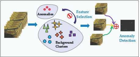
In this paper, we want to propose a novel anomaly detection method from the view of discriminative feature extraction. Despite the high spectral resolution delivering rich information, its high spectral dimension and complicated spectral correlation commonly have great effects on the anomaly detection performance when a detector is directly implemented on the original whole spectra. Therefore, it is necessary to pick out some representative spectra to recognize anomalies. Actually, the spatial information is also important to analyze a remote sensing image. For example, Chen et al. [47] incorporate the spatial information in their sparsity-based hyperspectral image classification model. Dao et al. [48] also jointly consider the spatial and spectral information to constrain the group sparsity. However, in this work, we mainly focus on the spectral information in order to obtain the discriminative spectral feature. The spatial information will be deeply studied in the future work. Generally, there are a variety of materials belonging to different categories in the background. Each category has its own specifically significant spectra. Consequently, we can pick out a particular group of representative spectra for each category to enlarge the deviation of anomaly from each background class. In other words, each background category can be regarded as an observer, and each of them selects some salient spectra which are greatly different from anomaly’s from its own perspective. Inspired by this idea, we propose a novel hyperspectral anomaly detection method based on sparse representation through constructing multiple dictionaries to learn discriminative features. The sparse representation is used to describe the relationships between different spectra. More specifically, each band vector can be sparsely represented by a few of salient band bases, and these corresponding data bases will be selected as the new spectral features. These discriminative features are expected to strengthen the disparity between background and anomaly in order to further improve the detection performance. The main contributions of the proposed method can be summarized as follows. Bulleted lists look like this:
- (1)
- Instead of simply combining the feature selection technique with anomaly detection method, a new spectral feature selection framework based on sparse representation is designed, which is closely guided by the anomaly detection task and they can reciprocally affect each other.
- (2)
- Not only using the background information but also applying some anomalies’ spectral knowledge, the representative spectra which can significantly enlarge anomaly’s deviation from background are picked out by minimizing the residues between their recovery errors.
- (3)
- Through comprehensively considering the virtues of different groups of representative features selected from multiple dictionaries, a global multiple-view detection strategy is presented to jointly improve the detection accuracy.
2. Our Method
In this paper, we detect abnormal targets from the view of discriminative feature extraction. The philosophy of our method is based on that selecting some representative spectra to enlarge the difference between background and anomaly can significantly improve the anomaly detection performance, because the original whole spectra usually have characteristics of high spectral dimension and complex spectral correlation. We take advantage of sparse representation to construct the discriminative feature selection framework, and further comprehensively apply the background and anomaly knowledge learned from a simple preliminary detection to constrain this feature extraction process. There are two important procedures: (1) multiple-dictionary sparse feature extraction and (2) global multiple-view anomaly detection.
First, we design the multiple-dictionary sparse feature extraction process which is closely guided by the anomaly detection task. Considering the image scene covers various kinds of materials, multiple dictionaries are constructed to select different groups of representative features corresponding to different background categories. Moreover, in order to pick out these discriminative spectra which can significantly enlarge the disparity between background and anomaly, we minimize the residues between their spectra reconstruction errors. When finishing selecting a few groups of representative features, we further propose a global multiple-view anomaly detection strategy. Through comprehensively considering the virtues of different groups of representative features selected from multiple dictionaries, a global joint detection strategy is presented to fuse all the detection results generated by different background views in order to improve the detection accuracy. The proposed method will be introduced in detail in the following parts.
2.1. Multiple-Dictionary Sparse Feature Extraction
This part will introduce the multiple-dictionary sparse feature extraction method in detail. Considering that the rich spectral information with hundreds of spectra usually contains much redundant information and band correlation, a spectral band of a hyperspectral image is generally assumed to be linearly represented by some representative spectra. The sparse representation is a typical model to describe the relationships between spectra. In this paper, denotes the 2-D representation of a 3-D hyperspectral image, where m and n respectively correspond to the height and width of the hyperspectral image, is the total number of image pixels, B denotes the number of spectra, and denotes a spectral vector of one image band. Assuming that some desired spectral bands can construct a dictionary (s is the number of the desired bands), consequently, the traditional feature selection model based on sparse representation can be defined as follows.
where is the coefficient matrix, and is the regularized parameter. It should be noted that many different norms can be applied to constrain the coefficient matrix . Here, we utilize the commonly used mixed norm to guarantee that is sparse in rows. We expect to pick out some active spectra that can simultaneously accurately describe intrinsic characteristics of all the samples in . In addition, the norm of can be computed as
where is one element of and is a vector corresponding to the row of .
As stated above, the goal of traditional band selection is to select an appropriate band subset from the original band set of the hyperspectral image. It usually requires that the selected subset should have a good ability to describe the whole hyperspectral image. Nevertheless, it also requires that the difference between these selected bands should be large and the correlation should be small with some certain constraints at the same time [49]. But this feature selection is completely independent of any application tasks. Consequently it is hard to ensure the selected bands are appropriate for the subsequent tasks. Therefore, in this work we combine the anomaly detection with the feature selection closely and design a new spectral feature selection framework driven by anomaly detection. Through constructing this model, we expect these two tasks can mutually affect each other in order to pick out some representative bands which can satisfy the requirements of anomaly detection and further improve the detection performance.
For the anomaly detection task, the representative spectra which can enhance the difference between background and anomaly are expected to be picked out. Based on the sparse representation, if a band subset can well describe the background spectra but has larger reconstruction errors to represent the anomaly spectra, then this band set can be regarded as the representative band set in this work. When using these selected spectral features, an abnormal target will be more significant in the image scene and the detection performance will be improved. Inspired by this idea, we revise the traditional sparse feature selection method by introducing the background and the anomaly knowledge which can be learned from a simple preliminary detection. Our feature selection method guided by anomaly detection task can be formulated as
where is the background spectra set, and denotes the anomaly spectra set. Through minimizing the residues between background spectra reconstruction errors and anomaly spectra recovery errors, the difference between background and anomaly will be enlarged. Consequently, we can accurately select the representative spectra which have stronger distinctiveness to distinguish abnormal targets from background.
Generally, the background usually covers different kinds of materials and each category has its own representative spectra compared with anomaly spectra. Consequently it is better to respectively pick out some specific spectra for each background category. The reason behind is that treating different materials as a whole to extract the desired bands will ignore the interclass difference, which will reduce the distinctiveness of the selected spectra set. Therefore, in this work, we regard each background category as an observer and extract its own discriminative spectra compared with the learned anomaly information to construct its own decision basis. To this end, we further construct a multiple-dictionary sparse feature extraction framework for anomaly detection. The objective function for each background category can be written as follows.
where is one background spectra set corresponding to the background category, is the corresponding dictionary set, is coefficient matrix of category, and is the fixed anomaly spectra set that can be learned from a simple preliminary detector. Assuming the whole background can be divided into K categories, c will satisfy , and N is the total number of the selected background samples from each category. For the same learned anomaly spectra set, we expect to pick out different representative spectra set for different background materials. The detailed data acquisition way for , , and the background categories will be introduced later in the last two parts of this section.
Through solving the objective Equation (4), we can learn the coefficient matrix which can also be regarded as a feature selection matrix. Since the Equation (4) contains the mixed norm, it is difficult to directly find its optimal solution. Here, an alteratively iterative strategy is used to solve this problem. According to Equation (2), the objective Equation (4) can be rewritten as
Since is sparse in rows, seems to be zero in theory. As a result, the Equation (5) is non-differentiable. To avoid this case, we rewrite as and further add a small enough constant to regularize it as . Consequently, the Equation (5) is revised as
Now let
Calculating the derivative of with respect to , and setting it to be zero, we have
where is a diagonal matrix, and is denoted as
Due to depending on , it is unable to directly solve . So an alternatively iterative algorithm is used to find the optimal solution in this work. When is fixed, is calculated by Equation (9). Then fixing and solving Equation (8), can be obtained easily as follows.
After obtaining the final solution , we sort all the features according to in descending order. Then we pick out the spectral features whose ratio generated by their accumulated sum of to the whole satisfies not less than a given ratio for the firsrt time. With the above introduction, the whole solving procedures of multiple dictionaries sparse feature extraction are finally summarized in Algorithm 1.
Now we will elaborate the data acquisition strategy for the proposed multiple dictionaries sparse feature extraction method including the background spectra set , each dictionary set , anomaly spectra set , and background categories. In this work, we use the background information and anomaly information to jointly constrain the feature selection. Their initial information can be obtained by applying a simple anomaly detection method. Here, we use the traditional GRX method as a preprocessing procedure to detect a given hyperspectral image. GRX method is fast and has the generally stable performance. According to detection result, the pixels with higher abnormal probabilities are considered as anomalies, while other pixels with relatively lower abnormal probabilities are regarded as background. Therefore, when fixing a threshold value, N pixels with high abnormal probabilities will be obtained to construct the anomaly spectra set (Each row of matrix corresponds to an anomaly pixel with B spectral bands). The remaining pixels consist of the original background data. Then considering the complexity of scene covering various kinds of materials, the representative features should reflect different attributes of background materials. To this end, a simple K-means++ technique [50,51] is applied in this paper, and the original background data is divided into K clusters.
| Algorithm 1 Alternatively iterative algorithm to solve Equation (4) |
| Input: Background spectra set , dictionary set , anomaly spectra set , regularized parameter , and feature selection ratio . |
| Output: The representative spectra for background category. |
|
In order to improve the anomaly detection performance, the selected feature should accurately enlarge the difference between background and anomaly spectra. If we select some background pixels which are originally significantly different from the abnormal targets and are easily to be distinguished, the feature selection by minimizing the Equation (4) will have no meaning. Instead of that, we need to select some hard samples from each background category which are exactly similar to the anomalies to construct the background spectra set. Thus, we search for the one nearest neighbor for each anomaly pixel from each background category to generate the background spectra set (Each row of matrix denotes a background pixel with B spectral bands). As for the dictionary set, in order to cover as much diversity of each background cluster as possible, N pixels are randomly picked out from each category to construct the dictionary spectra set . When all the data sets are obtained, we can select a specific group of representative features for each category according to Algorithm 1.
2.2. Global Multiple-View Anomaly Detection
After finishing the process of multiple-dictionary sparse feature extraction, K different groups of discriminative spectra are obtained. Although it is a simple and possible way to directly concatenate all the selected features together as one spectral vector to generate a new hyperspectral image for anomaly detection, it may reduce the distinctiveness between different background clusters and violate the original intention of the proposed multiple-dictionary sparse feature extraction. Therefore, we further present a global multiple-view anomaly detection strategy. Specifically, if each background category is regarded as an observer, then each selected spectra set can be treated as its basis to estimate the abnormal probability of each pixel. In other words, each observer makes a decision from its own view according to the specific background characteristic, which will generate various and complete estimation results. Consequently, we can further generate K different hyperspectral data sets corresponding to K different groups of new selected spectra to remain the distinctiveness and diversity. Then the global RX method is carried out on each new data to get K different detection results. In order to make full use of each observer’s decision-making ability, we further fuse all the detection results and compute an average value to obtain the final detection result. This simple averaging operation can comprehensively all the observers’ performance and improve the detection accuracy. We believe that if each observer assigns a larger anomaly probability to a pixel, then its anomaly probability will be further strengthened by this fusion operation. If some observers assign relatively higher anomaly probabilities to a pixel while others recognize it as the background by giving lower values, the fusion strategy can compromise all their decisions to reduce the risk of false alarm rate. Therefore, the condition to define a pixel as an abnormal target tends to be much stricter, and the final detection result will be more convincing.
3. Experiments
In this section, extensive experiments on three real-world hyperspectral images are conducted in order to evaluate the performance of the proposed method. First, the employed hyperspectral data sets are introduced. Then we further describe the specific experimental setup including evaluation criteria, benchmark competitors, and parameter setting. Next, the experimental results are presented and analyzed in detail. Afterward, the time consumption of each employed method is evaluated. Finally, some parameter selections and effects are discussed as well.
3.1. Data Sets
To evaluate the performance of the proposed method, three kinds of publicly available real-world data sets are used in this paper. These images include different ground scenes containing various anomalies. The detailed descriptions of these hyperspectral images are introduced as follows.
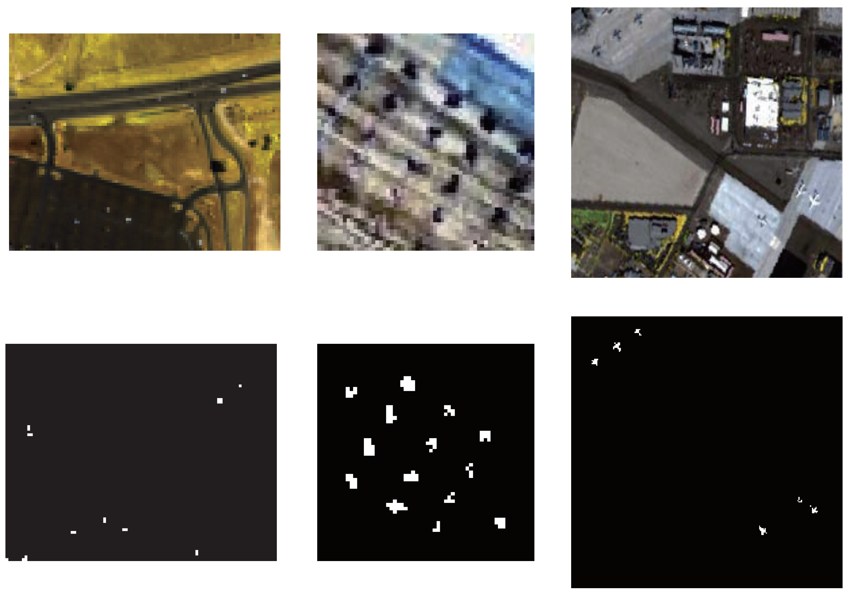
The first hyperspectral image is the HYDICE Urban data set. This real-world hyperspectral image is downloaded from the website of U.S. Army Engineer Research and Development Center (http://www.erdc.usace.army.mil/Media/FactSheets/FactSheetsArticleView/tabid/9254/Article/476681/hypercube). Its reflectance spectra are collected by HYDICE on an airborne platform, scanning an urban scene. It has the spectral resolution of 10 nm covering spectral range of 400–2500 nm, and the spatial resolution of 1 m. The size of the original hyperspectral image is . Since the ground truth for the whole scene is difficult to determine, a sub-image with pixels is cropped from the upper right region of the whole image. This sub-image contains several cars and roofs that are regarded as anomalies. Its corresponding ground truth is defined referring to the works [46,52]. The false color image and the ground truth map of this urban sub-image are shown in the first column of Figure 1. For the ground truth map, the highlighted pixels denote the locations of anomalies, and the black region is the background.
The remaining two real-world data sets are cropped from the different regions of the same hyperspectral image named AVIRIS which is acquired by the Airborne Visible/Infrared Imaging Spectrometer (AVIRIS) from San Diego, CA, USA. Its spectra range from 370 nm to 2510 nm with 224 spectral bands. Its spatial resolution is 3.5 m. Referring to the work [53], several spectral bands with the characteristics of either water absorption regions or low-SNR are removed, including 1–6, 33–35, 97, 107–113, 153–166, and 221–224. Therefore, totally 189 bands are used in the experiments. As for these two sub-images, one has the size of containing 14 planes regarded as abnormal targets in this scene; the other has the size of and there are 6 planes as anomalies. For simplicity, these two sub-images are named as AVIRIS1 and AVIRIS2 respectively in this work. The corresponding false color images and ground truth maps are sequentially shown in the second and third columns of Figure 1.
3.2. Experimental Details
In this section, the evaluation criterion, the employed competitors and parameter setup involved in the experiments are introduced in detail as follows.
3.2.1. Evaluation Criterion
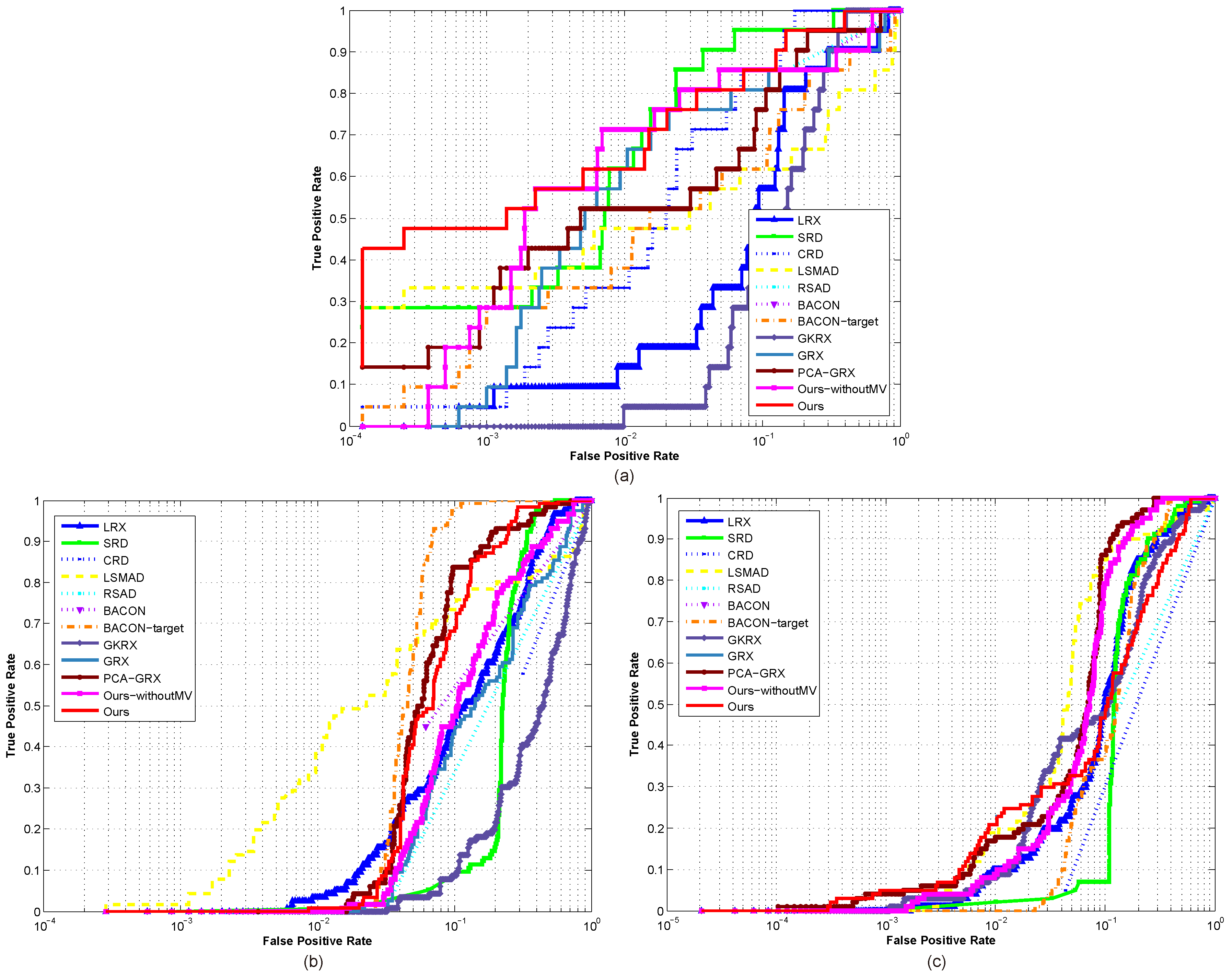
A valid evaluation criterion is very important to analyze and compare the performance of anomaly detectors fairly. In this paper, the classical receiver operating characteristic (ROC) curve and area under the curve (AUC) value are used to estimate the detection performance for both qualitative and quantitative analyses. The ROC curve is plotted by a set of points of the target detection rates and the false alarm rates. It can directly reflect the trade-off relationship between these two rates. When a discrimination threshold is given, the values of these pairs of two rates can be exactly computed. As for an accurate quantitative analysis, AUC value is further computed through integrating the area under the ROC curve, which can intuitively estimate the performance of the detector.
3.2.2. Competitors
In order to verify the performance of our proposed method, a number of state-of -the-art methods are used in the experiment. Totally ten different kinds of competitors, including local RX (LRX), SRD, CRD, LSMAD, RSAD, BACON, BACON-target, global KRX (GKRX), global RX (GRX) and PCA-GRX, are used by taking a comprehensive view of popularity, recency, and variety. In the field of hyperspectral anomaly detection, these comparison methods usually serve as competitors which can be regarded as the benchmark detectors. Therefore, the performance estimation for a new anomaly detection method is more accurate and convincing when compared with them.
Specifically, LRX and GRX are two versions of the classical Reed-Xiaoli method. SRD, CRD, and LSMAD are some sparse representation based methods. RSAD and BACON [54] are two novel anomaly detection methods with the aim of obtaining an accurate background estimation by taking away the potential anomalies. Since the proposed method utilizes some knowledge of anomalies, we also compare with the BACON-target [55] method which further takes the abnormal target information into consideration after applying the BACON method in order to reduce its false alarm rate. We compare with the global KRX method by mapping the original feature into the high dimensional feature space as well. Moreover, in order to demonstrate the effectiveness of our multiple-dictionary sparse feature extraction, the traditional PCA [56] method is used to reduce the spectral dimensions before implementing the GRX method, denoted as PCA-GRX. In addition, we also design another verification experiment to evaluate the superiority of the proposed global multiple-view anomaly detection strategy. After selecting different groups of representative features corresponding to multiple dictionaries, we directly concatenate all the features to generate one new hyperspectral data set and apply GRX to finish anomaly detection, named as Ours-withoutMV. Besides, it is noteworthy that since we use the simple and fast GRX method as the preliminary method, therefore, the whole performance of the proposed method can be demonstrated when compared with GRX.
3.2.3. Parameter Setup
In this part, some important parameters will be set. For the proposed method, four main parameters including the size of dictionary N, the number of clusters K, the regularized parameter , and the feature selection ratio are elaborated as follows. The value of N is determined mainly depending on the number of anomaly pixels detected by an simple preliminary detection. Since the pixel whose detection probability is larger than a given threshold will be regarded as an anomaly, in fact N is closely related to the threshold value. In our paper, considering that anomaly usually has a low occurrence probability, a value corresponding to the percentile of all the initial detection probabilities is empirically set as the threshold. The value of K determines the scale of multiple dictionaries reflecting the different attributes of background. It will take different values in accordance with the scale and scene complexity of a hyperspectral image. As for , deciding the number of the selected features, it closely relates to the contained materials as well. We carry out a deep analysis about parameter selection rules including K, and in Section 3.5. Here, we just claim the final assigned vale to each parameter in the comparison experiment respectively. For Urban, AVIRIS1, and AVIRIS2, the values of K are set as 10, 5 and 2; is completely fixed at 10; the values of are , , and in turn. The parameters for Ours-withoutMV is consistent in the camparison experiment.
Since some of the state-of-the-art competitors, such as LRX, SRD and CRD, use the sliding window technique, the window sizes containing both outside window and inner window should be claimed. Generally, different hyperspectral images have various abnormal targets with different sizes, and different competitors often require different appropriate window sizes. Therefore, in order to compare fairly, we set many different pairs of window sizes for these three detectors. We set two kinds of inner window sizes including and according to the targets’ possible largest size. For LRX method, in order to avoid covariance matrix singular problem, we finally use four pairs of window sizes including , , , and by comprehensively considering all the spectral dimensions of all the hyperspectral images. As for SRD and CRD, we define six kinds of different sizes including , , , , , and . In addition, the regularized parameter involved in CRD method is set as referring to its original work [45]. The parameters of LSMAD are strictly kept consistent with its original work [41]. We fix the maximal rank of the background matrix r at 2, and sparse cardinality k at . As for RSAD, the size of the randomly selected image block is fixed at 70. For BACON, the integer c is set as 4 according to its original work. The parameters involved in BACON-target are also consistent with its original literature. We set , and first 15 principal component images are acquired. As for GKRX, according to [33], the width of the Gaussian RBF kernel is fixed at 40, and the number of cluster centers is set as 600. The number of spectral dimensions is empirically reduced to 10 in PCA-GRX.
3.3. Comparison Results
In this section, the performance of our proposed algorithm is evaluated and analyzed through comparing with all the competitors. The experimental results are thoroughly and meticulously discussed according to qualitative and quantitative comparisons. Considering the simplicity of typesetting, for LRX, SRD and CRD, we only present the visualization pictures and ROC curves of their best results on the corresponding optimal window sizes, which are underlined in Table 1. AUC values and time consumption on all different window sizes are shown in Table 1 and Table 2 respectively. For all the competitors, the highest three results are remarked in bold. The average performance of AUC values and time consumption of all the competitors on the three data sets is illustrated in Table 3.
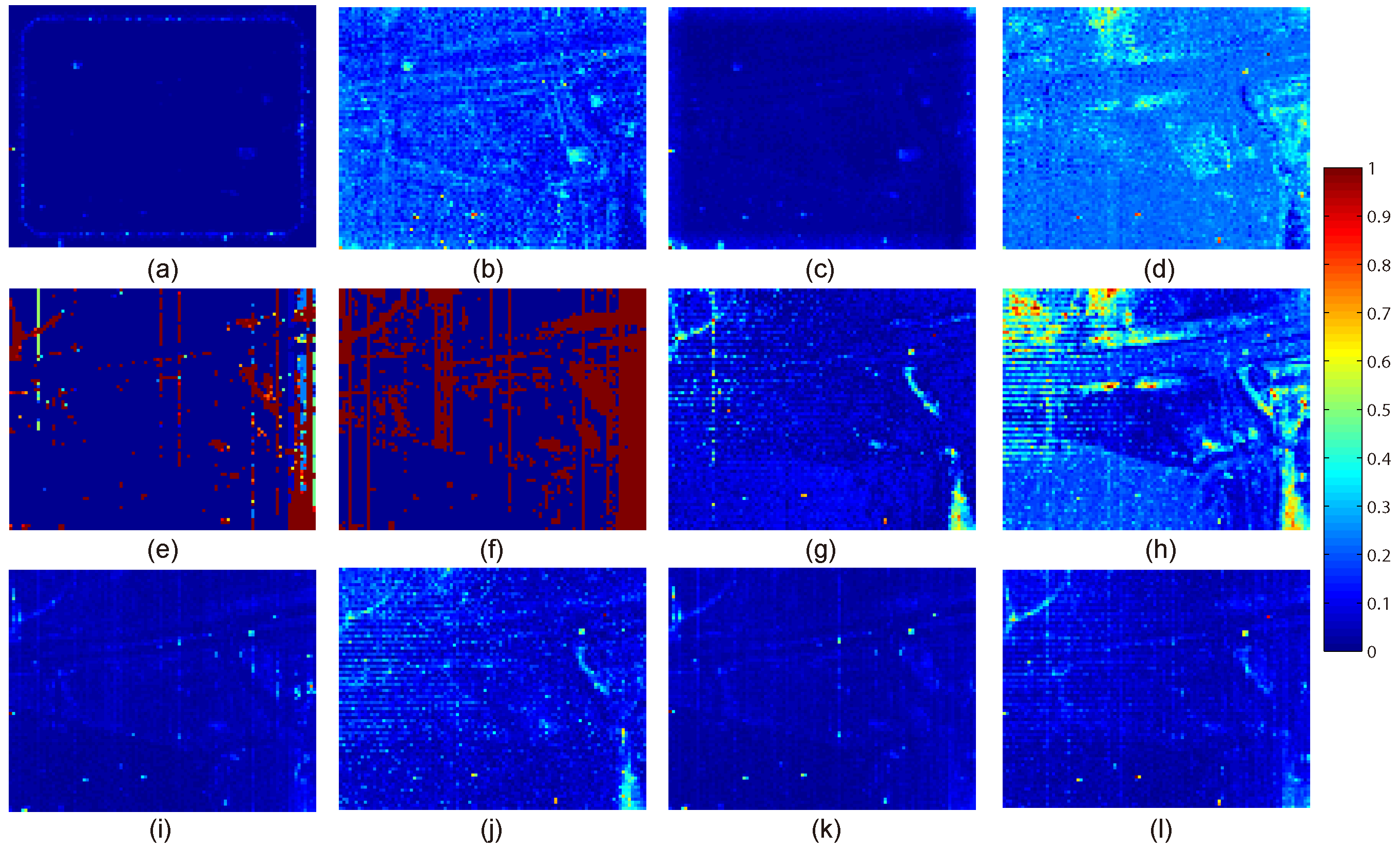
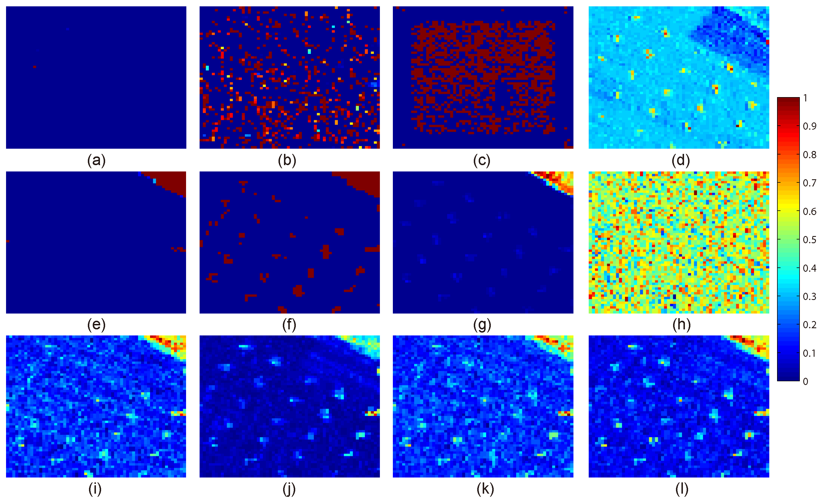
The visualization results on the HYDICE Urban hyperspectral image are presented in Figure 2. It can be obviously seen that RSAD and BACON have a very high false alarm rate. GKRX also seems to assign relatively salient intensities for some background regions. LRX, LSMAD and BACON-target have some omissions and many obvious false alarms. As for the rest competitors, their visualization results are similar for they can nearly recognize all of the abnormal targets. The main result difference of these competitors is the different intensities assigned to background and targets. The background clutter of SRD is obvious. The anomalies detected by CRD are not salient compared with the background. Taking both the ability to recognize anomalies and the ability to suppress background clutter through analyzing all the visualization results, the proposed method shows the best performance. In order to evaluate the performance fairly, ROC curves and AUC values are further compared. As it is shown in Figure 3a, on the whole, the ROC curve of the proposed method is obviously above all the curves of other benchmark competitors except for SRD and Ours-withoutMV almost in the whole false alarm rate range. Compared with SRD, our method shows its significant superiority of keeping getting the highest detection rates when the false alarm rates are in the range of even less than . Our method has higher detection rate than all the other competitors even in the case of requiring a very low false alarm rate. This phenomenon proves the superior distinctiveness of the selected spectral features by the proposed method. Compared with Ours-withoutMV, the similar result demonstrates the effectiveness of our global multiple-view anomaly detection strategy. When considering the AUC values shown in Table 1, the proposed method also achieves a promising result for its value is only slightly less than those of SRD and CRD, while is greatly larger than the rest of competitors. However, it can be seen that SRD and CRD seem sensitive to the window sizes as shown in Table 1. Therefore, to conclude, all of these results fully confirm the effectiveness of the proposed method. It has a better ability to describe the difference between background and anomaly, and the good advantage of recognizing different kinds of targets.
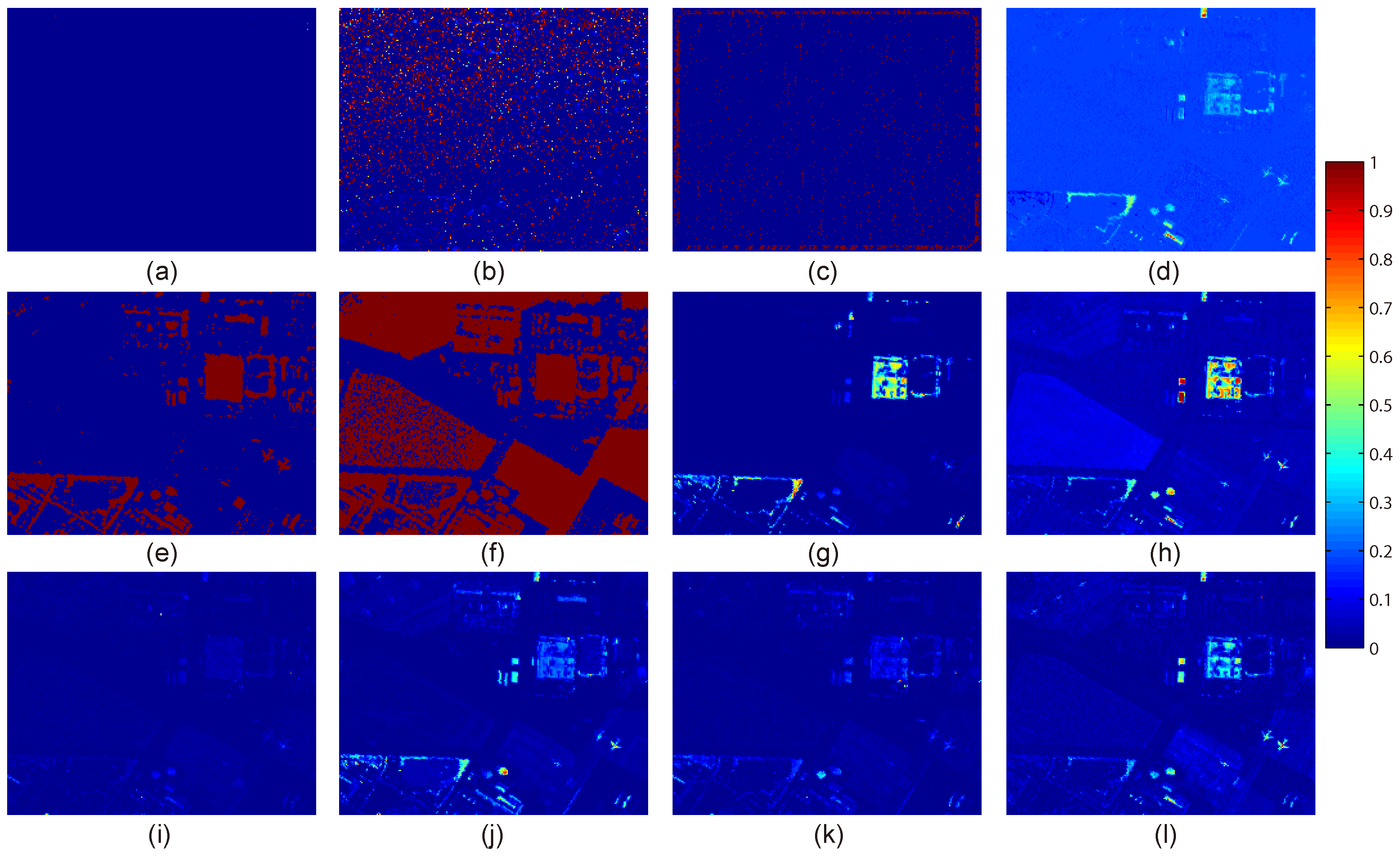
The AVIRIS1 data set has lots of anomalies and all of them are with a relative large size. Thus the effect of anomalies on the estimation of background is hard to avoid. From Figure 4, it can be seen that SRD, CRD, RSAD and BACON have a serious problem of high false alarm rate. RSAD nearly fails to detect all the targets and conversely assigns very high anomaly probabilities to some background. Although BACON can detect the abnormal targets, it also recognizes some background regions as anomalies. The performance of LRX is poor for it can just detect a few abnormal pixels. The reason behind is that abnormal targets’ effect on the estimation of background is exceedingly serious in each local sliding window. The GKRX also fails to detect anomalies. LSMAD has better performance than the previously-mentioned methods for it can distinctly detect many anomaly targets. However, its background suppression is not satisfactory. For the other methods, the detection results are similar to a certain extent. Compared with GRX and Ours-withoutMV, BACON-target, PCA-GRX and our proposed method are better because they seem to succeed in suppressing the background. The ROC curves and AUC values are further analyzed for an accurate estimation. Figure 3b plots the ROC curves of all the detectors on this hyperspectral image. It can be seen that the proposed method obtains far superior ROC curve to most of the competitors. Although LSMAD can obtain the best performance when the detection rate is less than about , its false alarms are very serious when it gets the detection rate. However, the BACON-target, PCA-GRX and our method can quickly achieve the highest detect rate at a relatively lower false alarm rate. For the AUC quantitative comparison shown in Table 1, the proposed method obtains the higher value with significant superiority. Although, our method does not obtain the best result on this data set, it is still in the top three. Moreover, our method has made a dramatic improvement to the original GRX method, which directly verifies its entire effectiveness of our two important motivations. The significant performance improvement compared with Ours-withoutMV also demonstrates the good virtue of global multiple-view anomaly detection strategy. In summary, our method has shown its good ability to suppress the background and detect anomalies.
The visualization comparison results on the AVIRIS2 data set are presented in Figure 5. It can be obviously seen that RSAD and BACON have a serious problem of high false alarm rate. SRD and CRD also assign high intensities to many background pixels. The performance of LRX is inferior for it seems to hardly detect a few of targets for the visual inspection. GRX seems much better than the above mentioned methods for it can detect more targets. LSMAD shows its good ability to detect anomalies but it still has unsatisfactory ability to suppress background clutter. As for the remaining competitors, their detection results are similar as a whole and the main difference exists in some local regions with different salience. Fortunately, the performance of the proposed method seems better than others because it can not only detect almost all the abnormal targets, but also assign each target a remarkable detection probability. Moreover, the background is also suppressed obviously. Figure 3c illustrates the ROC curves of all the detectors, and the corresponding AUC values are shown in Table 1. The proposed method completely defeats all the other competitors. It obtains the highest detection rate when the false alarm rate is in the range of approximately less than . Our method also obtains the highest AUC value, a totally satisfactory detection result, making a dramatic improvement compared with some competitors whose AUC values are really low. In addition, our method’s better performance than PCA-GRX verifies the good virtue of multiple-dictionary sparse feature extraction strategy; its superior result to Ours-withoutMV demonstrates the effectiveness of global multiple-view anomaly detection strategy. Therefore, through the above results and analyses, the superiority of our method has been demonstrated. Owing to the representative feature selection technique, the difference between background and anomaly has been enhanced. The proposed method can successfully distinguish anomalies from the background. Besides, taking good advantage of its global multiple-view operator, all different sizes of targets can be well detected and the detection performance is excellent.
On the whole, compared with the ten state-of-the-art competitors, our method shows its superiority in detecting different abnormal targets and suppressing the background, which convincingly verifies the good distinctiveness of the selected representative features that enlarge the difference between anomalies and background. Overall, although our method does not keeps getting the best results on all the data sets, its comprehensive performance has always been in the top three, which is significantly better than some methods may only performing well occasionally on one data set. The average performance of each method on all the data sets is shown in Table 3, in which the average values of LRX, SRD and CRD are obtained according to their best results on each data. Our method gets the highest average AUC, which also demonstrates its excellent and stable performance. Besides, according to result analysis on each data set, the effectiveness of the proposed two important procedures are objectively proved compared with PCA-GRX, GRX, and Ours-withoutMV.
3.4. Comparison of Time Consumption
The time consumption of all the detectors employed in this work is discussed in this part. All the methods are implemented on a machine with Intel Core i3-2130 3.4-GHz CPU and 16-GB RAM in the MATLAB R2012b platform under the Windows 7 64-bit operating system. The time consumption of each method in the unit of second is illustrated in Table 2. Comprehensively all the results, PCA-GRX is the fastest method almost on all the data sets. Benefiting from the global processing, GRX also shows excellent efficiency for it only takes slightly more running time than PCA-GRX. Following GRX, the whole time consumption of BACON and our method is relatively close and efficient according to the complete analysis on the three data sets. The performance of BACON-target is not stable, because although it shows its good efficiency on the first two data sets, however, it suffers the unacceptable time burden on the last image. As for LRX, SRD, CRD, LSMAD, RSAD, and GKRX, they have much heavier time consumption than GRX by more than one or two orders of magnitude. Moreover, for LRX, SRD and CRD, their running time is increasing sharply with the change of window size and image size, and the LRX has the heaviest time consumption. On the whole, compared with the all the other competitors, our method shows its good performance on efficiency because its time consumption is obviously less than most of the competitors except for PCA-GRX and GRX. Since we take GRX method as our preprocessing procedure, it understandably takes more time than GRX. Fortunately, its running time is just slightly higher than that of GRX on each data set, which demonstrates the proposed multiple-dictionary sparse feature extraction technique dose not cause much more time consumption. The average time consumption of each competitor on all the three data sets shown in Table 3 also demonstrates the good performance of our method in efficiency. To sum up, the proposed method is efficient within a promising and reasonable time cost range.
3.5. Parameters Setting Discussion
In this part, we will analyze the effects of different parameters on the detection performance, and discuss the parameter setting criteria. There are three important parameters involved in the proposed method including the number of clusters K, the regularized parameter , and the feature selection ratio . In order to have a more convincing discussion, the parameter experiments are conducted respectively on each hyperspectral image.
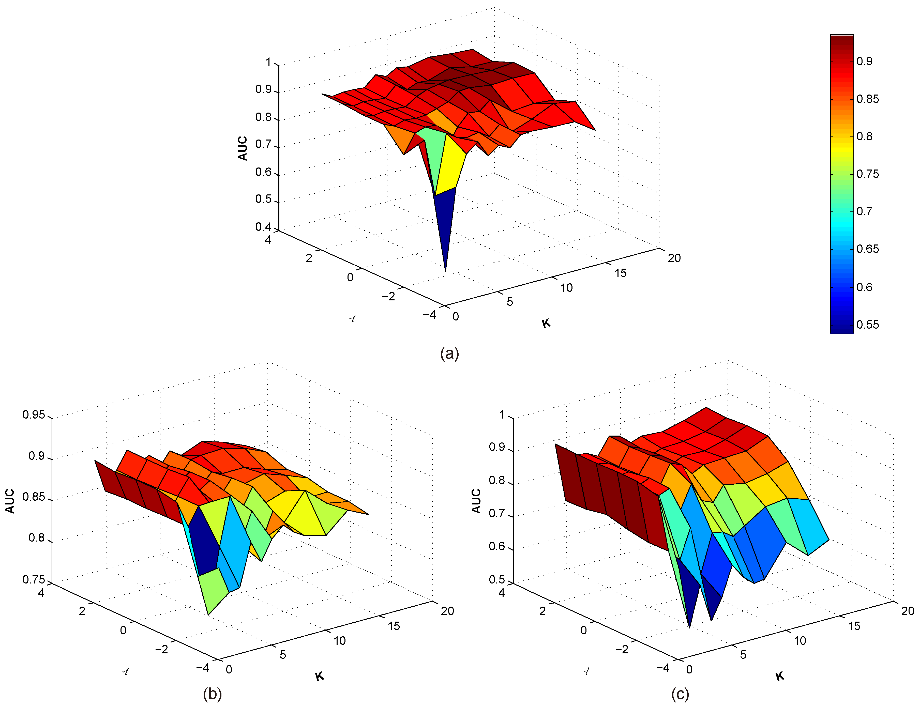
For simplicity, we first simultaneously analyze the effects of the number of clusters K and the regularized parameter on the Urban, AVIRIS1, and AVIRIS2. K is successively chosen from the set of , and is chosen from , while the other parameters are fixed. The experimental results are shown in Figure 6. It should be noted that the coordinate value corresponding to takes the logarithms (base 10) of parameters. From Figure 6, through comprehensively analyzing all the results of the three hyperspectral images, it can be seen that with the increasing of , the detection performance is firstly significantly improved to reach a promising result, and then nearly maintains a higher AUC value within a slightly floating change. On the whole, when the value of is equal or greater than 1, the proposed method can get a satisfactory result. As for parameter K, it can be seen that the number of clusters does not have a very obvious effect on the detection performance. In other words, our method is not very sensitive to the variation of K. Considering the convenience in the practical implementation of our method, we suggest that the number of clusters K can be selected in accordance with the scene complexity of a hyperspectral image. If the image is complex containing many different kinds of materials, K can be assigned a relatively larger value. If the image scene seems simple, K will be set as a smaller value.
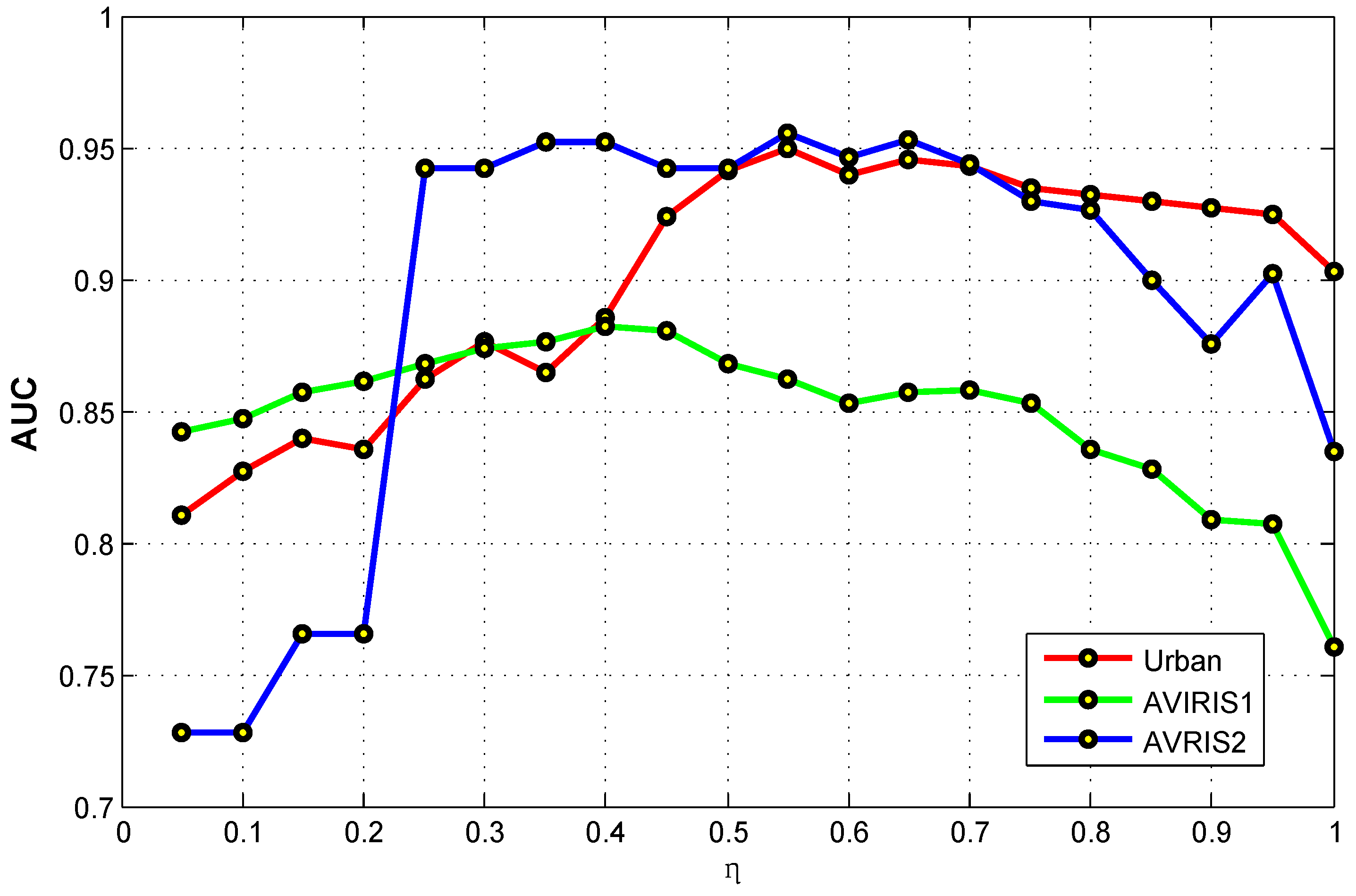
Then we discuss the effect of the feature selection ratio on the detection performance. The parameter is changed from to 1 at the interval of for all the three hyperspectral images. The value 1 means that all the original bands are picked out after conducting the feature selection process. The experimental results are plotted on Figure 7. All the result curves of the hyperspectral images reflect the fact that the feature selection is really effective and imperative because the AUC values corresponding to most of the ratios are higher than the AUC value of ratio 1. Nevertheless, there also exist some special cases that improper feature selections will even reduce the detection performance. The main reason behind is when the ratio is too small, a certain very small number of spectral bands may be picked out. Consequently, the selected features seem insufficient to describe the characteristics of different materials. As a result, it is difficult to further distinguish anomalies from different background materials. On the whole, according to the experimental result, the detection performance is relatively sensitive to the feature selection ratio. However, this parameter sensitiveness problem is not specific to our method, which is still an open problem in the field of feature selection.
4. Conclusions
This paper proposes a novel hyperspectral anomaly detection method by designing a multiple-dictionary sparse feature extraction approach. Considering that the characteristics of the high spectral dimension and complicated spectral correlation have negative effects on the performance of anomaly detection, therefore, an effective feature selection is really necessary to address this problem in order to improve the detection performance. Different from directly and simply applying the feature selection method to anomaly detection task, we design a novel feature selection technique which is closely guided by anomaly detection. In order to select the discriminative features, the background and the anomaly information obtained from an preliminary detection operator is jointly used to construct the sparse dictionary representation process. Through this way, these representative features which can significantly enhance the difference between background spectra and anomaly spectra will be selected. Taking the background complexity into consideration, multiple dictionaries are constructed in order to accurately characterize the various attributes of different material clusters. Finally, the global multiple-view anomaly detection strategy is used to obtain an accurate detection result by completely considering all the decision-making abilities of different groups of the selected features specific to different background categories. In order to demonstrate the good performance of the proposed method, ten state-of-the-art competitors are used for a fair and convincing comparison. All the methods are implemented on three real-word hyperspectral images. Extensive experimental results show that the proposed method is superior to all the other competitors after comprehensively evaluating the effectiveness and efficiency. Compared with LRX, SRD, CRD, LSMAD, RSAD, BACON, BACON-target, GKRX, GRX, and PCA-GRX, the proposed method has the obvious improvement of about , , , , , , , , , and respectively according to the average AUC results on all the data sets. Its average time consumption less than 10 s also shows its promising application value. Benefiting from the good virtues of feature selection technique and the global multiple-view anomaly detection strategy, our method can not only have good ability to detect different targets with different sizes, but also have an obvious success in background suppression. The selected discriminative features can significantly enhance the distinctiveness to recognize anomalies from background, and the multiple-view strategy can comprehensively take full use of all the estimation abilities corresponding to different background characteristics. Therefore, the proposed method can obtain excellent performance. Considering that the spatial characteristic also plays an important role in analyzing different materials, we will apply this information in the proposed feature selection approach in our future work.
Author Contributions
All authors made contributions to proposing the method, performing the experiments and analyzing the results. All authors contributed to the perparation and revison of the manuscript.
Acknowledgments
This work was supported by the National Key R&D Program of China under Grant 2017YFB1002202, State Key Program of National Natural Science of China under Grant 60632018, National Natural Science Foundation of China under Grant 61773316, Fundamental Research Funds for the Central Universities under Grant 3102017AX010, and the Open Research Fund of Key Laboratory of Spectral Imaging Technology, Chinese Academy of Sciences.
Conflicts of Interest
The authors declare no conflict of interest.
References
- Zhu, L.; Wen, G. Hyperspectral anomaly detection via background estimation and adaptive weighted sparse representation. Remote Sens. 2018, 10, 272. [Google Scholar]
- Zhao, L.; Lin, W.; Wang, Y.; Li, X. Recursive local summation of rx detection for hyperspectral image using sliding windows. Remote Sens. 2018, 10, 103. [Google Scholar] [CrossRef]
- Wang, Q.; Lin, J.; Yuan, Y. Salient band selection for hyperspectral image classification via manifold ranking. IEEE Trans. Neural Netw. Learn. Syst. 2016, 27, 1279–1289. [Google Scholar] [CrossRef] [PubMed]
- Wang, Q.; Gao, J.; Yuan, Y. A Joint convolutional neural networks and context transfer for street scenes labeling. IEEE Trans. Intell. Transp. Syst. 2017, 19, 1457–1470. [Google Scholar] [CrossRef]
- Alarcon-Ramirez, A.; Rwebangira, M.; Chouikha, M.; Manian, V. A new methodology based on level sets for target detection in hyperspectral images. IEEE Trans. Geosci. Remote Sens. 2016, 54, 5385–5396. [Google Scholar] [CrossRef]
- Zhang, Y.; Wu, K.; Du, B.; Zhang, L.; Hu, X. Hyperspectral target detection via adaptive joint sparse representation and multi-task learning with locality information. Remote Sens. 2017, 9, 482. [Google Scholar] [CrossRef]
- He, Z.; Wang, Y.; Hu, J. Joint sparse and low-rank multitask learning with laplacian-like regularization for hyperspectral classification. Remote Sens. 2018, 10, 322. [Google Scholar] [CrossRef]
- Gao, L.; Zhao, B.; Jia, X.; Liao, W.; Zhang, B. Optimized kernel minimum noise fraction transformation for hyperspectral image classification. Remote Sens. 2017, 9, 548. [Google Scholar] [CrossRef]
- Liu, K.; Chen, S.; Chien, H.; Lu, M. Progressive sample processing of band selection for hyperspectral image transmission. Remote Sens. 2018, 10, 367. [Google Scholar] [CrossRef]
- Yuan, Y.; Lin, J.; Wang, Q. Dual-clustering-based hyperspectral band selection by contextual analysis. IEEE Trans. Geosci. Remote Sens. 2016, 54, 1431–1445. [Google Scholar] [CrossRef]
- Zhang, X.; Li, C.; Zhang, J.; Chen, Q.; Feng, J.; Jiao, L.; Zhou, H. Hyperspectral unmixing via low-rank representation with space consistency constraint and spectral library pruning. Remote Sens. 2018, 10, 339. [Google Scholar] [CrossRef]
- Rizkinia, M.; Okuda, M. Joint local abundance sparse unmixing for hyperspectral images. Remote Sens. 2017, 12, 1224. [Google Scholar] [CrossRef]
- Nasrabadi, N. Hyperspectral target detection: An overview of current and future challenges. IEEE Signal Process. Mag. 2014, 31, 34–44. [Google Scholar] [CrossRef]
- Wang, Q.; Meng, Z.; Li, X. Locality adaptive discriminant analysis for spectral-spatial classification of hyperspectral images. IEEE Geosci. Remote Sens. Lett. 2017, 14, 2077–2081. [Google Scholar] [CrossRef]
- Wang, Q.; Wan, J.; Yuan, Y. Locality constraint distance metric learning for traffic congestion detection. Pattern Recognit. 2018, 75, 272–281. [Google Scholar] [CrossRef]
- Wang, Q.; Gao, J.; Yuan, Y. Embedding structured contour and location prior in siamesed fully convolutional networks for road detection. IEEE Trans. Intell. Transp. Syst. 2018, 19, 230–241. [Google Scholar] [CrossRef]
- Gevaert, C.; Suomalainen, J.; Tang, J.; Kooistra, L. Generation of spectral-temporal response surfaces by combining multispectral satellite and hyperspectral uav imagery for precision agriculture applications. IEEE J. Sel. Top. Appl. Earth Obs. Remote Sens. 2015, 8, 3140–3146. [Google Scholar] [CrossRef]
- Kruse, F.; Boardman, J.; Huntington, J. Comparison of airborne hyperspectral data and eo-1 hyperion for mineral mapping. IEEE Trans. Geosci. Remote Sens. 2003, 41, 1388–1400. [Google Scholar] [CrossRef]
- Taghipour, A.; Ghassemian, H. Hyperspectral anomaly detection using attribute profiles. IEEE Geosci. Remote Sens. Lett. 2017, 14, 1136–1140. [Google Scholar] [CrossRef]
- Wang, Q.; Wan, J.; Yuan, Y. Deep metric learning for crowdedness regressiong. IEEE Trans. Circuits Syst. Video Technol. 2017. [Google Scholar] [CrossRef]
- Matteoli, S.; Acito, N.; Diani, M.; Corsini, G. An automatic approach to adaptive local background estimation and suppression in hyperspectral target detection. IEEE Trans. Geosci. Remote Sens. 2011, 49, 790–800. [Google Scholar] [CrossRef]
- Kwon, H.; Nasrabadi, N.M. Kernel matched subspace detectors for hyperspectral target detection. IEEE Trans. Pattern Anal. Mach. Intell. 2006, 28, 178–194. [Google Scholar] [CrossRef] [PubMed]
- Khazai, S.; Safari, A.; Mojaradi, B.; Homayouni, S. An approach for subpixel anomaly detection in hyperspectral images. IEEE J. Sel. Top. Appl. Earth Obs. Remote Sens. 2013, 6, 769–778. [Google Scholar] [CrossRef]
- Matteoli, S.; Diani, M.; Corsini, G. A tutorial overview of anomaly detection in hyperspectral images. IEEE Trans. Aerosp. Electron. Syst. 2010, 25, 5–28. [Google Scholar] [CrossRef]
- Sun, W.; Tian, L.; Xu, Y.; Du, B.; Du, Q. A randomized subspace learning based anomaly detector for hyperspectral imagery. Remote Sens. 2018, 10, 417. [Google Scholar] [CrossRef]
- Reed, I.; Yu, X. Adaptive multiple-band CFAR detection of an optical pattern with unknown spectral distribution. IEEE Trans. Acoust. Speech Sign. Proc. 1990, 38, 1760–1770. [Google Scholar] [CrossRef]
- Imani, M. RX anomaly detector with rectified background. IEEE Geosci. Remote Sens. Lett. 2017, 14, 1313–1317. [Google Scholar] [CrossRef]
- Li, W.; Wu, G.; Du, Q. Transferred deep learning for anomaly detection in hyperspectral imagery. IEEE Geosci. Remote Sens. Lett. 2017, 14, 597–601. [Google Scholar] [CrossRef]
- Yuan, Y.; Ma, D.; Wang, Q. Hyperspectral anomaly detection by graph pixel selection. IEEE Trans. Cybern. 2016, 46, 3123–3134. [Google Scholar] [CrossRef] [PubMed]
- Soofbaf, S.; Sahebi, M.; Mojaradi, B. A sliding window-based joint sparse representation (swjsr) method for hyperspectral anomaly detection. Remote Sens. 2018, 10, 434. [Google Scholar] [CrossRef]
- Du, B.; Zhang, L. Random-selection-based anomaly detector for hyperspectral imagery. IEEE Trans. Geosci. Remote Sens. 2011, 49, 1578–1589. [Google Scholar] [CrossRef]
- Zhao, R.; Du, B.; Zhang, L. A robust nonlinear hyperspectral anomaly detection approach. IEEE J. Sel. Top. Appl. Earth Obs. Remote Sens. 2014, 7, 1227–1234. [Google Scholar] [CrossRef]
- Kwon, H.; Nasrabadi, N.M. Kernel rx-algorithm: A nonlinear anomaly detector for hyperspectral imagery. IEEE Trans. Geosci. Remote Sens. 2005, 43, 388–397. [Google Scholar] [CrossRef]
- Banerjee, A.; Burlina, P.; Diehl, C. A support vector method for anomaly detection in hyperspectral imagery. IEEE Trans. Geosci. Remote Sens. 2006, 44, 2282–2291. [Google Scholar] [CrossRef]
- Zhou, J.; Kwan, C.; Ayhan, B.; Eismann, M.T. A novel cluster kernel rx algorithm for anomaly and change detection using hyperspectral images. IEEE Trans. Geosci. Remote Sens. 2016, 54, 6497–6504. [Google Scholar] [CrossRef]
- Carlotto, M.J. A cluster-based approach for detecting man-made objects and changes in imagery. IEEE Trans. Geosci. Remote Sens. 2005, 43, 374–387. [Google Scholar] [CrossRef]
- Xu, Y.; Wu, Z.; Li, J.; Plaza, A.; Wei, Z. Anomaly detection in hyperspectral images based on low-rank and sparse representation. IEEE Trans. Geosci. Remote Sens. 2016, 54, 1990–2000. [Google Scholar] [CrossRef]
- Yuan, Z.; Sun, H.; Ji, K.; Li, Z.; Zou, H. Local sparsity divergence for hyperspectral anomaly detection. IEEE Geosci. Remote Sens. Lett. 2014, 11, 1697–1701. [Google Scholar] [CrossRef]
- Qu, Y.; Guo, R.; Wang, W.; Qi, H.; Ayhan, B.; Kwan, C.; Vance, S. Anomaly detection in hyperspectral images through spectral unmixing and low rank decomposition. In Proceedings of the 2016 IEEE International Geoscience and Remote Sensing Symposium, Beijing, China, 10–15 July 2016; pp. 1855–1858. [Google Scholar]
- Wang, W.; Li, S.; Qi, H.; Ayhan, B.; Kwan, C.; Vance, S. Identify anomaly component by sparsity and low rank. In Proceedings of the 2015 7th Workshop on Hyperspectral Image and Signal Processing: Evolution in Remote Sensing, Tokyo, Japan, 2–5 June 2015; pp. 1–4. [Google Scholar]
- Zhang, Y.; Du, B.; Zhang, L.; Wang, S. A low-rank and sparse matrix decomposition-based mahalanobis distance method for hyperspectral anomaly detection. IEEE Trans. Geosci. Remote Sens. 2016, 54, 1376–1389. [Google Scholar] [CrossRef]
- Niu, Y.; Wang, B. Hyperspectral anomaly detection based on low-rank representation and learned dictionary. Remote Sens. 2016, 8, 289. [Google Scholar] [CrossRef]
- Li, J.; Zhang, H.; Ma, L. Hyperspectral anomaly detection by the use of background joint sparse representation. IEEE J. Sel. Top. Appl. Earth Obs. Remote Sens. 2015, 8, 2523–2533. [Google Scholar] [CrossRef]
- Zhang, Y.; Du, B.; Zhang, L.; Liu, T. Joint sparse representation and multitask learning for hyperspectral target detection. IEEE Trans. Geosci. Remote Sens. 2017, 55, 894–906. [Google Scholar] [CrossRef]
- Li, W.; Du, Q. Collaborative representation for hyperspectral anomaly detection. IEEE Trans. Geosci. Remote Sens. 2015, 53, 1463–1474. [Google Scholar] [CrossRef]
- Zhao, R.; Du, B.; Zhang, L. Hyperspectral anomaly detection via a sparsity score estimation framework. IEEE Trans. Geosci. Remote Sens. 2017, 55, 3208–3222. [Google Scholar] [CrossRef]
- Chen, Y.; Nasrabadi, N.; Tran, T. Hyperspectral image classification using dictionary-based sparse representation. IEEE Trans. Geosci. Remote Sens. 2011, 49, 3973–3985. [Google Scholar] [CrossRef]
- Dao, M.; Kwan, C.; Koperski, K.; Marchisio, G. A joint sparsity approach to tunnel activity monitoring using high resolution satellite images. In Proceedings of the 2017 IEEE 8th Annual Ubiquitous Computing, Electronics and Mobile Communication Conference, New York, NY, USA, 19–21 October 2017; pp. 322–328. [Google Scholar]
- Yuan, Y.; Zheng, X.; Lu, X. Discovering diverse subset for unsupervised hyperspectral band selection. IEEE Trans. Image Process. 2017, 26, 51–64. [Google Scholar] [CrossRef] [PubMed]
- Arthur, D.; Vassilvitskii, S. K-means++: The advantages of careful seeding. In Proceedings of the 18th annual ACM-SIAM symposium on Discrete algorithms, New Orleans, LA, USA, 7–9 January 2007; pp. 1027–1035. [Google Scholar]
- Li, X.; Lu, Q.; Dong, Y.; Tao, D. SCE: A manifold regularized set-covering method for data partitioning. IEEE Trans. Neural Netw. Learn. Syst. 2017, 29, 1760–1773. [Google Scholar] [CrossRef] [PubMed]
- Ma, D.; Yuan, Y.; Wang, Q. A sparse dictionary learning method for hyperspectral anomaly Detection with capped norm. In Proceedings of the 2017 IEEE International Geoscience and Remote Sensing Symposium, Fort Worth, TX, USA, 23–28 July 2017; pp. 648–651. [Google Scholar]
- Du, B.; Zhang, Y.; Zhang, L.; Tao, D. Beyond the sparsity-based target detector: A hybrid sparsity and statistics-based detector for hyperspectral images. IEEE Trans. Image Process. 2016, 25, 5345–5357. [Google Scholar] [CrossRef] [PubMed]
- Billora, N.; Hadib, A.; Velleman, P. BACON: Blocked adaptive computationally efficient outlier nominators. Comput. Stat. Data Anal. 2000, 34, 279–298. [Google Scholar] [CrossRef]
- Guo, Q.; Pu, R.; Gao, L.; Zhang, B. A novel anomaly detection method incorporating target information derived from hyperspectral imagery. IEEE Geosci. Remote Sens. Lett. 2015, 7, 11–20. [Google Scholar] [CrossRef]
- Eismann, T.; Meola, J.; Hardie, R. Hyperspectral change detection in the presence of diurnal and seasonal variations. IEEE Trans. Geosci. Remote Sens. 2008, 46, 237–249. [Google Scholar] [CrossRef]
Figure 1.
The visualization of the HSIs and the ground truth maps. The first row shows the false color pictures of Urban data set, AVIRIS1 data set, and AVIRIS2 data set respectively. The second row illustrates their corresponding ground truth maps.
Figure 1.
The visualization of the HSIs and the ground truth maps. The first row shows the false color pictures of Urban data set, AVIRIS1 data set, and AVIRIS2 data set respectively. The second row illustrates their corresponding ground truth maps.

Figure 2.
The visualization results of different detectors on Urban data set. (a) LRX: window size (19,7); (b) SRD: window size (13,7); (c) CRD: window size (13,7); (d) LSMAD; (e) RSAD; (f) BACON; (g) BACON-target; (h) GKRX; (i) GRX; (j) PCA-GRX; (k) Ours-withoutMV; (l) Ours. Values in the color bar represent the anomaly probability.

Figure 3.
The ROC curves of different detectors on three hyperspectral images. (a) Urban data set; (b) AVIRIS1 data set; (c) AVIRIS2 data set.
Figure 3.
The ROC curves of different detectors on three hyperspectral images. (a) Urban data set; (b) AVIRIS1 data set; (c) AVIRIS2 data set.

Figure 4.
The visualization results of different detectors on AVIRIS1 data set. (a) LRX: window size (17,9); (b) SRD: window size (13,7); (c) CRD: window size (15,7); (d) LSMAD; (e) RSAD; (f) BACON; (g) BACON-target; (h) GKRX; (i) GRX; (j) PCA-GRX; (k) Ours-withoutMV; (l) Ours. Values in the color bar represent the anomaly probability.

Figure 5.
The visualization results of different detectors on AVIRIS2 data set. (a) LRX: window size (19,9); (b) SRD: window size (19,9); (c) CRD: window size (19,9); (d) LSMAD; (e) RSAD; (f) BACON; (g) BACON-target; (h) GKRX; (i) GRX; (j) PCA-GRX; (k) Ours-withoutMV; (l) Ours. Values in the color bar represent the anomaly probability.

Figure 6.
The experimental results of different settings of the number of clusters K and the regularized parameter on three hyperspectral images. (a) Urban data set; (b) AVIRIS1 data set; (c) AVIRIS2 data set. Values in the color bar represent the anomaly probability.
Figure 6.
The experimental results of different settings of the number of clusters K and the regularized parameter on three hyperspectral images. (a) Urban data set; (b) AVIRIS1 data set; (c) AVIRIS2 data set. Values in the color bar represent the anomaly probability.

Figure 7.
The effects of the feature selection ratio of the proposed method on three hyperspectral images including Urban data set, AVIRIS1data set, and AVIRIS2 data set.
Figure 7.
The effects of the feature selection ratio of the proposed method on three hyperspectral images including Urban data set, AVIRIS1data set, and AVIRIS2 data set.


Table 1.
AUC values of all the competitors on three hyperspectral images including Urban data set, AVIRIS1data set, and AVIRIS2 data set. The bold numbers represent the highest three results, and the underline marks the result under the optimal window size.
Table 1.
AUC values of all the competitors on three hyperspectral images including Urban data set, AVIRIS1data set, and AVIRIS2 data set. The bold numbers represent the highest three results, and the underline marks the result under the optimal window size.
| AUC | Urban | AVIRIS1 | AVIRIS2 | |
|---|---|---|---|---|
| LRX | (17,7) | 0.8184 | 0.5849 | 0.7627 |
| (17,9) | 0.7411 | 0.8104 | 0.6960 | |
| (19,7) | 0.8450 | 0.4843 | 0.8314 | |
| (19,9) | 0.8111 | 0.4516 | 0.8644 | |
| SRD | (13,7) | 0.9733 | 0.7809 | 0.8034 |
| (15,7) | 0.9243 | 0.7616 | 0.8093 | |
| (17,7) | 0.9037 | 0.7625 | 0.8112 | |
| (17,9) | 0.8902 | 0.7614 | 0.8400 | |
| (19,7) | 0.9118 | 0.7476 | 0.8152 | |
| (19,9) | 0.8997 | 0.7447 | 0.8425 | |
| CRD | (13,7) | 0.9609 | 0.4904 | 0.5013 |
| (15,7) | 0.9044 | 0.6288 | 0.4183 | |
| (17,7) | 0.4632 | 0.4515 | 0.4872 | |
| (17,9) | 0.7527 | 0.4639 | 0.4794 | |
| (19,7) | 0.5124 | 0.4663 | 0.4901 | |
| (19,9) | 0.5568 | 0.4521 | 0.5031 | |
| LSMAD | 0.7775 | 0.8329 | 0.9039 | |
| RSAD | 0.8749 | 0.4845 | 0.6717 | |
| BACON | 0.7895 | 0.6930 | 0.7327 | |
| BACON-target | 0.8515 | 0.9512 | 0.8608 | |
| GKRX | 0.8384 | 0.5523 | 0.8471 | |
| GRX | 0.9024 | 0.7601 | 0.8343 | |
| PCA-GRX | 0.9195 | 0.9084 | 0.9301 | |
| Ours-withoutMV | 0.9194 | 0.8250 | 0.9198 | |
| Ours | 0.9604 | 0.9052 | 0.9517 | |
Table 2.
Time consumption (seconds) of all the competitors on three hyperspectral images including Urban data set, AVIRIS1data set, and AVIRIS2 data set.
Table 2.
Time consumption (seconds) of all the competitors on three hyperspectral images including Urban data set, AVIRIS1data set, and AVIRIS2 data set.
| Time Consumption | Urban | AVIRIS1 | AVIRIS2 | |
|---|---|---|---|---|
| LRX | (17,7) | 126.52 | 54.21 | 756.45 |
| (17,9) | 122.39 | 62.93 | 915.49 | |
| (19,7) | 135.07 | 47.35 | 647.34 | |
| (19,9) | 126.67 | 67.01 | 958.67 | |
| SRD | (13,7) | 7.17 | 2.43 | 35.44 |
| (15,7) | 10.21 | 3.60 | 52.29 | |
| (17,7) | 13.50 | 4.80 | 67.89 | |
| (17,9) | 11.87 | 7.67 | 92.47 | |
| (19,7) | 17.21 | 5.79 | 94.21 | |
| (19,9) | 13.74 | 9.21 | 119.14 | |
| CRD | (13,7) | 14.47 | 6.913 | 99.47 |
| (15,7) | 23.82 | 11.64 | 178.60 | |
| (17,7) | 48.31 | 22.87 | 404.53 | |
| (17,9) | 36.27 | 22.44 | 344.06 | |
| (19,7) | 80.70 | 41.11 | 616.60 | |
| (19,9) | 61.13 | 36.97 | 617.99 | |
| LSMAD | 17.51 | 9.59 | 127.27 | |
| RSAD | 34.50 | 10.33 | 183.31 | |
| BACON | 3.91 | 1.41 | 22.92 | |
| BACON-target | 3.25 | 0.71 | 1533.62 | |
| GKRX | 65.00 | 41.01 | 76.22 | |
| GRX | 0.97 | 0.28 | 4.12 | |
| PCA-GRX | 0.65 | 0.30 | 3.62 | |
| Ours-withoutMV | 10.28 | 3.38 | 10.76 | |
| Ours | 12.14 | 4.26 | 12.42 | |
Table 3.
Average AUC and average time consumption (seconds) of each competitors using all the three real-world data sets.
Table 3.
Average AUC and average time consumption (seconds) of each competitors using all the three real-world data sets.
| Methods | LRX | SRD | CRD | LSMAD | RSAD | BACON | BACON-Target | GKRX | GRX | PCA-GRX | Ours |
|---|---|---|---|---|---|---|---|---|---|---|---|
| AUC | 0.8399 | 0.8656 | 0.6976 | 0.8381 | 0.6770 | 0.7384 | 0.8878 | 0.7459 | 0.8323 | 0.9193 | 0.9391 |
| Time | 385.57 | 15.01 | 51.47 | 76.05 | 214.70 | 9.41 | 512.53 | 60.74 | 1.79 | 1.52 | 9.61 |
© 2018 by the authors. Licensee MDPI, Basel, Switzerland. This article is an open access article distributed under the terms and conditions of the Creative Commons Attribution (CC BY) license (http://creativecommons.org/licenses/by/4.0/).
Share and Cite
MDPI and ACS Style
Ma, D.; Yuan, Y.; Wang, Q. Hyperspectral Anomaly Detection via Discriminative Feature Learning with Multiple-Dictionary Sparse Representation. Remote Sens. 2018, 10, 745. https://0-doi-org.brum.beds.ac.uk/10.3390/rs10050745
AMA Style
Ma D, Yuan Y, Wang Q. Hyperspectral Anomaly Detection via Discriminative Feature Learning with Multiple-Dictionary Sparse Representation. Remote Sensing. 2018; 10(5):745. https://0-doi-org.brum.beds.ac.uk/10.3390/rs10050745
Chicago/Turabian StyleMa, Dandan, Yuan Yuan, and Qi Wang. 2018. "Hyperspectral Anomaly Detection via Discriminative Feature Learning with Multiple-Dictionary Sparse Representation" Remote Sensing 10, no. 5: 745. https://0-doi-org.brum.beds.ac.uk/10.3390/rs10050745
Note that from the first issue of 2016, this journal uses article numbers instead of page numbers. See further details here.