What Is the Spatial Resolution of grace Satellite Products for Hydrology?


1
Institute of Geodesy, University of Stuttgart, 70174 Stuttgart, Germany
2
Institute of Geodesy, Leibniz University of Hannover, 30167 Hannover, Germany
*
Author to whom correspondence should be addressed.
†
Current address: Bristol Glaciology Center, School of Geographical Sciences, University of Bristol, University Road, Bristol BS8 1SS, UK.
Remote Sens. 2018, 10(6), 852; https://0-doi-org.brum.beds.ac.uk/10.3390/rs10060852
Submission received: 14 February 2018
/
Revised: 11 May 2018
/
Accepted: 29 May 2018
/
Published: 31 May 2018
(This article belongs to the Special Issue Remote Sensing of Groundwater from River Basin to Global Scales)
Abstract
:The mass change information from the Gravity Recovery And Climate Experiment (grace) satellite mission is available in terms of noisy spherical harmonic coefficients truncated at a maximum degree (band-limited). Therefore, filtering is an inevitable step in post-processing of grace fields to extract meaningful information about mass redistribution in the Earth-system. It is well known from previous studies that a number can be allotted to the spatial resolution of a band-limited spherical harmonic spectrum and also to a filtered field. Furthermore, it is now a common practice to correct the filtered grace data for signal damage due to filtering (or convolution in the spatial domain). These correction methods resemble deconvolution, and, therefore, the spatial resolution of the corrected grace data have to be reconsidered. Therefore, the effective spatial resolution at which we can obtain mass changes from grace products is an area of debate. In this contribution, we assess the spatial resolution both theoretically and practically. We confirm that, theoretically, the smallest resolvable catchment is directly related to the band-limit of the spherical harmonic spectrum of the grace data. However, due to the approximate nature of the correction schemes and the noise present in grace data, practically, the complete band-limited signal cannot be retrieved. In this context, we perform a closed-loop simulation comparing four popular correction schemes over 255 catchments to demarcate the minimum size of the catchment whose signal can be efficiently recovered by the correction schemes. We show that the amount of closure error is inversely related to the size of the catchment area. We use this trade-off between the error and the catchment size for defining the potential spatial resolution of the grace product obtained from a correction method. The magnitude of the error and hence the spatial resolution are both dependent on the correction scheme. Currently, a catchment of the size ≈63,000 km can be resolved at an error level of in terms of equivalent water height.
1. Introduction
The Gravity Recovery And Climate Experiment (grace) satellite mission has provided valuable information towards understanding the continental to regional scale hydrology [1,2]. The time-variable gravity field of the Earth from the grace satellite mission can be obtained from various organizations, at various levels of complexity and time resolution. Monthly, weekly and even daily fields are provided either in terms of band-limited spherical harmonic coefficients or global grids of mass change from Center for Space Research (csr), GeoForschungZentrum (gfz), Jet Propulsion Laboratory (jpl), and several other processing centers. The most commonly used grace products are the monthly fields in terms of spherical harmonic coefficients up to a certain degree and order [3,4], which can then be processed to obtain global grids of Equivalent Water Height (ewh) at a desired grid size (for example a half degree, 1 degree, 2 degrees). These global fields are noisy; therefore, we first filter them and then perform spatial integration over a region of interest to obtain meaningful information [5,6,7]. The limits of spatial integration are decided by our region of interest (e.g., catchment boundary).
Wahr et al. [8] demonstrated that filtering of grace products is inevitable and will cause signal leakage between ocean and land. Therefore, after the launch of grace satellites, a number of filtering methods were developed with an aim to reduce signal leakage [9,10,11,12,13,14]. However, soon it was realized that sophisticated filtering algorithms may reduce signal leakage but would introduce biases that vary in space and in time [11,15,16]. Furthermore, filtering affects the spatial resolution [17] and damages the signal via leakage and attenuation [8,10,18,19,20,21]. Therefore, many research contributions developed dedicated correction methods for repairing the signal damage due to filtering [14,22,23]. Signal damage and decay in the spatial resolution are related. Therefore, ideally, correction methods are supposed to improve the effective spatial resolution of grace products. Although there have been several studies that compare the efficacy of correction methods [22,24,25], the impact on the spatial resolution has not been investigated at a global scale.
The correction methods can be classified in terms of the application for which they were developed (for example: for ice sheets, for hydrology, and for land-ocean signal leakage), or in terms of the source of the correction quantity (for example: model-dependent and data-driven) [6,19,20,21,24,25,26,27,28,29]. Since in this article we are focusing on land-hydrology from grace, we choose the correction methods relevant for hydrological investigations only. Furthermore, we would like to classify the selected correction approaches based on their source of correction terms: model-dependent and data-driven. Since our aim is to understand how the application of correction methods affects the spatial resolution, we first need to discuss the idea behind the spatial resolution of grace products.
The mass change fields from grace satellite mission are outcomes of geophysical inversion of the satellite observations, which is in stark contrast to the products of optical/microwave remote sensing. Therefore, the idea of spatial resolution for grace fields is strongly tied to the geophysical inversion process. In fact, at the level of satellite observations (satellite to satellite tracking data in grace parlance), the concept of gravimetric resolution is more relevant. It is defined as the capability of grace satellites to detect a given mass change of any size [30]. However, for scientific applications, the grace spherical harmonic coefficients are processed and synthesized as maps of a preferred grid size in the spatial domain. Therefore, while communicating grace products to the hydrology and the remote sensing community, it is more relevant and practical to discuss the spatial resolution of grace products and how it is affected due to post-processing [17]. It is to be noted here that users may prefer half degree gridded fields over two-degree gridded fields by synthesizing a given set of grace spherical harmonic coefficients, but this will not improve the information content because the former is akin to an interpolated version of the latter. Therefore, one must be careful when carrying out point-based analysis over finely gridded grace datasets and usually we prefer catchment scale analysis. To this end, it is intuitive to comprehend that the catchment size should not be less than the spatial resolution of the grace products.
This brings us to questions such as, what resolution in the spatial domain is appropriate so that it corresponds to the band-limited information in the spectral domain? What is the limit on the minimum catchment size that can be observed effectively with filtered grace fields? How is the spatial resolution affected by the correction approaches that are used to negate the impact of filtering on the signal? Or one may sum up all these questions to ask, what is the current spatial resolution of the grace satellite products for hydrological investigations?
Several studies put a limit on the minimum area of a region that can be effectively investigated with grace products, but these numbers vary from one study to the other, which increases the ambiguity. For example, Longuevergne et al. [19] suggested that the spatial resolution of grace fields is ≈200,000 km and we should develop superior methods for observing mass changes at finer spatial scales. Rowlands et al. [31] proposed a limit of ≈150,000 km. On the other hand, Lorenz et al. [7] demonstrated that many catchments smaller than these limits were well observed by grace provided they have a strong seasonal cycle in terms of water storage changes. Tourian et al. [32] showed that grace was able to capture the water loss in Urmia basin, which has an area of ≈52,000 km. In a recent study, Khaki et al. [33] proposed a two-step Kernel Fourier Integration (KeFIn) filter to reduce errors in high-frequency mass changes and also to decrease spatial leakage errors. While authors show that the filter reduces mass estimation errors in many small and medium size river basins, they do not evaluate the spatial resolution of grace data.
In this contribution, we discuss the ideal spatial resolution of the grace product and how it changes with the post-processing strategy we choose. We use popular methods and tools developed in the past decade by fellow researchers to help us set a limit to the catchment size that can be observed with an accuracy better than a certain limit. We carry out the investigation in a closed-loop simulation environment that emulates grace satellite products. In order to be comprehensive in our analysis, we analyze the error behaviour with respect to the catchment size for four popular repairing strategies over 255 catchments. In general, we find that the error increases as the catchment size decreases, but we observe that the amount of error varies from one correction method to the other. We also find that one can obtain better grace time-series over smaller catchments with the data-driven correction scheme by Vishwakarma et al. [25].
2. Spherical Harmonic Coefficients and Their Corresponding Spatial Resolution
In this section, we will revisit the idea of spatial resolution of a field given in the form of spherical harmonic coefficients by recapitulating the state-of-the-art in this domain. We will start with a continuous field and its representation in terms of spherical harmonics
where , are the co-latitude and longitude of a point in the field and are the fully normalized associated Legendre functions of degree l and order m normalized [34]. The computation of from the spherical harmonic coefficients , is called spherical harmonic synthesis (1) and the computation of , from the field is called spherical harmonic analysis (2).
2.1. Sampling and Half-Wavelength of the Field
Practically, a continuous field is always discretely sampled, where sampling controls the information content that can be ascertained about the field. Spherical harmonic coefficients computed from a discretely sampled dataset are band-limited, i.e., the spectrum is limited to a finite degree L. Thus, Equation (1) becomes
In the case of the grace time-variable gravity field, data are conventionally disseminated in terms of spherical harmonic coefficients that have been analysed from the grace range-rate observables. The maximum degree and order of the spherical harmonic expansion is dictated by the modified Colombo–Nyquist sampling rule for satellite gravimetry [35]. On the other hand, if the spherical harmonic coefficients are computed from a regularly gridded dataset, then the sampling in the latitude direction must be and that in the longitude direction must be [36,37]. It is this sampling that gives us the first idea of resolution, the half-wavelength of a field:
It should be clear from Equation (4) that the half-wavelength describes the sampling distance and not the resolution itself. This is all the more obvious along the longitude as it clearly follows the Shannon–Nyquist rule in signal processing.
The half-wavelength of a field has been used as the de facto value for describing the resolution of a field. Since it is derived from sampling on an equiangular grid [36], the spatial resolution of a band-limited field is also interpreted in terms of the equiangular grid, especially in terms of its pixel size. A complication in using the pixel area/size as the spatial resolution value is that, due to the convergence of the spherical coordinates at the poles, the pixel size along the latitude circles becomes smaller as we go closer to the poles, and finally vanishes at the poles. Due to this reason, the pixel size cannot be treated as the resolution homogeneously throughout the sphere. Furthermore, if the half-wavelength value is treated as the resolution, it will be a highly optimistic value (cf. Table 1) because it is just the minimum spatial sampling required on an equiangular grid to estimate the spherical harmonic coefficients up to a certain harmonic degree:
It is worthwhile to note here that the sampling theorem on the sphere is not unique [38].
2.2. Ideal Spatial Resolution
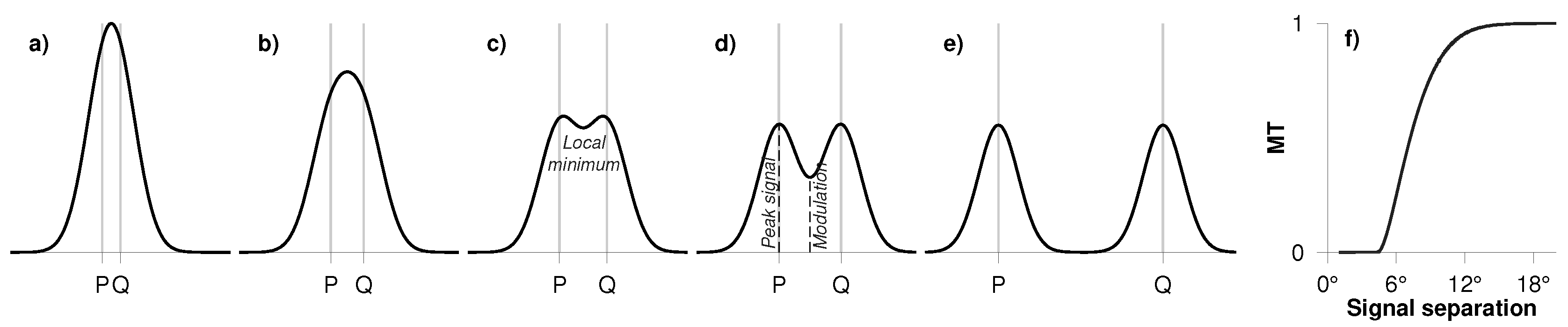
The problem of spatial resolution can be dealt with by treating the band-limit of the spherical harmonic spectrum as a spectral filter, and then by ascertaining the ideal spatial resolution of the filter [17]. Ideal spatial resolution of a filter is defined as the minimum distance required between two signals of equal magnitude, such that they are still seen as two different signals after filtering. The spatial resolution is closely tied to the contrast of the field, i.e., the prominence of the signals after filtering (cf. Figure 1), and, therefore, resolution is not just a number, but it is devised as a function of contrast (modulation) called the modulation transfer function (mtf) [17]. The mtf is a function of modulation transfer and separation between two signals of interest (cf. Figure 1):
The mtf helps us identify the minimum spherical distance (ideal resolution) between two Dirac pulses above which they are resolved as two distinct signals. Furthermore, from the slope of the mtf, the level of contrast that will be retained after filtering can also be ascertained—the steeper the slope, the more the contrast. Essentially, the ideal spatial resolution tells us that below this value any two signals of interest are indistinguishable. The MATLAB scripts (Mathworks, Natick, MA, USA) to compute mtf can be downloaded from http://gracebundle.tuxfamily.org.
The band-limited field in Equation (3) can be rewritten as a box-car filtered field as follows (see Appendix A for details):
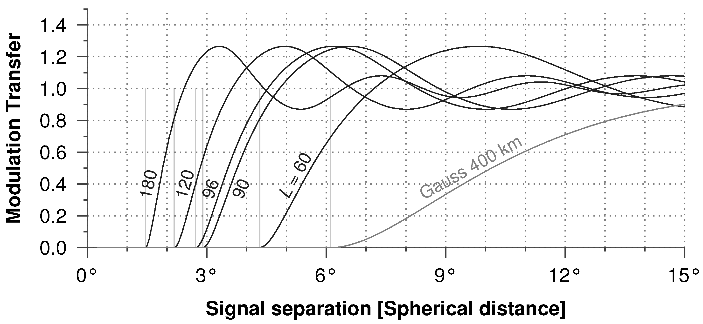
The degree-dependent spectrum when propagated to the spatial domain becomes the well-known Shannon kernel [39]. The mtf of the Shannon kernel for the typical grace bandwidths provides their ideal spatial resolution (cf. Figure 2), and, obviously, those numbers are higher than the half-wavelengths (sampling distance) that are usually used to designate their resolution (cf. Table 1). Since the Shannon kernel is a homogeneous and isotropic kernel (see Appendix A for definitions of homogeneous and isotropic), its ideal spatial resolution is also homogeneous and isotropic throughout the sphere [14]. Thus, with the ideal spatial resolution values, we are able to define the nominal size of features that can be clearly distinguished without ambiguity, and that they are valid throughout the sphere.
Due to their high noise levels, the grace monthly solutions are filtered prior to their use. Filtering suppresses noise, but, at the same time, has a damaging effect on the signal—it attenuates the signal, introduces leakage and changes the resolution. A Gaussian filter of half-width radius 400 km (3.6) has an ideal resolution of 680 km (6.1), which is far higher than the innate resolution of nearly all the typical band-limited grace fields (cf. Table 1). Due to signal attenuation, filtering also reduces signal contrast, which can be seen from the unfavourably gentle slope of the Gaussian mtf curve (cf. Figure 2).
2.3. Catchment Averages, Post-Filtering Corrections and Resolution
Thus far, the spatial resolution has been treated as a spherical distance, but it has to be translated into an areal quantity. As resolution of a band-limited field is isotropic, the area of the smallest resolvable feature will be a spherical cap with the diameter of the ideal spatial resolution. The spherical cap areas for typical grace bandwidths are given in Table 1.
The gridded grace products can be synthesized at a grid spacing smaller than the ideal spatial resolution. Therefore, it is logical to study the hydrological signal not at point scale, but rather at catchment scale [5,7,21]. It is common practice to compute a catchment average from the filtered field , which is written as
Since area aggregation is an operation performed over the spatial coordinates, the spherical harmonic spectrum is not tampered with. Therefore, it can be said with confidence that the minimum resolvable area does not change with the area aggregation operation.
The catchment average is computed for every epoch to obtain a time-series demonstrating the hydrological behaviour of the catchment. Since filtering damages the signal, the catchment scale products from filtered grace fields are corrected [5,8,19,20,21,24,25]. Filtering can be written as a convolution integral [11,14,21,40], and, loosely speaking, the repair scheme imitates a deconvolution process. Therefore, if the repair method does a good job, the resolution must improve. However, it is not a perfect process and that means we will not reach the ideal spatial resolution of the bandwidth, but it will definitely be better than that of the filtered field.
2.4. Some Exceptions
As mentioned earlier, satellite gravimetry does not image the field like optical/microwave remote sensing satellites, but provides it via geophysical inversion. Therefore, the values of spatial resolution are intricately tied to the inversion scheme. In the context of band-limited spherical harmonic representation of the grace observations, some key aspects have to be kept in mind while using or interpreting the values in Table 1 for catchment aggregated values. Small catchments
- 1.
- that have a strong seasonal variation in their water storage [7], or
- 2.
- that are similar in magnitude and temporal phase as their neighboring catchments, i.e., without spatial contrast [23] (it should not be confused with the signal contrast/modulation mentioned earlier), or
- 3.
- that are isolated or dominant in terms of their signal strength, for example huge reservoir volume changes [41]
can still be seen despite the resolution limitations of the given bandwidth.
For example, a small but strong signal source will be detected by the grace satellites, but, due to the band-limited nature of the spherical harmonic representation, the signal is spread over the area equivalent to the corresponding ideal resolution. The area aggregated value over such a catchment will contain a fair part of the signal from the catchment, and, depending on the above-mentioned conditions, it might as well be mixed with other sources in the vicinity. Therefore, such signal sources—catchments—can be studied with grace, but a priori information and signal segregation methods are needed to extract their full signal strength. This might be the reason that, for some very small catchments, Lorenz et al. [7] observe good correlation between the grace data and the mass change rate from the water balance equation, but with strong bias and significant differences in the amplitude.
3. Data and Method
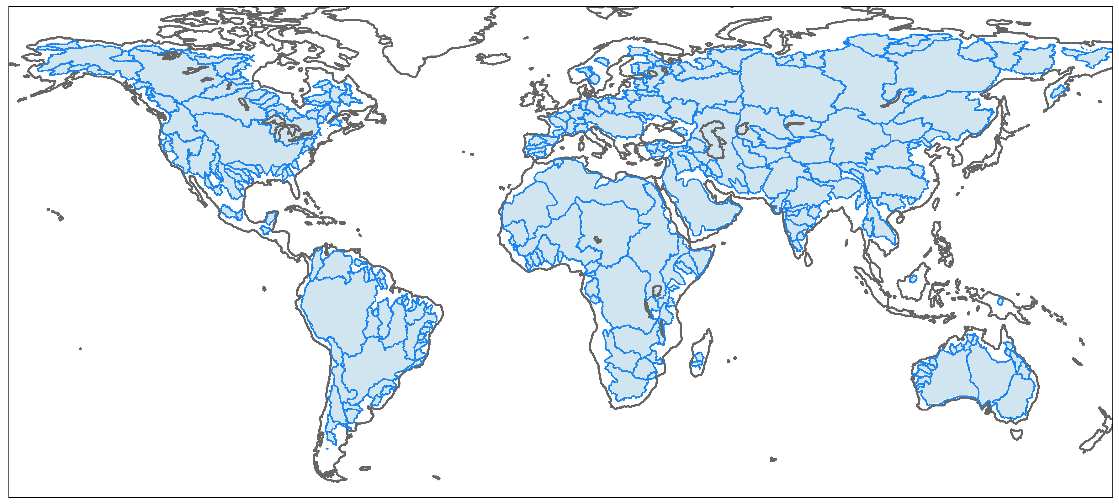
In order to use the relation between the accuracy and catchment size for identifying the spatial resolution of grace products in a comprehensive manner, we analyze more than 250 catchments shown in Figure 3. The largest catchment is the Amazon in South America with an area of ≈4,672,876 km and the smallest is Cavally catchment in West Africa with an area of ≈30,744 km. The study is carried out in a closed-loop simulation environment used by Vishwakarma et al. [21] and Vishwakarma et al. [25]. It consists of total water storage anomaly from the Global Land Data Assimilation System (gldas) Noah Land Surface Model as the background truth [42]. These global hydrological fields are contaminated with noise extracted from gfz grace fields [3]. In order to extract noise, we first filter the gfz grace fields with a destriping and a Gaussian filter [10], then we subtract the filtered fields from the corresponding noisy grace fields to derive a realistic grace-type noise. The grace-type noise is then added to the gldas model fields for 72 months to obtain grace-type noisy fields with known truth. Further details about the simulated field can be found in Vishwakarma et al. [21]. We can process the grace-type fields to obtain time-series for a catchment and it can be validated against the time-series from gldas fields. In this setup, we can assess the magnitude of error accurately because we have control over each component.
We filter the simulated grace-type noisy fields with a Gaussian filter and then compute catchment averages for 255 catchments to obtain the respective time-series. Let us denote the corrected time-series by . The true catchment average from the band-limited field is not known, but the regional average from the filtered field is known. One may approach true catchment average, which is approximately equal to the catchment average from the band-limited field, from catchment average of the filtered field with the help of correction methods. Out of many available methods, we choose four methods: the Multiplicative method by Longuevergne et al. [19], the scaling method by Landerer et al. [24], the additive method by Klees et al. [20], and the data-driven method by Vishwakarma et al. [25]. The mathematical relation that helps you correct for the signal damage due to filtering is given below:
| Multiplicative: | [19] | |
| Additive: | [20] | |
| Scaling: | [24] | |
| Data-driven: | [25]. |
The multiplicative method approaches corrected time-series by first removing leakage from catchment aggregate of filtered grace field , and then amplifying it by a scale factor s. Leakage is obtained from a hydrological model and the scale factor s is obtained from catchment mask and filtered catchment mask:
where is the catchment mask: 1 inside and 0 outside, is the filtered catchment mask, is the domain of the surface of the Earth, and is the infinitesimal surface element .
The additive method approaches corrected time-series by subtracting leakage from the catchment aggregate of filtered grace field and adding bias , where both leakage and bias are obtained from a hydrological model. The scaling method approaches corrected time-series by multiplying grace products by a scale factor k that is obtained by estimating a multiplicative factor, between a hydrological model and its filtered version, via least squares estimation.
The data-driven method corrects time-series by removing leakage and deviation integral from the catchment average of filtered grace fields . To compute the leakage and the deviation integral, we do not rely on hydrological models, but use the grace fields only. Here, one may argue that the grace fields are noisy, thus the leakage and the deviation integral computed from noisy fields will not be accurate. This is the reason they are computed from filtered grace fields. Since we know that the filtered grace fields are not equal to the truth, the leakage and the deviation integral from these fields are also not accurate. However, Vishwakarma et al. [25] demonstrated that if we multiply the leakage and the deviation integral from filtered grace fields, by a scalar ratio between the leakage and the deviation integral from once filtered grace fields and twice filtered grace fields, we can approach near-truth leakage and deviation integral. Although this approximation works for most of the catchments, it has limitations over arid regions and the estimated leakage and deviation integral for these regions is less accurate. Nevertheless, the accuracy of data-driven methods is still either at par or better than what we can achieve from other methods [25]. Please refer to Vishwakarma et al. [25] and Vishwakarma et al. [21] for more information. Since the multiplicative, the additive, and the scaling approach use a hydrological model to estimate corrected time-series, we call them model-dependent approaches, while the data-driven approach uses grace fields only and do not depend on models, we can also call it model-independent.
Global hydrological models have huge uncertainties that vary in space and in time, which is responsible for their differences with grace fields [43]. Using these models for correcting grace products brings their uncertainty to the final grace product. In order to imitate the impact of using a model for correcting grace, we prefer not to use the gldas model that is also the background truth; instead, we use the WaterGAP hydrological model (wghm model [44]) to compute model-dependent correction terms employed by model-dependent methods. The data-driven method computes its correction terms, leakage and the deviation integral , from once filtered and twice filtered grace-type noisy fields. The MATLAB scripts for the data-driven method can be downloaded from https://www.researchgate.net/publication/324804360MatlabscriptsDatadriven or from Institute of Geodesy, Stuttgart web page http://www.gis.uni-stuttgart.de/research/projects/DataDrivenCorrection/.
The corrected time-series from the above-mentioned four methods is compared to the truth obtained from gldas model fields for 255 catchments. The following statistical measures are computed to characterize the behavior of difference (error) between the corrected time-series and the true time-series with respect to the catchment size:
- Root Mean Square of Error (RMSE):
- Cyclostationary Nash–Sutcliffe Efficiency () [45,46]:where represents the true value obtained from gldas fields, is the mean annual behaviour (mean monthly values) and m is the number of epochs. RMSE can attain any positive value, a RMSE close to zero represents excellent agreement between and . can attain any value between and 1. A positive value indicates that the difference between the true signal () and the corrected time-series () is well below the non-seasonal variations in the time-series. Typically, hydrological signals have a clear seasonal signal, i.e., change in the amplitude and/or sign of the signal from the summer months to the winter months. However, every summer/winter is not the same and there is a random variation in the amplitude of the signal from year-to-year, which is the non-seasonal variation (the natural variability of the signal). When the error in corrected time-series is smaller than this natural variability, then we can conclude that the signal is very well restored. If we were to use the as proposed by Nash and Sutcliffe [47], without accounting for the cyclostationary seasonal signal, the differences will be compared to the amplitudes of the annual signal. This will not provide a proper indicator for the efficacy of the repairing schemes.
4. Results and Discussion
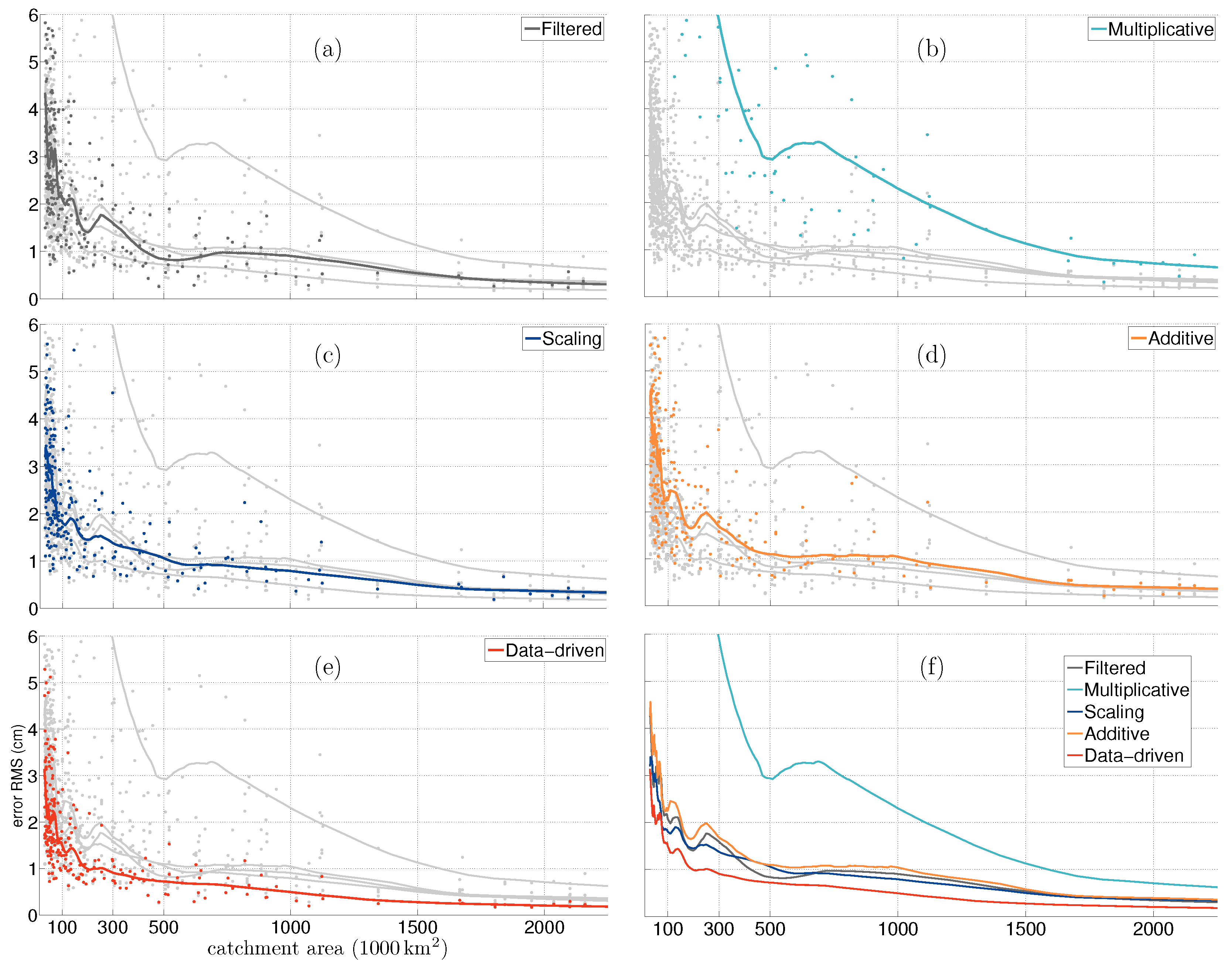
In Figure 4 and Figure 5, we have plotted the RMSE and the for four corrected time-series and time-series from filtered fields over 255 catchments. The catchments are sorted by their area. Since the scatter of these statistical measures is wide, we fit a smooth line, obtained by using locally weighted scatter-plot smoothing (LOESS), to identify the general pattern. LOESS is a non-parametric method that uses iterative locally weighted regression to fit a second degree polynomial through points in a scatter plot [48]. Since the number of large catchments is smaller than the number of small catchments, the data points on the x-axis, i.e., catchment area, suffer from unequal intervals. Therefore, we have defined bins to counter this irregular data distribution. The first bin is for catchments from 30,000 km to 100,000 km with sample points every 1000 km, the next bin is for catchments from 100,000 km to 1,000,000 km with sample point every 10,000 km, and the last bin is for catchment from 1,000,000 km to 4,000,000 km with sample points every 100,000 km. A window size of 51 is used for smoothing. We have chosen these parameters to obtain a smooth fit that would represent the general behaviour of the scatter.
We can observe that the error, in general, increases as the area of the catchment decreases, irrespective of the correction method used. However, the rate at which the error increases varies from one method to the other. The multiplicative approach, due to a larger scale factor for smaller catchment, experiences a steep decay in performance. The additive approach, the scaling approach and the time-series from filtered fields are competitive. However, the data-driven method is able to provide better mass change estimates at all catchment scales.
Although, in general, the disagreement between the corrected and the true time-series increases as the catchment size decreases, several small catchments exhibit less error in comparison to a few relatively large catchments. The magnitude of error corresponding to a catchment is pertinent to this simulation setup, and it will change a little bit if we change the background models and simulation setup. Nevertheless, the general pattern that error increases as catchment size decreases will hold.
Ideally, with no noise and no approximations, we expect to recover the full band-limited signal after applying the data-driven method (see Figure 3, Vishwakarma et al. [25]). However, in reality, we lose some accuracy and the error is not zero even for the largest catchment Amazon. The error in the corrected time-series, for catchments smaller than the resolution of the filtered field and larger than the ideal resolution of band-limited grace data, should be close to the error in time-series from filtered fields for larger catchments. We can use the trade-off between accuracy and the catchment size to discuss the potential grace resolution: those catchments with an error less than a defined threshold can be categorized as resolvable.
Let us say we can accept the grace products for all the catchments with an RMSE better than a certain value, say or . We leave it to the user to define the maximum tolerable error for their application and then decide whether the catchment or region of interest is suitable for analysis with grace products corrected with a certain repair scheme. For example, if we choose as the error limit, then filtered products can be used to monitor catchments larger than ≈750,000 km, a multiplicative approach can be used for catchments larger than ≈1,563,000 km, an additive approach for catchments larger than ≈1,103,000 km, a scaling approach for catchments larger than ≈563,000 km and the data-driven method for catchments larger than ≈250,000 km. If the tolerable error is , then the limit is ≈152,000 km for filtered and additive, ≈810,000 km for multiplicative and ≈63,000 km for both scaling and the data-driven method. In Table 2, we have summarized the resolvable catchment corresponding to an error level.
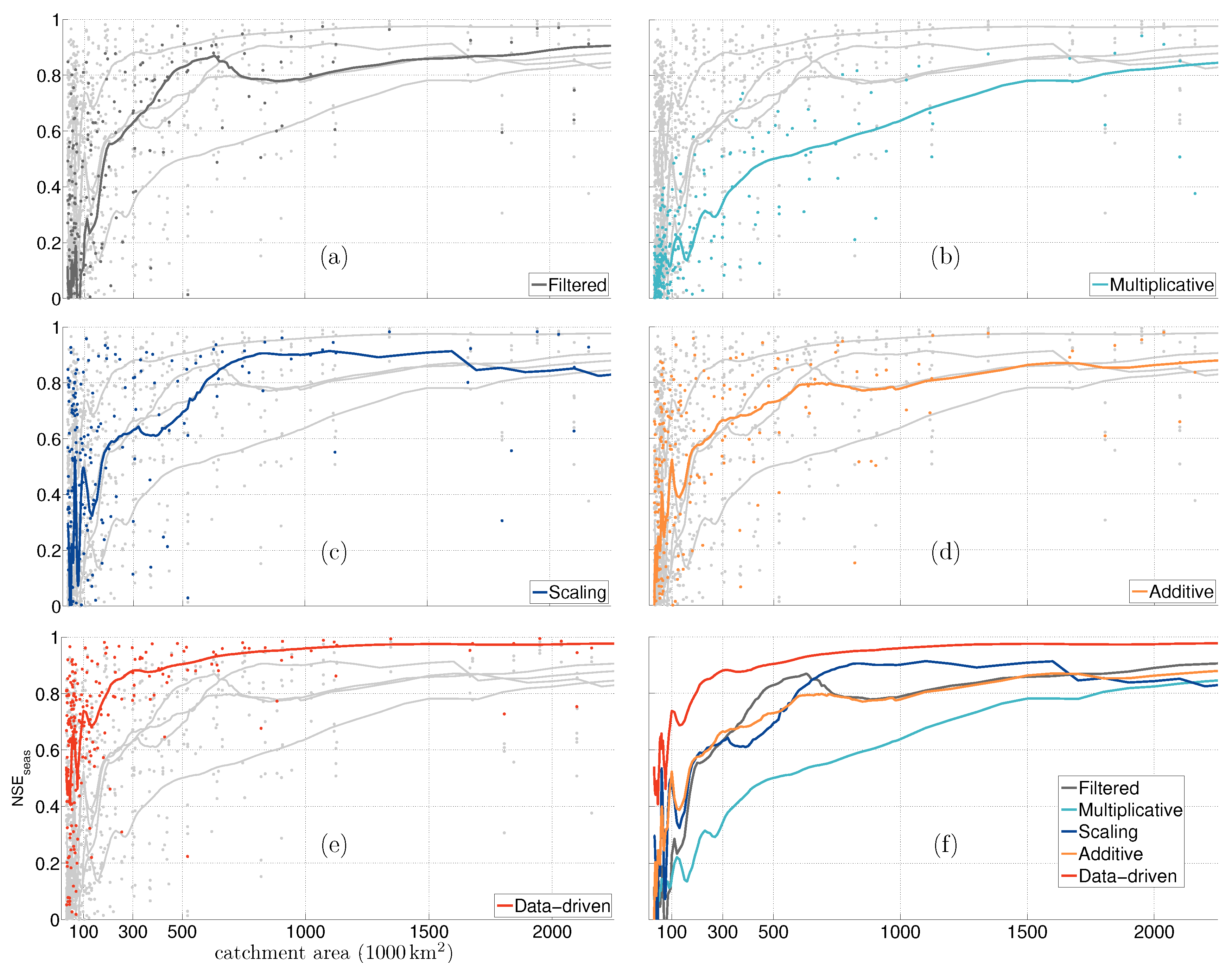
Since accounts for both the difference in the magnitude and the correlation between the corrected and the true time-series, it is a powerful indicator and popularly used in time-series analysis. One may choose an acceptable value for their application to determine the corresponding spatial resolution. For example, if we choose 0.8 as an acceptable limit, then filtered products can be used to monitor catchments larger than ≈1,100,000 km, a multiplicative approach can be used for catchments larger than ≈1,750,500 km, an additive approach for catchments larger than ≈1,100,500 km, a scaling approach for catchments larger than ≈600,000 km and the data-driven method for catchments larger than ≈200,000 km. In Table 3, we have provided the approximate spatial resolution corresponding to a value. It is to be noted that the LOESS fit for the multiplicative approach and for the additive approach never attain value of 0.9. Furthermore, the spatial resolution improves with increasing values, while the corresponding RMSE decreases.
These limits on the spatial resolution are obtained, from Figure 4 and Figure 5, by observing the point at which the fit crosses a RMSE value or a value for the first time. Thus, the values in Table 2 and Table 3 are only meaningful if the LOESS fit is smooth; as soon as the fit seems noisy, we should be careful in interpreting the resolvable catchment size. Therefore, in this analysis, we have ignored all the catchments for which the fit tends to be noisy—for example, the fit for the data-driven method becomes noisy for catchments below ≈600,000 km. We can find a lower resolvable catchment area for the data-driven method corresponding to an RMSE level of , but this part of the fit is noisy and we avoid any interpretation. Please note that, within these suggested spatial resolution limits, where one can choose from many methods, one method may perform better than the others as per the fit. Such a general rule can be used but with the understanding that individual catchments may deviate from the defined error behaviour. This is shown by the disagreement between the scatter and the fit.
5. Conclusions
The grace satellite mission has helped us observe continental scale hydrology. Moreover, with improved data processing skills, we have been able to use grace products for monitoring catchment scale hydrology. Although the spatial resolution of grace is accepted to be coarse, it was necessary to put a number to the spatial resolution of the band-limited grace fields and of the filtered grace fields. It was established by previous contributions that ideal spatial resolution can be used to define their spatial resolutions.
Notwithstanding this, there have been many attempts to identify the potential spatial resolution of the grace products in terms of catchment size, but every attempt concluded with a different number. The difference in the research findings can be attributed to usage of different processing methods and selective regional analysis. For example, one can choose a filter out of many available ones and then a corrective method for repairing the signal damage due to the filtering. Thus, the end product is influenced by combined effects of different processes and it is hard to quantify whether the final product is able to resolve a catchment efficiently. With developments in post-processing algorithms for grace data, it was necessary to understand the contemporary spatial resolving power of grace products. This study provides a comprehensive analysis of grace products corrected with different repairing schemes to demarcate the catchment size that can be effectively observed. We have carried out such an analysis for 255 catchments of small to very large size in a closed-loop simulation environment, in order to answer the question of what is the minimum size of catchment that can be observed with the help of improved grace products.
We found that in general the error increases as the catchment size decreases, but the error level varies from one repair method to the other. grace time-series corrected with multiplicative approach shows the highest amount of error and the grace time-series from the data-driven approach has the lowest amount of error. We discussed the effective resolution of corrected grace products with respect to an acceptable error threshold. We found that the data-driven method and scaling method were able to approach the ideal grace resolution with an acceptable error RMSE level of . The data-driven method has minimum divergence in terms of the spatial resolution with respect to the performance indicators (RMSE and ).
Therefore, based on our investigation and its findings, we recommend the following:
- 1.
- The spatial resolution of the band-limited grace spherical harmonics is not the half-wavelength at the equator, but the ideal spatial resolution. The spatial resolution of filtered grace data can also be described by the ideal spatial resolution.
- 2.
- The users have to be wary that the spatial resolution of the corrected dataset is dependent on the adopted method. Furthermore, the spatial resolution is associated with the error tolerance required by the application and it has to be defined by the user.
- 3.
- Given the fact that with enhanced processing techniques grace is able to see some catchments smaller than the spatial resolution and many catchments close to the band-limit resolution, it is worthwhile to provide spherical harmonics up to a maximum degree of 120 or higher.
The impending launch of the grace-Follow On mission, which is a near replica of the grace mission with only the Laser Ranging Instrument as the additional instrument, raises the question of the relevance of this study for grace-fo data. Recently, a simulation study by Flechtner et al. [49] indicated that the expected improvement from grace-fo is rather moderate, in which case we expect our quantitative results to hold even for grace-fo data. Having said that, the mathematical foundation and the understanding of the idea of spatial resolution developed in this study will always be relevant for data disseminated in terms of spherical harmonic coefficients.
Author Contributions
B.D.V. conceived the project. B.D.V. and B.D. designed the study. B.D.V. simulated the data and computed the results. B.D.V. and B.D. wrote the manuscript. All the authors discussed the results and commented critically on the manuscript.
Acknowledgments
In this work, we have made use of catchment boundaries from GRDC (http://www.bafg.de/GRDC/EN/02srvcs/22gslrs/221MRB/riverbasinsnode.html). We have also used the hydrological model gldas from ldas.gsfc.nasa.gov/gldas/, which used the Goddard Earth Sciences Data and Information Services Center. We are thankful to Döll et al. [44] for providing us with wghm hydrological model data. Balaji Devaraju would like to thank the DFG Sonderforschungsbereich (SFB) 1128 Relativistic Geodesy and Gravimetry with Quantum Sensors (geo-Q) for financial support.
Conflicts of Interest
The authors declare no conflict of interest.
Appendix A. Filtering on the Sphere
The dominance of noise in the grace monthly solutions is suppressed by applying low-pass filters. The central idea behind these filters is the weighted averaging using weighting windows defined on the sphere, and it is expressed in mathematical form as follows [8]:
where is the noisy field; is the filter kernel; and are the corresponding spectra of the field and the filter; are the normalized associated Legendre functions; and is the filtered field [8].
Figure A1.
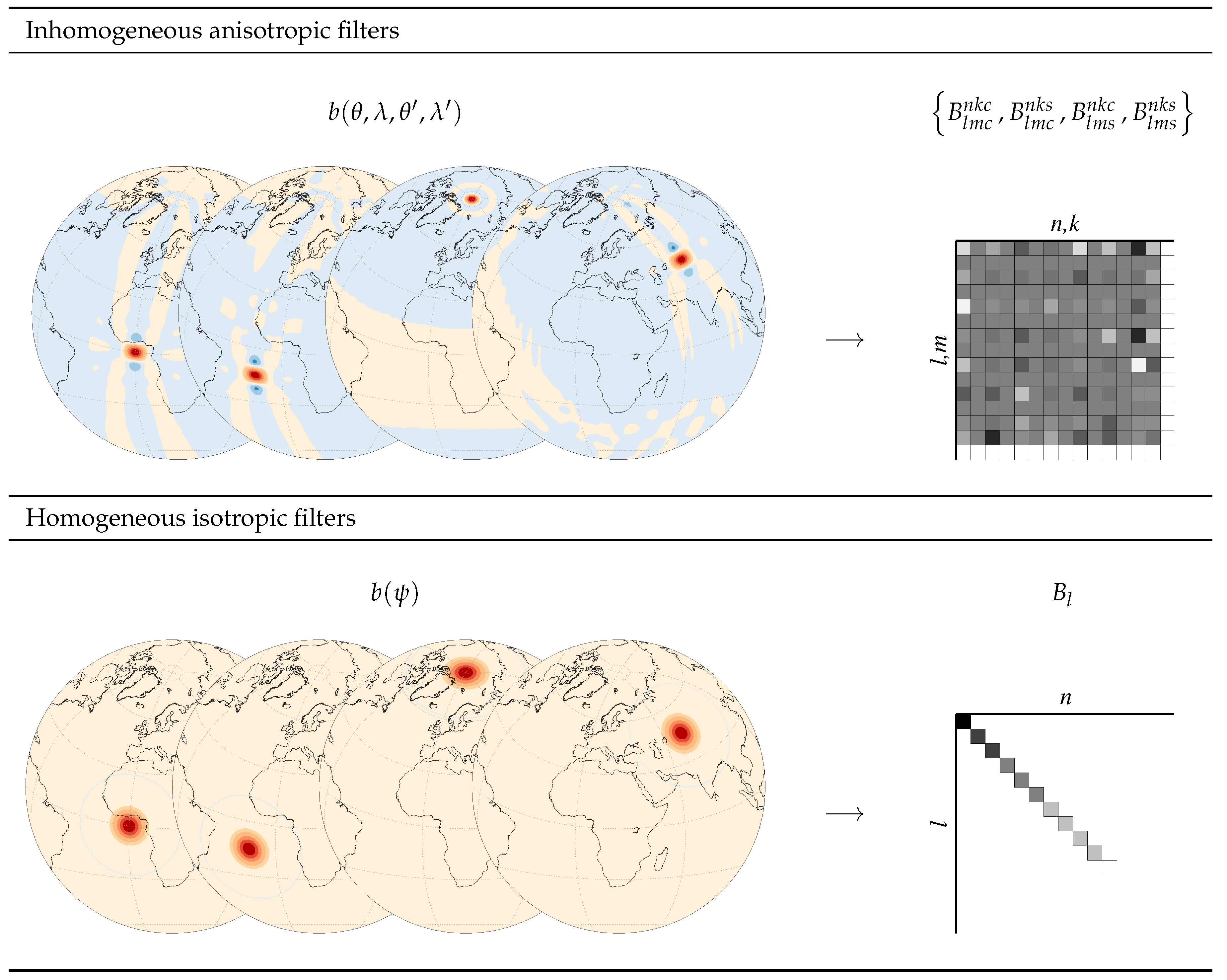
The concepts of homogeneity/inhomogeneity and isotropy/anisotropy of the filter weights is illustrated here with the most general form of the filter function (inhomogeneous and ansiotropic) in the top row and the simplest form of the filter function (homogeneous and isotropic) in the bottom row.
Figure A1.
The concepts of homogeneity/inhomogeneity and isotropy/anisotropy of the filter weights is illustrated here with the most general form of the filter function (inhomogeneous and ansiotropic) in the top row and the simplest form of the filter function (homogeneous and isotropic) in the bottom row.

The filter function is a two-point function that describes the relative weight between the calculation point and the data point. The calculation point is where we want the filtered which is computed by averaging all the data points by applying the weights on the data points. The filter function can also be represented in polar co-ordinate system , where the pole is the calculation point, and the data points are related to the calculation point by the angular distance and A the azimuth.
The filter function described in Equation (A3) is the most general form of the filter, where the weights of the data points depend on the location of the calculation point, the angular distance as well as the azimuth. However, in the case of the grace data processing, the most commonly used Gausssian filter is a special type of filter that is classified as homogeneous isotropic filter. The weights of such special filters depend only on the spherical distance between the calculation and data points. They are independent of the location of the calculation point (homogeneous) and also of the azimuth (isotropic) (cf. Figure A1).
The spectrum of the homogeneous isotropic filters, due to their dependence only on the spherical distance, becomes dependent only on the spherical harmonic degree [14,50]:
where are the unnormalized Legendre polynomials of spherical harmonic degree l and are the coefficients of the homogeneous isotropic filter. Notice that there is only one index as opposed to four in Equation (A3). A field filtered with a homogeneous isotropic filter will have the following spectrum:
where we see that the unfiltered spectrum is scaled by the filter spectrum for every spherical harmonic degree, as opposed to the general form of the filter (cf. (A2)). Equation (A5) is the same as Equation (7), and, therefore, all the band-limited fields have the properties of a field filtered with a homogeneous and isotropic filter. Since the fields filtered with a homogeneous isotropic filter have a homogeneous and isotropic spatial resolution, the spatial resolution of the band-limited fields is also homogeneous and isotropic.
References
- Famiglietti, J.S. The global groundwater crisis. Nat. Clim. Chang. 2014, 4, 945–948. [Google Scholar] [CrossRef]
- Sneeuw, N.; Lorenz, C.; Devaraju, B.; Tourian, M.J.; Riegger, J.; Kunstmann, H.; Bárdossy, A. Estimating Runoff Using Hydro-Geodetic Approaches. Surv. Geophys. 2014, 35, 1333–1359. [Google Scholar] [CrossRef]
- Dahle, C.; Flechtner, F.; Gruber, C.; König, D.; König, R.; Michalak, G.; Neumayer, K.H. GFZ GRACE Level-2 Processing Standards Document for Level-2 Product Release 05; Scientific Technical Report-Data 12/02; GFZ: Potsdam, Germany, 2012. [Google Scholar]
- Mayer-Gürr, T.; Behzadpour, S.; Ellmer, M.; Kvas, A.; Klinger, B.; Zehentner, N. ITSG-Grace2016—Monthly and Daily Gravity Field Solutions from GRACE. Website, GFZ Data Services, 2016. Available online: https://www.tugraz.at/institute/ifg/downloads/gravity-field-models/itsg-grace2016/ (accessed on 30 April 2017).
- Swenson, S. Methods for inferring regional surface-mass anomalies from Gravity Recovery and Climate Experiment (GRACE) measurements of time-variable gravity. J. Geophys. Res. 2002, 107, 2193. [Google Scholar] [CrossRef]
- Wahr, J.; Swenson, S.; Velicogna, I. Some Hydrological and Cryospheric Applications of GRACE. In Proceedings of the GRACE Science Team Meeting and DFG SPP1257 Symposium, Potsdam, Germany, 15–17 October 2007. [Google Scholar]
- Lorenz, C.; Devaraju, B.; Tourian, M.J.; Sneeuw, N.; Riegger, J.; Kunstmann, H. Large-scale runoff from landmasses: A global assessment of the closure of the hydrological and atmospheric water balances. J. Hydrometeorol. 2014, 15, 2111–2139. [Google Scholar] [CrossRef]
- Wahr, J.; Molenaar, M.; Bryan, F. Time variability of the Earth’s gravity field: Hydrological and oceanic effects and their possible detection using GRACE. J. Geophys. Res. 1998, 103, 30205. [Google Scholar] [CrossRef]
- Han, S.C.; Shum, C.K.; Jekeli, C.; Kuo, C.Y.; Wilson, C.; Seo, K.W. Non-isotropic filtering of GRACE temporal gravity for geophysical signal enhancement. Geophys. J. Int. 2005, 163, 18–25. [Google Scholar] [CrossRef]
- Swenson, S.; Wahr, J. Post-processing removal of correlated errors in GRACE data. Geophys. Res. Lett. 2006, 33, L08402. [Google Scholar] [CrossRef]
- Kusche, J. Approximate decorrelation and non-isotropic smoothing of time-variable GRACE-type gravity field models. J. Geod. 2007, 81, 733–749. [Google Scholar] [CrossRef]
- Klees, R.; Revtova, E.A.; Gunter, B.C.; Ditmar, P.; Oudman, E.; Winsemius, H.C.; Savenije, H.H.G. The design of an optimal filter for monthly GRACE gravity models. Geophys. J. Int. 2008, 175, 417–432. [Google Scholar] [CrossRef]
- Zhang, Z.Z.; Chao, B.F.; Lu, Y.; Hsu, H.T. An effective filtering for GRACE time-variable gravity: Fan filter. Geophys. Res. Lett. 2009, 36, L17311. [Google Scholar] [CrossRef]
- Devaraju, B. Understanding Filtering on the Sphere—Experiences from Filtering GRACE Data. Ph.D. Thesis, Universität Stuttgart, Stuttgart, Germany, 2015. [Google Scholar]
- Werth, S.; Güntner, A.; Schmidt, R.; Kusche, J. Evaluation of GRACE filter tools from a hydrological perspective. Geophys. J. Int. 2009, 179, 1499–1515. [Google Scholar] [CrossRef]
- Klees, R.; Liu, X.; Wittwer, T.; Gunter, B.C.; Revtova, E.A.; Tenzer, R.; Ditmar, P.; Winsemius, H.C.; Savenije, H.H.G. A Comparison of Global and Regional GRACE Models for Land Hydrology. Surv. Geophys. 2008, 29, 335–359. [Google Scholar] [CrossRef]
- Devaraju, B.; Sneeuw, N. On the Spatial Resolution of Homogeneous Isotropic Filters on the Sphere. In Proceedings of the VIII Hotine-Marussi Symposium on Mathematical Geodesy, Rome, Italy, 17–21 June 2013; Sneeuw, N., Novák, P., Crespi, M., Sansò, F., Eds.; Springer: Cham, Switzerland, 2016; pp. 67–73. [Google Scholar]
- King, M.; Moore, P.; Clarke, P.; Lavallée, D. Choice of optimal averaging radii for temporal GRACE gravity solutions, a comparison with GPS and satellite altimetry. Geophys. J. Int. 2006, 166, 1–11. [Google Scholar] [CrossRef]
- Longuevergne, L.; Scanlon, B.R.; Wilson, C.R. GRACE Hydrological estimates for small basins: Evaluating processing approaches on the High Plains Aquifer, USA. Water Resour. Res. 2010, 46, W11517. [Google Scholar] [CrossRef]
- Klees, R.; Zapreeva, E.A.; Winsemius, H.C.; Savenije, H.H.G. The bias in GRACE estimates of continental water storage variations. Hydrol. Earth Syst. Sci. 2007, 11, 1227–1241. [Google Scholar] [CrossRef]
- Vishwakarma, B.D.; Devaraju, B.; Sneeuw, N. Minimizing the effects of filtering on catchment scale GRACE solutions. Water Resour. Res. 2016, 52, 5868–5890. [Google Scholar] [CrossRef]
- Long, D.; Longuevergne, L.; Scanlon, B.R. Global analysis of approaches for deriving total water storage changes from GRACE satellites. Water Resour. Res. 2015, 51, 2574–2594. [Google Scholar] [CrossRef] [Green Version]
- Vishwakarma, B.D. Understanding and Repairing the Signal Damage Due to Filtering of Mass Change Estimates from the GRACE Satellite Mission. Ph.D. Thesis, University of Stuttgart, Stuttgart, Germany, 2017. [Google Scholar]
- Landerer, F.W.; Swenson, S.C. Accuracy of scaled GRACE terrestrial water storage estimates. Water Resour. Res. 2012, 48, W04531. [Google Scholar] [CrossRef]
- Vishwakarma, B.D.; Horwath, M.; Devaraju, B.; Groh, A.; Sneeuw, N. A Data-Driven Approach for Repairing the Hydrological Catchment Signal Damage Due to Filtering of GRACE Products. Water Resour. Res. 2017, 53, 9824–9844. [Google Scholar] [CrossRef]
- Horwath, M.; Dietrich, R. Signal and error in mass change inferences from GRACE: The case of Antarctica. Geophys. J. Int. 2009, 177, 849–864. [Google Scholar] [CrossRef]
- Baur, O.; Kuhn, M.; Featherstone, W.E. GRACE-derived ice-mass variations over Greenland by accounting for leakage effects. J. Geophys. Res. Solid Earth 2009, 114, B06407. [Google Scholar] [CrossRef]
- King, A.M.; Bingham, J.R.; Moore, P.; Whitehouse, L.P.; Bentley, J.M.; Milne, A.G. Lower satellite-gravimetry estimates of Antarctic sea-level contribution. Nature 2012, 491, 586–589. [Google Scholar] [CrossRef] [PubMed]
- Chen, J.L.; Wilson, C.R.; Li, J.; Zhang, Z. Reducing leakage error in GRACE-observed long-term ice mass change: A case study in West Antarctica. J. Geod. 2015, 89, 925–940. [Google Scholar] [CrossRef]
- Schmidt, R.; Flechtner, F.; Meyer, U.; Neumayer, K.H.; Dahle, C.; König, R.; Kusche, J. Hydrological Signals Observed by the GRACE Satellites. Surv. Geophys. 2008, 29, 319–334. [Google Scholar] [CrossRef]
- Rowlands, D.D.; Luthcke, S.B.; Klosko, S.M.; Lemoine, F.G.R.; Chinn, D.S.; McCarthy, J.J.; Cox, C.M.; Anderson, O.B. Resolving mass flux at high spatial and temporal resolution using GRACE intersatellite measurements. Geophys. Res. Lett. 2005, 32, L04310. [Google Scholar] [CrossRef]
- Tourian, M.; Elmi, O.; Chen, Q.; Devaraju, B.; Roohi, S.; Sneeuw, N. A spaceborne multisensor approach to monitor the desiccation of Lake Urmia in Iran. Remote Sens. Environ. 2015, 156, 349–360. [Google Scholar] [CrossRef]
- Khaki, M.; Forootan, E.; Kuhn, M.; Awange, J.; Longuevergne, L.; Wada, Y. Efficient basin scale filtering of GRACE satellite products. Remote Sens. Environ. 2018, 204, 76–93. [Google Scholar] [CrossRef]
- Heiskanen, W.A.; Moritz, H. Physical Geodesy; W. H. Freeman and Company: San Francisco, CA, USA, 1967. [Google Scholar]
- Weigelt, M.; Sneeuw, N.; Schrama, E.J.O.; Visser, P.N.A.M. An improved sampling rule for mapping geopotential functions of a planet from a near polar orbit. J. Geod. 2013, 87, 127–142. [Google Scholar] [CrossRef]
- Colombo, O.L. Numerical Methods for Harmonic Analysis on the Sphere; Technical Report 310; Department of Geodetic Science, The Ohio State University: Columbus, OH, USA, 1981. [Google Scholar]
- Sneeuw, N. Global spherical harmonic analysis by least squares and numerical quadrature methods in historical perspective. Geophys. J. Int. 1994, 118, 707–716. [Google Scholar] [CrossRef]
- McEwen, J.D.; Wiaux, Y. A Novel Sampling Theorem on the Sphere. IEEE Trans. Signal Process. 2011, 59, 5876–5887. [Google Scholar] [CrossRef]
- Freeden, W.; Schreiner, M. Spherical functions of mathematical geosciences. In Advances in Geophysical and Environmental Mechanics and Mathematics; Springer: Berlin, Germany, 2009; p. 602. [Google Scholar]
- Jekeli, C. Alternative Methods to Smooth the Earth’s Gravity Field; Technical Report 327; Department of Geodetic Science and Surveying, The Ohio State University: Columbus, OH, USA, 1981. [Google Scholar]
- Yi, S.; Song, C.; Wang, Q.; Wang, L.; Heki, K.; Sun, W. The potential of GRACE gravimetry to detect the heavy rainfall-induced impoundment of a small reservoir in the upper Yellow River. Water Resour. Res. 2017, 53, 6562–6578. [Google Scholar] [CrossRef]
- Rodell, M.; Houser, P.R.; Jambor, U.; Gottschalck, J.; Mitchell, K.; Meng, C.J.; Arsenault, P.R.; Cosgrove, B.; Radakovich, J.; Bosilovich, M.; et al. The Global Land Data Assimilation System. Bull. Am. Meteorol. Soc. 2004, 85, 381–394. [Google Scholar] [CrossRef]
- Werth, S. Calibration of the Global Hydrological Model WGHM with Water Mass Variations from GRACE Gravity Data. Ph.D. Thesis, Universität Potsdam, Potsdam, Germany, 2010. [Google Scholar]
- Döll, P.; Müller Schmied, H.; Schuh, C.; Portmann, F.T.; Eicker, A. Global-scale assessment of groundwater depletion and related groundwater abstractions: Combining hydrological modeling with information from well observations and GRACE satellites. Water Resour. Res. 2014, 50, 5698–5720. [Google Scholar] [CrossRef]
- Thor, R. Least-Squares Prediction of Runoff. Bachelor’s Thesis, University of Stuttgart, Stuttgart, Germany, 2013. [Google Scholar]
- Lorenz, C.; Tourian, M.J.; Devaraju, B.; Sneeuw, N.; Kunstmann, H. Basin-scale runoff prediction: An Ensemble Kalman Filter framework based on global hydrometeorological data sets. Water Resour. Res. 2015, 51, 8450–8475. [Google Scholar] [CrossRef]
- Nash, J.E.; Sutcliffe, J.V. River flow forecasting through conceptual models part I—A discussion of principles. J. Hydrol. 1970, 10, 282–290. [Google Scholar] [CrossRef]
- Cleveland, R.; Cleveland, W.; McRae, J.; Terpenning, I. STL: A Seasonal-Trend Decomposition Procedure Based on Loess (with Discussion). J. Off. Stat. 1990, 6, 3–73. [Google Scholar]
- Flechtner, F.; Neumayer, K.H.; Dahle, C.; Dobslaw, H.; Fagiolini, E.; Raimondo, J.C.; Güntner, A. What Can be Expected from the GRACE-FO Laser Ranging Interferometer for Earth Science Applications? Surv. Geophys. 2016, 37, 453–470. [Google Scholar] [CrossRef]
- Rummel, R.; Schwarz, K.P. On the nonhomogeneity of the global covariance function. Bull. Geod. 1977, 51, 93–103. [Google Scholar] [CrossRef]
Figure 1.
Illustration of the ideal spatial resolution computation for filter windows. Two Dirac pulses (gray lines in (a–e)) are set up at points P and Q and the field is filtered (black lines in (a–e)). For a given filter, they are resolved as two different signals at a certain separation (c)—the ideal spatial resolution. However, the signals are more prominent after filtering (contrast), if the distance between the signals is larger (d,e). The contrast is quantified via the modulation transfer function (mtf), which is a function of the modulation transfer (cf. (6)) and signal separation (f).

Figure 2.
The modulation transfer functions of the Shannon kernels corresponding to the most common bandwidths of the grace spherical harmonic spectra. A modulation transfer of 0 means that the two Dirac pulses separated by those distances will not be resolved, and a modulation transfer of 1 means that the signals are completely resolved and their contrast completely retained. The light-gray lines indicate the ideal resolution of the corresponding kernels.

Figure 3.
Distribution of 255 catchments used in this study. The catchments are filled in light blue with the boundary in blue. The catchment boundaries were downloaded from Global Runoff Data Centre (GRDC) website.
Figure 3.
Distribution of 255 catchments used in this study. The catchments are filled in light blue with the boundary in blue. The catchment boundaries were downloaded from Global Runoff Data Centre (GRDC) website.

Figure 4.
RMSE and corresponding fit with respect to the catchment area for different correction methods. Subplots (a) to (e) show RMSE and corresponding fit for one method in colour and others in gray. Subplot (f) compares the fit for different methods.
Figure 4.
RMSE and corresponding fit with respect to the catchment area for different correction methods. Subplots (a) to (e) show RMSE and corresponding fit for one method in colour and others in gray. Subplot (f) compares the fit for different methods.

Figure 5.
and corresponding fit with respect to the catchment area for different correction methods. Subplots (a) to (e) show and corresponding fit for one method in colour and others in gray. Subplot (f) compares the fit for different methods.
Figure 5.
and corresponding fit with respect to the catchment area for different correction methods. Subplots (a) to (e) show and corresponding fit for one method in colour and others in gray. Subplot (f) compares the fit for different methods.


Table 1.
Comparison of the half-wavelength and ideal spatial resolution values for typical grace bandwidths. Also shown are the typical area associated with them. The area of an equi-angular grid cell centered on the equator () is associated with the half-wavelength, and the spherical area () is associated with the ideal spatial resolution. N/A stands for not applicable.
| L | Half-Wavelength | Ideal Spatial Resolution | |||||
|---|---|---|---|---|---|---|---|
| [1000 km] | [km] | [1000 km] | [km] | ||||
| 60 | 3 | 111.5 | 334 | 182.4 | 427 | ||
| 90 | 2 | 49.6 | 223 | 81.9 | 286 | ||
| 96 | 1 | 43.6 | 209 | 72.0 | 268 | ||
| 120 | 1 | 27.9 | 167 | 46.2 | 215 | ||
| 180 | 1 | 12.4 | 111 | 20.7 | 144 | ||
| Gauss 400 km | n/a | n/a | n/a | 363.2 | 603 | ||
Table 2.
The approximate resolvable catchment size (in 1000 km) for a repair method performing better than a given RMSE. The values given here are obtained from the fit, and one should be more careful while carrying out studies for catchments close to the limit as the scatter is wide. Our suggestion is to avoid any interpretation after the fit tends to become noisy. When the fit for a method becomes noisy, we represent it by writing N/A.
| RMSE () | Filtered | Multiplicative | Additive | Scaling | Data-Driven |
|---|---|---|---|---|---|
| 1 | 750 | 1563 | 1103 | 563 | 250 |
| 1.5 | 337 | 1323 | 360 | 260 | 152 |
| 2 | 152 | 1103 | 152 | 90 | 63 |
| 2.5 | 90 | 951 | 1223 | 76 | N/A |
| 3 | N/A | 810 | N/A | N/A | N/A |
Table 3.
The approximate resolvable catchment size (in 1000 km) for a repair method performing better than a given . The values given here are obtained from the fit, and one should be more careful while carrying out studies for catchments close to the limit as the scatter is wide. Our suggestion is to avoid any interpretation after the fit tends to become noisy. When the fit for a method becomes noisy, we represent it by writing N/A.
| Filtered | Multiplicative | Additive | Scaling | Data-Driven | |
|---|---|---|---|---|---|
| 0.9 | 2000 | – | – | 750 | 450 |
| 0.8 | 1100 | 1750 | 1100 | 600 | 200 |
| 0.7 | 380 | 1200 | 450 | 500 | 150 |
| 0.6 | 280 | 900 | 250 | 250 | 90 |
| 0.5 | 200 | 480 | 180 | 180 | N/A |
© 2018 by the authors. Licensee MDPI, Basel, Switzerland. This article is an open access article distributed under the terms and conditions of the Creative Commons Attribution (CC BY) license (http://creativecommons.org/licenses/by/4.0/).
Share and Cite
MDPI and ACS Style
Vishwakarma, B.D.; Devaraju, B.; Sneeuw, N. What Is the Spatial Resolution of grace Satellite Products for Hydrology? Remote Sens. 2018, 10, 852. https://0-doi-org.brum.beds.ac.uk/10.3390/rs10060852
AMA Style
Vishwakarma BD, Devaraju B, Sneeuw N. What Is the Spatial Resolution of grace Satellite Products for Hydrology? Remote Sensing. 2018; 10(6):852. https://0-doi-org.brum.beds.ac.uk/10.3390/rs10060852
Chicago/Turabian StyleVishwakarma, Bramha Dutt, Balaji Devaraju, and Nico Sneeuw. 2018. "What Is the Spatial Resolution of grace Satellite Products for Hydrology?" Remote Sensing 10, no. 6: 852. https://0-doi-org.brum.beds.ac.uk/10.3390/rs10060852
Note that from the first issue of 2016, this journal uses article numbers instead of page numbers. See further details here.