Sentinel-MSI VNIR and SWIR Bands Sensitivity Analysis for Soil Salinity Discrimination in an Arid Landscape

Abstract

Depending on the band position on the electromagnetic spectrum, optical and electronic characteristics, sensors collect the reflected energy by the Earth’s surface and the atmosphere. Currently, the availability of the new generation of medium resolution, such as the Multi-Spectral Instrument (MSI) on board the Sentinel-2 satellite, offers new opportunities for long-term high-temporal frequency for Earth’s surfaces observation and monitoring. This paper focuses on the analysis and the comparison of the visible, the near-infrared (VNIR), and the shortwave infrared (SWIR) spectral bands of the MSI for soil salinity discrimination in an arid landscape. To achieve these, a field campaign was organized, and 160 soil samples were collected with various degrees of soil salinity, including non-saline soil samples. The bidirectional reflectance factor was measured above each soil sample in a goniometric laboratory using an ASD (Analytical Spectral Devices) spectroradiometer. In the laboratory work, pHs, electrical conductivity (EC-_Lab), and the major soluble cations (Na⁺, K⁺, Ca²⁺+, and Mg²⁺) and anions (CO₃²⁻, HCO₃⁻, Cl⁻, and SO₄²⁻) were measured using extraction from a saturated soil paste, and the sodium adsorption ratio (SAR) was calculated using a standard procedure. These parameters, in addition to the field observations, were used to interpret and investigate the spectroradiometric measurements and their relevant transformations using the continuum removed reflectance spectrum (CRRS) and the first derivative (FD). Moreover, the acquired spectra over all the soil samples were resampled and convolved in the solar-reflective spectral bands using the Canadian Modified Herman transfer radiative code (CAM5S) and the relative spectral response profiles characterizing the Sentinel-MSI band filters. The statistical analyses conducted were based on the second-order polynomial regression (p < 0.05) between the measured EC-_Lab and the reflectances in the MSI convolved spectral bands. The results obtained indicate the limitation of VNIR bands and the potential of SWIR domain for soil salinity classes’ discrimination. The CRRS and the FD analyses highlighted a serious spectral-signal confusion between the salt and the soil optical properties (i.e., color and brightness) in the VNIR bands. Likewise, the results stressed the independence of the SWIR domain vis-a-vis these soil artifacts and its capability to differentiate significantly among several soil salinity classes. Moreover, the statistical fit between each MSI individual spectral band and EC-_Lab corroborates this trend, which revealed that only the SWIR bands were correlated significantly (R² of 50% and 64%, for SWIR-1 and SWIR-2, respectively), while the R² between the VNIR bands and EC-_Lab remains less than 9%. According to the convergence of these four independent analysis methods, it is concluded that the Sentinel-MSI SWIR bands are excellent candidates for an integration in soil salinity modeling and monitoring at local, regional, and global scales.

1. Introduction

Salinity can temporarily or permanently modify the state of the surface and of the soils below [1]. For landscape vulnerable to salinization, there are methods available to slow down the processes and, sometimes, even reverse them. However, remedial actions require reliable information to help set priorities and to choose the type of action that is most appropriate for a specific location. In affected areas, farmers, soil managers, scientists, and agricultural engineers need accurate and reliable information on the nature, extent, magnitude, severity, and spatial distribution of the salinity against which they could take appropriate measures [2]. The mitigation measures cannot be applied to the affected soils without adequate information and damage becomes irreversible if left untreated for too long. Soil salinity is highly dynamic and varies considerably in both time and space depending on many factors. Consequently, the proper management is not restricted only to accurate and reliable information, but also up-to-date and ongoing. Since salinization, its effects, and whatever mitigation measures are taken are all dynamic processes they must be monitored regularly [3].

The measurement of electrical conductivity (EC) of extract from a saturated paste provides reliable information of soil salinity [4]. Nevertheless, the cost of such laboratory analysis based on conventional methods becomes prohibitive when it is associated with the regular monitoring necessary for saline soil management. This method is financially expensive, time consuming, and needs considerable human resources for land surveying and soil sample collection, especially for large areas [1]. In addition, the spatiotemporal dynamic nature of soil salinity makes it very difficult to use conventional methods for comparisons over large territory [5]. Several authors have examined the advantages of remote sensing methods and sensors for the assessment of soil degradation due to salinity [1,6,7,8,9,10,11,12,13,14,15,16,17,18,19]. Remote sensing methods are relatively easy to apply and reliable in certain conditions. The main advantage of remote sensing is represented by providing an opportunity for the mapping of large areas at relatively low cost, collecting information at regular intervals and, therefore, monitoring becomes easier. This allows not only for the appropriate remedial action to be taken, but also for the monitoring of the effectiveness of any ongoing remediation or preventative measures, which facilitate management and decision-making [20].

Actually, the availability of the new generation medium-resolution Multi-Spectral Instrument (MSI) installed on board the Sentinel-2 satellite platform offers new opportunities for long-term high-temporal frequency for observation and monitoring of the Earth’s surface, such as soil salinity management, natural resource monitoring, and environmental impact assessment [21]. With its relative broad spectral bands and medium pixel size ensuring a regional and global medium scale mapping, the MSI allows coverage of the Earth every 10 days in 13 spectral bands. This was developed to significantly increase the temporal resolution to five days by combining with the Operational Land Imager (OLI) sensor on board Landsat-8, which constitutes a continuous record of the Earth’s surface reflectivity from space using the Landsat sensor series since 1972. Indeed, the spectral resolutions and configurations of these two sensors (MSI and OLI) were designed in such a way that there is a significant match between their homologous spectral bands [22]. In the context of the soil salinity assessment and management at the medium scale, the aim of this research focuses on the investigation of the potential and limits of sentinel-MSI VNIR and SWIR spectral bands sensitivity for soil salinity discrimination in an arid landscape.

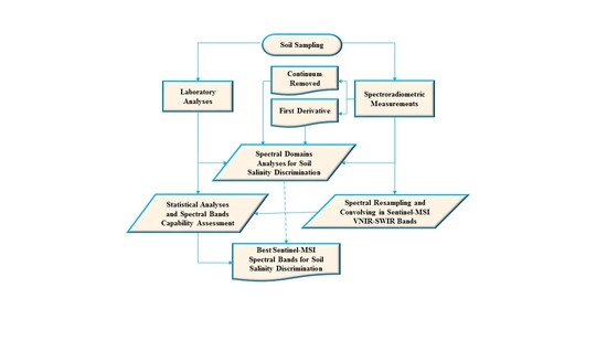
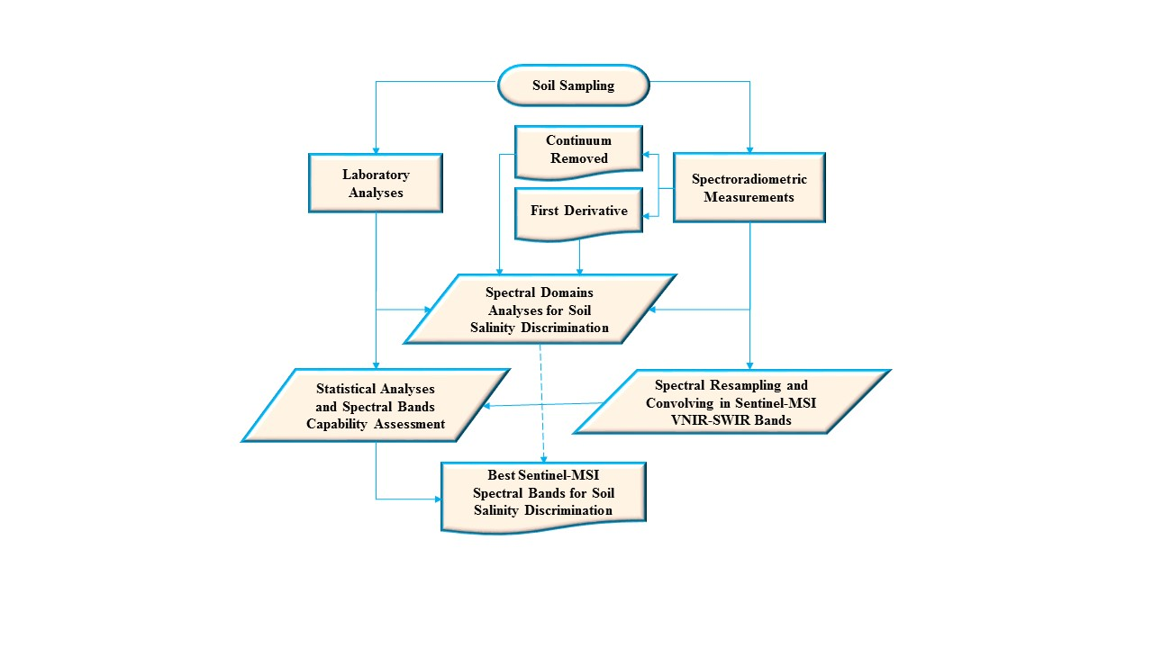
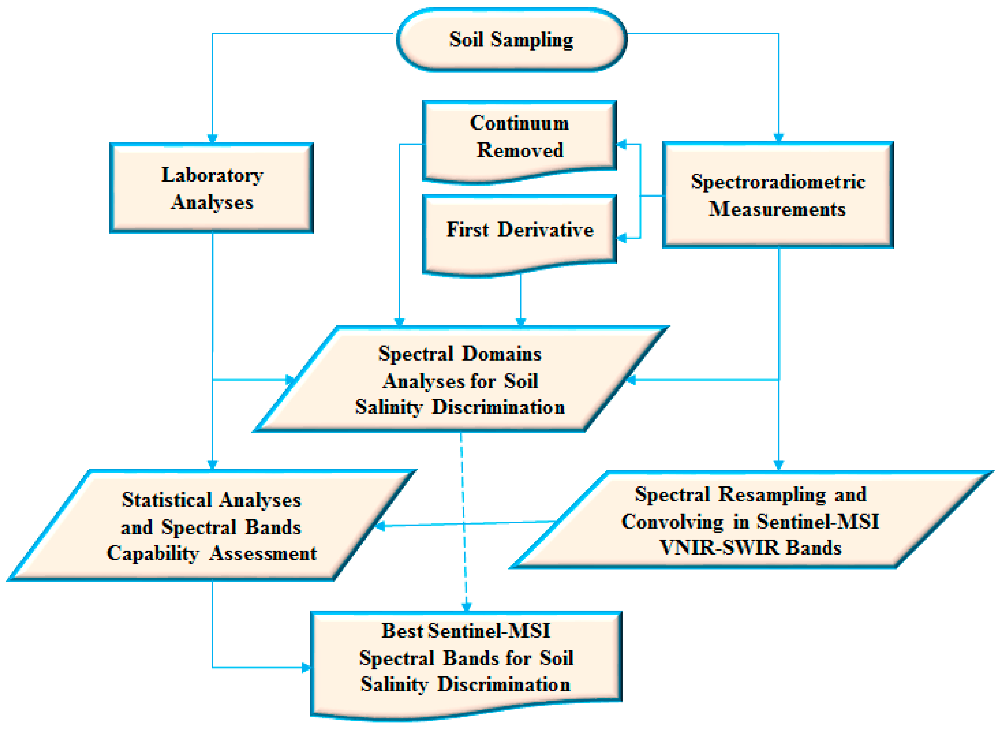
2. Materials and Methods

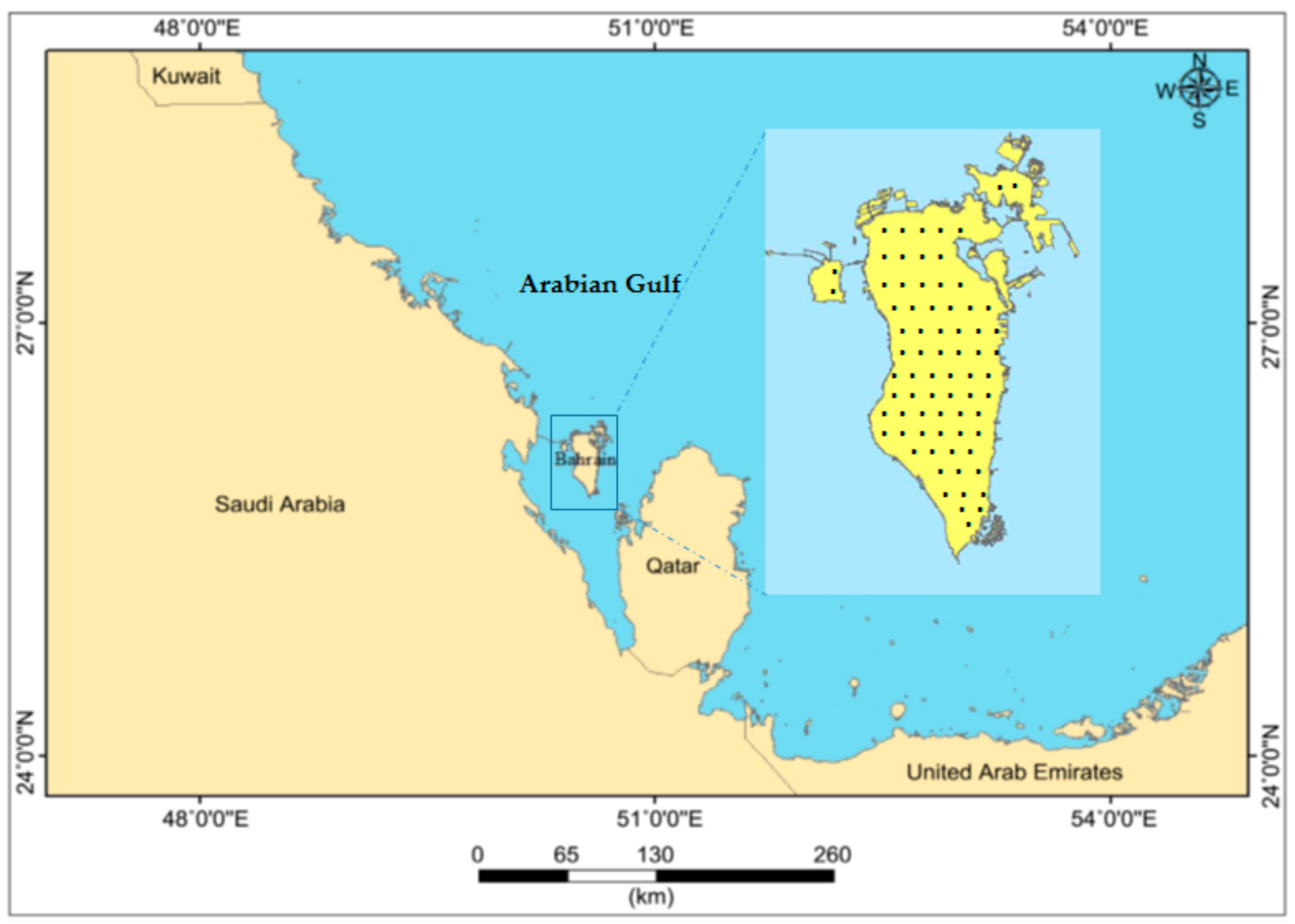
The used methodology is summarized in Figure 1, involving five fundamental steps: (1) A field campaign was organized and a total of 160 soil samples were collected with various salinity levels, from extreme salinity (Sabkha) to non-saline soil (agricultural fields). Observations and remarks about each soil sample were noted, photographed and its geographic location was recorded using GPS; (2) The bidirectional reflectance factor was acquired above each soil sample in a Goniometric-Laboratory using an ASD (Analytical Spectral Devices) FieldSpec-4 high resolution (Hi-Res) spectroradiometer [23]. The spectra of the representative salinity classes were transformed using the continuum-removed reflectance spectrum (CRRS) [24], and the first derivative (FD) [25]. Then, all the measured spectra were resampled and convolved in the solar-reflective spectral bands of Sentinel-MSI sensors using the Canadian Modified Herman transfer radiative code (CAM5S) [26] and the relative spectral response profiles characterizing the filters of each band of MSI; (3) In the laboratory, the soil reaction (pHs), the electrical conductivity (EC-_Lab), and the major soluble cations (Na⁺, K⁺, Ca²⁺+, and Mg²⁺) and anions (CO₃²⁻, HCO₃⁻, Cl⁻, and SO₄²⁻) extracted from a saturated soil paste were measured, as well as the Sodium Adsorption Ratio (SAR) was calculated [27]; (4) These analyses and the field observations relative to each soil sample were used for interpretation and examination of the measured spectra and their transformations (CRRS and FD); (5) Finally, statistical analyses were conducted using second-order polynomial regression (p < 0.05) between the measured EC-_Lab and the resampled and convolved reflectances in the MSI spectral bands were applied to corroborate or to deny which spectral domain and which spectral bands are significant for soil salinity discrimination.

2.1. Study Site

The Kingdom of Bahrain (25°32′ and 26°00′N, 50°20′ and 50°50′E) is an archipelago of 33 islands located in the Arabian Gulf, east of Saudi Arabia and west of Qatar (Figure 2) with a total land area of about 778.40 km². According to the aridity criteria and the great variations in climatic conditions, Bahrain has an arid to extremely arid environment [28]. The climate is characterized by high summer temperatures of an average 45 °C during June-September and an average of approximately 17 °C in winter from December to March. Rain is sparse, and occurs primarily from November to April, with an annual average of 72 mm, sufficient only to support the most drought-resistant desert vegetation. Mean annual relative humidity is over 70% due to the surrounding Arabian Gulf water, and the annual average potential evapotranspiration rate is 2099 mm [29]. Under such climatic conditions, where precipitation is excessively low to maintain a regular percolation of rainwater through the soil, soluble salts are accumulated in the soil, influencing soil properties and environment causing low soil productivity. Indeed, these factors have significant impacts on land degradation, crop production, economic aspects, and infrastructure, as well as ecosystem functionality, human wellbeing, and sustainable development [30]. Geologically, Bahrain is characterized by Eocene and Neocene rocks, which are partly covered by Quaternary sediments and a complex of Pleistocene deposits. The dominant rocks are limestone and dolomitic-limestone with subsidiary marls and shales. The leading structure is the north–south axis of the main dome, with minor cross-folds predominantly tilting from northeast to southwest. The beds are gently inclined towards the coast from the center of the main island. The fringes of Bahrain are covered by more recent marine and Aeolian sand dunes, which were derived from the Arabian land connection across the present Arabian Gulf.

2.2. Soil Sampling and Laboratory Analyses

The soils of Bahrain are characterized by five different classes associated with moderate to shallow depths and are closely related to the terrain geology and geomorphology [31]. The natural Solonchak describes soils with no agricultural activities and retain a high gypsum content (high and very high salinity). Then, there is the cultivated Solonchak soil class, which is located in areas either currently or previously exposed to agricultural activities. The Regosols soil class with moderate salinity is depicted as a mixture of raw minerals as well as the natural Solonchak soils, with the possibility for growing scattered halophytic plants. The miscellaneous land class that is represented by a composition of silts and fine sands with low salinity is suitable for agriculture. Finally, there is the non-saline soil class, which is imported to build artificial islands.

A total of 160 samples were collected during the period from 2 to 7 April 2016, based on the spatial representativeness of the major soil classes as discussed above, and considering various degrees of salinity and the non-saline soil (Figure 2). Samples were collected from the upper layer (0 to 10 cm deep) considering an area about 50 × 50 cm. Observations and remarks about each sample (color, brightness, texture, etc.) were noted. The location of each point was automatically labeled and recorded using a 35-mm digital-camera equipped with a 28-mm lens and accurate GPS survey (σ ≤ ±30 cm) connected in real-time to the GIS database.

The most common and used approaches to determine the degrees of soil salinity and properties include the soil reaction (pHs), the EC-_Lab, and the SAR [4]. After spectroradiometric measurements, which are described below, soil samples were air-dried, crushed, and then sieved to obtain the <2mm fraction. Standard laboratory methods were used to measure the pH. Moreover, the saturation extract collected from saturated soil paste was analyzed for the EC-_Lab, and the major soluble cations (Na⁺, K⁺, Ca²⁺, and Mg²⁺) and anions (CO₃²⁻, HCO₃⁻, Cl⁻, and SO₄²⁻) using standard USDA procedures [27]. The SAR was calculated by computing Na⁺, Ca²⁺+, and Mg²⁺ concentrations (in meq/L) from saturation extract, in the standard equation. The EC-_Lab was used for statistical correlations considering the MSI spectral bands individually.

2.3. Spectroradiometric Measurements

Spectroradiometric measurements were acquired in the goniometric laboratory at the Arabian Gulf University, Kingdom of Bahrain. The bidirectional reflectance spectra were measured above each soil sample using an ASD (Analytical Spectral Devices Inc., Longmont, CO, USA) FieldSpec-4 Hi-Res (high resolution) spectroradiometer [23]. This instrument is equipped with two detectors operating in the VNIR and SWIR, between 350 and 2500 nm. It acquires a continuous spectrum with a 1.4 nm sampling interval from 350 to 1000 nm and a 2 nm interval from 1000 to 2500 nm. The ASD resamples the measurements in 1-nm intervals, which allows the acquisition of 2151 contiguous bands per spectrum. The sensor is characterized by the programming capacity of the integration time, which allows an increase of the signal-to-noise ratio (SNR), as well as stability. The data were acquired at nadir with a field of view (FOV) of 25° and a solar zenith angle of approximately 5° by averaging 40 measurements. The ASD was installed at a height of 60 cm approximately over the target, which makes it possible to observe a surface of approximately 700 cm². A laser beam was used to locate the center of the ASD-FOV. The reflectance factor of each soil sample was calculated by rationing target radiance to the radiance obtained from a calibrated “spectralon panel” in accordance with the method described in [32]. Corrections were made for the wavelength dependence and non-Lambertian behavior of the panel.

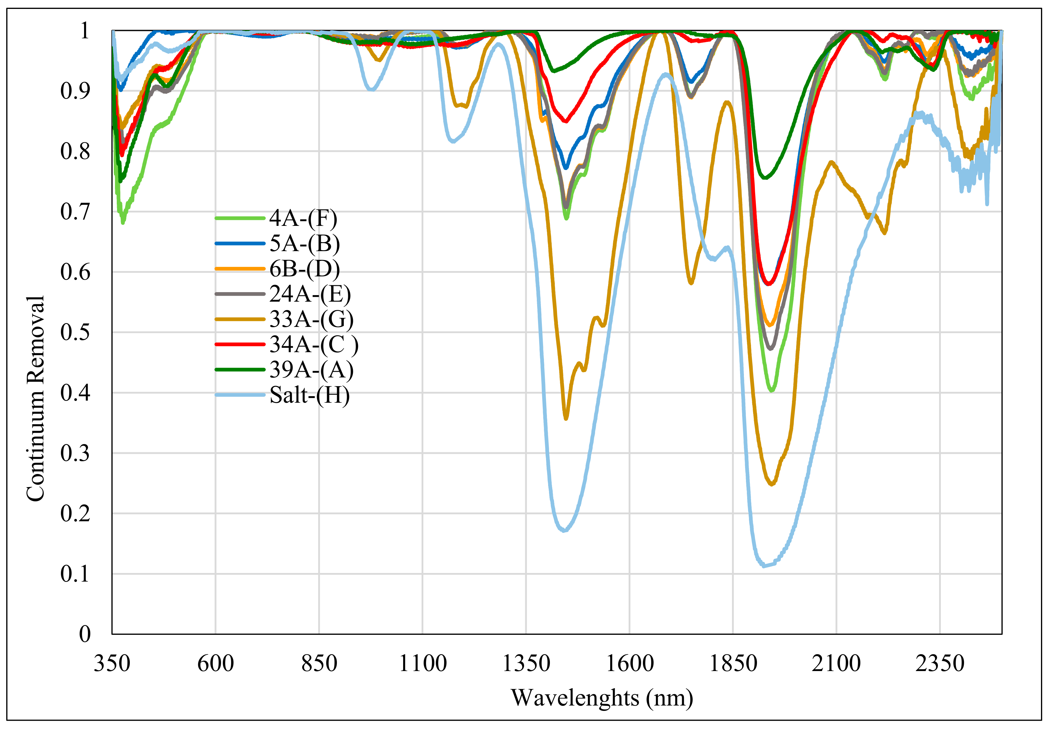
2.4. Continuum-Removed Reflectance Spectrum

Several methods were developed to process spectral signatures to retrieve information regarding the change in reflectance over a specific bandwidth [33,34]. For spectral signatures between 350 and 2500 nm, absorption bands, such as position, depth, width, and asymmetry of the features, were used to quantitatively estimate the mineral or chemical composition of samples from the measured spectra in the field and/or in the laboratory. To enhance these absorption features, many approaches were proposed, such as the relative absorption-band-depth [35], the spectral feature fitting technique [36], and the Tricorder and Tetracorder algorithms [37,38]. These approaches work on so-called CRRS, thus acknowledging that the absorption in a spectrum has two components: a continuum and individual features [24,34,39]. A continuum is a mathematical function used to isolate a particular absorption feature for analysis. It corresponds to a background signal unrelated to specific absorption features of interest [40]. According to Clark et al. [24], CRRS normalizes the original reflectance spectra and helps to compare individual absorption features from a common baseline. The continuum is a convex hull fit over the top of a spectrum under study using straight-line segments that connect local spectra maxima. The first and last spectral data values are on the hull; therefore, the first and last bands in the output continuum-removed data file are equal to 1.0. In other words, after the continuum is removed, a part of the spectrum with no absorption features will have a value of 1, whereas complete absorption (albeit unlikely to actually occur) would be near 0, with most absorptions falling somewhere in between. The spectral continuum can be thought of as what the original spectrum would look like if there were no absorption band. The continuum-removed spectrum is the original spectrum divided by the continuum [40]:

S_cr = (S/C)

(1)

where S_cr is the CRRS, S is the original spectrum, and C is the continuum curve. In this study, the continuum algorithm already developed [24] and implemented in ENVI was used [40].

2.5. First Derivative

The spectral derivative is a powerful mathematical method commonly used in hyperspectral remote sensing data analysis. It reduces the fluctuations, filters the noise (SNR) in the spectral signature, and enhances the more important and significant absorption features related to a specific target (or application). It uses first, or higher, derivatives of absorption bands with respect to the wavelength for qualitative and quantitative analyses [41,42,43]. This process yields helpful features, such as maxima, minima, and points of inflection of the original spectral signature. First derivative (FD) may swing with greater amplitude than the original spectra. For example, a spectrum suddenly changes from a positive to a negative slope, such as at the peak of a narrow feature. The more distinguishable derivatives are especially useful for separating out peaks of overlapping bands [44]. FD is the rate of change of absorption features between 350 and 2500 nm, it starts and finishes at zero. It also passes through zero at the same wavelength as λ_max of the absorption feature. Either side of this point are positive and negative bands with maximum and/or minimum at the same wavelengths as the inflection points in this specific feature. This bipolar function is characteristic of all odd-order derivatives [45]. In this study, FD was implemented in the MATLAB environment [46] using finite approximation to calculate the change in reflectance over a bandwidth Δλ, defined as Δλ = λj − λi, where λj > λi:

$$\frac{d{s}_i}{d{\lambda }_i}=\frac{s\left({\lambda }_j\right)-s\left({\lambda }_i\right)}{\Delta \lambda }$$

(2)

where s is the spectrum used for the derivative transformation.

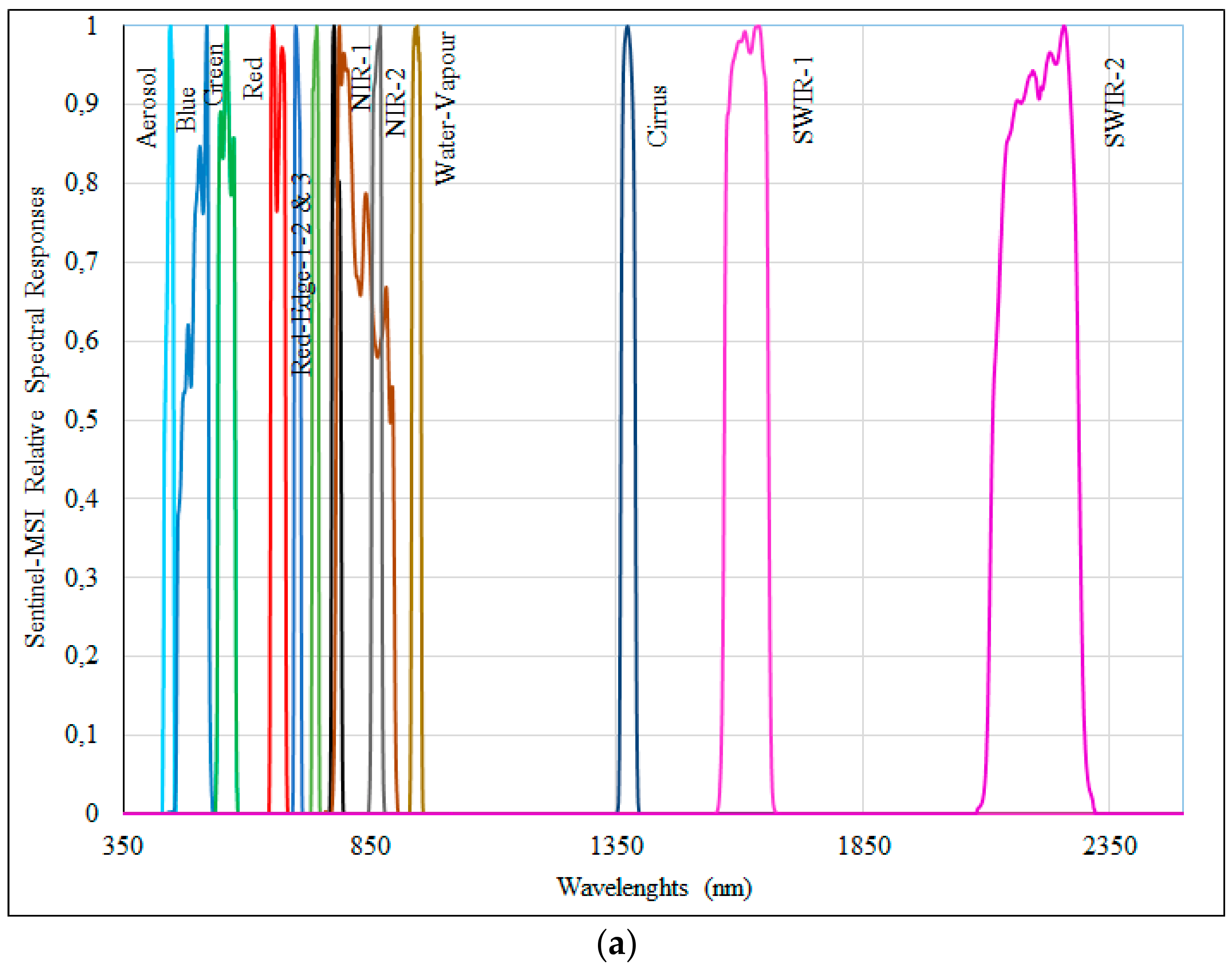
2.6. Sentinel-MSI Simulated Data

The Sentinel-2 satellite was launched on 23 June 2015 with the MSI on board. The synergy between Sentinel-MSI and Landsat-OLI significantly increase the temporal resolution for several environmental and natural resource applications, such as the vigor of vegetation cover, emergency management, soil salinity dynamics, water quality, and climate change impact analysis at local, regional, and global scales. Sentinel-MSI is the result of close collaboration between the European Space Agency, the European Commission, industry, service providers, and data users. The MSI images the Earth’s surface reflectivity with a large field of view in 13 spectral bands in the VNIR and the SWIR at 10, 20, and 60-m pixel sizes. The swath of each Sentinel-MSI scene is 290 km, permitting global coverage of the Earth’s surface every 10 days. The MSI radiometric performance is coded in 12 bits, enabling the image acquisition in 4095 digital numbers, ensuring radiometric accuracy of less than 5% and an excellent signal-to-noise ratio [47].

Table 1. The Sentinel-MSI effective bandwidths.

Spectral Bands	Sentinel-MSI
	λ Centre (nm)	∆λ (nm)	Pixel Size (m)
Coastal-Aerosol	443	20	60
Blue	490	65	10
Green	560	35	10
Red	655	30	10
Red-Edge-1	705	15	20
Red-Edge-2	740	15	20
Red-Edge-3	783	20	20
NIR-1	842	115	10
NIR-2	865	20	20
Water-vapor *	945	20	60
Cirrus *	1375	30	60
SWIR-1	1609	85	20
SWIR-2	2201	187	20

* The cirrus and water vapor bands were note considered in this study.

summarizes the effective bandwidth characteristics for MSI.

The measured bidirectional reflectance factors using the ASD have a 1-nm interval, which allows the acquisition of 2151 contiguous hyperspectral bands per spectrum. However, most multispectral remote sensing sensors measured the reflectance that is integrated over broad bands. Consequently, the measured spectra over each soil sample was resampled and convolved to match the MSI solar-reflective spectral responses characteristics (Figure 3a). In the first step, the resampling procedure considers the nominal width of each spectral band (Table 1). Then, the convolution process was executed using the modified radiative code CAM5S [26]. This fundamental step simulates the signal received by the MSI sensor at the top of the atmosphere from a surface reflecting solar and sky irradiance at sea level considering the relative spectral response profiles characterizing the filters of each sensor band (Figure 3a), and assuming ideal atmospheric conditions without scattering and absorption. Considering the 160 soil samples, these simulated reflectances in each spectral band of the MSI were fitted with the salt content measured in the laboratory (EC-_Lab) using second regression analyses (p < 0.05). In addition to CRRS and FD, such a statistical examination step was used to evaluate the strength of the relationship (correlation coefficient) between the EC-_Lab and the reflectances in each Sentinel-MSI band, i.e., the measurement of the sensitivity of each spectral band and its capability to discriminate among various salt-affected classes.

3. Results and Discussion

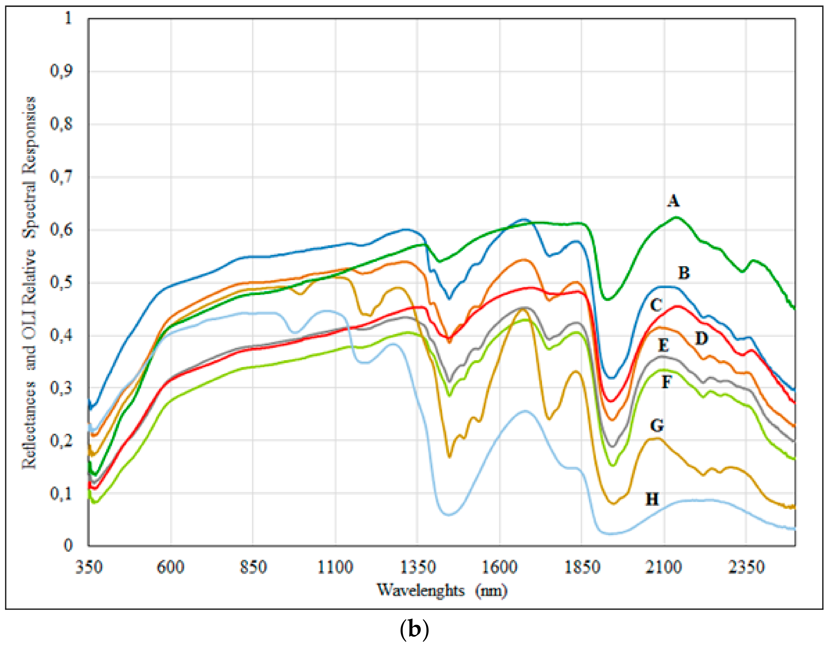
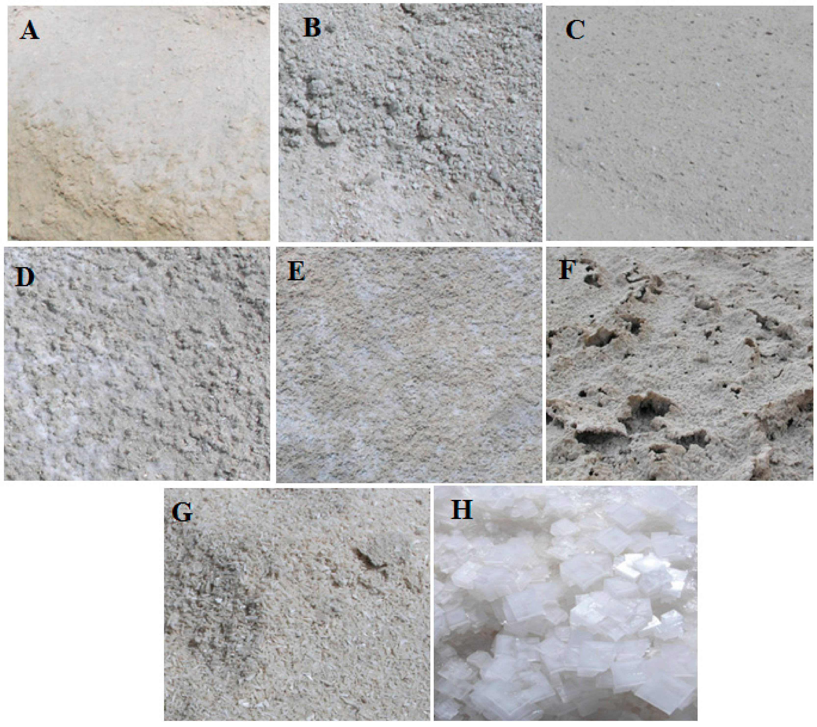
3.1. Spectral and Laboratory Analyses

Globally, the spectral signatures of the 160 considered soil samples are controlled by the type of salt existing in each soil sample, such as sulfates, chlorides, and/or carbonates. The results showed different amplitudes and several absorption features depending on the chemical compositions and the mineralogy of the existing salts in the selected soil samples. Moreover, the spectral signatures are also influenced by several factors, such as mineralogical composition, impurity, structure, and texture of the soil and salt crystals, and the soil optical properties (color brightness, roughness, organic matter, moisture, etc.). Furthermore, the laboratory analyses of all soil samples revealed that the EC-_Lab values are distributed in a wider range, between 2.6 and 850 dS/m. The lowest values represent the samples of agricultural fields, while the highest indicated the Sabkha, which is pure salt. The pH is ranging from neutral to very strongly alkaline, between 7.09 and 8.59. Overall, the laboratory analyses showed that the solution chemistry was dominated by cations (Na⁺ > Ca²⁺ + Mg²⁺ > K⁺) and anions (Cl⁻ > SO₄²⁻ > HCO₃⁻); CO₃²⁻ was undetectable. The trend showed a very high concentration of sodium (Na⁺), which generally exceeds the sum of both calcium (Ca²⁺) and magnesium (Mg²⁺), in addition to dominant chloride (Cl⁻), which exceeds sulfate (SO₄²). Sodium exhibited the highest concentration due to the greater solubility of Na⁺ salts in the saturated paste compared to other minerals. This was reflected in the high SAR values ranging between 6 and 1094 (mmoles/L)^0.5.

To facilitate the spectral analyses and presentation, the 160 soil samples were classified into eight significant and representative classes based on the spectral signatures behavior and the results of the chemical laboratory analyses results. Figure 4 illustrates the photos that represent these eight nominated classes, and

Table 2. Description of the eight considered soil-salinity samples.

Sample	Munsell Color	Standard Color	Texture	Remarks
A	10YR 7/6	Yellow	Sandy	Sandy soil without gypsum and shells
B	10YR 8/1	White	Sandy-Clay-Loam	With small amount of gypsum crystals and shells
C	10YR 7/2	Light-gray	Loamy-Sandy	Sandy soil with small amount of gypsum crystals and shells
D	10YR 7/2	Light-gray	Sandy-Loam	Beginning of salt crust formation. Small amount of gypsum crystals and shells
E	10YR 7/2	Light-gray	Sandy-Clay-Loam	Beginning of salt crust formation. Small amount of gypsum crystals and shells
F	10YR 7/2	Light-gray	Sandy-Clay-Loam	Crust of salt with gypsum, calcium carbonate, and small amount of shells
G	5Y 8/1	White	Sandy	Pure gypsum crystal deposited by wind erosion
H	10YR 8/1	White	Pure salt (halite)	Sabkha

summarizes their characteristics descriptions. The textures represent a mixture of sand, loamy-sand, gypsum, calcium carbonate, small amount of shells, and pure salt. Figure 3 illustrates their spectral signatures and the relative spectral response profiles characterizing the filters of MSI and the position of each spectral band in the electromagnetic spectrum. To carefully analyze these spectra according to the salt mineralogy, it should be considered that gypsum reveals significant absorption features at 1000, 1210, 1450, 1490, 1540, 1748, 1780, 1945, 1975, 2175, 2215, 2265, and 2496 nm. Strong water absorption features characterize four of them (975, 1190, 1450, and 1945 nm), and only three weak bands near 1350, 1800, and 2208 nm were observed (atmospheric water vapor absorption features at 1440 and 1920 nm are note considered in this analysis). These observations corroborate findings of other studies [48,49,50,51]. For the halite (NaCl), several absorption features are also manifested in the SWIR region (980, 1190, 1450, 1800, and 1950 nm). However, several authors reported the halite absorption features at 1400, 1900, and 2250 nm [6,50,51], halite and sylvite at 1440 and 1933 nm, and bischofite (MgCl₂·6H₂O) at 1190 and 1824 nm. These specific absorption features are identified accurately in controlled environment and for a specific contiguous hyperspectral wavebands in nm. This situation is different and more complicated in the real world using multispectral broadband because variations in the soil reflectance cannot be attributed to a single and unique salt type or soil property within individual pixels of 100, 400, or 900 m². In addition, depending on the positions of the bands in the electromagnetic spectrum, each sensor collects the electromagnetic radiation that is reflected by salt-affected soil differently. According to this preliminary analysis, these spectral signatures illustrate clearly that the saline soil or the salt-crusts exhibit narrow diagnostic absorption features, particularly in the SWIR region, 1000 to 2500 nm. However, the reflectance changed proportionally as the salt concentrations increased in the soil samples from 26 to 507 dS/m (

Table 3. Laboratory determination of EC-_Lab, pH, and ion content of the eight selected soil samples that are presented in Figure 3 and Figure 4.

Sample	pH	EC-Lab	Cl−	HCO3−	SO4−2	Ca2+	K+	Mg2+	Na+	SAR (mmoles/L)0.5
			(mg/L)			(mg/L)
A	8.33	26.0	9567.5	305.1	4624.7	563.6	367.6	558.2	6599.4	46.9
B	8.10	55.6	23,209.9	305.1	6771.7	392.5	697.2	1247.9	15,164.8	84.5
C	7.71	119.6	56,341.7	305.1	30,495.2	1787.8	1132.9	2327.9	44,057.0	162.0
D	7.47	195.3	120,833.4	305.1	27,527.6	2056.0	1840.0	4484.8	79,607.6	225.9
E	7.57	333.0	142,094.4	305.1	6696.6	1342.3	1236.1	2487.4	86,990.4	325.2
F	7.35	406.5	185,325.1	305.1	68,488.8	1580.3	3105.0	4643.2	140,500.0	403.6
G	7.60	445.5	135,716.1	610.2	1700.0	1128.1	843.4	1239.7	84,795.9	415.2
H	7.60	507.0	142,803.1	610.2	17,107.4	1227.2	1644.9	1399.0	95,860.0	444.7

). This observation is consistent with many other studies indicating the importance of the spectral domain between 1200 and 2500 nm for soil salinity characterization [18,52,53,54].

Otherwise, in the VNIR region, the spectra of the selected eight soil classes with different salt content showed a severe confusion caused by the soil optical properties (i.e., color, brightness, texture, etc.) dominating the signal in this spectral region. For example, the spectra of the sample “D” (195 dS/m) coincide with that of sample “H” (507 dS/m), although they do not have the same EC-_Lab values, because the soil characteristics play a fundamental role in this confusion (Figure 3b and Table 3). In fact, sample “D” is a sandy soil characterized by small amount of gypsum crystals and shells, and the beginning of salt crust formation (light gray and white color, 10YR 7/2), while sample “H” is a pure salt-sabkha (white color, 10YR 8/1). Similar confusion is observed between the opposite sample classes “A” and “H”, respectively, with 26 and 507 dS/m EC-_Lab values. Moreover, the samples “A” and “G” are sandy soils with EC-_Lab of 26 and 445.5 dS/m, respectively; however, these two samples exhibited approximately the same spectral behavior and amplitude in the VNIR according to their color (Figure 3b and Table 3). Consequently, the separation between “D” and “H” or “A” and “G” samples in the VNIR, in general, could not be applied, especially in the coastal and blue bands. However, Figure 3b shows that the increase of EC-_Lab values synchronize with the significant variation among the salt-affected soil spectra, and progressively from the 1000 to 2500 nm portion of the spectrum. For instance, in this SWIR domain, from “A” to “H” soil samples, the spectra changed progressively in amplitude and shape as a function of EC-_Lab (from 26 to 507 dS/m, see Table 3), as well as a function of SAR (from 46.9 to 444.7 (mmoles/l)^0.5). The observed ambiguity between “D” and “H” or “A” and “G” samples in the VNIR, is completely dismissed in the SWIR and it is easy to see gradually the spectral signature position of each sample according to its EC-_Lab content. Definitely, the Sentinel-MSI SWIR-1 and SWIR-2 bands show the highest potential to efficiently discriminate among different degrees of salinity in the soil (Figure 3b). These findings corroborate the results of other studies characterized several soils rich in sulfate minerals, carbonates, and bicarbonates, sodium chloride, etc., in the SWIR regions [1,6,14,15,48,50,51,55,56].

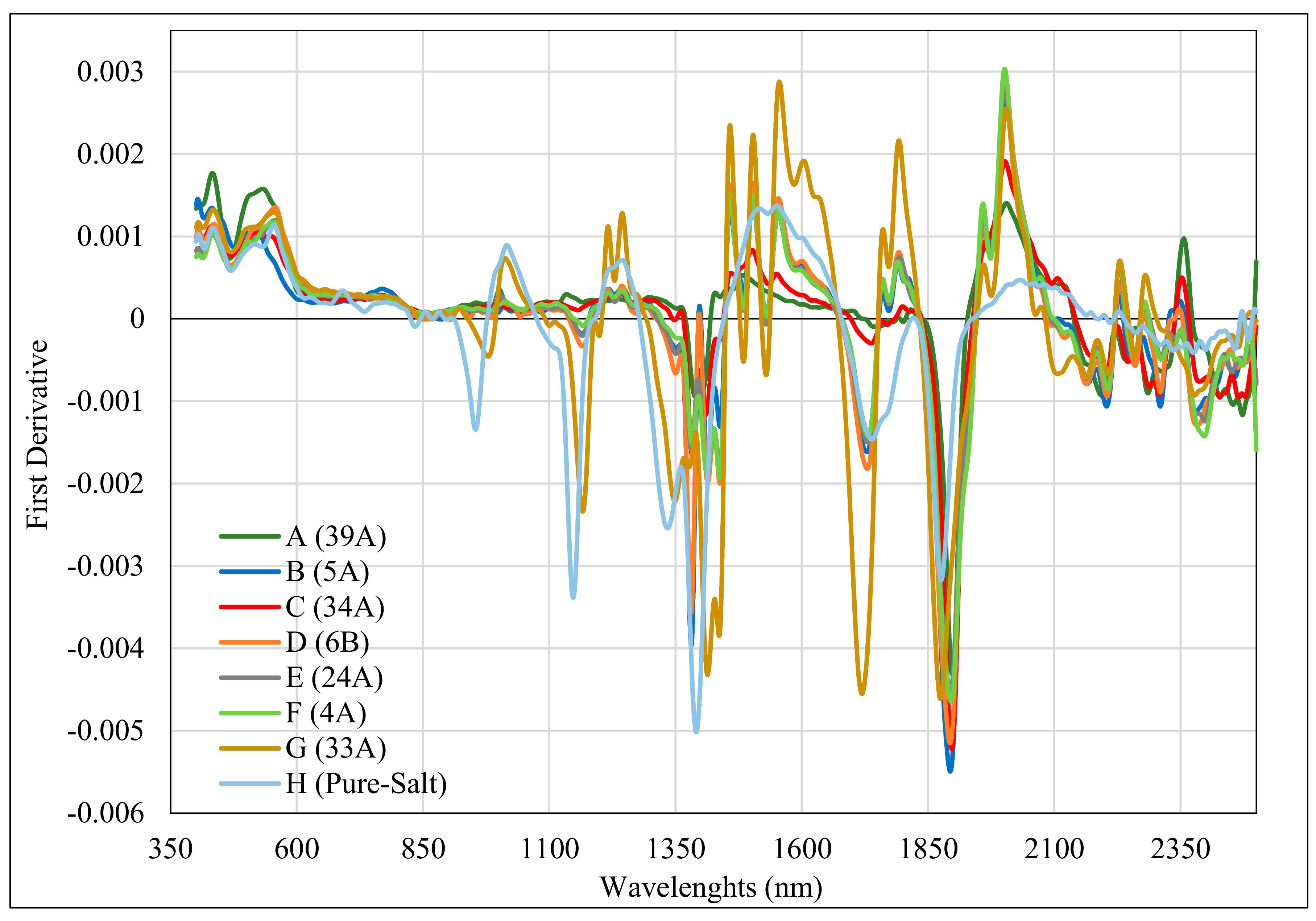
3.2. CRRS and FD Analyses

The derived CRRS of the eight considered soil samples are illustrated in Figure 5. The spectral transformation shows a total absence of absorption features between 525 and 935 nm, but revealed some features between 350 and 525 nm, and enhanced numerous and significant absorption bands between 935 and 2500 nm (i.e., absorption features beyond 1350 nm were broadened). In such spectral regions, the CRRS has shown that increases of salt in the soil (EC-_Lab) induced automatic changes in the depth of absorption features, particularly in the water absorption bands, which were shifted toward shorter wavelengths. Consistent absorption features are observed at wavelengths of 980, 1175, 1448, 1933, and 2430 nm, particularly for the pure salt sample (sodium chloride). Apparently, these absorption peaks increase progressively as the salinity content increased in the soil sample. These results of transformations are compatible with those obtained by Farifteh [51]. Furthermore, the revealed bands between 350 and 525 nm are not conclusive, unfortunately, because the increase in salinity content was found to be at a level that does not represent significant and separate features among soil salinity classes. Indeed, in this specific electromagnetic window (coastal and blue bands) the sample “H” which is 10 time more saline than the sample “B” (respectively EC-_Lab of 507.0 and 50.5 dS/m) are showed similar absorption features. Moreover, the samples “A”, “C”, and “E” with different salinity contents (EC-_Lab of 26.2, 90.0 and 381.0 dS/m, respectively) presented comparable absorption features (Figure 5). This similarity is automatically related to the color and the brightness of the soil samples rather than salinity content degrees. In fact, “B” and “H” samples have the same color (white, 10YR 8/1), while the samples “A”, “C”, and “E” are characterized by mixed color and brightness: white-beige, light-gray, and light-gray-white (Table 2). Therefore, the CRRS analysis corroborates the original spectral signature behavior that the Sentinel-MSI SWIR spectral domains are more suitable for soil salinity discrimination.

Figure 6 illustrates the FD of reflectance spectra of the eight soil-salinity classes (Table 2). The results revealed that the FD enhances two absorption bands at 415 and 470 nm, as well as various features between 950 and 2500 nm. In addition, the absorption features of soil minerals broaden considerably when the absorbed moisture varies. However, it is very difficult to make a clear distinction and separation among many absorption bands comparatively to CRRS. It looks that the FD can detect small concentrations of soil constituents as it depends on the shape of the characteristic absorption features, but not on the depth. Conversely, these features become more ambiguous due to water content. These observations are consistent with the findings pointed out by other studies [56,57]. Nevertheless, CRRS transformation provides globally better results in comparison with the FD processing, since it is less susceptible to random variability in the spectra as reported earlier [58]. Although the FD is not able to identify the best absorption features for salt-affected soil discrimination, as it seems to be minimizing the effect of multiple scattering due to particle size [59] and provide an overall, but comprehensive, message that the SWIR regions are better than the VNIR for soil salinity discrimination.

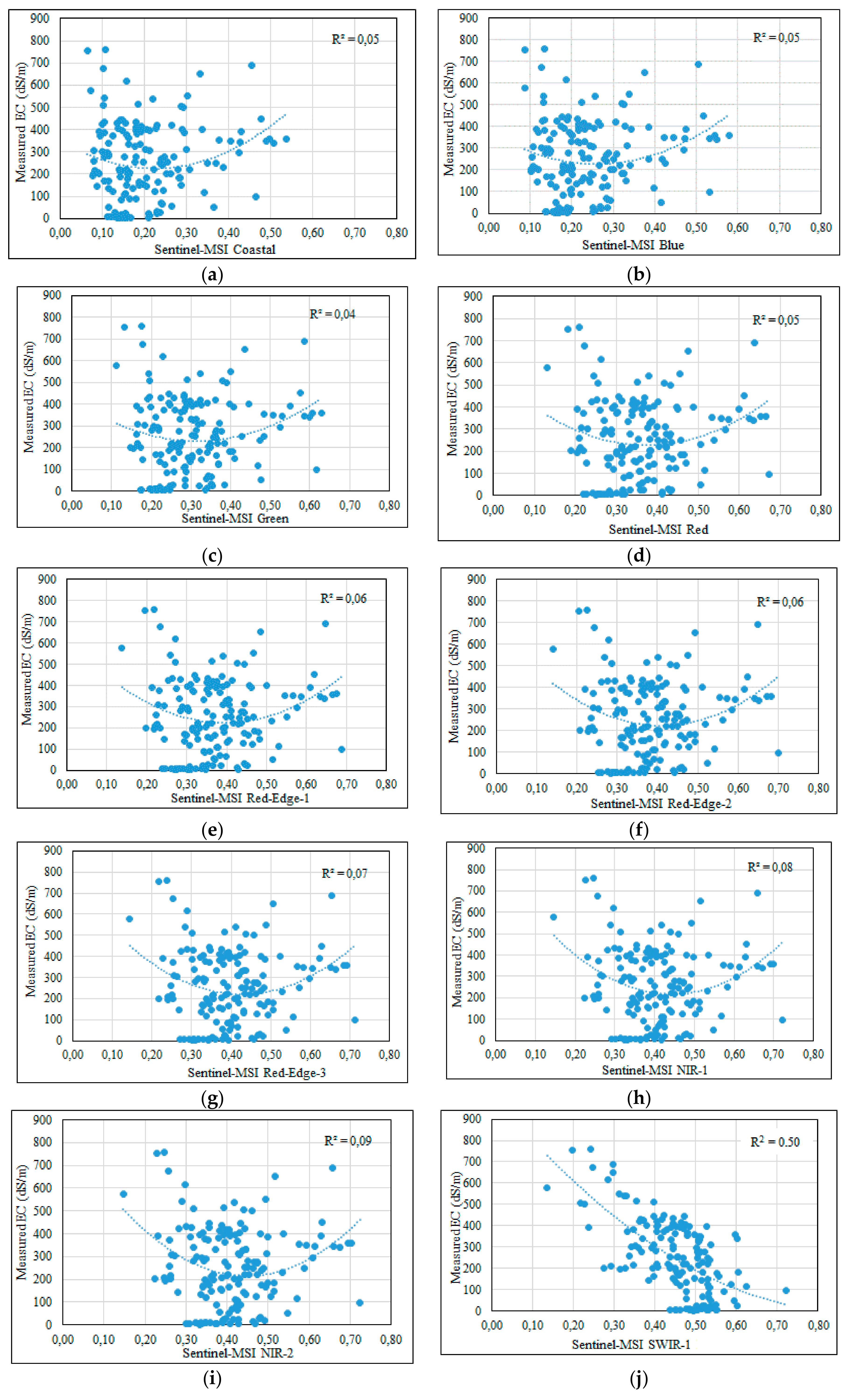
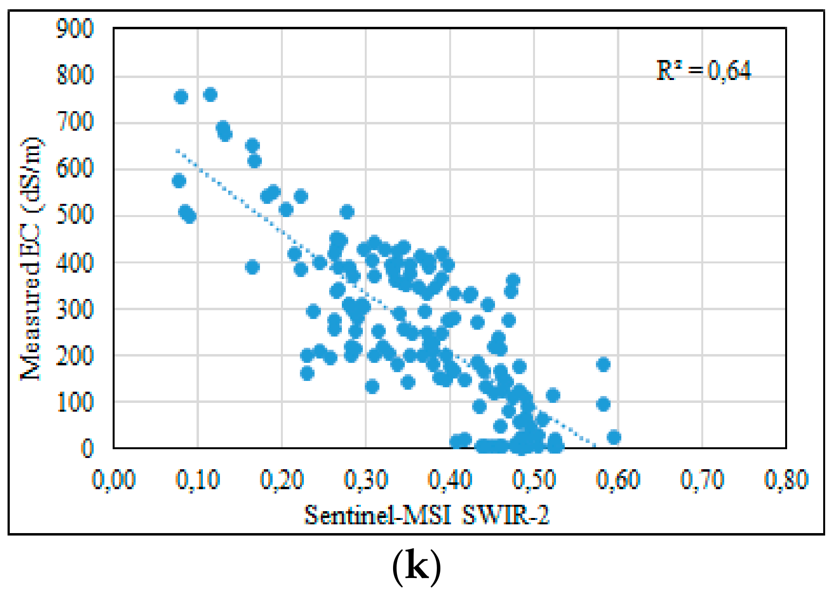
3.3. Statistical Analysis between EC-_Lab and Spectral Bands of MSI

Considering the 160 soil samples, several statistical functions were fitted between the measured EC-_Lab content and the resampled and convolved reflectances in the VNIR and SWIR bands of the MSI sensor. A second-order polynomial regression (p ≤ 0.05) allowed the best fit. Obtained results showed that the reflectances in the four visible bands (coastal, blue, green, and red) are insignificantly correlated (R² ≤ 0.05) with the salt content in the soil (Figure 7a–d). These very low correlations are also achieved in the red-edge (R² ≤ 0.07) and in the NIR (R² ≤ 0.09) spectral bands (Figure 7e–i). Indeed, the regressions presented in Figure 7a–i illustrate that, independently of the salt-content, the 160 sampled points are scattered randomly without any trend or substantial relationship between these bands’ reflectances and the EC-_Lab. The statistical results corroborate the previous spectral signatures and their transformation (CRRS and FD) analyses indicate that the Sentinel-MSI VNIR spectral bands are not appropriate and not consistent for correct and accurate discrimination among various soil salinity classes in arid landscape. Moreover, these findings are consistent with Nawar et al. [13,60], which concluded that the visible bands of ETM+ and ASTER have the lowest contribution to estimate soil salinity comparatively to the other spectral bands. Additionally, recently Rahmati and Hamzehpour [19] revealed that no significant correlation (R² ≤ 0.03) exists between the measured EC-_Lab and the reflectance in the visible bands of ETM+ sensor. Contrarily, the Sentinel-MSI SWIR bands 1 and 2 have the highest power for soil salinity discrimination with an R² of 0.50 and 0.64, respectively (Figure 7g,k), which are consistent with several other studies that showed the potential of these spectral wavebands of OLI, ALI EO-1, and WorldView-3 sensors for salt-affected soil discrimination [14,15,61,62]. According to Nawar et al. [60], the SWIR bands of ASTER, especially bands 9, 8, and 7 exhibited the highest contribution for soil salinity estimation. Moreover, another study [19] indicated that the SWIR bands of the ETM+ sensor increases the accuracy of the soil salinity prediction, whereas several other studies exploring hyperspectral remote sensing showed that the bands within the SWIR regions are the best for evaluating the soil salinity [59,63,64].

3.4. Discussion

The multispectral remote sensing such as Sentinel-MSI or Landsat sensors series are the most used technology to investigate the soil salinity detection and mapping. However, the broad bands of these sensors lack the necessary sensitivity for precise quantification and discrimination of the varying degrees of salinity in the soil particularly in the VNIR spectral domain. In such wavelengths, the main factors affecting the salt-affected soil spectral signatures are represented by salt types, soil mineralogy, level of moisture, organic matter content, color and brightness, roughness, and vegetation cover. Obviously, these factors influence the signal gathered by the sensor in a specific pixel size causing severe confusion between the salt in the soils and the soil optical properties as demonstrated in the present study for Sentinel-MSI using four independent analyses (spectral signatures, CRRS, FD, and statistics). Moreover, using other sensors such as TM and SPOT-HRV, has been reported [9] that spectral confusion occurs in the VNIR bands between saline areas and desertified regions in Egypt. Spectral confusion was also problematic, as pointed out in a study carried out by Verma et al. [7] in which salinity was mapped in certain regions of India using TM demonstrating the difficulty to highlight the difference between affected soils and fallow fields. During the attempts made by Metternicht [65] and Metternicht and Zinck [2,8] to differentiate between different levels of soil salinity in Australia, the results revealed that spectral confusion occurs especially in the VNIR spectral domain. Likewise, using multispectral field measurements, Metternicht and Zinck [1] found spectral confusions between salt crust and bright silt-loam textural crust, especially in the blue and green spectral bands. Indeed, the surface brightness due to high silt content provides higher reflectance than the salty crust, but normally non-saline crusts must have lower reflectance and a different spectral signature than the salt crust. Hawari [50] and Farifteh [51] demonstrated the absence of the salt absorption features in the VNIR domain in analyzing the spectral signatures of several types of salt minerals group (sulfate, carbonate, borax, and halite).

Furthermore, the results of the proposed processing methods (spectra, CRRS, FD, and statistical fits) confirmed the same conclusions that the SWIR regions, particularly the Sentinel-MSI SWIR-1 and SWIR-2 bands, have the best potential for saline soils detection and discrimination. This finding is attributed to the chemical composition and the mineralogy of the salt in the soils control significantly the behavior of their spectral signatures generally in the SWIR wavelengths. In addition, in these spectral regions the artefacts of soil optical properties are absent or insignificant. Thus, the findings of the present study consistent with other studies that have been conducted in the field, laboratory, and using real satellite data acquired with several sensors, such as TM, ETM+, OLI, ALI EO-1, and WorldView-3. Chapman et al. [66] showed that the SWIR bands of TM provide excellent discrimination of evaporite mineral zones in salt flats. Moreover, Drake [53] described the various absorption peaks of the salts found in evaporite minerals in the SWIR wavelengths. The study undertaken by Hawari [50] showed that the absorption features between 1000 and 2500 nm are consistent with the detection of the gypsum, halite, calcium carbonate, and sodium bicarbonate. Other studies focused on direct observations of bare soils with different types of saline crusts and indirect observations of vegetation cover confirmed that bands found in the SWIR were associated with information related to salt content differences and provided some information on salt types [6,48,49,59,67,68]. Nawar et al. [13] demonstrated that salt-affected soils exhibit two deep absorption features at 1415 and 1915 nm, and have several weak absorption features near 1748, 2207, and 2385 nm. The study reported that on global scale, the spectral signature amplitude decreases significantly with the level of soil salinity, especially in the SWIR domain. Shrestha [69] concluded that the SWIR band was the most correlated with soil salinity by comparing the six bands of ETM+. Using ALI EO-1, OLI and WorldView-3 sensors, Bannari et al. [14,15,61,62] found that the SWIR bands of these sensors offers the best potential for soil salinity detection in irrigated agricultural lands in North Africa, as well in the arid lands in the Middle East. Moreover, Leone et al. [70], Odeh and Onus [71], and Zhang et al. [72] demonstrated that the SWIR bands could be used for soil salinity estimation in agricultural fields better than other spectral domains. According to Fan et al. [73], spectral indices operating in the VNIR of ETM+ sensor are negatively related to soil salinity discrimination; however, the indices based on the SWIR showed a positive correlation.

In spite of the results obtained in this study, and all notable international works mentioned above that suggested the bands within the SWIR wavelengths for soil salinity modeling and mapping, other users of remote sensing advocated the importance of the VNIR bands. Indeed, Fan et al. [73] estimated the soil salinity from the ALI EO-1 convolved field spectra in the Yellow River Delta in China, and emphasized the importance of ALI blue and NIR bands for soil salinity discrimination. Madani [74] found a strong relationship between soil salinity and all TM spectral bands, except the two SWIR bands that were non-significant. Moreover, El-Harti et al. [75] found that the association of the OLI coastal band with OLI VNIR bands is a good indicator for spatiotemporal monitoring of soil salinization in irrigated agricultural lands. Likewise, Bai et al. [76] demonstrated that only the “magic” blue band of the OLI sensor contributed significantly to soil salinity prediction. Contrariwise, Mashimbye [59] indicated that the coastal band is more sensitive to the alkalinity (pH) than to the electrical conductivity (EC-_Lab). However, as demonstrated in this study and reported by Metternicht and Zinck [1], the blue and the coastal bands are very sensitive to the soil optical properties characteristics and variation (color, brightness, texture, etc.), which seems to be of limited contribution to discriminate among salt-affected soil classes. In addition, it could be concluded that these wavelengths are very sensitive to atmospheric scattering by tiny bits of dust and water vapor in the air, and even by air molecules, than the longer wavelengths [77]. Nevertheless, during the conceptualization of most optical remote sensing sensors, such as Sentinel-MSI, Landsat-OLI, or any other optical sensor, the spectral domains of coastal and blue are dedicated especially for two specific applications, including shallow water and tracking fine particles, like dust and smoke in the atmosphere [77]. Obviously, for remote sensing scientists and not for those who use remote sensing as a tool, the goal of these two spectral bands is not concerned with the soil mineralogy detection or quantification. Certainly, mapping soil salinity without consideration of the concepts and theory of spectroradiometry and remote sensing sciences will not make the proper choice of the appropriate spectral bands for the soil salinity model exploiting the new generation of remote sensing sensors.

4. Conclusions

This research focused on the potential and the limit of the VNIR and the SWIR spectral bands of MSI sensor on board of Sentinel-2 for soil salinity discrimination and distinction in an arid landscape. The spectral signatures of 160 soil samples with different degrees of salinity and non-saline soil were measured and transformed using CRRS and FD methods. Then, the measured spectra of all considered soil samples were resampled and convolved in the spectral bands of MSI sensor using the Canadian Modified Herman transfer radiative code and the relative spectral response profiles characterizing the Sentinel-MSI band filters. Subsequently, statistical fits were established between the measured electrical conductivity in the laboratory (EC-_Lab) and the resampled and convolved reflectances in the VNIR and the SWIR bands of MSI sensor. Results showed that the salt-affected soil signal measured and convolved in the Sentinel-MSI bands is controlled not only by the salt content existing in the soil, but also by the soil mineralogical composition and optical properties (color, brightness, texture, roughness, etc.), particularly in the VNIR wavelengths. Indeed, spectral signatures exhibited a serious spectral-signal confusion among non-saline and saline-soil samples, as well the CRRS and the FD transformations highlighted this confusion especially in the VNIR bands. The statistical analyses corroborated this limitation indicating that the EC-_Lab and the reflectances in the visible bands (coastal, blue, green, and red) are non-significantly correlated (R² ≤ 0.05). These very low correlations are also obtained in the red-edge (R² ≤ 0.07) and in the NIR (R² ≤ 0.09) bands. Contrariwise, when the EC-_Lab and the SAR values were increased in the soil, the spectral signatures were changed progressively and significantly in amplitude and shape, particularly in the SWIR region (from 1000 to 2500 nm portion of the spectrum). Definitely, the position of the Sentinel-MSI relative spectral response profiles (characterizing the filters of each spectral band) in the spectral signatures showed the potential of the SWIR-1 and SWIR-2 bands to separate efficiently among different degrees of salinity in the soil. Likewise, the CRRS and FD processing stressed the independence of the SWIR domain vis-a-vis the soil artifacts, and corroborated its capability to differentiate significantly among several soil salinity classes. Moreover, statistical fits confirm the effectiveness of Sentinel-MSI SWIR-1 and SWIR-2 band potential for soil salinity classes’ prediction with a significant correlation (R² of 0.50 and 0.64, respectively). Undoubtedly, the synergy between these two bands of Sentinel-MSI and their homologues in Landsat-OLI, which constitute a continuous record of the Earth’s surface reflectivity from space using the Landsat sensor series since 1972, will significantly increase the temporal resolution for soil salinity dynamic monitoring at the global, regional, and local scales.

References

1. Metternicht, G.; Zinck, J.A. Remote Sensing of Soil Salinization: Impact on Land Management; CRC Press Taylor and Francis Group: Boca Raton, FL, USA, 2009; 374p. [Google Scholar]
2. Metternicht, G.I.; Zinck, J.A. Remote sensing of soil salinity: Potentials and constraints. Remote Sens. Environ. 2003, 85, 1–20. [Google Scholar] [CrossRef]
3. Smedema, L.K. Salinity control in irrigated land: Use of remote sensing techniques in irrigation and drainage. In Proceedings of the Expert Consultation, Session 3—Drainage and Salinity Monitoring and Control, Montpellier, France, 2–4 November 1993; FAO, Water Reports 4. pp. 141–150. [Google Scholar]
4. Zhang, H.; Schroder, J.L.; Pittman, J.J.; Wang, J.J.; Payton, M.E. Soil Salinity Using Saturated Paste and 1:1 Soil to Water Extracts. Soil Sci. Soc. Am. J. 2005, 69, 1146–1151. [Google Scholar] [CrossRef]
5. Norman, C.P.; Lyle, C.W.; Heuperman, A.F.; Poulton, D. Tragowel Plains—Challenge of the Plains. In Tragowel Plains Salinity Management Plan, Soil Salinity Survey, Tragowel Plains Subregional Working Group; Victorian Department of Agriculture: Melbourne, Australia, 1989; pp. 49–89. [Google Scholar]
6. Mougenot, B.; Pouget, M.; Epema, G. Remote sensing of salt affected soils. Remote Sens. Rev. 1994, 7, 241–259. [Google Scholar] [CrossRef]
7. Verma, K.S.; Saxena, R.K.; Barthwal, A.K.; Deshmukh, S.N. Remote sensing technique for mapping salt affected soils. Int. J. Remote Sens. 1994, 15, 1901–1914. [Google Scholar] [CrossRef]
8. Metternicht, G.I.; Zinck, J.A. Spatial discrimination of salt- and sodium-affected soil surfaces. Int. J. Remote Sens. 1997, 18, 2571–2586. [Google Scholar] [CrossRef]
9. Hashem, M.; El-Khattib, N.; El-Mowelhi, M.; Abd El-Salam, A. Desertification and land degradation using high resolution satellite data in the Nile Delta, Egypt. In Proceedings of the IGARSS-1997, Singapore, 3–8 August 1997; pp. 197–199. [Google Scholar]
10. Goosens, R.; El Badawi, M.; Ghabour, T.; De Dapper, M. A simulated model to monitor the soil salinity in irrigated arable land in arid areas based upon remote sensing and GIS. EARSeL Adv. Remote Sens. 1998, 2, 165–171. [Google Scholar]
11. Ben-Dor, E.; Metternicht, G.; Goldshleger, N.; Mor, E.; Mirlas, V.; Basson, U. Review of Remote Sensing-Based Methods to Assess Soil Salinity. In Remote Sensing of Soil Salinization: Impact on Land Management; Metternicht, G., Zinck, J.A., Eds.; CRC Press Taylor and Francis Group: Boca Raton, FL, USA, 2009; Chapter 13; pp. 39–60. [Google Scholar]
12. Allbed, A.; Kumar, L.; Sinha, P. Mapping and Modelling Spatial Variation in Soil Salinity in the Al Hassa Oasis Based on Remote Sensing Indicators and Regression Techniques. Remote Sens. 2014, 6, 1137–1157. [Google Scholar] [CrossRef] [Green Version]
13. Nawar, S.; Buddenbaum, H.; Hill, J.; Kozak, J. Modeling and Mapping of Soil Salinity with Reflectance Spectroscopy and Landsat Data Using Two Quantitative Methods (PLSR and MARS). Remote Sens. 2014, 6, 10813–10834. [Google Scholar] [CrossRef] [Green Version]
14. Bannari, A.; Guedon, A.M.; El-Harti, A.; Cherkaoui, F.Z.; El-Ghmari, A. Characterization of Slight and Moderate Saline and Sodic Soils in Irrigated Agricultural Land Using Simulated Data of ALI (EO-1) Sensor. Commun. Soil Sci. Plant Anal. 2008, 39, 2795–2811. [Google Scholar] [CrossRef]
15. Bannari, A.; Guedon, A.M.; El-Ghmari, A. Mapping Slight and Moderate Saline Soils in Irrigated Agricultural Land Using Advanced Land Imager Sensor (EO-1) Data and Semi-Empirical Models. Commun. Soil Sci. Plant Anal. 2016, 47, 1883–1906. [Google Scholar] [CrossRef]
16. Scudiero, E.; Skaggs, T.H.; Corwin, D.L. Comparative regional-scale soil salinity assessment with near-ground apparent electrical conductivity and remote sensing canopy reflectance. Ecol. Indic. 2016, 70, 276–284. [Google Scholar] [CrossRef] [Green Version]
17. Nijat, K.; Tashpolat, T.; Abdugheni, A.; Ilyas, N.; Rukeya, S.; Balati, M. Mapping and Modeling of Soil Salinity Using WorldView-2 Data and EM38-KM2 in an Arid Region of the Keriya River, China. Photogramm. Eng. Remote Sens. 2018, 84, 43–52. [Google Scholar] [CrossRef]
18. El-Battay, A.; Bannari, A.; Hameid, N.A.; Abahussain, A.A. Comparative Study among Different Semi-Empirical Models for Soil Salinity Prediction in an Arid Environment Using OLI Landsat-8 Data. Adv. Remote Sens. 2017, 6, 23–39. [Google Scholar] [CrossRef]
19. Rahmati, M.; Hamzehpour, N. Quantitative remote sensing of soil electrical conductivity using ETM+ and ground measured data. Int. J. Remote Sens. 2017, 38, 123–140. [Google Scholar] [CrossRef]
20. Zinck, J.A. Monitoring soil salinity from remote sensing data. In Proceedings of the 1st Workshop EARSel Special Interest Group on Remote Sensing for Developing Countries, Gent, Belgium, 13–15 September 2000; pp. 359–368. [Google Scholar]
21. Mandanici, E.; Bitelli, G. Preliminary Comparison of Sentinel-2 and Landsat 8 Imagery for a Combined Use. Remote Sens. 2016, 8, 1014. [Google Scholar] [CrossRef]
22. Van-derWerff, H.; Van-derMeer, F. Sentinel-2A MSI and Landsat 8 OLI provide data continuity for geological remote sensing. Remote Sens. 2016, 8, 883. [Google Scholar] [CrossRef]
23. Analytical Spectral Devices, ASD Inc., 1999. Available online: http://www.asdi.com/products-spectroradiometers.asp (accessed on 18 March 2017).
24. Clark, R.N.; King, T.V.V.; Gorelick, N.S. Automatic continuum analysis of reflectance spectra. In Proceedings of the JPL 3rd Airborne Imaging Spectrometer Data Analysis Workshop; 1987; pp. 138–142. Available online: https://ntrs.nasa.gov/archive/nasa/casi.ntrs.nasa.gov/19880004388.pdf (accessed on 18 March 2017).
25. Tsai, F.; Philpot, W.D. Derivative analysis of hyperspectral data. Remote Sens. Environ. 1998, 66, 41–51. [Google Scholar] [CrossRef]
26. Teillet, P.; Santer, R. Terrain Elevation and Sensor Altitude Dependence in a Semi-Analytical Atmospheric Code. Can. J. Remote Sens. 1991, 17, 36–44. [Google Scholar]
27. USDA-NRCS. Soil Survey Laboratory Methods Manual; Soil Survey Investigations Report, No. 42 Version 4; Burt, R., Ed.; USDA-NRCS: Washington, DC, USA, 2004; 736p. [Google Scholar]
28. Elagib, N.A.; Abdu, S.A.A. Climate variability and aridity in Bahrain. J. Arid Environ. 1997, 36, 405–419. [Google Scholar] [CrossRef]
29. FAO Bahrain: Geography, Climate and Population. 2015. Available online: http://www.fao.org/nr/water/aquastat/countries_regions/bahrain/index.stm (accessed on 18 March 2017).
30. Boonthaiiwai, C.; Saenjan, P. Food Security and Socio-economic Impacts of Soil Salinization in Northeast Thailand. Int. J. Environ. Rural Dev. 2013, 4, 76–81. [Google Scholar]
31. Doomkamp, J.C.; Brunsden, D.; Jones, D.K.C. Geology, Geomorphology and Pedology of Bahrain; Geo-Abstracts Ltd., University of East Anglia: Norwich, UK, 1980; 443p. [Google Scholar]
32. Jackson, R.D.; Pinter, P.J.; Paul, J.; Reginato, R.J.; Robert, J.; Idso, S.B. Hand-Held Radiometry; Agricultural Reviews and Manuals, ARM-W-19; U.S. Department of Agriculture Science and Education Administration: Phoenix, AZ, USA, 1980.
33. Fabri, A.; Giezeman, G.-J.; Kettner, L.; Schirra, S.; Sven, S. On the Design of CGAL, the Computational Geometry Algorithms Library. RR-3407. 1998. Available online: https://hal.inria.fr/inria-00073283/document (accessed on 18 March 2017).
34. Van-Der-Meera, F. Analysis of spectral absorption features in hyperspectral imagery. Int. J. Appl. Earth Obs. Geoinf. 2004, 5, 55–68. [Google Scholar] [CrossRef]
35. Crowley, J.K.; Brickey, D.W.; Rowan, L.C. Airborne imaging spectrometer data of the Ruby Mountains, Montana: Mineral discrimination using relative absorption-band-depth images. Remote Sens. Environ. 1989, 29, 121–134. [Google Scholar] [CrossRef]
36. Clark, R.N.; Gallagher, A.J.; Swayze, G.A. Material absorption-band depth mapping of imaging spectrometer data using the complete band shape least-squares algorithm simultaneously fit to multiple spectral features from multiple materials. In Proceedings of the Third Airborne Visible/Infrared Imaging Spectrometer (AVIRIS) Workshop, Jet Propulsion Laboratory, Pasadena, CA, USA, 20–21 May 1991. [Google Scholar]
37. Clark, R.N.; Swayze, G.A. Mapping minerals, amorphous materials, environmental materials, vegetation, water, ice, and other materials: The USGS Tricorder Algorithm. In Proceedings of the Summaries of the Fifth Annual JPL Airborne Earth Science Workshop, Pasadena, CA, USA, 23–26 January 1995; JPL Publication 95-1. Volume 2, pp. 39–40. [Google Scholar]
38. Clark, R.N.; Swayze, G.A.; Livo, K.E.; Kokaly, R.F.; Sutley, S.J.; Dalton, J.B.; McDougal, R.R.; Gent, C.A. Imaging spectroscopy: Earth and planetary remote sensing with the USGS Tetracorder and expert systems. J. Geophys. Res. 2003, 108, 5131. [Google Scholar] [CrossRef]
39. Clark, R.N.; Swayze, G.A.; Carlson, R.; Grundy, W.; Noll, K. Spectroscopy from Space. Rev. Mineral. Geochem. 2014, 78, 399–446. [Google Scholar] [CrossRef]
40. ENVI. Exelis Visual Information Solutions (ENVI) Tutorials; ENVI: Boulder, CO, USA, 2012; Available online: http://www.exelisvis.com/docs/Tutorials.html (accessed on 26 May 2017).
41. Tsai, F.; Philpot, W.D. A Derivative-Aided Hyperspectral Image Analysis System for Land-Cover Classification. IEEE Trans. Geosci. Remote Sens. 2002, 40, 416–425. [Google Scholar] [CrossRef]
42. Demetriades-Shah, T.H.; Evapotranspiration Laboratory, Department of Agronomy, Kansas State University, Manhattan USA; Steven, M.D.; Clark, J.A. High-resolution derivative spectra in remote sensing. Remote Sens. Environ. 1990, 33, 55–64. [Google Scholar] [CrossRef]
43. Morrey, J.R. On Determining Spectral Peak Positions from Composite Spectra with a Digital Computer. Anal. Chem. 1968, 40, 905–914. [Google Scholar] [CrossRef]
44. ASD. What Is a Derivative Spectrum? 2017. Available online: https://www.asdi.com/learn/faqs/what-is-a-derivative-spectrum (accessed on 2 February 2017).
45. Owen, A.J. Uses of Derivative Spectroscopy. Application Note, Agilent Technologies Innovating the HP Way. 1995. Available online: http://www.whoi.edu/cms/files/derivative_spectroscopy_59633940_175744.pdf (accessed on 2 February 2017).
46. MATLAB. MathWorks: MATLAB V-8.0; The MathWorks Inc.: Natick, MA, USA, 2012; Available online: http://www.mathworks.com/products/matlab/whatsnew.html (accessed on 6 November 2016).
47. Hedley, J.; Roelfsema, C.; Koetz, B.; Phinn, S. Capability of the Sentinel 2 mission for tropical coral reef mapping and coral bleaching detection. Remote Sens. Environ. 2012, 120, 145–155. [Google Scholar] [CrossRef]
48. Mulders, M. Remote Sensing in Soil Science. In Development in Soil Science; Elsevier: Amsterdam, The Netherlands, 1987; 379p. [Google Scholar]
49. Csillag, F.; Pasztor, L.; Biehl, L. Spectral band selection for the characterization of salinity statues of soils. Remote Sens. Environ. 1993, 43, 231–242. [Google Scholar] [CrossRef]
50. Hawari, F. Spectroscopy of evaporates. Per. Miner. 2002, 71, 191–200. [Google Scholar]
51. Farifteh, J. Imaging Spectroscopy of Salt-Affected Soils: Model-Based Integrated Method. Ph.D. Thesis, International Institute for Geo-information Science and Earth Observation, Utrecht University, Utrecht, Enschede, The Netherlands, 2007. Dissertation No. 143, ITC. 235p. [Google Scholar]
52. Hunt, G.R.; Salisbury, J.W.; Lenhhoff, C.J. Visible and near infrared spectra of minerals and rocks: III. Oxides and Hydroxides. Mod. Geol. 1971, 2, 193–205. [Google Scholar]
53. Drake, N.A. Reflectance spectra of evaporite minerals (400–2500 nm): Applications for remote sensing. Int. J. Remote Sens. 1995, 16, 55–71. [Google Scholar] [CrossRef]
54. Goldshleger, N.; Ben-Dor, E.; Benyamini, Y.; Agassi, M.; Blumber, D. Characterization of soil’s structural crust by spectral reflectance in the SWIR region (1.2–2.5 μm). Terra Nova 2001, 13, 12–17. [Google Scholar] [CrossRef]
55. Amos, B.J.; Greenbaum, D. Alteration detection using TM imagery: The effects of supergene weathering in an arid climate. Int. J. Remote Sens. 1989, 10, 515–527. [Google Scholar] [CrossRef]
56. Ben-Dor, E.; Banin, A. Near-infrared reflectance analysis of carbonate concentration in soils. Appl. Spectrosc. 1990, 44, 1064–1069. [Google Scholar] [CrossRef]
57. Lobell, D.B.; Asner, G.P. Moisture effects on soil reflectance. Soil Sci. Soc. Am. J. 2002, 66, 722–727. [Google Scholar] [CrossRef]
58. Whiting, M.L.; Li, L.; Ustin, S.L. Predicting water content using Gaussian model on soil spectra. Remote Sens. Environ. 2004, 89, 535–552. [Google Scholar] [CrossRef]
59. Mashimbye, Z.E. Remote Sensing of Salt-Affected Soil. Ph.D. Thesis, Faculty of Agri-Sciences, Stellenbosch University, Stellenbosch, South Africa, 2013; 151p. [Google Scholar]
60. Nawar, S.; Buddenbaum, H.; Hill, J. Digital Mapping of Soil Properties Using Multivariate Statistical Analysis and ASTER Data in an Arid Region. Remote Sens. 2015, 7, 1181–1205. [Google Scholar] [CrossRef] [Green Version]
61. Bannari, A.; El-Battay, A.; Hameid, N.; Tashtoush, F. Salt-Affected Soil Mapping in an Arid Environment using Semi-Empirical Model and Landsat-OLI Data. Adv. Remote Sens. 2017, 6, 260–291. [Google Scholar] [CrossRef]
62. Bannari, A.; Shahid, S.A.; El-Battay, A.; Alshankiti, A.; Hameid, N.A.; Tashtoush, F. Potential of WorldView-3 data for Soil Salinity Modeling and Mapping in an Arid Environment. In Proceedings of the International Geoscience and Remote Sensing Symposium (IGARSS-2017), Fort Worth, TX, USA, 23–28 July 2017; pp. 1585–1588. [Google Scholar]
63. Farifteh, J.; van der Meer, F.; van der Meijde, M.; Atzberger, C. Spectral characteristics of salt-affected soils: A laboratory experiment. Geoderma 2007, 145, 196–206. [Google Scholar] [CrossRef]
64. Weng, Y.; Gong, P.; Zhu, Z. Soil salt content estimation in the Yellow River delta with satellite hyperspectral data. Can. J. Remote Sens. 2008, 34, 259–270. [Google Scholar]
65. Metternicht, G.I. Detecting and Monitoring Land Degradation Features and Processes in the Cochamba Valleys, Bolivia: A Synergistic Approach. Ph.D. Thesis, International Institute for Geo-information Science and Earth Observation, Utrecht University, Utrecht, Enschede, The Netherlands, 1996. Dissertation No. 36, ITC. 422p. [Google Scholar]
66. Chapman, J.E.; Rothery, D.A.; Francis, P.W.; Pontual, A. Remote sensing of evaporite mineral zonation in salt flats (salars). Int. J. Remote Sens. 1989, 10, 245–255. [Google Scholar] [CrossRef]
67. Taylor, G.; Deehan, R. Mapping soil salinity with hyperspectral imagery. In Proceedings of the 14th International Conference Applied Geologic Remote Sensing, Las Vegas, NV, USA, 6–8 November 2000; pp. 512–520. [Google Scholar]
68. Katawatin, R.; Kotrapat, W. Use of LANDSAT-7 ETM+ with ancillary data for soil salinity mapping in Northeast Thailand. In Proceedings of the Third International Conference on Experimental Mechanics and Third Conference of the Asian Committee on Experimental Mechanics, Singapore, 29 November–1 December 2004; Volume 5852, pp. 708–716. [Google Scholar]
69. Shrestha, R.P. Relating soil electrical conductivity to remote sensing and other soil properties for assessing soil salinity in northeast Thailand. Land Degrad. Dev. 2006, 17, 677–689. [Google Scholar] [CrossRef]
70. Leone, A.P.; Menenti, M.; Buondonno, A.; Letizia, A.; Maffei, C.; Sorrentino, G. A field experiment on spectrometry of crop response to soil salinity. Agric. Water Manag. 2007, 89, 39–48. [Google Scholar] [CrossRef]
71. Odeh, I.O.A.; Onus, A. Spatial analysis of soil salinity and soil structural stability in a semiarid region of New South Wales, Australia. Environ. Manag. 2008, 42, 265–278. [Google Scholar] [CrossRef] [PubMed]
72. Zhang, T.T.; Zeng, S.L.; Gao, Y.; Ouyang, Z.T.; Li, B.; Fang, C.M.; Zhao, B. Using hyperspectral vegetation indices as a roxy to monitor soil salinity. Ecol. Indic. 2011, 11, 1552–1562. [Google Scholar] [CrossRef]
73. Fan, X.W.; Liu, Y.B.; Tao, J.M.; Weng, Y.L. Soil salinity retrieval from advanced multi-spectral sensor with partial least square regression. Remote Sens. 2015, 7, 488–511. [Google Scholar] [CrossRef]
74. Madani, A.A. Soil salinity detection and monitoring using Landsat data: A case study from Siwa Oasis, Egypt. GISci. Remote Sens. 2005, 42, 171–181. [Google Scholar] [CrossRef]
75. El-Harti, A.; Lhissoua, R.; Chokmani, K.; Ouzemou, J.; Hassouna, M.; Bachaouia, E.M.; El-Ghmari, A. Spatiotemporal Monitoring of Soil Salinization in Irrigated Tadla Plain (Morocco) using Satellite Spectral Indices. Int. J. Appl. Earth Obs. Geoinf. 2016, 50, 64–73. [Google Scholar] [CrossRef]
76. Bai, L.; Wang, C.; Zang, S.; Zhang, Y.; Hao, Q.; Wu, Y. Remote Sensing of Soil Alkalinity and Salinity in the Wuyu’er-Shuangyang River Basin, Northeast China. Remote Sens. 2016, 8, 163. [Google Scholar] [CrossRef]
77. NASA Landsat Science. 2013. Available online: http://landsat.gsfc.nasa.gov/landsat-8/landsat-8-bands/ (accessed on 29 January 2017).
Figure 1. Flowchart of the methodology.
Remotesensing 10 00855 g001
Figure 2. Study site (Kingdom of Bahrain).
Remotesensing 10 00855 g002
Figure 3. Sentinel-MSI relative spectral response profiles characterizing the filters of each spectral band (a), and the spectral signatures of eight soil samples (b) with different electrical conductivity (EC-Lab) values (see photos in Figure 4, and description in Table 2).
Remotesensing 10 00855 g003aRemotesensing 10 00855 g003b
Figure 4. Photos of the eight representative soil-salinity classes described in Table 2.
Remotesensing 10 00855 g004
Figure 5. Continuum removal reflectance spectrum of soils with different levels of salinity.
Remotesensing 10 00855 g005
Figure 6. First derivative of reflectance spectra of soils with different levels of salinity.
Remotesensing 10 00855 g006
Figure 7. Second-order fitting between the measured electrical conductivity (EC-Lab) and the Sentinel-MSI spectral bands (ak).
Remotesensing 10 00855 g007aRemotesensing 10 00855 g007b