Global Land Cover Heterogeneity Characteristics at Moderate Resolution for Mixed Pixel Modeling and Inversion

Abstract

Spatial heterogeneity is present in the land surface at every scale and is one of the key factors that introduces inherent uncertainty into simulations of land surface processes and parameter retrieval based on remotely sensed data. Because of a lack of understanding of the heterogeneous characteristics of global mixed pixels, few studies have focused on modeling and inversion algorithms in heterogeneous areas. This paper presents a parameterization scheme to describe land cover heterogeneity quantitatively by composition and boundary information based on high-resolution land cover products. Global heterogeneity features at the 1-km scale are extracted from the ‘GlobeLand30’ land cover dataset with a spatial resolution of 30 m. The composition analysis of global mixed pixels shows that only 35% of pixels over the land surface of Earth are covered by a single land cover type, namely, pure pixels, and only 25.8% are located in vegetated areas. Pixels mixed with water are more common than pixels mixed with any other non-vegetation type. The fragmentation analysis of typical biomes based on the boundary length shows that the savanna is the most heterogeneous biome, while the evergreen broadleaf forest is the least heterogeneous. Deciduous needleleaf forests are significantly affected by canopy height differences, while crop and grass biomes are less affected. Lastly, the strengths and limitations of the method and the application of the land cover heterogeneity characteristics extracted in this study are discussed.

1. Introduction

Heterogeneity is present in the land surface at all spatial scales, complicating the understanding and description of land surface processes [1,2]. The inversion of biophysical vegetation parameters (e.g., the leaf area index) at the global scale commonly relies on satellite images with moderate spatial resolution (a few hundred meters to a few kilometers) [3]. Moderate-resolution pixels are usually heterogeneous when the land covers are not uniform in the field of view of the sensors; these pixels are deemed mixed pixels [4]. Heterogeneity within mixed pixels is a key factor that affects the precise simulation of the radiative characteristics of land surfaces and the inversion of land surface parameters [5,6].

Assuming the homogeneity of moderate resolution pixels is widely adopted in current global remote sensing products [3,7]. Such an assumption would induce considerable errors to the products when the targets are not homogeneous. One study indicated that trees in croplands covering as much land as the Amazon forest were neglected when aggregated at the global scale [8]. Also, high disagreement exists in current 1-km land cover products developed for different purposes, especially in mixed tree types [9]. To improve the land cover mapping accuracy, the best approach is to better identify heterogeneous landscapes [9,10]. For leaf area index (LAI) inversion, large negative bias (up to 45%) would be present when a pixel is composed of vegetation and open water [11]. LAI retrieval errors at coarse resolution are negatively correlated with the proportion of the dominant land cover type in mixed pixels [12]. In moderate resolution imaging spectroradiometer (MODIS) LAI products, neglecting the intra heterogeneity of a classification scheme generally lead to LAI overestimation in savanna areas and underestimation in forest areas [13]. Therefore, identifying the composition of mixed pixels in heterogeneous areas is helpful for the modeling and inversion processes by the remote sensing approach.

The mixing manner concerned with radiative transfer is another issue in the characterization of land surface heterogeneity. It is commonly recognized that the bidirectional reflectance distribution function (BRDF) of mixed pixels approximately obeys a linear weighted law in the landscape scale [14,15]. However, errors might be introduced when a linear weighting law is applied at the pixel scale. The fraction of absorbed photosynthetic active radiation (FPAR) is underestimated when cross-radiation was ignored, and the error has reached 52% under extreme conditions [16]. This influence is closely related to the sizes of the patches. The more fragmented the patches are, the greater the cross-radiation effects [17,18,19]. When the land surface structure is complicated and the average patch size is less than one hundred meters, cross-radiation must be considered [20].

Researchers have attempted to describe land surface heterogeneity quantitatively from different perspectives e.g., empirical index [21], as well as fractal [22], variogram [23], and entropy spectra [24]. These methods are developed in empirical or probabilistic manners regardless of mixed pixel modeling and inversion. The reflectance of mixed pixels can be represented as the sum of contributions of single-scattering and multi-scattering components [25,26]. The single scattering contributions could be seen as a linear area-weighted sum of land objects and thus are related to the composition of mixed pixels. The composition of mixed pixels has been applied in a variety of areas e.g., landscape typology [27,28] and vegetation change [29]. The approaches to estimate compositions of mixed pixels includes spectral mixture analysis [30,31] and the aggregation of land cover at a finer resolution [32,33]. The multi-scattering component, aroused by the three-dimensional (3-D) structure (e.g., the contrast height difference) of the pixel area, is usually presented as a nonlinear form like cross-radiation or mutual shadowing effects. Researchers have proposed various approaches to account for the multi-scattering component e.g., shaded canopy and shaded soil [34], cross endmember [35], and directional gap probability in boundary regions [25]. To characterize the heterogeneity features for mixed pixel modeling at the global scale, the composition and shadowing at boundary regions should be properly considered.

In this work, a high-resolution (30 m) land cover dataset is adopted to describe land objects distribution in moderate resolution pixels. Land cover maps provide thematic characterizations of biotic and abiotic properties of the Earth’s surface [7,36]. The prior information of land cover properties could offer us a chance to depict the structure of the scenarios. A 30-m resolution map is capable of capturing major parts of spatial variability of vegetation cover [23], though the heterogeneity in a 30-m extent is disregarded. The objective of this paper is to propose a parameterization scheme to describe land cover heterogeneity quantitatively in mixed pixels. The proposed method, which is based on composition and boundary information, is applied to a 30-m resolution land cover dataset to analyze the global characteristics of land cover heterogeneity at a 1-km scale. The composition and fragmentation, especially in vegetated areas, are then analyzed. The results could contribute to mixed pixel modeling and parameter inversion as well as identify heterogeneous landscapes in a global context.

2. Materials and Methods

2.1. Datasets Used

A finer resolution land cover data is needed to represent interior spatial heterogeneity at the 1-km scale. GlobeLand30-2010 is adopted in this paper to present real land surface conditions and further analyze the global heterogeneity characteristics as it is the most precise land cover data publicly available at the global scale. GlobeLand30 (available online at http://www.globallandcover.com) provides a 30-m resolution land cover product at the global scale with a baseline year of 2010 [37]. The classification scheme of GlobeLand30 includes 10 land cover types: water bodies, wetland, artificial surfaces, cultivated land, forest, shrub land, grassland, bare land, permanent snow, and ice and tundra. GlobeLand30 data are primarily produced from 30-m satellite images (e.g., Thematic Mapper (TM), ETM+ and HJ-1 images) through the integration of pixel- and object-based methods with the knowledge approach. According to a preliminary evaluation, the product achieves an overall accuracy greater than 80%.

The MODIS land cover product (MCD12Q1) is used here to determine the vegetation region as well as the biome types for the analysis of intra heterogeneity of typical biomes. MCD12Q1 derived through a supervised tree classification scheme is a 500-m resolution tiled land cover dataset that incorporates five different land cover classification schemes: the International Geosphere Biosphere Program (IGBP), University of Maryland (UMD), MODIS-derived LAI/FPAR, MODIS-derived Net Primary Production (NPP), and Plant Functional Type (PFT). The LAI/FPAR classification scheme product was chosen and aggregated to a 1-km resolution for ease of analysis. This scheme categorizes the vegetation regions into the following eight biome types: grasses/cereal crops, shrubs, broadleaf crops, savanna, evergreen broadleaf forest, deciduous broadleaf forest, evergreen needleleaf forest, and deciduous needleleaf forest [7]. The biome classification scheme is defined according to the vegetation structure and optical property accounting for the radiative transfer modeling of vegetation medium, the precise description of which can be found in Reference [3]. The biome distribution map of the year 2010 is shown in Figure 1.

2.2. Parameterization Scheme

The parameterization scheme proposed in this paper focuses on the description of heterogeneity with respect to the vegetation radiative transfer modeling and parameter inversion over mixed pixels. The scheme quantitatively expresses the land cover composition and the interactions of land cover patches in mixed pixels.

2.2.1. Composition of Mixed Pixels

Normally, a mixed pixel could be decomposed into a collection of constituent spectra (endmember spectra) and a set of corresponding fractions (endmember abundance) [30]. Endmembers usually correspond to several macroscopic objects in the scene [38]. The mixed reflectance of a pixel could be considered as a function of the endmember’s spectra and abundance. This theory is widely accepted and adopted in spectral mixture analysis e.g., the estimation of vegetation cover percentage of semiarid regions [39,40]. We used the number of endmembers and the corresponding abundance to express the composition of a mixed pixel in this paper.

When scenario of a pixel is represented by land cover data, the number of endmembers is determined by land cover types in the pixels, and the abundance corresponds to each land cover area fraction. To facilitate the analysis, the endmembers are simplified, with consideration of spectra differences, into the following seven classes: forest, shrub, crop, grass, water, soil, and others. The relationship between GlobeLand30 land covers and simplified endmembers is given in

Table 1. Simplified endmember types and height rank of the corresponding GlobeLand30 land cover types.

GlobeLand30 Land Cover Type	Simplified Endmember Type	Endmember Height Rank (Symbol)
Forest	Forest	High (H)
Shrub land	Shrub	Moderate (M)
Cultivated land	Crop	Moderate (M)
Grassland, wetland, and tundra	Grass	Low (L)
Water bodies	Water	Low (L)
Bare land	Soil	Low (L)
Artificial surfaces, permanent snow, and ice	Others	Low (L)

.

2.2.2. Boundary Information of Mixed Pixel

Three parameters are adopted to represent boundary information: boundary length, endmember (canopy) height difference at boundary and relative position of adjacent patches (boundary orientation). Figure 2 displays 30-m resolution land cover maps of three 1 km × 1 km resolution pixels comprising two vegetation types. The fragmentation degree of the three pixels gradually increases, and the boundary length increases with the fragmentation level. The boundary length describes the overall fragmentation of mixed pixels and could be classified as several types based on boundary orientation and height difference.

Multi-scattering across a boundary is closely related to the sun-boundary-sensor geometry and the boundary height difference [25]. The boundary orientation indicates the direction from the higher patch to the lower patch. For example, a north-south boundary denotes that the higher patch is at the northern side and the lower patch is at the southern side. The orientations extracted in this study include four types: north ⟶ south, south ⟶ north, east ⟶ west, and west ⟶ east, due to the gridded format of GlobeLand30. The canopy height difference across boundaries is difficult to estimate precisely due to the lack of normalized global vegetation height products. To simplify the computations, the vegetation types are classified into three height ranks (high/moderate/low) in this paper based on prior knowledge, as shown in Table 1.

2.2.3. Effective Boundary Length

In mixed pixels, not all boundaries have considerable influences on the radiative transfer process. For each boundary, an effective boundary length is defined based on the overall boundary length, boundary orientation, and the height difference in the boundary canopy. For a pixel with a specific sun-boundary-sensor geometry and boundary characteristics (boundary length, orientation, and height difference), the radiative transfer process can be simulated accurately by a model that considers the land cover heterogeneity [9]. However, it is difficult to calculate the effective boundary length by using an analytic formula.

To analyze the effective influence of the boundary length on the radiative transfer process of global mixed pixels, the boundary orientation and boundary height difference are first assigned grades according to their influence on the radiative transfer process. Then, a weight ranging from 0 to 1 is assigned to each grade. The global weighted boundary length can be calculated as follows:

$$B{L}_o^e={\displaystyle \sum }_{i=1}^{4}B{L}_i\times {\omega }_i$$

where $B{L}_o^e$ is the effective boundary length when only considering the boundary orientation, $B{L}_i$ is the boundary length of orientation pattern i in the mixed pixel, and $w_i$ is the weight of i. Notably, $w_i$ is related to the sun-boundary-sensor geometry.

$$B{L}_{hd}^e={\displaystyle \sum }_{i=1}^{3}B{L}_j\times {\omega }_j$$

where $B{L}_o^{hd}$ is the effective boundary length when only considering the boundary canopy height difference, $B{L}_j$ is the boundary length of the height difference pattern j in the mixed pixel, and $w_j$ is the weight of j. In this paper, three height difference patterns, namely high-moderate (H-M), high-low (H-L) and moderate-low (M-L), are used.

2.3. Extraction of Land Cover Heterogeneity Characteristics

The GlobeLand30 data are first partitioned into multiple 1 km × 1 km units for the next analysis. Each unit overlaps approximately 34 × 34 pixels of GlobeLand30. The units with valid data are then utilized to extract compositions and boundary information separately. For the compositions, the land cover types are generalized to endmember types as in Table 1. The number of endmembers and the corresponding abundance are statistically calculated in a 1 km × 1 km unit. For the boundary information, the boundary is defined and calculated on a gridded form. The west-east and north-south boundary are detected by scanning adjacent rows and columns respectively. If the canopy height ranks given in Table 1 of the adjacent land cover are different, the boundary is deemed valid. Then the type of boundary and boundary length of each type are calculated. Finally, the maps of the number of endmembers and overall boundary length at the 1-km scale are generated at the global scale. The flow chart describing the detailed extraction procedures is given in Figure 3.

3. Results

3.1. The Composition of Mixed Pixels at the 1-km Scale

The land cover complexity at the 1-km scale reflected by number of endmembers shows a clear difference in the global context (see Figure 4, with a detailed frequency histogram in Figure 5). Over terrestrial regions, forest and grass are the major covered endmember types (Figure 5c). The mixing of different endmember types is rather common at the 1-km scale. Pure pixels and pixels composed of two endmembers are the dominant type in terrestrial regions of the Earth (accounting for 35.0% and 36.8%, respectively), followed by pixels composed of three endmembers (19.6%). A large portion of pure pixels, of course, are located in areas of extreme climate like desert and tundra. As we aim to analyze the vegetation features of mixed pixels, the non-vegetated area is not incorporated in the following analysis. Without taking into account the non-vegetated regions, the pixels composed of two endmembers dominate nearly half of all pixels. Pixels with four or five endmembers also take up nearly 10% and should not be neglected, although those with six or seven endmembers are too scarce to consider in this paper.

Only 25.8% pixels in the vegetated region are pure (Figure 5a). Of pure pixels, grass and forest are the main land cover types, accounting for 37.3% and 34.1%, respectively. Generally, pure pixels are extensively distributed at areas of sparse vegetation, including the Sahara, the Arabian Desert, and the tundra zone along the coast of the Arctic Ocean, and in tropical rainforest areas, including the Indonesian Rainforest, the Amazon Rainforest, and the rainforests in Africa.

To further assess the characteristics of the mixed vegetation pixels, compositions of mixed pixels were analyzed separately. Figure 6 shows significant combination patterns of mixed pixels at the 1-km scale. Notably, forest-grass, forest-shrub-grass, and forest-shrub-crops-grass are the dominant composition forms with proportions over 30% in different cases. These composition forms universally contain different vegetation types with different canopy heights, which are the typical features of ecological transition zones. These pixels account for 64.0% of all mixed pixels in global vegetated areas. For non-vegetation endmember types, mixed pixels with water are significantly more common, accounting for 21.3%, than pixels with any other non-vegetation type. Water has a rather low reflectance, which should be paid more attention in the vegetation parameter inversions.

3.2. The Fragmentation of Mixed Pixels at the 1-km Scale

The structural information of a mixed pixel is represented by the boundary information. Figure 7 and Figure 8 present the global boundary length map at a 1-km scale and the frequency histogram of boundary length for pixels with different endmembers. Compared with Figure 4, the boundary length map has a similar spatial pattern but a higher contrast. The fragmentation degrees were classified into four levels according to the percentiles of the boundary length. The mean boundary length (m) increases from 3160 m to 7151 m when the endmember number increases from two to five, which suggests that mixed pixels with more endmembers tend to be more fragmented in general. We also noted that pixels composed of less endmember numbers appear highly fragmented in some regions e.g., the boreal forest in Russia and the savanna in middle Africa. The standard deviations (std) show no significant changes (at approximately 4200 m) in different cases and present mean values at the same order of magnitude. So, fragmentation should not be neglected even when pixels are composed of fewer endmembers at the global scale.

The mixed pixels could be equally fragmentated (Figure 8) despite the composing endmember types. However, pixels composed of less endmembers usually have lower boundary length metrics (the mean boundary length increases gradually with the number of endmembers in mixed pixels). For mixed pixels with two endmembers, the frequency decreases sharply with the increasing boundary length and almost 20% of the two-endmember mixed pixels are highly fragmentated. For mixed pixels with three endmembers, the number of pixels decreases slowly as the boundary length increases and 35% of the pixels’ fragmentation degree are deemed as high. For mixed pixels with four or five endmembers, the frequency histograms appear to have a unimodal pattern with peak values at 3660 and 5160 m, respectively. The highly fragmented proportion of these four- and five-endmember mixed pixels are 48.7% and 57.9%, respectively.

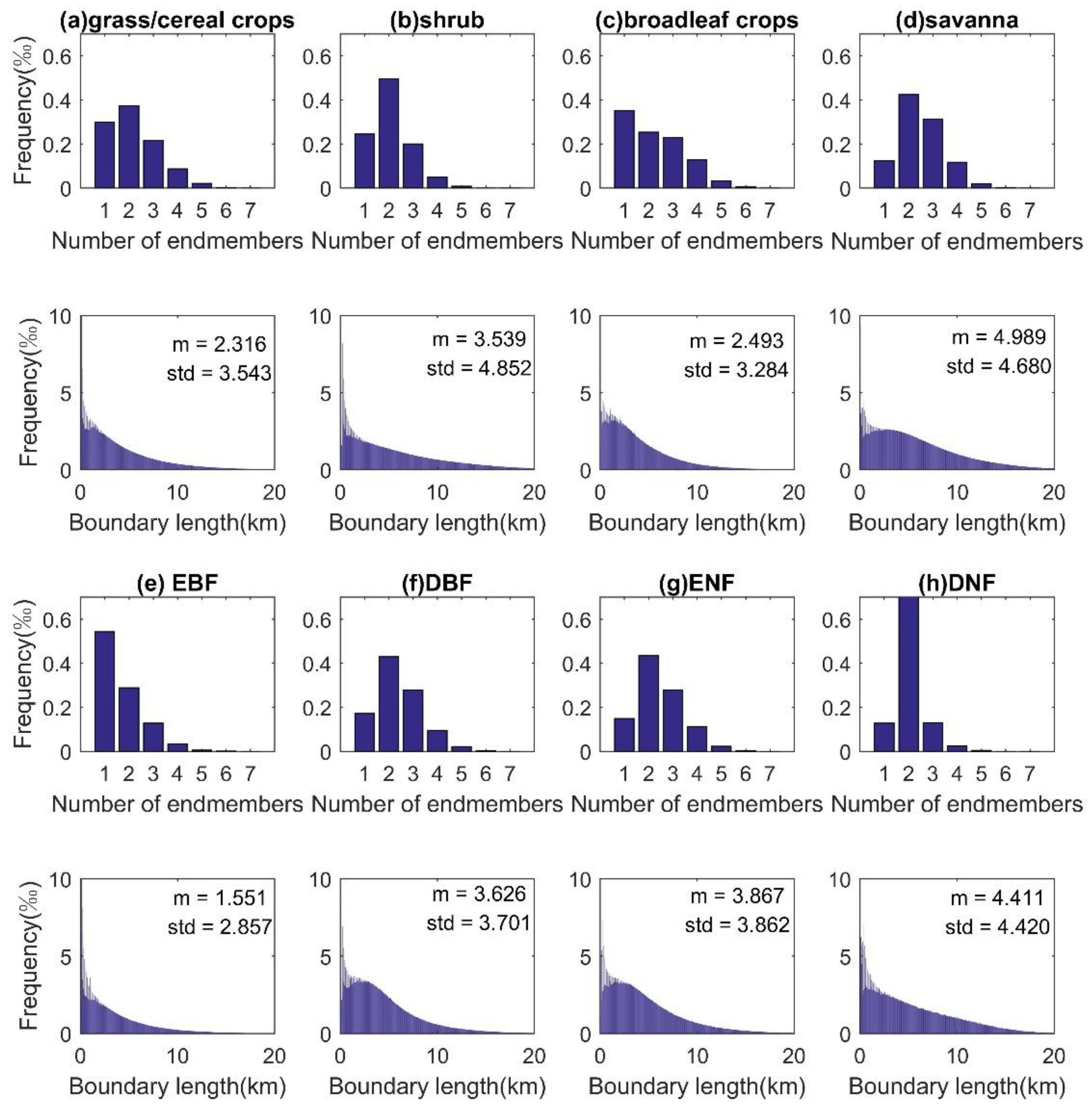
3.3. The Intra Heterogeneity of Typical Biomes

Moderate-resolution land cover products usually represent each pixel according to the dominant land cover. Parameter inversion algorithms using these land cover products inevitably overlook intra heterogeneity characteristics. For example, MODIS MCD12Q1 was adopted in LAI/FPAR products to characterize vegetation and soil properties in a pixel [41]. This characterization scheme was somehow unreasonable due to the intra land cover heterogeneity. A depiction of heterogeneity characteristics was needed to better parameterize the properties in typical biomes. The number of endmembers and the boundary length were analyzed for eight typical biomes (Figure 9): grasses/cereal crops, shrubs, broadleaf crops, savanna, evergreen broadleaf forest, deciduous broadleaf forest, evergreen needleleaf forest, and deciduous needleleaf forest.

Over 70% of the pixels in evergreen broadleaf forests are composed of one or two land cover types. Also, the average boundary length of evergreen broadleaf forests is the lowest (1551 m) of the eight biomes, which denotes the low heterogeneity of the biome at the 1-km scale. For deciduous needleleaf forests, 71.3% pixels are composed of two endmembers, while the boundary length is the second highest with m = 4411 m and std = 4420 m. Boreal forests with a grass understory make up the typical landscape pattern of the biome and should be the primary concern in the modeling and inversion of this biome. The deciduous broadleaf forest and evergreen needleleaf forest biomes have similar characteristics. Almost 15% of the pixels in these biomes are pure pixels, while most pixels have two or three endmembers (70.9%), and almost 12% of pixels are composed of four or five endmembers. The average boundary length and standard deviation are similar at approximately 3700 to 3800 m. These two forest types show moderate heterogeneity in forest biomes.

The grass/cereal crop and broadleaf crop biomes have high fractions of pure pixels at approximately 30.0% and 35.2%, respectively. The average boundary lengths of 2316 m and 2493 m are generally lower than those of other biomes. Grass and crop pixels exhibit low fragmentation, but mixtures with other land cover types are common. Human activities and the existence of the ecological transition zones may be the two primary reasons for the heterogeneity in grass and crop biomes. Savanna occupies the highest boundary length (m = 4989, std = 4680) of the eight biomes. Most of the pixels (73.8%) are mixed with two or three endmembers. Savanna pixels are more likely to be highly fragmented and include multiple cover types. Overall, the heterogeneity degree of biomes from high to low are as follows: savanna, deciduous needleleaf forest, evergreen needleleaf forest, deciduous broadleaf forest, shrub, broadleaf crops, grass/cereal crops, evergreen broadleaf forest.

3.4. Analysis of the Effective Boundary Length

Shadowing effects are closely associated with geometric conditions and boundary features (e.g., the orientation and canopy height differences in this paper). The effective influence of the boundary length on the radiative transfer process is analyzed based on a weighted boundary length by considering the orientation and canopy height difference separately. According to the formula of the effective boundary length and RTAF model simulations [25], the weights of various boundaries are normalized and given in

Table 2. Weights of boundary types. ’H’, ‘M’ and ‘L’ are symbols of canopy height ranks shown in Table 1. (‘-’ represents a west-east orientation; ’/’ represents a north-south orientation).

Boundary Type	${\mathit{w}}_{\mathit{i}}$	${\mathit{w}}_{\mathit{j}}$	Boundary Type	${\mathit{w}}_{\mathit{i}}$	${\mathit{w}}_{\mathit{j}}$
H-M	0	0.75	H/M	0.75	0.75
M-H	0	0.75	M/H	1	0.75
M-L	0	0.25	M/L	0.75	0.25
L-M	0	0.25	L/M	1	0.25
H-L	0	1	H/L	0.75	1
L-H	0	1	L/H	1	1

for the sun zenith angle, azimuth angle, and view zenith angle values of 45, 120, and 0 degrees, respectively.

Based on this information, the effective boundary lengths $B{L}_o^e$ and $B{L}_{hd}^e$ and the mean boundary lengths of the eight typical global biomes were calculated.

Table 3. Comparison of the mean boundary lengths of typical biomes for boundary length (BL), $B{L}_o^e$, and $B{L}_{hd}^e$.

Biome	Mean BL	Mean $\mathit{B}{\mathit{L}}_{\mathit{o}}^{\mathit{e}}$	Mean $\mathit{B}{\mathit{L}}_{\mathit{h}\mathit{d}}^{\mathit{e}}$	$\Delta \mathbf{m}1$	$\Delta \mathbf{m}2$
Grass/cereal crops	2316.1	1019.6	1410.4	55.98%	39.10%
Shrubs	3539.6	1545.9	2694.8	56.33%	23.87%
Broadleaf crops	2494	1093.7	1559.2	56.15%	37.48%
Savanna	4989.6	2194.8	3955.9	56.01%	20.72%
EBF	1551	679.7	1358.9	56.18%	12.39%
DBF	3626.9	1590.9	3097.6	56.14%	14.59%
ENF	3867.3	1696.9	3311.9	56.12%	14.36%
DNF	4411.5	1933	4323.5	56.18%	1.99%

presents the average total boundary length (BL), the effective boundary length considering orientation ($B{L}_o^e$, denoted as type 1), the effective boundary length considering boundary height differences ($B{L}_{hd}^e$, denoted as type 2), the percentage decreased between the mean boundary length and type 1 boundary length (∆m1), and the percentage decreased between the mean boundary length and type 2 boundary length (∆m2).

The effective boundary length reflects how much the boundary length impacts the radiative transfer process (∆m1 and ∆m2 reflect impacts from the orientation and canopy height difference, respectively). Table 3 shows that the impacts from the boundary orientation are significantly larger than those from the boundary canopy height difference (with the average ∆m1 and ∆m2 of 56.13% and 20.56%, respectively). In terms of boundary orientation, the eight biomes exhibit similar patterns, which suggests that the boundary orientations are similar (uniformly distributed) in different biomes. In other words, the bias associated with boundary orientation during the radiative transfer process is similar for all of the biomes. With respect to the canopy height differences, the ∆m2 values of the eight biomes exhibit evident differences. The mean effective boundary length of deciduous needleleaf forests only decreased by 1.99% compared to other biomes, which indicates that the differences in the boundary canopy height in this biome are notable and the associated influence on the radiative transfer model should not be neglected. Moreover, the effective boundary lengths of grass/cereal crops and broadleaf crops decreased by 39.10% and 37.48%, respectively, suggesting that the canopy height difference is not significant. In conclusion, the bias associated with canopy height differences is more notable in forests, especially deciduous needleleaf forests, than in other biomes.

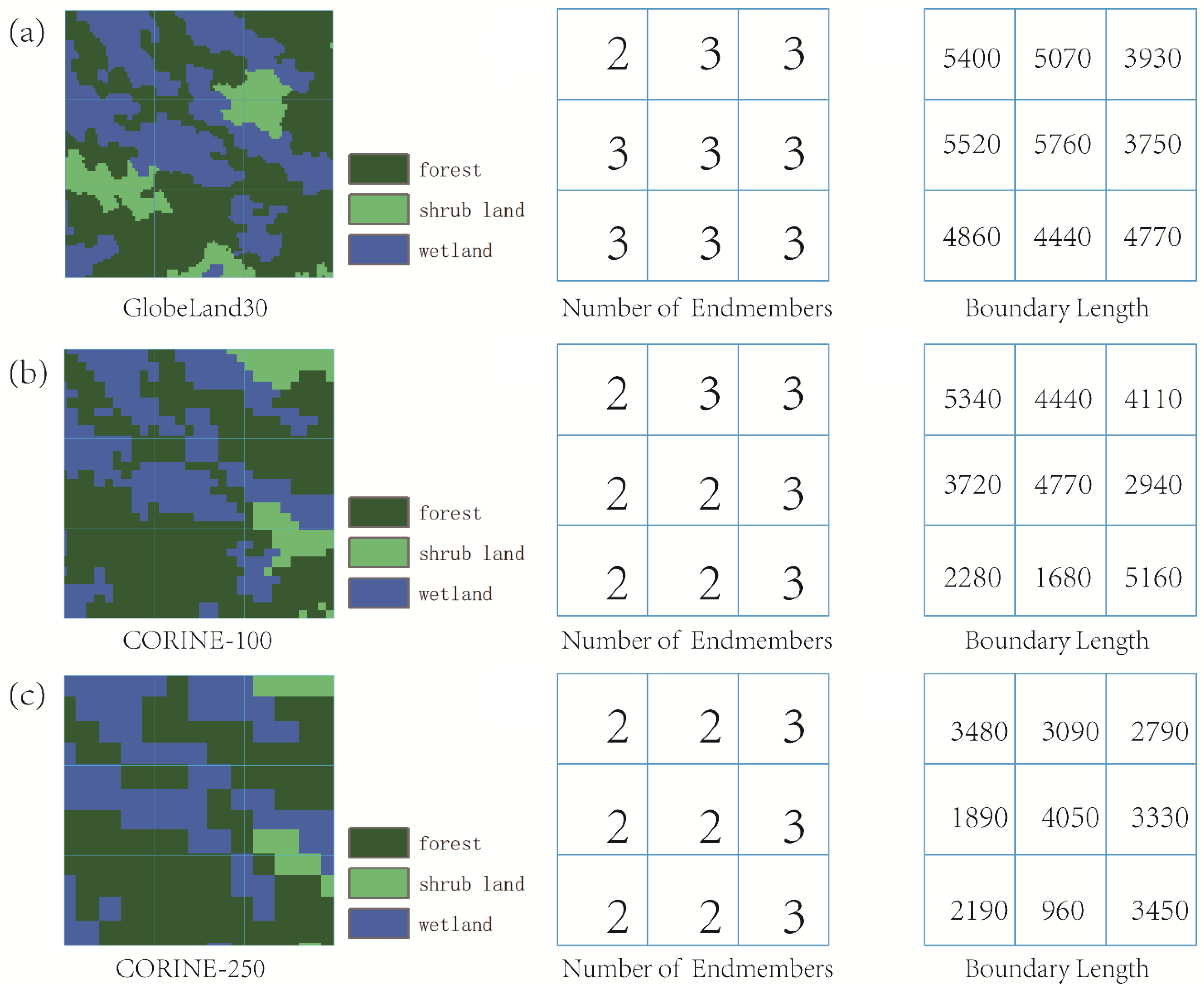
3.5. The Effects of Land Cover Data

The precision of extracted heterogeneity parameters is highly related to the accuracy as well as the resolution of input land cover data. A comparison of heterogeneity parameters extracted from GlobeLand30, CORINE-100, and CORINE-250 are displayed in Figure 10. The three land cover maps show good consistency with one another with respect to the number of endmembers, as well as a declining trend to the boundary length. There exists misclassification between shrubland and forest in Corine maps at the middle-left of the landscape. As a consequence, the number of endmembers of Globeland30 are a little larger than that of Corine at the same region. Misclassification and scale issues are the main sources of inconsistency. The misclassification of land cover types (e.g., wetland and shrubland in Figure 10) with same canopy height rank has little influence on the boundary length but would induce differences in the number of endmembers. The GlobeLand30 product adopted in this paper outperforms other global high-resolution land cover products in terms of accuracy. The land surface heterogeneity parameters calculated using GlobeLand30 is by far the most achievable way to obtain the global land surface heterogeneity in a quantitative manner. With the improvement of land cover product, more accurate knowledge of global land surface heterogeneity characteristics should be acquired.

4. Discussion

4.1. Strengths and Limitations of the Approach

The spatial heterogeneity within the moderate resolution pixel biases non-linear estimation processes of land surface variables from remote sensing data [1,23]. The parameterization of spatial heterogeneity is needed for the correct understanding of land surface estimation processes. The land cover heterogeneity characteristics can provide insights of the complexity of the variation in the land surface. Representing a scenario by composition and boundary information rather than dominant cover type provides a novel framework to account for land cover heterogeneity.

At a global scale, the selection and robustness of endmembers is a challenging problem. Zhan et al. [42] adopted three components: woody vegetation, herbaceous vegetation, and bare ground, to represent vegetation compositions at a 1-km resolution, thus offering sub-pixel information on vegetation monitoring. However, besides vegetation, other land cover types like water are also critical components of land surface, which is considered in our result. The aggregation of finer resolution information was applied to land use systems to account for landscape heterogeneity with scale of 5 arc-minutes [33] and showed superiority in land use and land cover change (LUCC) studies. In this paper, we explored the compositions of pixels at 1-km resolution and provided much more realistic information of land cover heterogeneity. The boundary information extracted in the paper mainly account for the abrupt transition of land covers with different vegetation canopy heights. The properties of the boundary can reflect the spatial configuration of land cover patches and account for the multi-scattering component of pixels.

Heterogenous regions have been identified from different perspectives. Considering the legend inconsistency of different land cover maps, areas of disagreement have been reported to occur in the northern transition zone of forest towards shrub cover (Russia and Canada) for global tree cover and the transition zone between savanna and desert (Northern Africa) for agricultural land [43]. A comparison of the current 1-km global land cover maps indicated that the transition zones of major ecosystems and areas of major human activities, such as boreal forests and tundra, savanna and major mountain ranges, appear as major areas of disagreement [9]. Our analysis results also indicated that these regions are of high heterogeneity, which may explain the disagreement between the 1-km resolution land cover maps and the provided detailed heterogeneity features (compositions and fragmentations) for these regions.

The uncertainty of heterogeneity characteristic estimation originates from land cover data. The accuracy of the land cover data directly determines the correctness of the extracted heterogeneity characteristic. The influence of misclassification is different for the calculation of different heterogeneity parameters. In general, the misclassification of land cover types with similar canopy heights has little influence on the boundary length or the effective boundary length (e.g., grassland and bare land), but would induce changes in the number of endmember results. The misclassification between land covers with different canopy heights introduces many uncertainties into the calculation of the effective boundary length. In the validation report of Globeland30, forest, cultivated land, and non-vegetated classes (water, artificial surfaces, and bare land) showed relatively higher accuracy (over 83% generally). Heterogeneity features involved with these classes promise to be more reliable. As the accuracy of grassland, shrubland, and wetland classes is relatively lower (about 73%), the robustness of heterogeneity features related to these classes needs to be improved. Therefore, the accuracy of the land cover product should be considered to meet the requirement of the application objective of the heterogeneity characteristic product.

The spatial resolution of land cover products also causes variations in the estimation of the heterogeneity characteristic. High-resolution land cover data can reveal more details of land surface difference, including the different land cover types and the difference inside each land cover type. The heterogeneity characteristic calculated based on land cover data with a higher resolution tends to result in more endmembers and a larger boundary length for each pixel, as shown in Figure 10. However, the relative fragmentation degree should be consistent under same scales. Different scales of the land cover data reveal the heterogeneity of the pixels in different stratifications. The selection of the land cover product depends on the application objective of the heterogeneity characteristic. Previous research showed that a pixel size with less than 100-m resolution is sufficient to capture the major part of the spatial variability in the vegetation cover at the landscape scale [1]. The resolution of 30 m used in this paper is capable of describing land cover heterogeneity in 1-km units. If the information of the variety inside each land cover types is needed in the heterogeneity characteristic, a resolution higher than 30 m should be applied, for example, 1-m resolution.

Due to the seasonal change of the land cover, the heterogeneity characteristic also has a seasonal variation. However, the high-resolution land cover products are generated usually on the baseline of one year. The change of the land cover change within a year cannot be well-presented from existing land cover products of 30-m resolution. For example, cultivated land would transfer to bare land after the harvest season, and the crop canopy height varies significantly with crop growth. Therefore, over the land cover types with obvious seasonal variation, the estimation of heterogeneity characteristic may have uncertainty caused by seasonal variation. Because the 30-m land cover products are generated in specific years, such as the GlobeLand30 generated in 2000 and 2010, when the estimation generated in a specific year is used in other years, the uncertainty caused by inter-annual variation of land cover products appears.

4.2. Potential Applications

Global heterogeneity characteristics could provide potential directions for future research involving radiative transfer modeling and parameter inversion algorithms. First, in the present inversion algorithms of satellite products, pixels are generally assumed to be covered with a single type. The analysis in this paper shows that the pixels mixed with water account for 21.3% of all mixed pixels, and the pixels mixed with artificial surfaces and permanent snow and ice account for 8.05% of all mixed pixels. These non-vegetation constituents can evidently affect pixel reflectance and cause obvious errors in vegetation parameter inversion. The heterogeneity parameters supply an indicator to separate the pixel mixture pattern and apply the corresponding inversion method to improve the inversion accuracy, which brings up the prospect of improving the total product accuracy. There are no radiative transfer models to simulate the scenes mosaicked by multiple vegetation types at present. The analysis in this paper shows that the pixels mixed with different vegetation types account for 64.0% of all pixels in global vegetated areas, which is the most common mixture pattern. The obvious height differences between different vegetation types over boundary areas will cause cross-radiation and shadowing effects, and these effects become non-negligible under some conditions. The land cover heterogeneity characteristics could contribute to the development of radiative transfer models to better simulate the bidirectional reflectance of globally, widely distributed mixed pixels.

The heterogeneity characteristics provide detailed information of pixels beyond just identifying these regions for the application of landscape typology and land use systems. The sub-pixel composition helps to determine where the disagreements come from and to elucidate precise land cover variation within a spatial unit; the boundary information reflects the landscape structure and fragmentation degree, which are known to relate to ecosystem services [44] and landscape aesthetics [45], and could also be utilized the for assessment of landscapes. A recent study suggested that heterogeneous landscapes may need to be explicitly represented as separate classes in future products [10]; therefore, the mixture pattern displayed in our results could be valuable to relevant developers. Moreover, it can serve as a basis of sampling or selecting validation sites with considerations of heterogeneity features [46,47,48,49].

5. Conclusions

At moderate spatial resolutions, the heterogeneity of pixels is a key problem that affects the precise simulation of the radiative transfer processes and accurate inversion of land surface parameters. This paper presents a parameterization scheme to describe pixel heterogeneity quantitatively based on compositions and boundary information from high-resolution land cover data. This scheme provides an approach to evaluate the heterogeneity characteristics of global mixed pixels and analyze the influence of land cover heterogeneity on mixed pixel modeling. The following conclusions were drawn from this study:

(1)

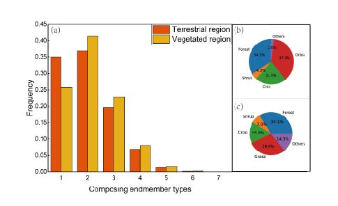
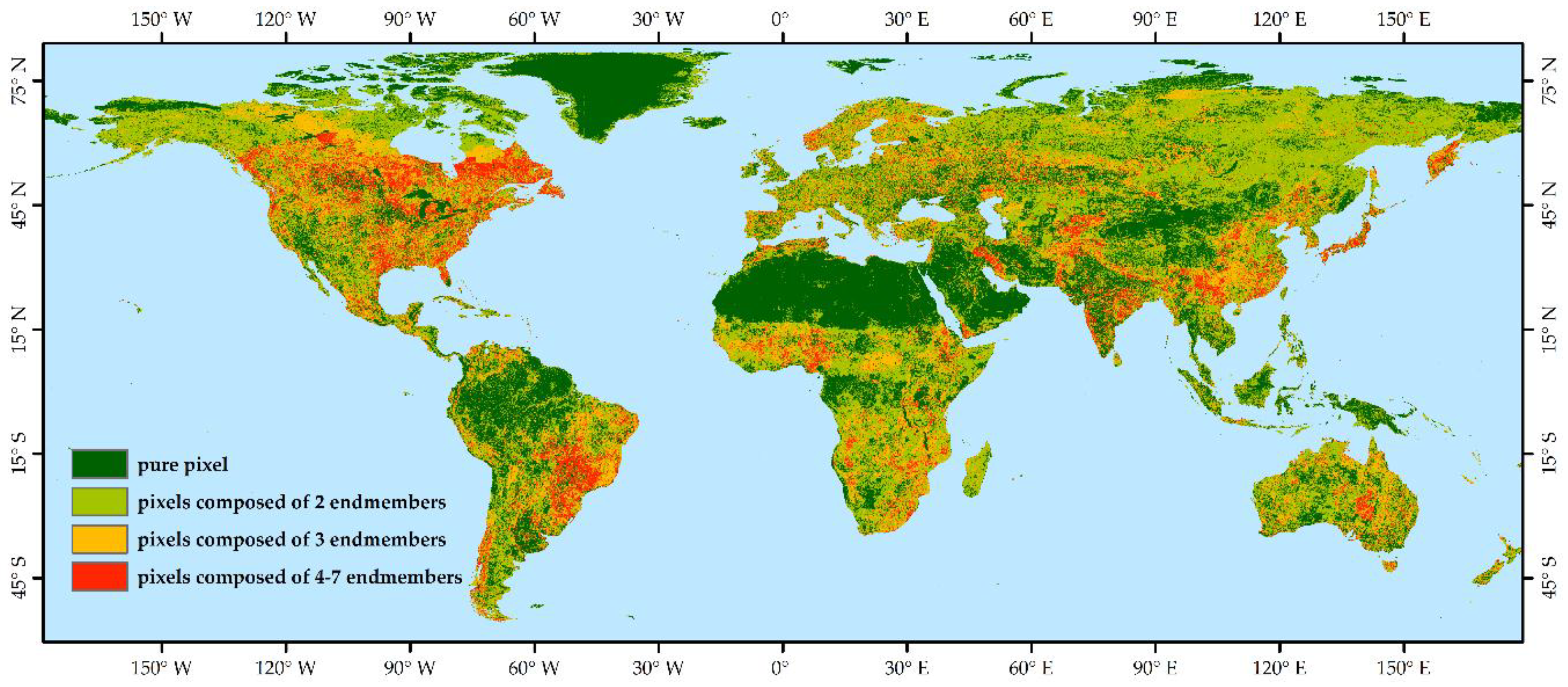
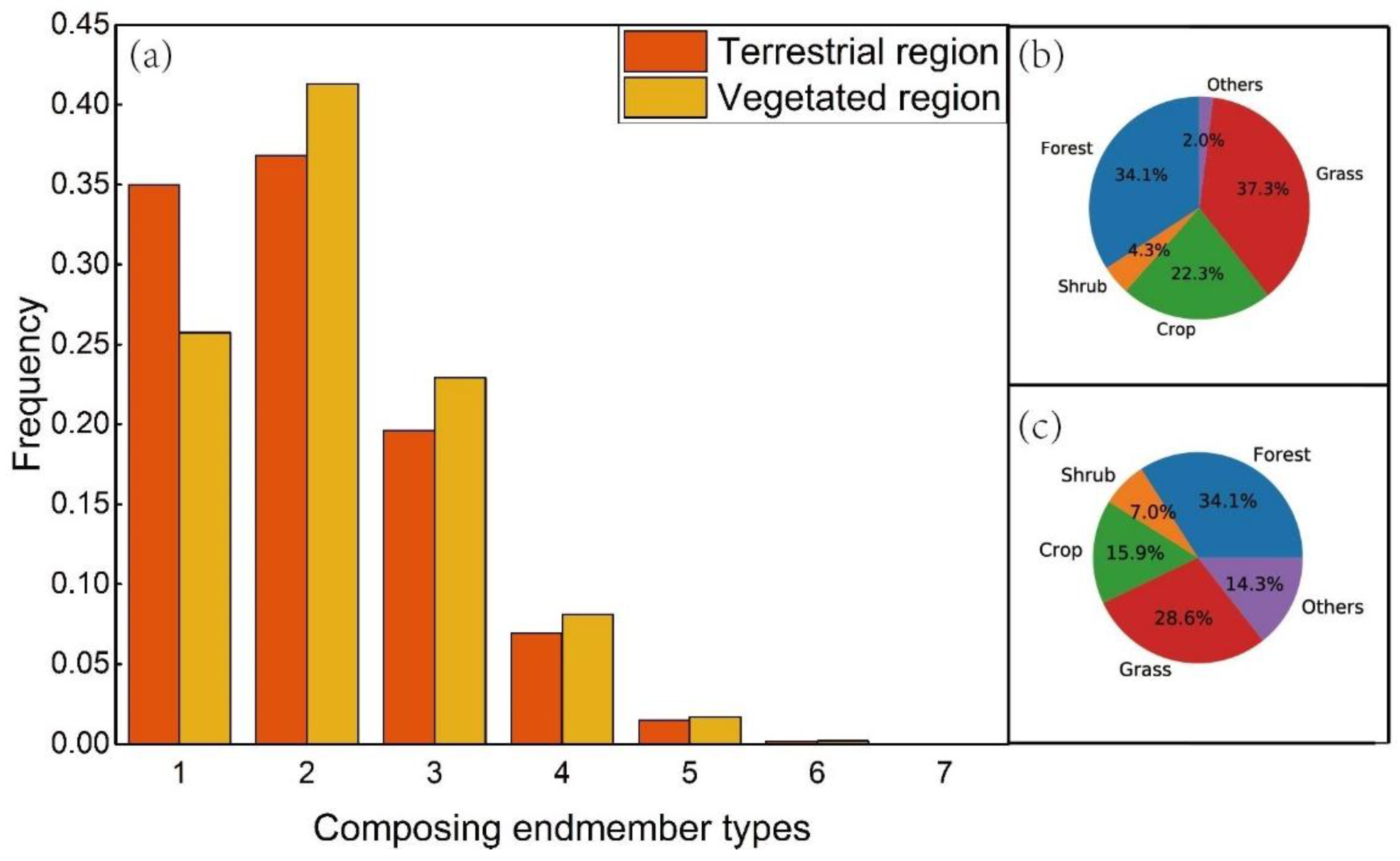
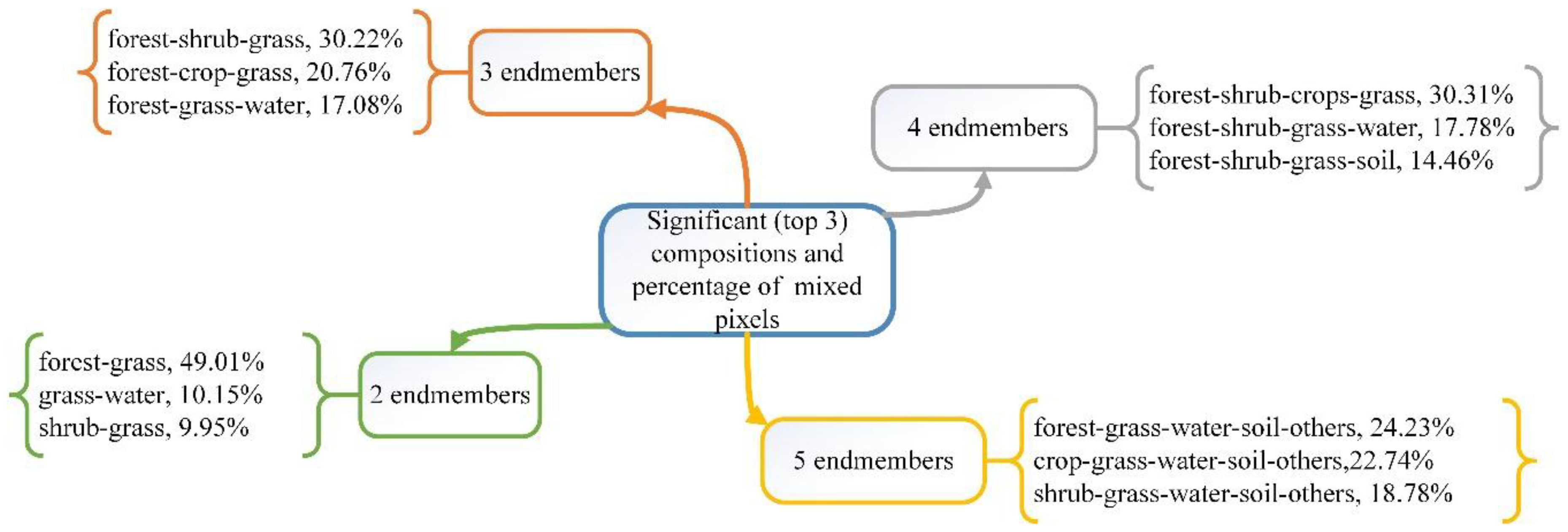
At the 1-km scale, heterogeneity caused by the mixture of different land cover types exists globally. Only 35% of pixels over the land surface of Earth are covered by a single land cover type, namely, pure pixels, and only 25.8% of them are located in vegetated areas. The composition analysis yielded two main findings. First, most pixels are characterized by mixtures of different vegetation types, accounting for 64.0% of all pixels in global vegetated areas. Large amounts of mixed pixels are composed of endmembers with different canopy heights, which are more commonly existed in ecological transition zones. Second, mixed pixels with water are more common than mixed pixels with any other non-vegetation type, accounting for 21.3% of all mixed pixels.

(2)

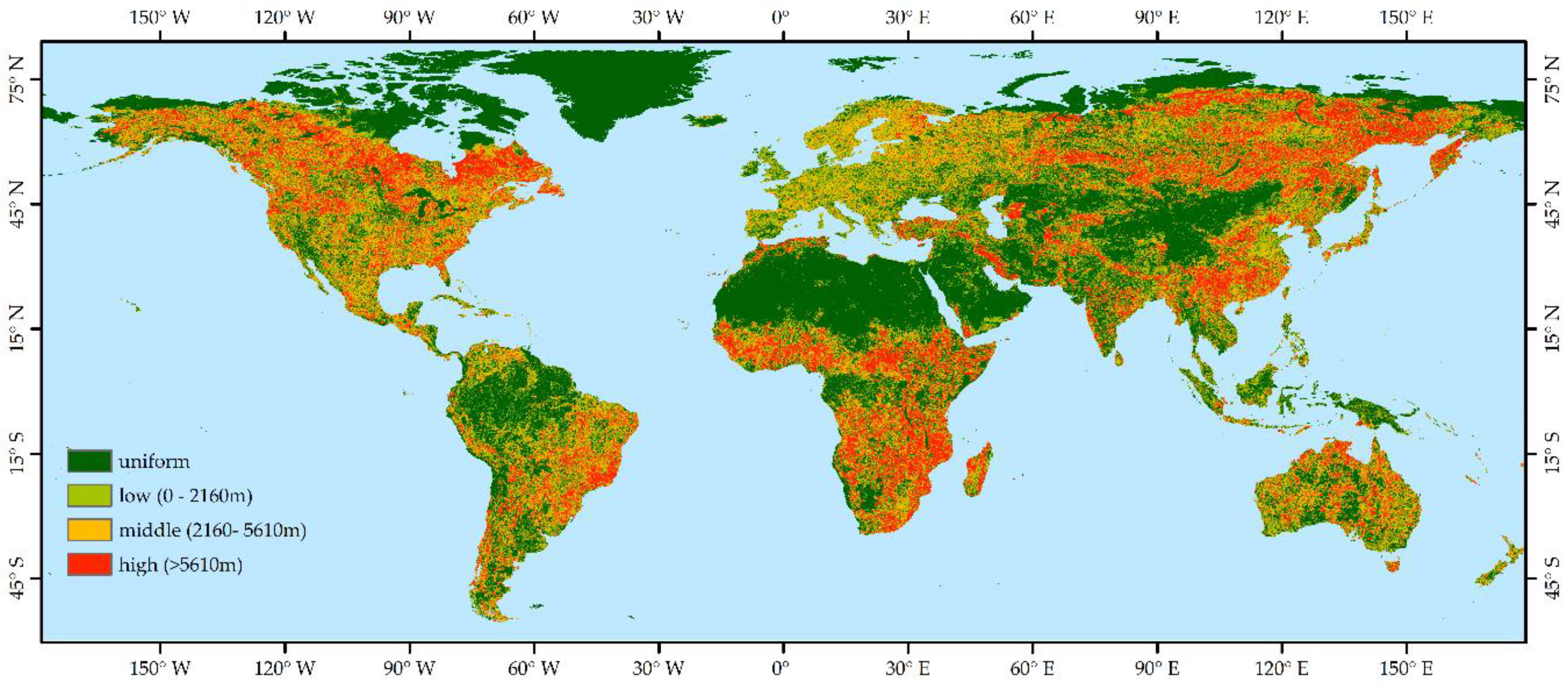
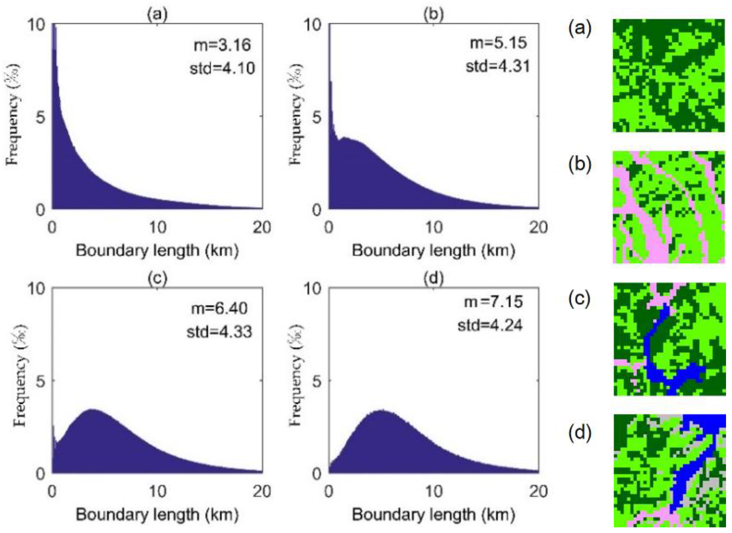
Mixed pixels with more endmembers are generally more fragmented, though pixels with two endmembers could be extremely fragmented. Eight typical biomes exhibited obvious but different intra heterogeneity features at global extents. The land surface in biomes are far from uniform, as is assumed in many product algorithms. The heterogeneity degree of biomes from high to low are: savanna, deciduous needleleaf forest, evergreen needleleaf forest, deciduous broadleaf forest, shrub, broadleaf crops, grass/cereal crops, evergreen broadleaf forest. The biases associated with boundary orientation during radiative processes are similar, while biases caused by canopy height differences are not the same in all biomes. Deciduous needleleaf forest areas are significantly affected by canopy height differences, while grass/cereal crops and broadleaf crops are less affected.

This paper analyzed global heterogeneity characteristics at a 1-km scale with the aim of contributing to the establishment of heterogenous models and improving the inversion accuracy of satellite products at a moderate resolution. The detailed impacts of land cover heterogeneity characteristics on parameter inversion and the utilization of the features in modeling warrant further exploration.

References

1. Garrigues, S.; Allard, D.; Baret, F.; Weiss, M. Influence of landscape spatial heterogeneity on the non-linear estimation of leaf area index from moderate spatial resolution remote sensing data. Remote Sens. Environ. 2006, 105, 286–298. [Google Scholar] [CrossRef]
2. Tian, Y.; Woodcock, C.E.; Wang, Y.; Privette, J.L.; Shabanov, N.V.; Zhou, L.; Zhang, Y.; Buermann, W.; Dong, J.; Veikkanen, B. Multiscale analysis and validation of the modis lai product: I. Uncertainty assessment. Remote Sens. Environ. 2002, 83, 414–430. [Google Scholar] [CrossRef]
3. Myneni, R.; Hoffman, S.; Knyazikhin, Y.; Privette, J.; Glassy, J.; Tian, Y.; Wang, Y.; Song, X.; Zhang, Y.; Smith, G. Global products of vegetation leaf area and fraction absorbed par from year one of modis data. Remote Sens. Environ. 2002, 83, 214–231. [Google Scholar] [CrossRef]
4. Friedl, M.A.; McIver, D.K.; Hodges, J.C.; Zhang, X.; Muchoney, D.; Strahler, A.H.; Woodcock, C.E.; Gopal, S.; Schneider, A.; Cooper, A. Global land cover mapping from modis: Algorithms and early results. Remote Sens. Environ. 2002, 83, 287–302. [Google Scholar] [CrossRef]
5. Jacob, F.; Weiss, M. Mapping biophysical variables from solar and thermal infrared remote sensing: Focus on agricultural landscapes with spatial heterogeneity. IEEE Geosci. Remote Sens. Lett. 2014, 11, 1844–1848. [Google Scholar] [CrossRef]
6. Yin, G.; Li, J.; Liu, Q.; Li, L.; Zeng, Y.; Xu, B.; Yang, L.; Zhao, J. Improving leaf area index retrieval over heterogeneous surface by integrating textural and contextual information: A case study in the heihe river basin. IEEE Geosci. Remote Sens. Lett. 2015, 12, 359–363. [Google Scholar]
7. Friedl, M.A.; Sulla-Menashe, D.; Tan, B.; Schneider, A.; Ramankutty, N.; Sibley, A.; Huang, X. Modis collection 5 global land cover: Algorithm refinements and characterization of new datasets. Remote Sens. Environ. 2010, 114, 168–182. [Google Scholar] [CrossRef]
8. Zomer, R.J.; Trabucco, A.; Coe, R.; Place, F. Trees on Farm: Analysis of Global Extent and Geographical Patterns of Agroforestry; ICRAF Working Paper; World Agroforestry Centre: Nairobi, Kenya, 2009. [Google Scholar]
9. Herold, M.; Mayaux, P.; Woodcock, C.E.; Baccini, A.; Schmullius, C. Some challenges in global land cover mapping: An assessment of agreement and accuracy in existing 1 km datasets. Remote Sens. Environ. 2008, 112, 2538–2556. [Google Scholar] [CrossRef]
10. Verburg, P.H.; Neumann, K.; Nol, L. Challenges in using land use and land cover data for global change studies. Glob. Chang. Biol. 2011, 17, 974–989. [Google Scholar] [CrossRef] [Green Version]
11. Chen, J.M. Spatial scaling of a remotely sensed surface parameter by contexture. Remote Sens. Environ. 1999, 69, 30–42. [Google Scholar] [CrossRef]
12. Tian, Y.; Wang, Y.; Zhang, Y.; Knyazikhin, Y.; Bogaert, J.; Myneni, R.B. Radiative transfer based scaling of lai retrievals from reflectance data of different resolutions. Remote Sens. Environ. 2003, 84, 143–159. [Google Scholar] [CrossRef]
13. Fang, H.; Li, W.; Myneni, R. The impact of potential land cover misclassification on modis leaf area index (lai) estimation: A statistical perspective. Remote Sens. 2013, 5, 830–844. [Google Scholar] [CrossRef]
14. Gilabert, M.A.; Garciaharo, F.J.; Melia, J. A mixture modeling approach to estimate vegetation parameters for heterogeneous canopies in remote sensing. Remote Sens. Environ. 2000, 72, 328–345. [Google Scholar] [CrossRef]
15. Liang, S. Numerical experiments on the spatial scaling of land surface albedo and leaf area index. Remote Sens. Rev. 2000, 19, 225–242. [Google Scholar] [CrossRef]
16. Kobayashi, H.; Suzuki, R.; Nagai, S.; Nakai, T.; Kim, Y. Spatial scale and landscape heterogeneity effects on fapar in an open-canopy black spruce forest in interior alaska. IEEE Geosci. Remote Sens. Lett. 2014, 11, 564–568. [Google Scholar] [CrossRef]
17. Kobayashi, H.; Iwabuchi, H. A coupled 1-d atmosphere and 3-d canopy radiative transfer model for canopy reflectance, light environment, and photosynthesis simulation in a heterogeneous landscape. Remote Sens. Environ. 2008, 112, 173–185. [Google Scholar] [CrossRef]
18. Huang, H.; Qin, W.; Liu, Q. Rapid: A radiosity applicable to porous individual objects for directional reflectance over complex vegetated scenes. Remote Sens. Environ. 2013, 132, 221–237. [Google Scholar] [CrossRef]
19. Qin, W.; Gerstl, S.A. 3-d scene modeling of semidesert vegetation cover and its radiation regime. Remote Sens. Environ. 2000, 74, 145–162. [Google Scholar] [CrossRef]
20. Widlowski, J.-L.; Pinty, B.; Lavergne, T.; Verstraete, M.M.; Gobron, N. Horizontal radiation transport in 3-D forest canopies at multiple spatial resolutions: Simulated impact on canopy absorption. Remote Sens. Environ. 2006, 103, 379–397. [Google Scholar] [CrossRef]
21. Haralick, R.M.; Shanmugam, K.S. Combined spectral and spatial processing of erts imagery data. Remote Sens. Environ. 1974, 3, 3–13. [Google Scholar] [CrossRef]
22. De Cola, L. Fractal analysis of a classified Landsat scene. Photogramm. Eng. Remote Sens. 1989, 55, 601–610. [Google Scholar]
23. Garrigues, S.; Allard, D.; Baret, F.; Weiss, M. Quantifying spatial heterogeneity at the landscape scale using variogram models. Remote Sens. Environ. 2006, 103, 81–96. [Google Scholar] [CrossRef]
24. Hintz, M.; Lennartz-Sassinek, S.; Liu, S.; Shao, Y. Quantification of land-surface heterogeneity via entropy spectrum method. J. Geophys. Res. 2014, 119, 8764–8777. [Google Scholar] [CrossRef] [Green Version]
25. Zeng, Y.; Li, J.; Liu, Q.; Huete, A.R.; Yin, G.; Xu, B.; Fan, W.; Zhao, J.; Yan, K.; Mu, X. A radiative transfer model for heterogeneous agro-forestry scenarios. IEEE Trans. Geosci. Remote Sens. 2016, 54, 4613–4628. [Google Scholar] [CrossRef]
26. Li, X.; Strahler, A.H. Geometric-optical bidirectional reflectance modeling of the discrete crown vegetation canopy: Effect of crown shape and mutual shadowing. IEEE Trans. Geosci. Remote Sens. 1992, 30, 276–292. [Google Scholar] [CrossRef]
27. Van der Zanden, E.H.; Levers, C.; Verburg, P.H.; Kuemmerle, T. Representing composition, spatial structure and management intensity of european agricultural landscapes: A new typology. Landsc. Urban Plan. 2016, 150, 36–49. [Google Scholar] [CrossRef]
28. Van Asselen, S.; Verburg, P.H. A land system representation for global assessments and land-use modeling. Glob. Chang. Biol. 2012, 18, 3125–3148. [Google Scholar] [CrossRef] [PubMed] [Green Version]
29. Elmore, A.J.; Mustard, J.F.; Manning, S.J.; Lobell, D.B. Quantifying vegetation change in semiarid environments: Precision and accuracy of spectral mixture analysis and the normalized difference vegetation index. Remote Sens. Environ. 2000, 73, 87–102. [Google Scholar] [CrossRef]
30. Adams, J.B.; Smith, M.O.; Johnson, P.E. Spectral mixture modeling: A new analysis of rock and soil types at the Viking Lander 1 site. J. Geophys. Res. Solid Earth 1986, 91, 8098–8112. [Google Scholar] [CrossRef]
31. Mustard, J.F.; Pieters, C.M. Abundance and distribution of ultramafic microbreccia in moses rock dike: Quantitative application of mapping spectroscopy. J. Geophys. Res. Solid Earth 1987, 92, 10376–10390. [Google Scholar] [CrossRef]
32. Mayaux, P.; Lambin, E.F. Tropical forest area measured from global land-cover classifications: Inverse calibration models based on spatial textures. Remote Sens. Environ. 1997, 59, 29–43. [Google Scholar] [CrossRef]
33. Letourneau, A.; Verburg, P.H.; Stehfest, E. A land-use systems approach to represent land-use dynamics at continental and global scales. Environ. Model. Softw. 2012, 33, 61–79. [Google Scholar] [CrossRef]
34. Li, X.; Strahler, A.H. Geometric-optical modeling of a conifer forest canopy. IEEE Trans. Geosci. Remote Sens. 1985, GE-23, 705–721. [Google Scholar] [CrossRef]
35. Ray, T.W.; Murray, B.C. Nonlinear spectral mixing in desert vegetation. Remote Sens. Environ. 1996, 55, 59–64. [Google Scholar] [CrossRef]
36. Belward, A.S. Glc2000: A new approach to global land cover mapping from earth observation data. Int. J. Remote Sens. 2007, 26, 1959–1977. [Google Scholar]
37. Chen, J.; Chen, J.; Liao, A.; Cao, X.; Chen, L.; Chen, X.; He, C.; Han, G.; Peng, S.; Lu, M. Global land cover mapping at 30m resolution: A pok-based operational approach. ISPRS J. Photogramm. Remote Sens. 2015, 103, 7–27. [Google Scholar] [CrossRef]
38. Adams, M.L.; Philpot, W.D.; Norvell, W.A. Yellowness index: An application of spectral second derivatives to estimate chlorosis of leaves in stressed vegetation. Int. J. Remote Sens. 1999, 20, 3663–3675. [Google Scholar] [CrossRef]
39. Smith, M.O.; Ustin, S.L.; Adams, J.B.; Gillespie, A.R. Vegetation in deserts: I. A regional measure of abundance from multispectral images. Remote Sens. Environ. 1990, 31, 1–26. [Google Scholar] [CrossRef]
40. Sohn, Y.; Mccoy, R.M. Mapping desert shrub rangeland using spectral unmixing and modeling spectral mixtures with TM data. Photogramm. Eng. Remote Sens. 1997, 63, 707–716. [Google Scholar]
41. Knyazikhin, Y.; Martonchik, J.; Myneni, R.; Diner, D.; Running, S. Synergistic algorithm for estimating vegetation canopy leaf area index and fraction of absorbed photosynthetically active radiation from modis and misr data. J. Geophys. Res. Atmos. 1998, 103, 32257–32275. [Google Scholar] [CrossRef]
42. Zhan, X.; De Fries, R.; Hansen, M.; Townshend, J.; Miceli, C.D.; Sohlberg, R.; Huang, C. MODIS Enhanced Land Cover and Land Cover Change Product, Algorithm Theoretical Basis Documents (ATBD), Version 20. 1999. Available online: https://lpdaac.usgs.gov/sites/default/files/public/product_documentation/mod44b_atbd.pdf (accessed on 1 March 2018).
43. Fritz, S.; See, L. Identifying and quantifying uncertainty and spatial disagreement in the comparison of global land cover for different applications. Glob. Chang. Biol. 2008, 14, 1057–1075. [Google Scholar] [CrossRef]
44. Schulp, C.J.E.; Lautenbach, S.; Verburg, P.H. Quantifying and mapping ecosystem services: Demand and supply of pollination in the European Union. Ecol. Indic. 2014, 36, 131–141. [Google Scholar] [CrossRef]
45. Gobster, P.H.; Nassauer, J.I.; Daniel, T.C.; Fry, G. The shared landscape: What does aesthetics have to do with ecology? Landsc. Ecol. 2007, 22, 959–972. [Google Scholar] [CrossRef]
46. Baret, F.; Weiss, M.; Allard, D.; Garrigues, S.; Leroy, M.; Jeanjean, H.; Fernandes, R.; Myneni, R.; Privette, J.; Morisette, J. VALERI: A network of sites and a methodology for the validation of medium spatial resolution land satellite products. Remote Sens. Environ. 2005, 76, 36–39. [Google Scholar]
47. Morisette, J.T.; Privette, J.L.; Justice, C.O. A framework for the validation of modis land products. Remote Sens. Environ. 2002, 83, 77–96. [Google Scholar] [CrossRef]
48. Zeng, Y.; Li, J.; Liu, Q.; Li, L.; Xu, B.; Yin, G.; Peng, J. A sampling strategy for remotely sensed LAI product validation over heterogeneous land surfaces. IEEE J. Sel. Top. Appl. Earth Obs. Remote Sens. 2014, 7, 3128–3142. [Google Scholar] [CrossRef]
49. Zeng, Y.; Li, J.; Liu, Q.; Qu, Y.; Huete, A.R.; Xu, B.; Yin, G.; Zhao, J. An optimal sampling design for observing and validating long-term leaf area index with temporal variations in spatial heterogeneities. Remote Sens. 2015, 7, 1300–1319. [Google Scholar] [CrossRef]
Figure 1. Global distribution of biome types in 2010 based on the moderate resolution imaging spectroradiometer (MODIS) Leaf Area Index (LAI)/Fraction of Absorbed Photosynthetically Active Radiation (FPAR) (Type 3) classification system.
Remotesensing 10 00856 g001
Figure 2. Thirty-meter resolution land cover maps of three 1-km resolution pixels with different degrees of fragmentation.
Remotesensing 10 00856 g002
Figure 3. Flow chart describing the extraction procedures of land cover heterogeneity.
Remotesensing 10 00856 g003
Figure 4. Global distribution of the number of endmembers at a 1-km resolution.
Remotesensing 10 00856 g004
Figure 5. Frequency histogram of endmember count for 1-km resolution pixels; terrestrial region refers to land regions excluding Antarctica on the Earth. The pie chart (b,c) demonstrates the fraction of endmember classes of pure pixels over vegetation regions and the overall proportions of endmember classes over terrestrial regions.
Remotesensing 10 00856 g005
Figure 6. Significant combinations of 1-km resolution mixed pixels with two to five end members.
Remotesensing 10 00856 g006
Figure 7. Global boundary length map at 1-km resolution. The boundary lengths were classified into four categories by quantile. The longest 25% were taken as high fragmented; the boundary lengths between the top 50 and 25% were considered to be middle fragmented.
Remotesensing 10 00856 g007
Figure 8. Frequency distribution of the boundary length for different endmember types ((ad) represent two, three, four, and five endmembers, respectively) and the corresponding land cover images for a boundary length of 20,000 m. ‘m’ and ‘std’ stand for mean and standard deviation of the boundary length, respectively.
Remotesensing 10 00856 g008
Figure 9. Frequency distributions of different endmember numbers and boundary lengths for different biomes (EBF, DBF, ENF, and DNF stand for evergreen broadleaf forest, deciduous broadleaf forest, evergreen needleleaf forest, and deciduous needleleaf forest, respectively).
Remotesensing 10 00856 g009
Figure 10. Comparison between input land cover data with different resolutions.
Remotesensing 10 00856 g010