Article

Quantitative Assessment of Digital Image Correlation Methods to Detect and Monitor Surface Displacements of Large Slope Instabilities

by
Valentin Tertius Bickel
1,2,
Andrea Manconi
1,* and
Florian Amann
1,3
1
Engineering Geology, Swiss Federal Institute of Technology Zurich, 8092 Zurich, Switzerland
2
Department Planets and Comets, Max Planck Institute for Solar System Research, 37077 Goettingen, Germany
3
Lehrstuhl für Ingenieurgeologie und Hydrogeologie, RWTH Aachen University, 52064 Aachen, Germany
*
Author to whom correspondence should be addressed.
Submission received: 1 May 2018 / Revised: 15 May 2018 / Accepted: 30 May 2018 / Published: 1 June 2018
(This article belongs to the Special Issue Landslide Hazard and Risk Assessment)

Abstract

:
We evaluate the capability of three different digital image correlation (DIC) algorithms to measure long-term surface displacement caused by a large slope instability in the Swiss Alps. DIC was applied to high-resolution optical imagery taken by airborne sensors, and the accuracy of the displacements assessed against global navigation satellite system measurements. A dynamic radiometric correction of the input images prior to DIC application was shown to enhance both the correlation success and accuracy. Moreover, a newly developed spatial filter considering the displacement direction and magnitude proved to be an effective tool to enhance DIC performance and accuracy. Our results show that all algorithms are capable of quantifying slope instability displacements, with average errors ranging from 8 to 12% of the observed maximum displacement, depending on the DIC processing parameters, and the pre- and postprocessing of the in- and output. Among the tested approaches, the results based on a fast Fourier transform correlation approach provide a considerably better spatial coverage of the displacement field of the slope instability. The findings of this study are relevant for slope instability detection and monitoring via DIC, especially in the context of an ever-increasing availability of high-resolution air- and spaceborne imagery.

Graphical Abstract

1. Introduction

Catastrophic landslides are responsible for about 1000 fatalities per year [1,2], while causing total financial costs for direct infrastructure restoration and remedial, as well as indirect economic productivity losses in the order of billions of US dollars [3,4]. In general, slope instabilities are geomorphological processes that involve the movement of soil or rock driven by gravity [3]. Predisposing factors for slope instabilities include e.g., the topography of the slope, the type of the rock or soil and its structure and lateral constraints [5]. Slope failures are finally triggered by heavy rainfall events, snowmelt, earthquakes, or human activity [6]. Prior to failure, the deformation of a slope’s surface is one of the main parameters that allow for describing and observing the temporal evolution of slope instabilities, to understand their behavior, and to predict their potential failure [5,7,8]. The slow and continuous displacement of slopes over long periods of time can also be utilized to detect previously unknown instabilities and assess their hazard potential.
In this scenario, ground-based monitoring instruments may provide important information on displacements; however, these methods are often impractical for this purpose. For example, access to failure-prone slopes can be hazardous, thus, the installation of in situ monitoring equipment can be dangerous [9]. Moreover, regional scale analyses or even at the scale of a single slope implies high costs. The application of remote sensing techniques enables also the extraction of information about the evolution of the slope instability. Within the last decade, air- and spaceborne remote sensing methods using active sensors, such as differential synthetic aperture radar (SAR) interferometry (DInSAR) [5,10,11], or methods using input from passive sensors, such as digital image correlation (DIC) [12,13,14,15,16], have been established to detect and monitor surface displacements at regional scales.
DIC, also known as feature-tracking or subpixel offset [15], is an image processing technique that identifies and quantifies ground displacement occurring orthogonal to the line-of-sight (LOS) of the camera [17]. Amongst others, DIC has been applied to monitor the glacier velocities [18,19], the ground displacement caused by earthquakes or tectonic activity [17,20], and the deformations at volcanoes [21]. A selection of application examples for DIC is listed in Table 1. While DIC can be applied on various types of input data from different platforms, its primary potential for slope instability detection and monitoring lies in the utilization of high-resolution optical imagery, acquired by satellites [22] and manned or unmanned aerial vehicles (UAVs) [23]. The exploitation of such data enables a detailed investigation and observation of slope instabilities on a local and on a regional scale, in any terrain. DIC analysis can provide key information on the spatial and temporal evolution of surface displacements at large slope instabilities; however, its potential and accuracy has not been thoroughly evaluated yet.
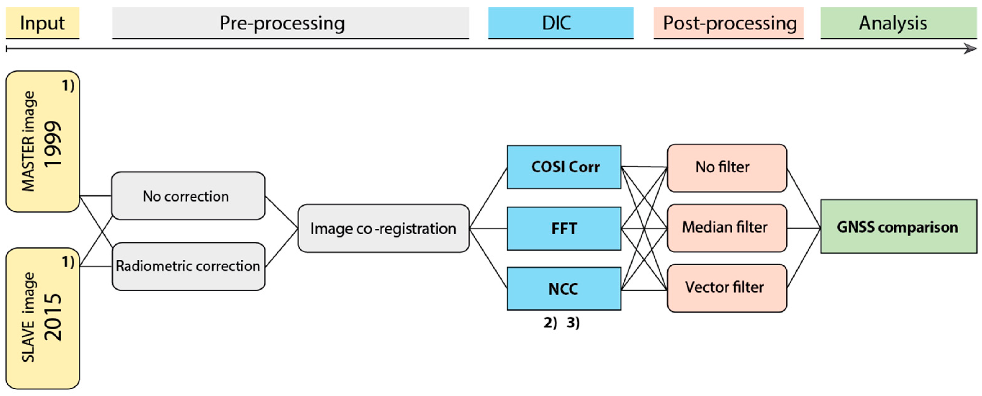
In order to provide new insights in this context, here, we investigate the qualitative and quantitative ability of three commonly used DIC algorithms to measure the deformation of a deep-seated gravitational slope deformation (DSGSD) located in the Swiss Alps. Two high-resolution optical images taken from airborne sensors optical images spanning 16 years were used as input for the DIC analyses. The results were compared to 23 points across the DSGSD, monitored via global navigation satellite system (GNSS) in the same time period.
In the following sections, we introduce the study site, followed by a short description of the DIC approach. Subsequently, we present the data used and the workflow. Next, we describe the derived results and discuss their implications. In the appendices, we provide detailed information on technical aspects of this study.

2. Study Site Introduction

The study area is a major deep seated gravitational slope deformation (DSGSD) at the Cuolm da Vi (CdV) in the Canton Graubünden, Switzerland (Figure 1), situated on a south-facing mountain slope north of the town Sedrun in the Central Alps, on the southern boundary of the Aar Massif. CdV has an estimated unstable volume of roughly 150 million cubic meters [37,38,39]. The toe of the DSGSD towards the S-SE is characterized by active and rapid gullying processes, such as erosion and shallow slope instabilities (Figure 1b). The ongoing SW-wards deformation is expressed on the surface by typical landslide related morphological structures, such as local instabilities (Figure 1a), graben structures, scarps, and deep tension cracks (Figure 1c), which indicate a gravitational displacement along inherited tectonic structures [37]. According to [37] the average displacement rates across the area are around 20 cm per year.

3. Materials and Methods

DIC is an image processing technique aimed at identifying and quantifying displacements using multitemporal digital imagery. Thus, DIC applies algorithms that first geometrically align two or more images of the same area acquired at different times (in the following, master refers to the older image, while slave to the more recent one), by relying on control points [41]. Subsequently, DIC evaluates internal misalignment using a moving template window, while measuring displacements that occurred in the time span between master and slave acquisition. DIC approaches are sensitive to displacements along the two spatial directions orthogonal to the camera line of sight or parallel to the camera view plane (CVP). Out-of-CVP deformation cannot be measured with DIC, being primarily the vertical component in case of nadir looking air- or spaceborne sensors.
There are various algorithms that apply the DIC principle, while the most popular codes operate either in the spatial or in the frequency domain, implementing either normalized cross correlation (NCC) or fast Fourier transformation (FFT) approaches, respectively [22]. In this work, three implementations of different algorithms were selected, one utilizing a NCC, another using a FFT approach and one established code that is being distributed by the Caltech Tectonics Observatory, called COSI Corr, operating in the frequency domain as well [22]. Details about the assessed codes can be reviewed in Appendix A.1, Appendix A.2, Appendix A.3 of the Appendix A.

3.1. Dataset

Orthorectified aerial photographs, as well as GNSS data from the area of interest (AoI), have been utilized for this study. The aerial images were acquired and processed in the years 1999 and 2015 under snow- and cloud-free conditions. The 1999 acquisition has been taken by a Leica ADS80 mounted on a manned aircraft, while the 2015 image was captured with an “ebee” fixed-wing drone produced by the company Sensefly [42], equipped with a Canon S 110 RGB. Both images were orthorectified using the swissALTI3D by swisstopo, processed to 8 bit single band images, and have a final GSD (ground sampling distance) of 0.25 m/pixel. The 2015 acquisition has been downsampled to fit the GSD of the 1999 acquisition. The selected images allow a comparison over a temporal baseline of 16 years. Due to the spatial extent of the acquisition of the available 1999 master image, the 2015 slave image has been cropped to the same rhombohedral shape to facilitate data handling and image matching (cf. Figure 1). High-resolution versions of both images are available in the Supplementary Materials.
Results of the considered DIC algorithms have been validated against a GNSS time series spanning from 1999 to 2015. This dataset represents the CdV displacement field in NS, EW, and elevation at 23 measurement points installed across the entire slope instability. The 3D displacement vectors have been reduced to their horizontal components to enable a direct comparison between the two datasets, as the nadir acquisition of the imagery DIC is not sensitive to vertical displacements. Despite this, discrepancies caused by this reduction are within the expected accuracy levels of DIC approaches. The average error of the GNSS data has been specified as 11 mm horizontally and 14 mm vertically by the executing surveying company. Detailed information is available in Table S1 in the Supplementary Material.

3.2. Workflow

Figure 2 shows the steps adopted for the assessment of the DIC performances in the CdV area. Prior to DIC application, the radiometric properties of the orthorectified input images can be enhanced by using a dynamic contrast enhancement routine (i.e., a Wallis filter [43]). One focus of this study has been to assess whether histogram adaptation and edge enhancement can mitigate the negative impacts of unfavorable lighting conditions while improving the quality of the DIC-derived deformation matrix by minimizing correlator mismatches. Secondly, the input images were co-registered to subpixel accuracy using an algorithm by [44], to minimize the influence of rigid image shift and to maximize the ability to detect the true internal pixel-offset due to surface displacement. Additional details can be found in Appendix C.1 and Appendix C.2 of the Appendix C.
Subsequently, we utilized identical procedures for the three tested DIC algorithms. This included runs with different DIC template window sizes, ranging from small (32 × 32 pixels), over medium (64 × 64 pixels), to large (128 × 128 pixels). Untreated as well as Wallis-filtered input imagery have been used to assess the influence of preprocessing on the DIC performance. In addition, runs including three different types of pixel-based oversampling were performed: (1) an over- or downsampling of the used input imagery; (2) an oversampling within the DIC search window; and (3) an oversampling of the scan windows’ movement pattern. Finally, the impact of the usage of postprocessing filters has been assessed, comparing outcomes between none, a median boxcar, and a newly developed spatial boxcar operator (hereafter referred to as vector filter). The vector filter evaluates potential deviations of each correlation cell’s magnitude compared to its neighborhood to identify and remove noise. This approach is, to some extent, similar to what has been applied by [16,18]. The combination of all these runs resulted in a total number of 54 rounds for the entire study, with an additional 18 runs that applied the described oversampling strategies.
For each of these DIC runs, the displacement information has been extracted from the DIC-derived deformation matrix at all the locations of the GNSS monitoring network, using the closest 12 corresponding correlation cells. The true displacement resultant of each GNSS measurement point has been subject to a comparison to the respective DIC-derived displacement resultant, using each measurement’s root mean square error (RMSE). Further relevant information on the data processing can be found in the Appendix C.

4. Results

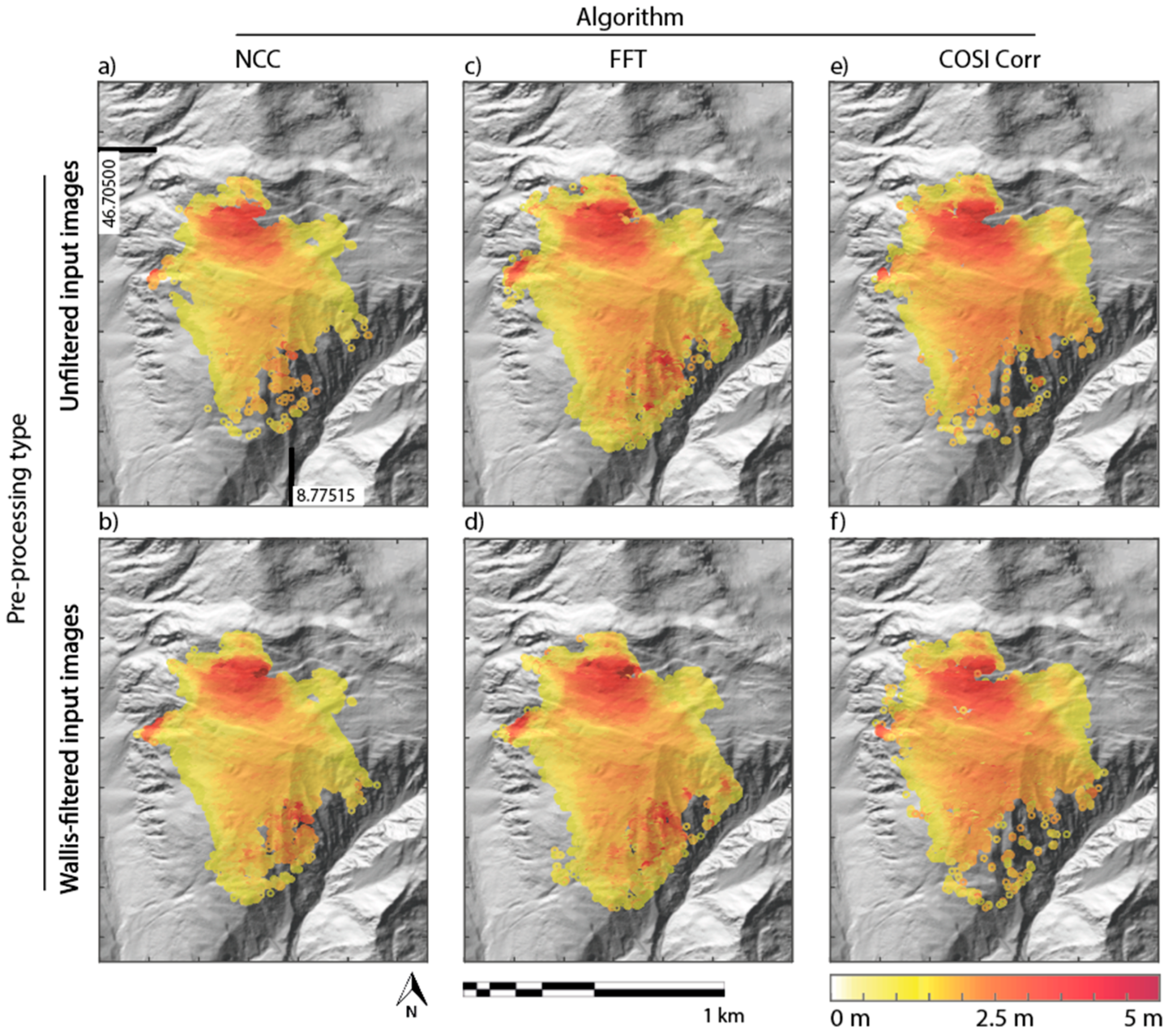
According to the DIC measurements, the major peak of the CdV deformation is situated in the North portions of the slope, with fringes extending towards the SE, W, and SW. The results show that data preprocessing has a significant impact on the correlation quality, and that all used algorithms have different abilities to represent the occurred displacement in the AoI over 16 years. The accumulated displacement measured by DIC over 16 years reaches up to 5 m. One example for the returned spatial coverage of the deformation field magnitude by each DIC algorithm is displayed in Figure 3), using original and preprocessed input image pairs as input. The used template size was 64 × 64 pixels, and all results have been filtered using the spatial vector operator. A zoom on details of the slope area towards the west is shown in Figure S3 in the Supplementary Material, which underlines quality differences in the returned displacement field, depending on the used code and the preprocessing.
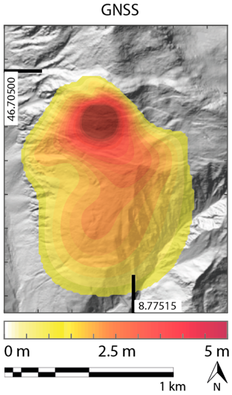
An interpolation of the derived GNSS displacement data from 23 measurement points across the AoI generally indicates a similar spatial deformation field and similar quantities as derived using DIC, while locally, the accumulated deformation exceeds 5 m. The resulting displacement field is illustrated in Figure 4.
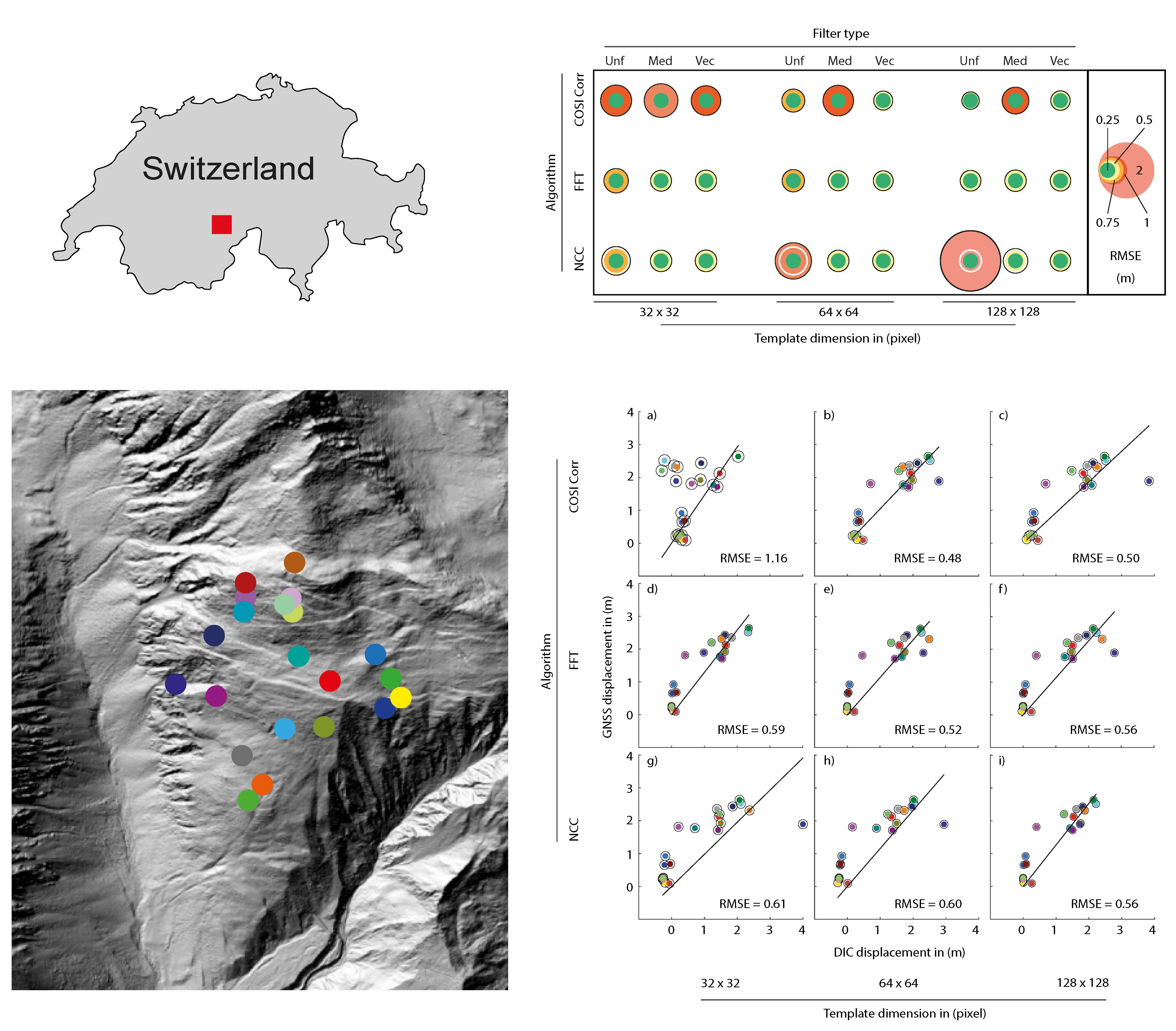
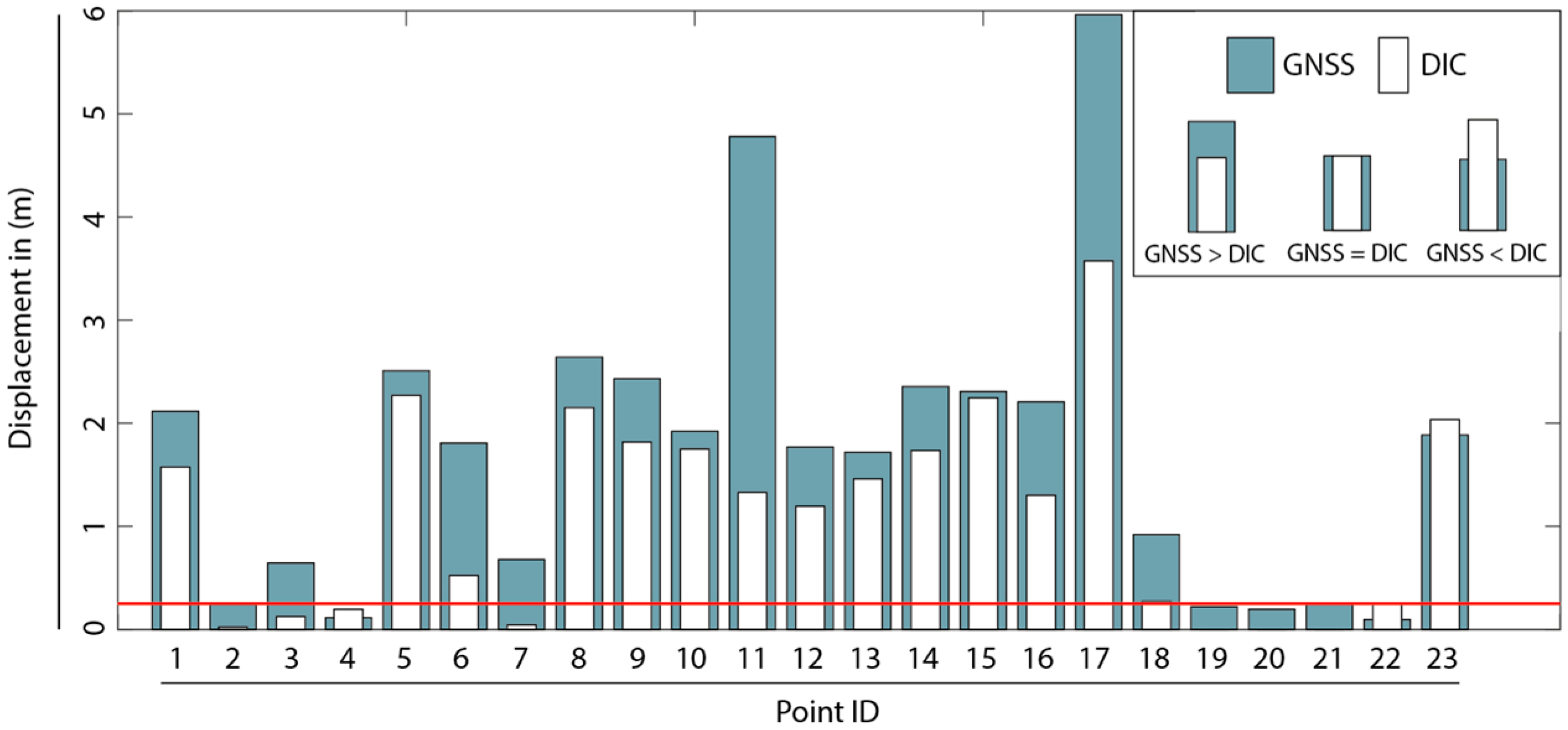
A direct quantitative comparison of the displacement at each measurement point as derived by DIC and GNSS shows good agreement. However, DIC measurements generally appear to slightly underestimate the true displacement throughout the AoI. In addition, for two measurement points (IDs 11 and 17) a substantial difference between DIC and GNSS of 3.5 and 2.5 m was identified (i.e., 14 and 10 pixels). The analysis of aerial imagery from the AoI suggests that there are no geomorphological features in the AoI that could explain the significantly different (i.e., larger) displacement values at these two monitoring points. Further, the patches of the DIC-derived displacement field in close vicinity to points 11 and 17 are not affected by noise. Although the discrepancy between the GNSS and DIC measurement has no obvious explanation, we considered these two GNSS measurement points as outliers, and discarded them from our further analysis.
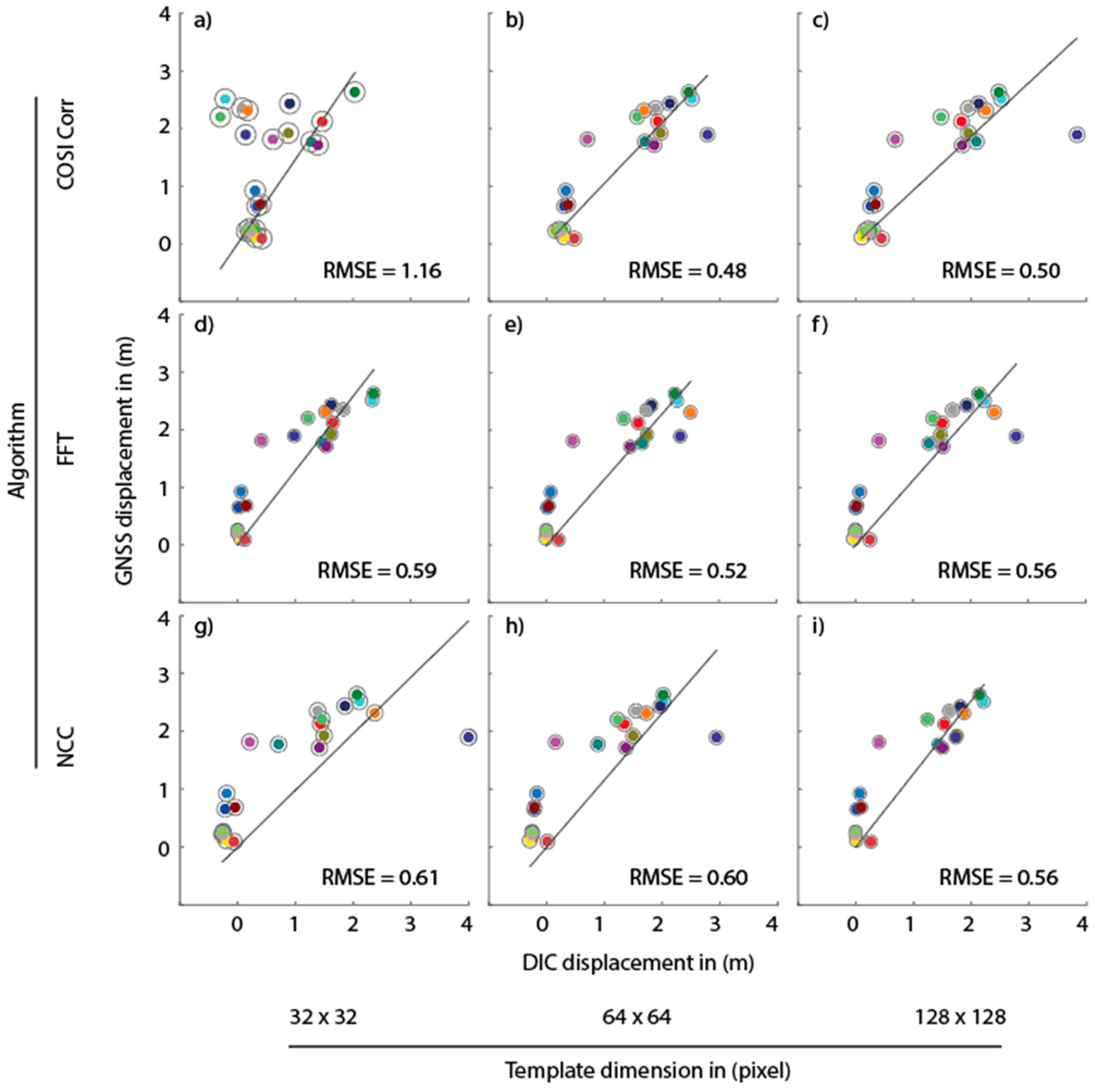
Figure 5 illustrates the comparison for a representative DIC run using a FFT-based correlator and a template size of 64 × 64 pixels, as well as a spatial vector operator. The GNSS-derived data has been plotted in grey color and in the background, while the DIC-derived data has been placed in the foreground and in white. Due to the similar quantitative performance of all assessed DIC codes, Figure 5 can be accounted as being representative for all conducted runs. The data further suggests that the minimum sensitivity of the applied algorithms is in the range of 25 cm or 1 pixel.
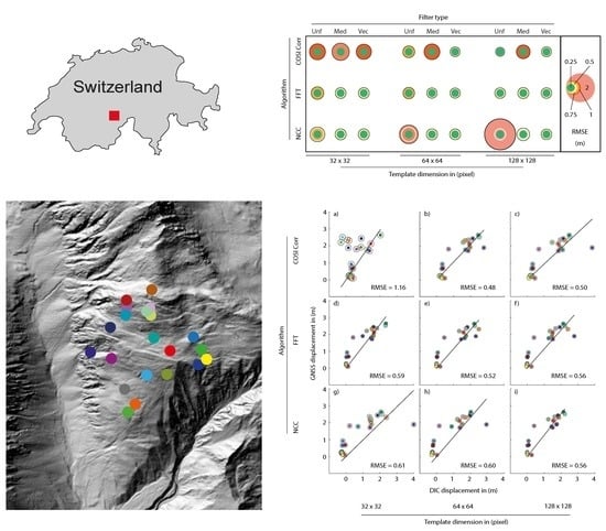
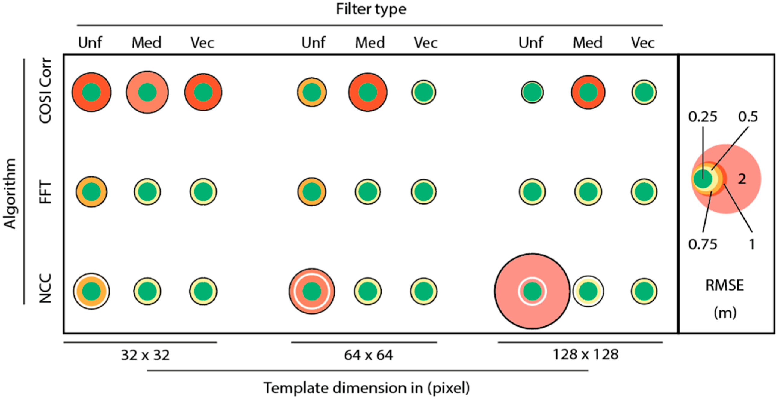
The quantitative analysis of 54 conducted DIC runs shows that the accuracy depends on the used algorithm, the input parameters, and the pre- and postprocessing procedures. The optimal performance is almost identical for all validated codes and is in the range of 0.5 m or 2 pixels. The results indicate that COSI Corr performs not as good as with small template sizes, while the other codes are relatively independent, particularly the FFT-based approach. An application of a Wallis filter does only have a relevant influence of the matching accuracy of the spatial-domain correlation code, but not on the frequency-domain codes. Postprocessing however, enhances the accuracy of all algorithms and template sizes, particularly if using a spatial vector operator. The overall accuracy of the assessed algorithms and setups ranges from 0.5 to more than 1 m, i.e., from 2 pixels to more than 4 pixels, depending on preprocessing treatment and on DIC processing parameters.
Figure 6 illustrates the quantitative comparison, using the size of the respective circle as an indicator for the achieved RMSE. The matrix represents runs with different template window sizes, ranging from 32 × 32 over 64 × 64 to 128 × 128 pixels, and using original as well as Wallis-filtered input imagery. In addition, the effect of no postprocessing, median filtering, and spatial vector filtering is displayed.
A comparison of the correlation error on a per-point-basis suggests that the inaccuracy of the displacement measurement with DIC is mainly caused by a general trend, rather than by isolated extreme mismatches. Further, the results of the analysis reveal differing capabilities of the used algorithms to match the image patches of master and slave around the GNSS measurement points. The velocity of the observed displacement does not seem to have an influence on the correlation accuracy, independent from the used DIC code. Figure 7 illustrates this analysis for selected runs. The horizontal rows represent the different algorithms, while the vertical rows represent template window sizes, ranging from 32 × 32 over 64 × 64 to 128 × 128 pixels.

5. Discussion

All three algorithms produce consistent results in terms of the spatial distribution of the displacement field. The DIC code based on a FFT approach returns the best spatial representation of the deformation field with the lowest contribution of noise, almost reaching a full coverage of the DSGSD (Figure 3c,d). The detection of displacements by DIC, in general, seems to be facilitated by applying an appropriate preprocessing to the input data. The contrast-enhanced images deliver results with less noise, less mismatches, and therefore, a better spatial coverage of the deformation field, particularly for NCC-based DIC algorithms (cf. 
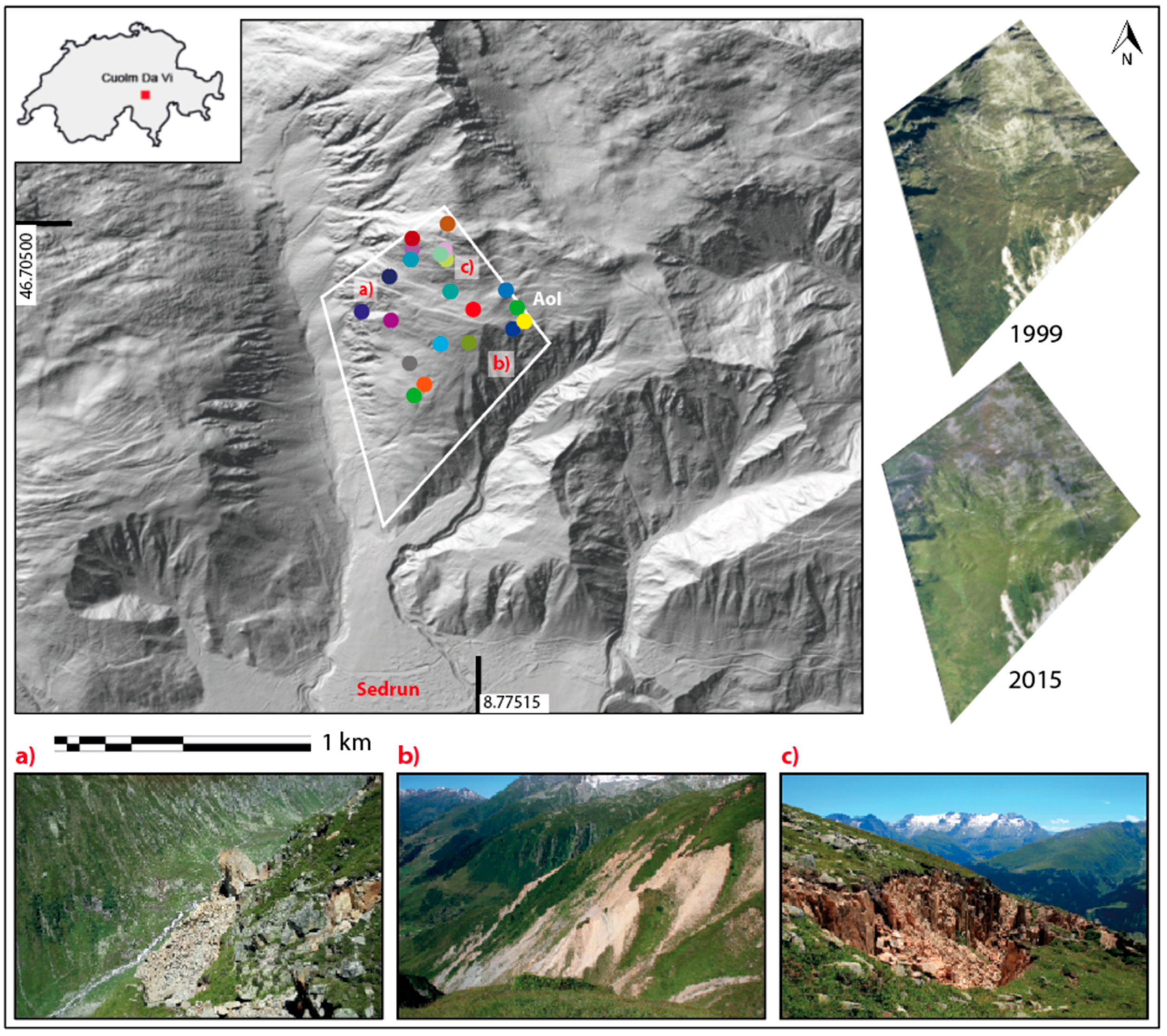
Figure S3). Contrast enhancement improves the matching quality even in areas with different shadow extents caused by different lighting conditions, as encountered in the NW of the CdV area. Parts of the slope in the northern peak area, as well as in the western displacement zone and in the southwestern ravine area show patches without data, as well as sharp contrasts in displacement; these regions are affected by noise, and were removed by the applied postprocessing filters. After field visits for ground-truthing, the most probable reasons for the noise level with respect to the extreme values at these locations, are correlator mismatches caused by illumination differences, changes in vegetation cover over the years, or the occurrence of failure-related rapid and non-linear surface changes, such as by erosion or shallow instabilities in the SE (cf. to Figure 1a–c) and Figures S1 and S2 in the Supplementary Material section for details).
The interpolated GNSS displacement map shows a similar deformation trend and spatial distribution of the displacement field as indicated by all DIC codes (Figure 4), and confirms the accumulated slope displacement of more than 5 m. The GNSS data reveals a single area with significantly larger displacements in the upper part of the slope towards the North. This is in contrast to the results derived with DIC, which indicate three hotspots: (1) in the area of the ravine in the SE; (2) in the northern part of the landslide (i.e., consistent with the area of larger displacements identified with GNSS); and (3) in the western part of the landslide on a slope towards the Val Strem. In the latter area, a major rock fall event occurred on 14 March 2016—roughly one year after the acquisition of the 2015 image used for this study—with an estimated volume of 2 × 10⁵ cubic meters [45]. The event caused damage to a small power plant within the valley and led authorities to restrict access to Val Strem until present. This illustrates a main advantage of the DIC technique, as displacements are measured over large areas and with quasi-full coverage, avoiding biases introduced by the selective placement of instrumentation or measurement points. If images are acquired regularly, DIC can be used to identify spatial and temporal variations of the deformation field, enabling the targeted application of countermeasures. An additional benefit is that the second hotspot area is located on a steep slope, which is difficult to access with GNSS. A remote measurement taken, e.g., by a UAV, is a much quicker and safer option, than, e.g., performing in situ GNSS measurements. A comparison of Figure 3 and Figure 4 also illustrates the finer spatial resolution of the DIC-derived deformation, which could be relevant for a precise assessment of the hazard potential of close-by infrastructures, in this case, the Parlet cable car station in the very East of the AoI.
For the quantitative assessment of the applied DIC methods, the twelve nearest-neighbors of each GNSS measurement point were extracted from the DIC derived deformation matrix (cf. Figure S4). Due to the relatively large spatial footprint of these twelve points, depending on the used scan window size and the search window movement pattern, the derived average of the deformation field might be biased, as the DIC codes sample the displacement over a larger area than is measured with the GNSS antenna, potentially considering areas with lower or higher deformation. In addition, the footprint might contain pixels, which are noise. Thus, in both cases, the accuracy of the respective extraction, and therefore, the accuracy of the entire assessment would be reduced. However, a trial and error approach has shown that this number of points delivers the best compromise between susceptibility to noise and accuracy, in direct comparison to an extraction of the single, four, or twenty-four closest points from the respective DIC deformation matrix. Still, the used extraction technique introduces a certain bias, which will generally lead to a slight underestimation of the actual accuracy of all applied DIC algorithms.
The quantitative assessment (Figure 6) shows that all applied algorithms predominantly achieve accuracies of around 50 cm (e.g., two pixels considering source imagery GSD), with significant differences in the quality of the spatial coverage, however. COSI Corr tends to achieve higher accuracies when using large search windows, opposite to the NCC-based algorithm. The FFT-based code performs with a constantly high accuracy over a broad range of template sizes (the code for the FFT-based routine is available on GitHub and MathWorks File Exchange, see Acknowledgements). Remarkably, the accuracy of COSI Corr drops significantly for smaller template dimensions, i.e., 32 pixels, confirming similar findings by [17,22]. A similar behavior cannot be observed for the other frequency domain based code using a FFT-correlator, however.
Ref. [33] proposed that DIC is capable to achieve subpixel accuracies for slope instability monitoring, but these results were not confirmed by an external source of displacement information, such as a GNSS dataset. Ref. [13] reports correlation accuracies within the range of 2 to 3 or more pixels for aerial e.g., [46], and roughly 0.2 to 1 pixels for satellite optical imagery e.g., [22]. In addition, Ref. [16] describes RMSEs of around 0.26 to 0.36 m using satellite optical imagery with a GSD of 0.5 m/pixel, validated against a small number of GNSS points. The results of our study therefore fit well into the findings of previous work, although different source data, as well as processing routines, have been applied. As generally discussed by [33], quantitative errors in DIC application could be caused by several factors, such as misfits in master and slave co-registration, the usage of different optical instruments and platforms (plane—UAV), platform attitude, orthorectification errors, inaccurate resampling, and the applied DIC technique, with respect to the input parameters. In addition, long temporal baselines (in our specific case 16 years) might negatively influence the correlation of the input images, thus affecting the DIC accuracy as well.
As indicated in Figure 6, a Wallis preprocessing does not have a significant influence on the accuracy of DIC, apart from the spatial domain algorithm that significantly benefits from the radiometric correction, as long as no postprocessing is applied. Generally, the application of postprocessing filters increases the performance of all tested DIC codes, particularly by using the spatial vector filter. If the applied template size is very large or if the used imagery has a very poor GSD, the vector filter routine could erroneously remove true surface displacements as noise, if the moving area is only represented by one or a couple of cells, and therefore, underrepresented within the local pixel neighborhood. In such a specific case, the application of no postprocessing filter is recommended to retain all information for interpretations.
The comparison of the DIC- and GNSS-derived displacement at each measurement point (Figure 7) indicates that the discrepancy of the measured deformation is not caused by isolated extreme values, but rather by general mismatching trends. The used algorithms appear to have correlation difficulties with different GNSS points, probably indicating a varying degree of susceptibility to radiometric differences by each code, depending on the method and domain of operation. Figure 7 further proposes that the accuracy of all DIC codes is independent of the magnitude of the observed displacement, i.e., slow movements are measured with the same accuracy as fast movements.
Some authors mention oversampling as a possibility to enhance the accuracy of the matching procedure [24,25]. For this study, three different methods of oversampling have been applied for the FFT-based and the NCC-based DIC algorithms. An increase of oversampling factor of both correlators has negligible effects. When oversampling the displacement field by using a template shift smaller than the Nyquist sample ratio, in this case, a quarter and an eighth instead of half of the applied template size, the RMSE remains at an equal level as well. It seems that the modified scan window sampling pattern, although producing a denser spatial representation of the deformation field, is not able to reduce the influence of noisy pixels or of true but non-representative displacements values of the surroundings. By applying DIC codes to up- or downsampled input images, i.e., over- or undersampled images using a factor of two, their accuracy reduces, particularly for the downsampled image. Probably the resampling and the associated blurring, with respect to averaging of the images, has a negative influence on the correlator, which also decreases the sensitivity of the algorithm. Generally, it has been found that oversampling has no influence on the quality of the returned displacement field, i.e., on the matching quality, nor has the noise level been increased. Still, oversampling has not been capable of enhancing the accuracy of DIC codes for the CdV case study, while increasing computational cost.
Besides the oversampling and the image pre- respectively post-processing, the search window size is a decisive parameter for DIC, as found during this study (cf. Figure 6), and as discussed by several authors [17,22]. Ref. [13,28] state that the dimensions of the template are a compromise between the desired accuracy of the displacement measurement and the spatial resolution of the displacement field. A larger template will facilitate the identification of matches while assuring a good signal-to-noise ratio (SNR), but the accuracy on the displacement estimates decreases because they are averaged over a larger correlation window. Therefore, the template size is a decisive parameter for DIC application, which is connected to the spatial resolution of the used input imagery, as well as to the magnitude of the expected deformation. The dimensions of the search window are normally related to the spatial extent of the template. A larger search window will slow down the correlation speed, as more matches have to be calculated, but enables the detection of larger displacements, in turn.
The optimal dimensions of the template window are tied to the GSD of the applied input imagery and to the magnitude of the observed deformation. Generally, as a theoretical initial guess, Ref. [47] recommend for COSI Corr to choose a template with a size of at least twice the expected deformation magnitude. In practice, they suggest the usage of a larger template however, within 8 to 17 times the expected deformation in pixels [47]. Using the results of this work with peak displacements of about 2.5 m, i.e., equal to 10 pixels, and with best results derived with templates of 64 × 64 and 128 × 128 pixels in size, the initial guess should be within 6 to 12 times the expected deformation. In addition, this study showed that this assumption is equally valid not only for COSI Corr, but also for the other two assessed DIC-algorithms, operating in the spatial as well as in the frequency domain. In consensus with [47], this study’s results suggests that the initial template size should be selected according to this formula
w i K · d e ,
with d e as the expected deformation, w i as the scan window size, both in pixels, and coefficient K varying between 6 and 17.
The findings suggest that sensors with a poorer spatial resolution cannot resolve slow landslide displacements, and that they need a larger temporal baseline to detect a slow displacement, assuming constant deformation over time. Cameras with a smaller GSD would be more efficient in the detection of similar displacements considering smaller temporal baselines. It is important to note that, in theory, sensors with large GSDs are capable of detecting the same surface deformations as cameras with small GSDs, if the temporal baseline is sufficiently long, or if the deformation rate of the observed instability is high enough. Yet, cameras with a large GSD will fail to identify displacements with a spatial footprint smaller than their spatial resolution, independent of the magnitude of the deformation. The recommendation for window size by [47], as well as the modification on behalf of the authors, still requires at least an estimate of the scale and magnitude of the expected slope instability deformation, which might be difficult or impossible to assume before. As observed surface displacements might be nonlinear, or only active under certain conditions, an application of DIC for instability monitoring can be further exacerbated, because the used input imagery must have a sufficient temporal baseline, which covers actual deformation with, at the same time, a potentially detectable speed of displacement. Therefore, the use of imagery with varying GSDs, e.g., images taken by a UAV from different altitudes above the slope instability, as well as the application of input data with varying temporal baselines in combination with differing template sizes, starting from the recommendations given by the discussed Formula (1), is proposed for a comprehensive detection and monitoring of slope instabilities.
Other limitations of DIC for slope monitoring are environmental conditions that impede the acquisition of optical imagery, such as fog, low clouds, or strong winds. As heavy rainfalls, and water, in general, have been identified as a main trigger of landslides [6], monitoring capabilities of DIC can be restricted by poor weather conditions, and the impossibility to fly UAVs. Further, using only nadir looking imagery from off-ground platforms, the monitoring of vertical displacements is not possible, significantly limiting the ability of DIC to directly monitor, e.g., the rotational component of slope instability. This limitation can be overcome using, e.g., UAVs and oblique acquisitions. In addition, advanced DIC approaches combining multiple viewing geometries could be used to retrieve 3D displacements of an active slope instability.
However, DIC in combination with off-ground sensors offers the possibility to derive fairly accurate and unbiased displacement measurements over large areas for comparably low costs. As the accuracy is dependent on the GSD, the application of UAVs flying repeatedly at low altitudes enables monitoring with very high accuracy and temporal resolution. In addition, observations in remote areas are possible, where direct access is denied by rough terrain or steep slopes.

6. Conclusions

This study showed that DIC applied to high-resolution optical imagery from an airborne sensor allows the detection and accurate monitoring of slow and fast coherent displacements of the CdV DSGSD over 16 years. All DIC codes have achieved peak accuracies and precisions around 50 cm or 2 pixels, while the FFT-based algorithm provided a significantly better spatial coverage of the instability, in combination with a particularly constant level of performance, independent of template size or pre- and postprocessing. Dynamic range enhancement and radiometric preprocessing significantly improves the deformation field coverage by DIC, even in regions with extremely different illumination, especially for codes operating in the spatial domain, while reducing the general noise level. Still, the accuracy of matching is only improved for spatial correlators without any applied postprocessing. Appropriate removal of noise by postprocessing filters, particularly by a newly developed spatial vector filter, proved to be capable of further improving the accuracy of all algorithms and in any situation. Still, DIC appeared to slightly underestimate the occurred true displacement, in a general trend. An oversampling during DIC or as preparation prior to DIC has not been found to improve the accuracy of spatial and frequency domain DIC codes in any way, nor has it been found to affect the noise level or the quality of the spatial coverage of the displacement field. By contrast, the over- or downsampling of the used input imagery resulted in worse results, probably caused by a blurring of the images, causing a systematic underestimation of the displacement field by spatial and frequency domain DIC codes.
The findings of this study confirm assertions from the literature that the used template window size is the decisive parameter for the effectiveness of DIC, and that it has to be carefully determined and altered. An initial guess can be based on the presented Equation (1). In general, the application of imagery with different spatial resolutions, as well as data with varying temporal baselines in combination with the application of varying template window sizes is recommended to optimize detection and monitoring of slope instabilities with DIC. In addition, the utilization of input image preprocessing involving a radiometric correction, e.g., a Wallis filter, as well as the application of postprocessing filters, e.g., using a spatial vector filter, is suggested to further enhance the accuracy and quality of the correlation.
The CdV case study has shown that DIC codes used on airborne optical imagery are reliable and capable of reaching high accuracies, while being able to monitor displacements on large or even regional scales, and over long timescales. At the same time, the derived deformation enables not only the monitoring of slope instabilities, but also the detection of yet unknown features, as demonstrated by the recognition of the significant displacement of CdV West, prior to failure on 14 March 2016. This information allows an adaptation or even the deployment of a respectively traditional in situ on-ground monitoring system, in order to maximize the capabilities to monitor a particular slope instability. Further, DIC, in combination with off-ground platforms, can facilitate the access to remote or dangerous areas, while providing an excellent cost/benefit ratio per measurement. These properties promote the utility of DIC in combination with off-ground optical high-resolution data for numerous applications, including landslide hazard observation.

Supplementary Materials

The following are available online at https://0-www-mdpi-com.brum.beds.ac.uk/2072-4292/10/6/865/s1, Table S1: GNSS measurement details, Figure S1: Orthorectified single band input image of the CdV AoI, taken in 1999. Figure S2: Orthorectified single band input image of the CdV AoI, taken in 2015. Figure S3: Zoom into the CdV displacement field as returned from the NCC-based code, the FFT-based code, and COSI Corr. Figure S4: Scheme of vicinity-point offset data extraction.

Author Contributions

V.T.B. and A.M. conceived and designed the experiments; V.T.B. performed the experiments and wrote the paper; V.T.B. and A.M. analyzed the data; F.A. provided information over the area of study; All the co-authors revised the manuscript.

Acknowledgments

The authors want to acknowledge the contribution of Andrea Wolter to the supervision of the MSc thesis that this study is based on. The authors gratefully acknowledge the indirect support by Urs Mall and the International Max Planck Research School at the Max Planck Institute for Solar System Research in Goettingen by enabling the work on this manuscript. The authors additionally acknowledge the supply of computational resources by Prof. Baltsavias and the Chair for Photogrammetry and Remote Sensing, Institute of Geodesy and Photogrammetry, Department of Civil, Environmental and Geomatic Engineering, ETH Zurich. The images for this study were provided by Swisstopo respectively Swissphoto, the Bonanomi AG, and the Donatsch & Partner AG. The GNSS time series from 1999 to 2015 has been provided by the Bonanomi AG and Donatsch & Partner AG. The described NCC and FFT algorithms were implemented in Matlab R2017a, including the pre- and postprocessing routines, as well as the statistical analysis of the deformation results. The COSI Corr release 10-23-14 has been used in combination with ENVI 5 Classic; results were transferred to Matlab R2017a for the statistical analysis. Data are available upon request to the authors. The FFT-based DIC algorithm as well as all described pre- and postprocessing routines are available under the MIT license at: https://github.com/bickelmps/DIC_FFT_ETHZ and https://de.mathworks.com/matlabcentral/fileexchange/67273-dic-fft-ethz.

Conflicts of Interest

The authors declare no conflict of interest. The founding sponsors had no role in the design of the study; in the collection, analyses, or interpretation of data; in the writing of the manuscript, and in the decision to publish the results.

Appendix A

Appendix A.1. Normalized Cross Correlation Approach (NCC)

The implemented normalized cross correlation algorithm operates in the spatial domain of the input images. Applications of NCC are versatile and widespread due to the simplicity of the code itself [22]. In this study, the Matlab R2017a built-in normxcorr2 code from the Image Processing Toolbox was utilized, which has been implemented using a formula from [48] with the correlation factor γ as
γ ( u , v ) = x , y [ f ( x , y ) f ¯ u , v ] [ t ( x u , y v ) t ¯ ] { x , y [ f ( x , y ) f ¯ u , v ] 2 x , y [ t ( x u , y v ) t ¯ ] 2 } 0.5 ,
with f as the image, t ¯ as the mean of the template, and f ¯ u , v as the mean of f(x,y) in the region under the template.
The algorithm computes the normalized cross correlation of a square template window from the older or master image and a square search window from the newer or slave image, with γ ranging from −1 (anti-correlation) to 1 (perfect match). During the processing, the template and the search window are simultaneously moved over the master and the slave [48]. Their shift is performed linewise (horizontally) and generally follows the Nyquist–Shannon sampling theorem. As the cross correlation is normalized, the comparison between images with different illumination angles is facilitated and the correlation coefficients from different correlation attempts can be compared [22]. The application of NCC is generally time intensive, as the code applies a spatial-domain convolution operation—a frequency domain-based code will outperform NCC [22]. Another potential disadvantage of NCC is mentioned by [22] as the inequality of occurring contrasts in the master and the slave. This means that the code could create erroneous matches if features in the image are changing non-systematically (e.g., irregular moving snow patches), as the code is looking for contrasts to perform the matching. High contrasts enhance image correlation, but high non-systematic intensity changes will confuse a NCC code. Ref. [15] further report correlation issues in areas with different moving characteristics, such as landslide boundary areas. Ref. [28] also name rotation of features in the time between two acquisitions as possible reason for matching failure, as NCC struggles to recognize rotation.

Appendix A.2. Fast Fourier Transform Approach (FFT)

The selected algorithm by [44] operates in the frequency domain and obtains an initial estimate of the cross-correlation peak between master and slave within moving square search windows using a fast Fourier transform. The shift estimation is refined by an upsampling of the discrete Fourier transform in a small neighborhood of that estimate by means of a matrix multiplication. By using this approach, all image points are used to calculate the upsampled cross correlation [44].
According to [22], FFT approaches generally perform faster than NCC-based routines, but do not transform a normalization to the frequency domain easily—this could cause mismatches if illumination conditions change during the acquisitions. A way to approximate normalization with FFT is to consider only the phase information of an image; this ignores the differences in the intensity of the images [22]. According to [22] the cross correlation CC is then expressed as
C C ( i , j ) = I F F T ( F 0 ( u , v ) G 0 * ( u , v ) | F 0 ( u , v ) G 0 * ( u , v ) | ) ,
with IFFT being the inverse of the discrete fourier transform, F(u,v) the FFT of the matching window from the image at time = 1, and G(u,v) the FFT of the matching window from the image at time = 2; * denotes a complex conjugate. Ref. [22] as well as [17] suggest that DIC codes operating in the frequency domain, such as FFT-based codes and COSI Corr, generally achieve worse matching quality on small window sizes compared to spatial-domain methods, such as the NCC.

Appendix A.3. Co-Registration of Optically Sensed Images and Correlation (COSI Corr)

The third used image matching code operates in the frequency domain as well and is called co-registration of optically sensed images and correlation (COSI Corr). This collection of algorithms and image processing codes is based on work by [33] and is distributed for free (for research) by the Caltech Tectonics Observatory on its webpage. It is implemented in ENVI, and has been developed with IDL (Interactive Data Language). In COSI Corr, the image registration and correlation is achieved with an iterative unbiased processor, which estimates the phase plane in the Fourier domain to detect subpixel shifts [33]. However, the estimated phase difference between master and slave is not transformed back to the spatial domain to find the maximum CC. By using a robust and iterative function for its measurements, COSI Corr is less sensitive to radiometric outliers [22]. COSI Corr uses a bell-shaped search window, which gives more weight to the inner part of the window than to the outer part, thus avoiding edge effects. By doing so, the misinterpretation of outliers within the search window—which could lead to erroneous results—is less probable. At the same time, pixels in the search window have to move very coherently for COSI Corr to retrieve a correct match—this could lead to problems in areas with incoherent deformations [22].

Appendix B

Appendix B.1. DIC Input Parameters

Appendix B.1.1. Search Window and Template Size

DIC algorithms consider a quadratic scan window of a specific size taken from the master image, called template, which is correlated within a larger search window placed onto the slave image [17]. During processing, the template is moving within the search window, while measuring the degree of radiometric correlation of the in-window pixel values between both template and search window. After completion of the template’s movement through the current search window, the search window skips to its new position, triggering a new scan with the template, until both input images have been scanned. The movement pattern of the template and of the search window is controlled by the same window skip factor.

Appendix B.1.2. Oversampling

In general, oversampling is the process of sampling a signal with a sampling distance smaller than the critical Nyquist distance or rate. In this work, the effect of oversampling on the accuracy and spatial coverage of the NCC and the FFT approach has been assessed in three different ways, by an oversampling through the DIC correlator itself, by an oversampling of the template shift, and by modifying the input images’ spatial resolution. The code operating in the spatial domain applies correlator oversampling by upsampling the spatial resolution of the template and the search window with a bicubic interpolation with a weighted average of pixels in the nearest 4-by-4 neighborhood. The frequency-domain correlator performs the same operation by increasing the precision of the image pair’s registration to a subpixel level [44]. Applied oversampling factors for this study were 4 and 8. Oversampling with an adapted template shift modifies the horizontal and vertical movement pattern of the scan windows, from the default Nyquist limit of half the template window size to smaller steps, causing a denser scan pattern. Here, the movement pattern has been modified using factors of 0.25 and 0.125, i.e., a fourth and an eighth of the template window size. The scaling of the input imagery is performed by a bicubic interpolation, just as performed by the NCC correlator, described above. Both, upsampling and downsampling have been performed with a factor of 2.

Appendix C

Appendix C.1. Data Preprocessing

Sub-optimal radiometric properties and the influence of varying lighting conditions can be improved by invoking a radiometric correction respectively a dynamic range optimization. This process is also called contrast or edge enhancement and has been performed using a Wallis filter. According to [43], this filter forces the local mean and contrast under a search window, which runs over the original image, to fit to some defined target values, which assures that different parts of the image have a similar dynamic range, thus facilitating matching. This operation is expressed as
f ( m , n ) = [ g ( m , n ) m g ] c * s f c s g + ( 1 c ) * s f + b m f + ( 1 b ) m g ,
with g and f as the original and the filtered image, m for the local mean, as well as s for the local standard deviation of the pixels within the window. c and b are, respectively, the contrast expansion constant and the brightness forcing constant. If the six input parameters are not carefully set, the dynamic range modification could also lead to negative effects, such as a saturation of pixels or to a disadvantageous distribution along the image histogram. In the best case, a post-filter histogram would have a Gaussian shape with no saturation at its ends.

Appendix C.2. Data Postprocessing

After invoking a DIC code, there are several possibilities to enhance the quality of the resulting deformation matrices by applying postprocessing methods, also referred to as output filters. In general, a filter tries to identify and delete data points from an image matrix that contain wrong or poor information. The developed vector filter operates in the spatial domain and assesses the DIC-derived deformation resultant, i.e., the magnitude and the direction of the measured offsets. The intention of the filter is to remove obviously noisy and wrong pixels, which are identified basing on their deviating direction and magnitude, in comparison to the average values of their immediate surrounding. These threshold values of the filter can be defined manually, or are connected to the search window size, which has been used during the preceding DIC run. If either the deviation in magnitude or direction of a correlation cell is larger than its respective threshold, the entire cell will be filtered out. The vector filter can be expressed in the form
x D e f _ f i l t , i j = | x D e f , i j a = 1 n x D e f n | c x ,
y D e f _ f i l t , i j = | y D e f , i j a = 1 n y D e f n | c y ,
m a g D e f _ f i l t , i j = | m a g D e f , i j a = 1 n m a g D e f n | c m a g ,
where c x , c y , and c m a g are the x, y, and magnitude threshold values, respectively, operating at image coordinates i and j. The DIC-derived deformation matrices have been compared to the GNSS (true) displacement in a quantitative sense. To do so, the values of DIC magnitude matrix closest to each of the 23 GNSS measurement locations were extracted and used for a quantitative comparison of the deformation. Following a trial and error approach, the utilization of the closest 12 DIC correlation cells around each single GNSS measurement point were identified best for the quantitative comparison, using the calculated RMSE of all options as an indicator. Twelve points achieve the best compromise between a good SNR and accuracy, as the displacement field is averaged over a larger area. Using only the closest point or closest 4 points proved to be very susceptible to noise, while not enhancing the accuracy of the comparison. Using the closest 24 points, however, decreased the accuracy, as the respective average is taken over too large of an area. The magnitude of the deformation, as determined by the GNSS network, was interpolated between the 23 measurements using an external Matlab R2017a function implemented by [49] called gridfit to enable a visual comparison of both techniques.

References

  1. Clague, J.J.; Roberts, N.J. Landslide hazard and risk. In Landslides; Clague, J.J., Stead, D., Eds.; Cambridge University Press: Cambridge, UK, 2012; pp. 1–9. ISBN 978-0-511-74036-7. [Google Scholar]
  2. EM-DAT|The International Disasters Database. Available online: http://www.emdat.be/ (accessed on 17 March 2018).
  3. De Blasio, F.V. Introduction to the Physics of Landslides; Springer: Dordrecht, The Netherlands, 2011; ISBN 978-94-007-1121-1. [Google Scholar]
  4. Landslides: Processes, Prediction, and Land Use. Available online: https://0-www-wiley-com.brum.beds.ac.uk/en-ch/Landslides%3A+Processes%2C+Prediction%2C+and+Land+Use-p-9781118665954 (accessed on 21 April 2018).
  5. Loew, S.; Gschwind, S.; Gischig, V.; Keller-Signer, A.; Valenti, G. Monitoring and early warning of the 2012 Preonzo catastrophic rockslope failure. Landslides 2017, 14, 141–154. [Google Scholar] [CrossRef]
  6. Korup, O. Landslides in the Earth system. In Landslides; Clague, J.J., Stead, D., Eds.; Cambridge University Press: Cambridge, UK, 2012; pp. 10–23. ISBN 978-0-511-74036-7. [Google Scholar]
  7. Manconi, A.; Giordan, D. Landslide failure forecast in near-real-time. Geomat. Nat. Hazards Risk 2016, 7, 639–648. [Google Scholar] [CrossRef]
  8. Mazzanti, P.; Bozzano, F.; Cipriani, I.; Prestininzi, A. New insights into the temporal prediction of landslides by a terrestrial SAR interferometry monitoring case study. Landslides 2015, 12, 55–68. [Google Scholar] [CrossRef]
  9. Manconi, A.; Kourkouli, P.; Caduff, R.; Strozzi, T.; Loew, S. Monitoring surface deformation over a failing rock slope with the ESA Sentinels: Insights from Moosfluh instability, Swiss Alps. Remote Sens. 2018, 10, 672. [Google Scholar] [CrossRef]
  10. Gabriel, A.K.; Goldstein, R.M.; Zebker, H.A. Mapping small elevation changes over large areas: Differential radar interferometry. J. Geophys. Res. Solid Earth 1989, 94, 9183–9191. [Google Scholar] [CrossRef]
  11. Barra, A.; Monserrat, O.; Crosetto, M.; Cuevas-Gonzalez, M.; Devanthéry, N.; Luzi, G.; Crippa, B. Sentinel-1 Data Analysis for Landslide Detection and Mapping: First Experiences in Italy and Spain. In Advancing Culture of Living with Landslides; Mikoš, M., Arbanas, Ž., Yin, Y., Sassa, K., Eds.; Springer International Publishing: Cham, Switzerland, 2017; pp. 201–208. ISBN 978-3-319-53486-2. [Google Scholar] [Green Version]
  12. Anuta, P.E. Spatial Registration of Multispectral and Multitemporal Digital Imagery Using Fast Fourier Transform Techniques. IEEE Trans. Geosci. Electron. 1970, 8, 353–368. [Google Scholar] [CrossRef]
  13. Delacourt, C.; Allemand, P.; Berthier, E.; Raucoules, D.; Casson, B.; Grandjean, P.; Pambrun, C.; Varel, E. Remote-sensing techniques for analysing landslide kinematics: A review. Bull. Soc. Géol. Fr. 2007, 178, 89–100. [Google Scholar] [CrossRef]
  14. Debella-Gilo, M.; Kääb, A. Sub-pixel precision image matching for displacement measurement of mass movement using normalised crosscorrelation. Remote Sens. Environ. 2011, 115, 130–142. [Google Scholar] [CrossRef] [Green Version]
  15. Cai, J.; Wang, C.; Mao, X.; Wang, Q. An Adaptive Offset Tracking Method with SAR Images for Landslide Displacement Monitoring. Remote Sens. 2017, 9, 830. [Google Scholar] [CrossRef]
  16. Stumpf, A.; Malet, J.-P.; Delacourt, C. Correlation of satellite image time-series for the detection and monitoring of slow-moving landslides. Remote Sens. Environ. 2017, 189, 40–55. [Google Scholar] [CrossRef]
  17. Rosu, A.-M.; Pierrot-Deseilligny, M.; Delorme, A.; Binet, R.; Klinger, Y. Measurement of ground displacement from optical satellite image correlation using the free open-source software MicMac. ISPRS J. Photogramm. Remote Sens. 2015, 100, 48–59. [Google Scholar] [CrossRef]
  18. Dehecq, A.; Gourmelen, N.; Trouve, E. Deriving large-scale glacier velocities from a complete satellite archive: Application to the Pamir–Karakoram–Himalaya. Remote Sens. Environ. 2015, 162, 55–66. [Google Scholar] [CrossRef] [Green Version]
  19. Euillades, L.D.; Euillades, P.A.; Riveros, N.C.; Masiokas, M.H.; Ruiz, L.; Pitte, P.; Elefante, S.; Casu, F.; Balbarani, S. Detection of glaciers displacement time-series using SAR. Remote Sens. Environ. 2016, 184, 188–198. [Google Scholar] [CrossRef]
  20. Casu, F.; Manconi, A. Four-dimensional surface evolution of active rifting from spaceborne SAR data. Geosphere 2016, 12, 697–705. [Google Scholar] [CrossRef] [Green Version]
  21. Manconi, A.; Casu, F. Joint analysis of displacement time series retrieved from SAR phase and amplitude: Impact on the estimation of volcanic source parameters. Geophys. Res. Lett. 2012, 39. [Google Scholar] [CrossRef] [Green Version]
  22. Heid, T.; Kääb, A. Evaluation of existing image matching methods for deriving glacier surface displacements globally from optical satellite imagery. Remote Sens. Environ. 2012, 118, 339–355. [Google Scholar] [CrossRef]
  23. Peppa, M.V.; Mills, J.P.; Moore, P.; Miller, P.E.; Chambers, J.E. Brief communication: Landslide motion from cross correlation of UAV-derived morphological attributes. Nat. Hazards Earth Syst. Sci. 2017, 17, 2143–2150. [Google Scholar] [CrossRef] [Green Version]
  24. Singleton, A.; Li, Z.; Hoey, T.; Muller, J.-P. Evaluating sub-pixel offset techniques as an alternative to D-InSAR for monitoring episodic landslide movements in vegetated terrain. Remote Sens. Environ. 2014, 147, 133–144. [Google Scholar] [CrossRef]
  25. Sun, L.; Muller, J.-P. Evaluation of the Use of Sub-Pixel Offset Tracking Techniques to Monitor Landslides in Densely Vegetated Steeply Sloped Areas. Remote Sens. 2016, 8, 659. [Google Scholar] [CrossRef]
  26. Darvishi, M.; Schlögel, R.; Bruzzone, L.; Cuozzo, G. Integration of PSI, MAI, and Intensity-Based Sub-Pixel Offset Tracking Results for Landslide Monitoring with X-Band Corner Reflectors—Italian Alps (Corvara). Remote Sens. 2018, 10, 409. [Google Scholar] [CrossRef]
  27. Manconi, A.; Casu, F.; Ardizzone, F.; Bonano, M.; Cardinali, M.; De Luca, C.; Gueguen, E.; Marchesini, I.; Parise, M.; Vennari, C.; et al. Brief communication: Rapid mapping of event landslides: The 3 December 2013 Montescaglioso landslide (Italy). Nat. Hazards Earth Syst. Sci. Discuss. 2014, 2, 1465–1479. [Google Scholar] [CrossRef]
  28. Travelletti, J.; Delacourt, C.; Allemand, P.; Malet, J.-P.; Schmittbuhl, J.; Toussaint, R.; Bastard, M. Correlation of multi-temporal ground-based optical images for landslide monitoring: Application, potential and limitations. ISPRS J. Photogramm. Remote Sens. 2012, 70, 39–55. [Google Scholar] [CrossRef]
  29. Scambos, T.A.; Dutkiewicz, M.J.; Wilson, J.C.; Bindschadler, R.A. Application of image cross-correlation to the measurement of glacier velocity using satellite image data. Remote Sens. Environ. 1992, 42, 177–186. [Google Scholar] [CrossRef]
  30. Chen, J.; Ke, C.; Zhou, X.; Shao, Z.; Li, L. Surface velocity estimations of ice shelves in the northern Antarctic Peninsula derived from MODIS data. J. Geogr. Sci. 2016, 26, 243–256. [Google Scholar] [CrossRef]
  31. Casu, F.; Manconi, A.; Pepe, A.; Lanari, R. Deformation Time-Series Generation in Areas Characterized by Large Displacement Dynamics: The SAR Amplitude Pixel-Offset SBAS Technique. IEEE Trans. Geosci. Remote Sens. 2011, 49, 2752–2763. [Google Scholar] [CrossRef]
  32. Ayoub, F.; Leprince, S.; Avouac, J.-P. Co-registration and correlation of aerial photographs for ground deformation measurements. ISPRS J. Photogramm. Remote Sens. 2009, 64, 551–560. [Google Scholar] [CrossRef]
  33. Leprince, S.; Barbot, S.; Ayoub, F.; Avouac, J.-P. Automatic and Precise Orthorectification, Coregistration, and Subpixel Correlation of Satellite Images, Application to Ground Deformation Measurements. IEEE Trans. Geosci. Remote Sens. 2007, 45, 1529–1558. [Google Scholar] [CrossRef] [Green Version]
  34. Walter, T.R.; Legrand, D.; Granados, H.D.; Reyes, G.; Arámbula, R. Volcanic eruption monitoring by thermal image correlation: Pixel offsets show episodic dome growth of the Colima volcano. J. Geophys. Res. Solid Earth 2013, 118, 1408–1419. [Google Scholar] [CrossRef] [Green Version]
  35. Bridges, N.T.; Ayoub, F.; Avouac, J.-P.; Leprince, S.; Lucas, A.; Mattson, S. Earth-like sand fluxes on Mars. Nature 2012, 485, 339–342. [Google Scholar] [CrossRef] [PubMed] [Green Version]
  36. Galland, O.; Bertelsen, H.S.; Guldstrand, F.; Girod, L.; Johannessen, R.F.; Bjugger, F.; Burchardt, S.; Mair, K. Application of open-source photogrammetric software MicMac for monitoring surface deformation in laboratory models. J. Geophys. Res. Solid Earth 2016, 121, 2852–2872. [Google Scholar] [CrossRef]
  37. Amann, F. Grosshangbewegung Cuolm Da Vi (Graubünden, Schweiz), Geologisch-geotechnische Befunde und numerische Untersuchungen zur Klärung des Phänomens. Ph.D. Thesis, FAU Erlangen-Nürnberg, Erlangen, Germany, 2006. [Google Scholar]
  38. Amann, F.; Donatsch, G.; Bonanomi, Y.; Moser, M. Kinematik und Bewegungsmechanismus der tiefgründigen Instabilität Cuolm Da Vi (Graubünden, Schweiz). Bull. Angew. Geol. 2006, 11, 117–131. [Google Scholar]
  39. Kleinbrod, U.; Burjánek, J.; Hugentobler, M.; Amann, F.; Fäh, D. A comparative study on seismic response of two unstable rock slopes within same tectonic setting but different activity level. Geophys. J. Int. 2017, 211, 1428–1448. [Google Scholar] [CrossRef]
  40. Swiss Geoportal. Available online: https://map.geo.admin.ch (accessed on 23 March 2018).
  41. Wang, Z.; Kieu, H.; Nguyen, H.; Le, M. Digital image correlation in experimental mechanics and image registration in computer vision: Similarities, differences and complements. Opt. Lasers Eng. 2015, 65, 18–27. [Google Scholar] [CrossRef]
  42. senseFly—eBee. Available online: https://www.sensefly.com/drone/ebee-mapping-drone (accessed on 23 March 2018).
  43. Baltsavias, E.P. Multiphoto Geometrically Constrained Matching. Ph.D. Thesis, ETH Zurich, Zürich, Switzerland, 1991. [Google Scholar]
  44. Guizar-Sicairos, M.; Thurman, S.T.; Fienup, J.R. Efficient subpixel image registration algorithms. Opt. Lett. 2008, 33, 156–158. [Google Scholar] [CrossRef] [PubMed]
  45. Val Strem Landslide: Natural Hazards. Available online: https://earthobservatory.nasa.gov/NaturalHazards/view.php?id=87818 (accessed on 4 April 2018).
  46. Delacourt, C. Velocity field of the “La Clapière” landslide measured by the correlation of aerial and QuickBird satellite images. Geophys. Res. Lett. 2004, 31. [Google Scholar] [CrossRef] [Green Version]
  47. Ayoub, F.; Leprince, S.; Keene, L. User’s Guide to COSI-CORR Co-registration of Optically Sensed Images and Correlation; California Institute of Technology: Pasadena, CA, USA, 2015; Volume 38. [Google Scholar]
  48. Lewis, J.P. Fast normalized cross-correlation. Vis. Interface 1995, 10, 120–123. [Google Scholar]
  49. D’Errico, J. Surface Fitting Using Gridfit—File Exchange—MATLAB Central. Available online: http://de.mathworks.com/matlabcentral/fileexchange/8998-surface-fitting-using-gridfit (accessed on 17 March 2018).
Figure 1. Cuolm da Vi (CdV) area of study overview; all global navigation satellite system (GNSS) measurement points are marked as color-coded dots on the hillshade. Letters (a) through (c) denote locations of particular interest: (a) local slope failure (14 March 2016); (b) ravine erosion and instability; and (c) tension cracks at the eastern margin of the landslide. RGB versions of the used input imagery are shown on the right. GNSS point color coding is described in Table S1 in the Supplementary Material. WGS 84. (Hillshade taken from [40]).
Remotesensing 10 00865 g001
Figure 2. Adopted workflow for this study; (1), (2), and (3) denote possibilities for oversampling, as described in the text.
Remotesensing 10 00865 g002
Figure 3. CdV displacement field returned from the normalized cross correlation (NCC)-based code (left column), the fast Fourier transformation (FFT)-based code (center), and COSI Corr (right); top row is based on original input imagery, the bottom row is based on Wallis-filtered data. Blank areas indicate portions of the slope with displacements below DIC accuracy or without information. All runs were performed with a scan window size of 64 × 64 pixels and a spatial vector filter. WGS 84. (Hillshade taken from [40].)
Remotesensing 10 00865 g003
Figure 4. Interpolation of the CdV displacement field based on the 23 GNSS measurements only. Blank areas indicate portions of the slope without information or with deformations below DIC accuracy. WGS 84. (Hillshade taken from [40]).
Remotesensing 10 00865 g004
Figure 5. Displacement derived with GNSS (grey, background) and with DIC (white, foreground) per measurement point ID within the CdV AoI, in meters. Red line marks the assumed minimal sensitivity of all assessed DIC codes at ~1 pixel, or 0.25 m. The underlying run has been performed with a FFT-based code, a scan window size of 64 × 64, and with a Wallis and spatial vector filter; the results can be accounted as being exemplary for all conducted DIC runs.
Remotesensing 10 00865 g005
Figure 6. Accuracy of 54 DIC runs based on their respective RMSE value; used scan window size varies from left (32 × 32 pixels) to right (128 × 128 pixels). The subcolumns display results derived with different postprocessing filters: Unf) unfiltered, Med) median filter, and Vec) vector filter. The top row represents COSI Corr, the center row an FFT approach, and the bottom row an NCC approach. The maximal extent of the displayed circle indicates the run’s RMSE, while internal white circles indicate runs whose accuracies were improved by Wallis filtering. Color coding underlines the RMSE with green colors indicating small errors, and red colors representing larger errors. The green centered circle indicates the assumed minimum sensitivity of the technique of around 0.25 m, or 1 pixel.
Remotesensing 10 00865 g006
Figure 7. Direct comparison of measured displacements measured with GNSS (vertical) and DIC (horizontal) at each measurement point in the CdV AoI. Each dot represents one measurement location, color-coding corresponds to Figure 1 (GNSS measurement points). The columns display usage of scan window sizes from 32 × 32 to 128 × 128 pixels; the rows represent different algorithms. Each run’s RMSE value is displayed. Circles around the individual measurement points indicate the standard deviation of the respective run. All runs were Wallis filtered and vector filtered.
Remotesensing 10 00865 g007
Table 1. Examples for digital image correlation (DIC) application.
Target TypeInput DataPlatformAuthor
LandslidesSAR imagerySatellite[15]
~~~[24]
~~~[25]
~~~[26]
~~~[27]
~Optical imagery~[16]
~~Airborne[23]
~~Ground-based[28]
Glacier/ice movementSAR imagerySatellite[19]
~Optical imagery~[18]
~~~[22]
~~~[29]
~Multispectral imagery~[30]
Active tectonics/volcanoesSAR imagerySatellite[31]
~~~[20]
~~~[21]
~Optical imagery~[17]
~~~[32]
~~~[33]
~Thermal imageryGround-based[34]
OtherOptical imagerySatellite[35]
~~Ground-based[36]

