Synthetic Aperture Radar Image Segmentation with Reaction Diffusion Level Set Evolution Equation in an Active Contour Model

Abstract

This paper presents a method for synthetic aperture radar (SAR) image segmentation by draing upon a reaction–diffusion (RD) level set evolution (LSE) equation. The well-known RD theory consists of two main parts: reaction and diffusion terms. We first constructed the reaction term using an energy functional, which integrates the gamma statistical distribution with region–edge information from SAR images that can simultaneously suppress speckle noise and drive the active contour toward the object boundaries. Then, we used partial differential equation-based LSE to solve the proposed energy functional. Finally, a diffusion term was introduced into the LSE to ensure stability of the level set function and regularize the segmented region. The experimental results of both simulated and real SAR images showed that the proposed model has good robustness against a speckle noise as well as higher segmentation efficiency and accuracy than some existing models.

1. Introduction

The synthetic aperture radar (SAR) imaging system is an advanced Earth-observation technology owing to its special acquisition ability at all times and under all weather conditions. According to the imaging mechanism of SAR, SAR images can be broadly categorized into two classes: low-resolution and moderately high-resolution images. The former is usually characterized by of intensity homogeneity due to the perfect reflectivity of a microwave, and the latter possess the property of intensity inhomogeneity from inadequate reflectivity of a microwave. Intensity inhomogeneity, which is caused by inherent speckle noise, has been a long-standing and challenging issue in the field of SAR image processing. In the past decades, SAR image segmentation technology has been widely and intensively researched as an important step in information extraction and automatic interpretation, and a variety of methods have been proposed. These proposed methods can be classified into many categories: (1) clustering-based methods such as the fuzzy c-means clustering algorithm [1], (2) threshold-based methods, including the Otsu algorithm [2], (3) specific theory-based methods, e.g., artificial neural network and deep learning, which are often applied to SAR image segmentation under complicated scenarios [3,4], (4) super pixel-based methods such as the multi-kernel joint sparse graph and multi-feature ensemble models [5,6], and (5) level set evolution (LSE)-based methods such as the active contour model (ACM) [7]. Of these existing methods, ACMs, which were first proposed by Kass et al. [8], have attracted increasing attention from researchers owing to its clear and simple representation. The basic idea of the ACM is to develop an initial curve to locate a meaningful target edge by minimizing the energy functional. This can produce accurate segmentation in the form of a smooth and closed contour. However, when the parametric ACM often called the Snake model) is considered as an example, handling the topological change in the evolution curve is difficult. In contrast, this problem can be solved utilizing the widely used geometric ACMs based on the level set method [9]. Therefore, in the present study, we focus on geometric ACMs for the level set formulation.

The existing geometric ACMs can be roughly divided into three classes: edge-, region-, and region–edge-based models. The edge-based models [10,11,12,13] often utilize an edge indicator such as an image gradient to locate the desired object boundaries. However, the image gradient loses its effect under the influence of weak edge and strong noise (e.g., speckle noise), resulting in incorrect segmentation. The region-based models [14,15,16,17,18,19,20,21,22,23] usually use a certain region descriptor such as texture, intensity, or statistical distribution, which drives the curve to distinguish each region of interest. Therefore, they have better robustness against weak edge and noise. The region–edge-based models [24,25,26] are hybrid models, which typically aim at identifying a target region by combining certain specific regions and edge information that guides the motion of an active contour. As a result, disjoint regions with similar properties can also be sliced into independent parts. The Ayed model, proposed by Ayed et al. [16,17], is one of the famous region-based models, but it does not work well for SAR images with intensity inhomogeneity because its average estimation formula assumes that the intensities of SAR images are statistically homogeneous in each region. Further, the local characteristics of the Ayed model also cause the evolution curve to fall into local minima. To solve this local-minimum problem, Shuai et al. [19] proposed a stationary global minimum-based ACM by integrating the gamma statistical distribution with a level set framework. However, this method still failed to segment SAR images with intensity inhomogeneity because their average estimation formulas are the same as those in the Ayed model. Further, this method suffered from the drawback of low computational efficiency. Marques et al. [21] proposed a G_A⁰ statistical distribution-based ACM in a level set framework. They first used the G_A⁰ distribution to describe the statistical properties of the processed SAR images. Then, an improved average estimation formula based on the Ayed model was used to drive the curve toward the object edge. Although this method performs well for SAR images that are both intensity homogeneous and inhomogeneous, it suffers from a boundary leakage phenomenon because this model is not convex. Feng et al. [24] presented a method of transforming the non-convex energy functional into a convex energy functional. They used the fast Split Bregman method, instead of the traditional level set method, to minimize the proposed energy functional. As a result, the segmentation accuracy improved. Tu et al. [25] proposed a convex ACM based on a ratio distance. The model was defined by a linear combination of the modified Chan–Vese model [15] and region-scalable fitting (RSF) energy model [18] in a level set framework. It exhibited good robustness to the intensity inhomogeneity of SAR images. However, the complexity of the proposed algorithm increased because of the introduction of the ratio distance [27]. Xia et al. [28] proposed a multiscale ACM with a nonlocal processing criterion. The active contour was driven by a comparison principle, which compared each pair of patch similarity inside and outside the contour using the Kullback–Leibler divergence [29] in a nonlocal manner. During the evolution process of the contour, the reinitialization method was employed to regularize the segmented region and ensure a stable LSE. However, the reinitialization process was quite complicated, expensive, and showed boundary leakage as a side effect. Although a multiscale strategy was used to reduce the complexity of the algorithm, it remained unsatisfactory. In short, a great challenge still exists to find an efficient method to resolve the problems of accuracy and efficiency in SAR image segmentation.

In the current paper, we propose an improved ACM by combining the reaction–diffusion (RD) theory and level set framework. Recently, the RD concept has been applied in optical and medical image segmentation [30] and the related classification of polarimetric SAR image [31]. However, to our knowledge, application of the RD method in SAR image segmentation has not been fully studied. Here, we explore a method using a combination of RD and LSE for solving the segmentation problem of SAR images. The RD theory consists of two main parts: reaction and diffusion terms [32]. In the present study, we first constructed the reaction term using the energy functional that integrates the gamma statistical distribution with the region–edge information of SAR images, which can simultaneously suppress the speckle noise and drive the evolution curve toward the desired boundaries. Then, we used a partial differential equation (PDE)-based LSE to minimize the proposed energy functional. Finally, to simultaneously regularize the segmented region and ensure stability of the level set function, we added a diffusion term to free the complex reinitialization process. Compared with the other methods, our proposed method not only robust to speckle noise but also improves the efficiency and obtains accurate segmentation result.

The remainder of this paper is organized as follows. Section 2 presents the analysis of the drawbacks of the Ayed model and introduces the proposed model. Section 3 discusses the characteristics of the proposed RD method and presents some experiments comparing simulated and real SAR images. Section 4 discusses the choice of the related parameter and the application scope of the proposed model. Section 5 concludes this paper.

2. Materials and Methods

2.1. Ayed Model

Let $I(x)$ be the intense SAR image to be segmented and $\mathsf{\Omega }$ be the image domain, which is defined in $\mathsf{\Omega }\subset R^2$. ${\{{\mathsf{\Omega }}_i\}}_{i=1}^N$ denotes a set of pairwise disjoint regions, which satisfy $\mathsf{\Omega }={\cup }_{i=1}^N{\mathsf{\Omega }}_i$ and ${\mathsf{\Omega }}_i\cap {\mathsf{\Omega }}_j=\varnothing ,\forall i\ne j$, where N refers to the numbers of the regions. The goal of the SAR image segmentation is to obtain a family of regions that are homogenous with respect to the image characteristics. In the method used by Ayed et al. [16,17], each region ${\mathsf{\Omega }}_i$ of the SAR image can be modeled by a gamma distribution of mean intensity $u_i$ and number $L$ of looks, i.e.,

$$P_{u_i,L}\left(I\left(x\right)\right)=\frac{L^L}{u_i\mathsf{\Gamma }\left(L\right)}{\left(\frac{I\left(x\right)}{u_i}\right)}^{L-1}{e}^{\frac{-LI\left(x\right)}{u_i}}$$

(1)

Assuming that $I(x)$ is independent of $I(y)$ for $x\ne y$, the segmentation problem is to find a set of regions $\widehat{\mathsf{\Omega }}$ that maximizes likelihood $PL\left(\mathsf{\Omega }|I\right)$.

$$\begin{array}{ll}\widehat{\mathsf{\Omega }}& =\arg \underset{\mathsf{\Omega }}{\max }PL\left(\mathsf{\Omega }|I\right)\\ & =\arg \underset{\mathsf{\Omega }}{\max }{\displaystyle \prod _{x\in {\mathsf{\Omega }}_1}{P}_{u_1,L}\left(I\left(x\right)\right)}\cdot \cdot \cdot {\displaystyle \prod _{x\in {\mathsf{\Omega }}_N}{P}_{u_N,L}}\left(I\left(x\right)\right)\end{array}$$

(2)

Maximizing likelihood $PL\left(\mathsf{\Omega }|I\right)$ is equivalent to minimizing $-\log PL\left(\mathsf{\Omega }|I\right)$. Then, combining Equation (1) and the computation in [33] yields the following expression:

$$-\log PL\left(\mathsf{\Omega }|I\right)=L\left({\sum }_{i=1}^N{a}_i\cdot \log u_i\right)+\tau$$

(3)

where $\tau$ is a constant. $u_i$ is estimated using the average of $I(x)$ inside region ${\mathsf{\Omega }}_i$, and $a_i$ represents the area of region ${\mathsf{\Omega }}_i$. Their expressions can be presented as

$$u_i=\frac{{\displaystyle {\int }_{{\mathsf{\Omega }}_i}I\left(x\right)dx}}{{\displaystyle {\int }_{{\mathsf{\Omega }}_i}dx}} \mathrm{and} a_i={\displaystyle {\int }_{{\mathsf{\Omega }}_i}dx},i=1,2\dots N$$

(4)

Considering $N=2$, Equation (3) can be transformed to minimize the following two-region segmentation criterion:

$${\mathsf{{\rm E}}}^{Ayed}={\sum }_{i=1}^2{a}_i\cdot \log u_i+\lambda {\displaystyle {\int }_{C}dx}$$

(5)

In Equation (5), the region term (the first term) drives contour $C$ to approach the boundaries of the object, and the length term (the second term) is added to smoothen the contour. Only when the contour is located at the target edges can energy ${\mathsf{{\rm E}}}^{Ayed}$ reach the minimum value. $\lambda >0$ is a weight parameter used to balance the above two terms. Using the level set formalism [34] to minimize Equation (5) yields the following variational formulation:

$$\frac{\partial \varphi }{\partial t}=\left[-\log \frac{u_2}{u_1}-I\frac{u_1-u_2}{u_1{u}_2}-\lambda div\left(\frac{\nabla \varphi }{\left|\nabla \varphi \right|}\right)\right]\left|\nabla \varphi \right|$$

(6)

where $div(\cdot )$ denotes the divergence operator and $\nabla (\cdot )$ denotes the gradient operator. $\varphi$ is the level set function that takes positive values inside the contour, negative values outside the contour, and zero on the object boundary. Theoretically, the Ayed model cannot effectively handle SAR images with intensity inhomogeneity mainly because $u_i$, which plays a key role in Equation (6), assumes that the intensities of the SAR images are statistically homogeneous in each region. To clearly demonstrate the limitations of Equation (6), a simple experiment is performed on a simulated SAR image with intensity inhomogeneity, which is generated by adding a multiplicative noise with gamma distribution to a pure image, as shown in Figure 1a. It consists of three objects: a double circle, a triangle, and a horseshoe-shaped object whose intensity changes from bright to dark. The white line represents the initial contour. In Figure 1b–e, the setting of parameter $\lambda$ is from small to large. We can observe that if $\lambda$ is small, the segmentation results contain many false alarms. However, when $\lambda$ is large, the contour is stuck in local minima, resulting in a boundary leakage phenomenon. Obtaining an accurate segmentation by tuning only parameter $\lambda$ appears to be impossible. To solve this problem, more complete statistical properties of the local intensities must be considered.

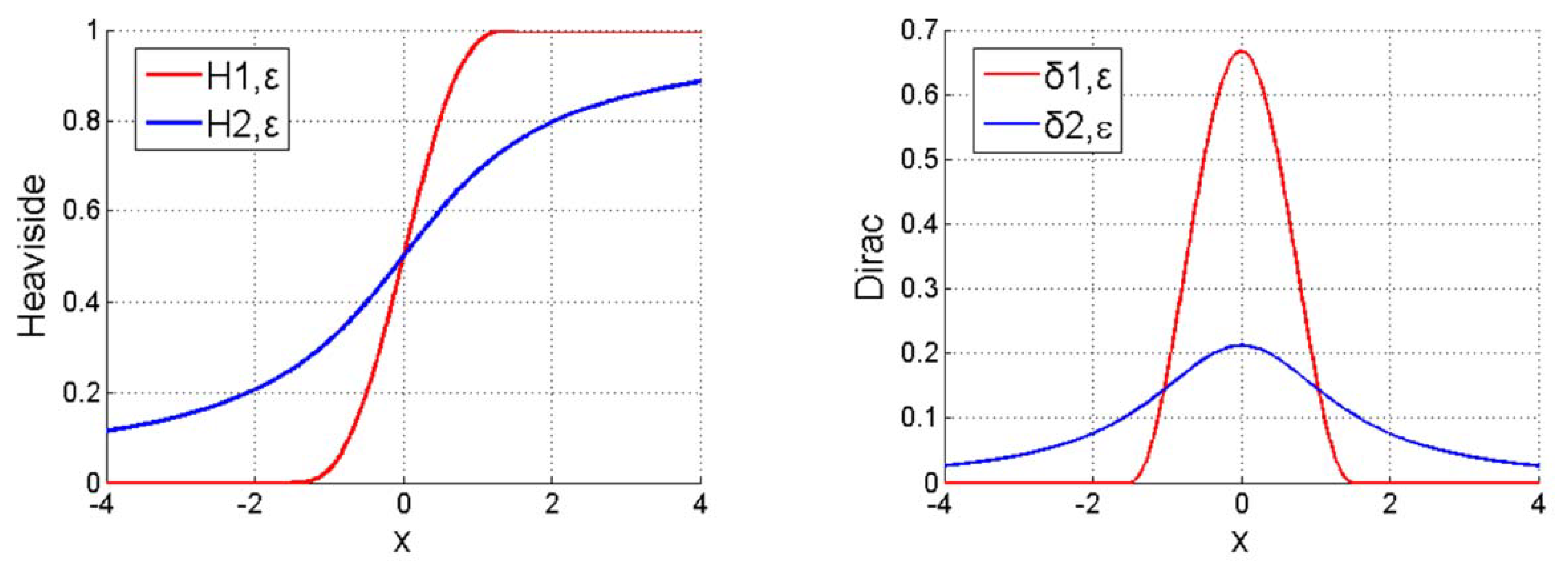
2.2. The Proposed Model

In this section, a reaction-diffusion level set evolution equation is proposed. The reaction term is derived by an improved energy functional based on the Ayed model, which can address the intensity inhomogeneity of SAR image. The diffusion term is introduced to regularize the segmented region and ensure stable level set evolution, thereby, overcoming the problem of boundary leakage and enhancing the segmentation efficiency.

In the medical image segmentation, we know that the classical RSF model can handle the images with intensity inhomogeneity effectively and its average estimate formula can be expressed as in [18],

$$f_i=\frac{K_{\sigma }(x)\ast \left[M_i(\varphi (x))I(x)\right]}{K_{\sigma }(x)\ast M_i(\varphi (x))},i=1,2$$

(7)

where $K_{\sigma }$ is a Gaussian kernel function with a standard deviation $\sigma$, and $M_1(\varphi (x))=H(\varphi (x))$, $M_2(\varphi (x))=1-H(\varphi (x))$ where $\varphi (x)$ is the level set function. $\ast$ is the convolution operator, and the convolution is utilized to smooth the image to suppress noise. In fact, the standard deviation $\sigma$ plays an important role in Equation (7). It can be seen as a scale parameter that controls the region-scalability from a small neighborhood to the whole image domain. As a result, more complete statistical properties of local intensities can be captured compared to Equation (4). However, we cannot simply use Equation (7) instead of Equation (4). First, it is necessary to investigate Equation (7). In the two-region case, the image domain $\mathsf{\Omega }$ can be segmented into two disjoint regions ${\mathsf{\Omega }}_1$ and ${\mathsf{\Omega }}_2$. In Equation (7), the regions ${\mathsf{\Omega }}_1$ and ${\mathsf{\Omega }}_2$ are represented with their membership functions defined by $M_1(\varphi (x))$ and $M_2(\varphi (x))$ [35], respectively. Different from Equation (7), we first use ${\eta }_i(x)$, which denotes the membership function of the region ${\mathsf{\Omega }}_i$. Then the $M_i(\varphi (x))$ of Equation (7) is replaced by a variable $\widehat{M}(\varphi (x))$ that can control the evolution of level set function $\varphi (x)$. Therefore, Equation (7) can be rewritten as

$${\widehat{f}}_i=\frac{{\displaystyle \int K_{\sigma }(x)\ast \left[\widehat{M}(\varphi (x))I(x)\right]}{\eta }_{i}dx}{{\displaystyle \int K_{\sigma }(x)\ast \widehat{M}(\varphi (x)){\eta }_{i}dx}},i=1,2$$

(8)

Here, ${\eta }_i$ meets the following requirements: ${\eta }_i(x)=0$ for $x\notin {\mathsf{\Omega }}_i$, and ${\eta }_i(x)=1$ for $x\in {\mathsf{\Omega }}_i$ ($i=1,2$) [35]. Thus, we can rewrite Equation (8) as

$${\widehat{f}}_i=\frac{{\displaystyle {\int }_{{\mathsf{\Omega }}_i}{K}_{\sigma }(x)\ast \left[\widehat{M}(\varphi (x))I(x)\right]}dx}{{\displaystyle {\int }_{{\mathsf{\Omega }}_i}{K}_{\sigma }(x)\ast \widehat{M}(\varphi (x))dx}},i=1,2$$

(9)

In Equation (9), the $\widehat{M}(\varphi (x))$ can be represented with the Heaviside function $H(\cdot )$ or delta function $\delta (\cdot )$, and their selection has an impact on the segmentation accuracy [30]. Usually, the Heaviside function $H(\cdot )$ can be approximated by the following two forms:

$$H_{1,\epsilon }(x)=\{\begin{array}{ll}\frac{1}{2}\left(1+\frac{x}{\epsilon }+\frac{1}{\pi }\sin \left(\frac{\pi x}{\epsilon }\right)\right),& \left|x\right|\le \epsilon \\ 1,& x>\epsilon \\ 0,& x<-\epsilon \end{array}$$

(10)

$$H_{2,\epsilon }(x)=\frac{1}{2}\left[1+\frac{2}{\pi }\arctan \left(\frac{x}{\epsilon }\right)\right],x\in R$$

(11)

The derivative of $H_{1,\epsilon }(x)$ and $H_{2,\epsilon }(x)$ are Dirac delta functions ${\delta }_{1,\epsilon }(x)$ and ${\delta }_{2,\epsilon }(x)$, respectively,

$${\delta }_{1,\epsilon }(x)=\{\begin{array}{ll}\frac{1}{2\epsilon }\left[1+\cos \left(\frac{\pi x}{\epsilon }\right)\right],& \left|x\right|\le \epsilon \\ 0,& \left|x\right|>\epsilon \end{array}$$

(12)

$${\delta }_{2,\epsilon }(x)=\frac{1}{\pi }\cdot \frac{\epsilon }{{\epsilon }^2+x^2},x\in R$$

(13)

where $\epsilon$ is a constant, if $\epsilon$ is too small, e.g., $\epsilon =0.5$, the value of ${\delta }_{2,\epsilon }(x)$ tends to be zero to make its effective range small, so the object may fail to be extracted if the initial contour is far from it. However, if $\epsilon$ is large, e.g., $\epsilon =2.5$, although ${\delta }_{2,\epsilon }(x)$ tends to obtain a global minimum, the final contour location may not be accurate. Here, the value of $\epsilon$ can be set as $\epsilon =1.5$ [13,18,26]. Moreover, we can see from Figure 2 that $H_{1,\epsilon }(x)$ and $H_{2,\epsilon }(x)$ are two monotone increasing functions, and the ${\delta }_{1,\epsilon }(x)$ and ${\delta }_{2,\epsilon }(x)$ are two convex functions. $H_{1,\epsilon }(x)$ has no maximum and minimum on the entire real number field. The support of $H_{1,\epsilon }(x)$ and ${\delta }_{1,\epsilon }(x)$ is restricted to a neighborhood of 0 so that the variable $x$ can only act locally. Hence, the curve tends to fall into local minima. In contrast, ${\delta }_{2,\epsilon }(x)$ acts on the entire real number field, which makes it easy to yield a global minimum [15].

Therefore, based on the above analysis, the proposed average estimate formula can be defined as,

$$c_i=\frac{{\displaystyle {\int }_{{\mathsf{\Omega }}_i}{K}_{\sigma }(x)\ast \left[{\delta }_{2,\epsilon }(\varphi (x))I(x)\right]}dx}{{\displaystyle {\int }_{{\mathsf{\Omega }}_i}{K}_{\sigma }(x)\ast {\delta }_{2,\epsilon }(\varphi (x))dx}},i=1,2$$

(14)

where ${\mathsf{\Omega }}_1$ and ${\mathsf{\Omega }}_2$ denote object region and background region, respectively. Moreover, we used an edge indicator function $g$ by

$$g=\frac{1}{1+|\nabla K_{\sigma }(x)\ast I(x)|}$$

(15)

where $g$ has the effect of accelerating the contour convergence because it usually takes smaller values at target boundaries than other locations [13]. Thus, combining the region term (Equation (14)) and the edge term (Equation (15)), Equation (5) can be rewritten as,

$${\mathsf{{\rm E}}}^O={\sum }_{i=1}^{2}g{\upsilon }_i\log c_i+\alpha {\displaystyle {\int }_{C}gdx}$$

(16)

where ${\upsilon }_i$ denotes the denominator of $c_i$ and $\alpha >0$ is a weight parameter to balance the two terms. Equation (16) can be seen as the reaction term which can suppress the speckle noise and drive the curve towards the desired boundaries. Then, the PDE-based LSE is used to minimize Equation (16), we obtain the following LSE equation (see Appendix A for detail derivation)

$$\mathsf{\Gamma }(\varphi )=-\left(e_2\log \frac{c_1}{c_2}+\frac{e_1}{c_1}-\frac{e_1}{c_2}\right)g\left|\nabla \varphi \right|-\alpha div\left(g\frac{\nabla \varphi }{\left|\nabla \varphi \right|}\right)\left|\nabla \varphi \right|$$

(17)

where $e_1=K_{\sigma }(x)\ast \left[{\delta }_{2,\epsilon }(\varphi (x))I(x)\right]$ and $e_2=K_{\sigma }(x)\ast {\delta }_{2,\epsilon }(\varphi (x))$. Generally speaking, the reinitialization method can be introduced into Equation (17) in order to ensure stable LSE. However, this method is quite complicated and has the side effect of boundary leakage (see Figure 3c). Fortunately, the Laplacian operator can solve this problem which has been demonstrated in [33,36]. Therefore, instead of the reinitialization process, we introduced a diffusion term “$\omega g\Delta \varphi$” into the LSE Equation (17), and the final RD LSE equation can be expressed as

$$\frac{\partial \varphi }{\partial t}=\omega g\Delta \varphi +\frac{1}{\omega }\mathsf{\Gamma }(\varphi )$$

(18)

where $\omega$ is a small positive constant, because when $\omega$ is large, $1/\omega$ is small which may weaken the effect of the reaction term $\mathsf{\Gamma }(\varphi )$, resulting in the risk of moving the active contour away from the object location. Therefore, we should use a small enough $\omega$ so that the active contour can extract the region of interest. $\Delta (\cdot )$ is the Laplacian operator. Equation (18) can be simply implemented by means of the finite difference method. The iterative procedure of the proposed algorithm is described below (Algorithm 1):

Algorithm 1 Proposed algorithm for SAR image segmentation

Input: a SAR image $I$, initialization $\varphi$, parameters $\omega ,\sigma$ and $\alpha$; Output: a segmentation $S$ 1: Initialization: iteration number $k\leftarrow 0$; ${\varphi }^0\leftarrow {\varphi }_0$; 2: for each pixel $x\in I(x)$ do 3:  Update local means $c_i$ using Equation (14); 4:  Update the level set function $\varphi$ using Equation (18); 5:  if $\varphi$ satisfies stationary condition, stop; otherwise, return to Step 2; 6: end for

2.3. Computational Complexity Analysis

In this section, we analyze the computational complexity of the proposed model. Supposing that the number of iterations is $k$ and the size of the processed SAR image is $m$. The size of the Gaussian kernel can be truncated as an $\vartheta \times \vartheta$ mask for efficiency, where $\vartheta$ is a positive integer. Then, the Gaussian kernel function divide the processed image into $n$ blocks [21,28], i.e., $m/{\vartheta }^2=n$. Thus, the time complexity of the proposed method can be denoted by $O(nk)$. Since the method of [17] does not use the Gaussian kernel, its time complexity is $O(mk)$. Moreover, Marques et al. [21] has to estimate three unknown parameters by using an extra estimation algorithm in each iteration, so its time complexity is $O(nk+\theta k)$, where $\theta$ indicates computational complexity of the estimation method in each iteration. Compared with [17,21], the reinitialization method was employed to regularize the segmented region and ensure a stable LSE in [28], so the time complexity of [28] is $O(n^{2}k)$ which is higher than that of the proposed method.

3. Results

We performed the segmentation using the proposed model on some simulated and real SAR images, and the results were compared to some existing models. Unless otherwise specified, we used the following parameters: $\omega =0.25,\sigma =6,\alpha =0.02$ and time step $\Delta t=0.01$. Our code was implemented in Matlab R2014a and run on a laptop with an Intel Core i7 at 3.3 GHz, and the timings are given in seconds (s).

3.1. The Effect of Proposed RD Term

We first discuss the effect of the proposed RD term and make a comparison between the reinitialization method and the diffusion term for airborne SAR data, as shown in Figure 3. Figure 3b shows the segmentation result of Equation (17). It can be seen that there is edge leakage at the location of the narrow street (see the green arrow in Figure 3b). This fault is caused by intensity inhomogeneity, resulting in the instability of LSE. Usually, in order to ensure a stable LSE, the reinitialization method is introduced into Equation (17). However, we can see from Figure 3c that a worse result is obtained compared to Figure 3b. This is mainly because when the reinitialization process is utilized to regularize the level set function, it also spontaneously suppresses the appearance of the new contours [30]. In contrast, the diffusion term can solve the problem, and an accurate segmentation result is achieved, as shown by Figure 3d.

Next, our proposed model is inspired by the two-step splitting method (TSSM) [30] which has been successfully applied in noise image segmentation. Therefore, it is necessary to make a comparison between these two methods. Note that, for a fair comparison, we used the default setting of the parameters and two original noise images in [30], and the iteration numbers are set as 3000. We can see from Figure 4 that the proposed method obtains more accurate segmentation results than the TSSM in the same initial contours, and the corresponding final level set functions of the proposed method (see Figure 4f,h) are smoother than the results of the TSSM (see Figure 4e,g).

3.2. Robustness to Speckle Noise

In order to demonstrate the capability of the proposed method in dealing with speckle noise, we tested our method for two different, real SAR images, as shown in Figure 5: a $433\times 433$ sub-image of the oil spill from an ENVISAT ASAR image (see the upper left of Figure 5), with a spatial resolution of 30 m, and a $512\times 512$ image of a river from an ALOS PLASAR (see the lower left of Figure 5), with a spatial resolution of 6.25 m. The three blue solid lines on the right represent the respective intensity statistics of three blue solid lines in two SAR images (see the figure on the left in Figure 5). It can be seen that, when the spatial resolution is low, the change in the intensity is gentle which is characteristic of intensity homogeneous. However, when the spatial resolution is high, strong reflectors and textures are presented, making the intensity fluctuate severely (see the lower right of Figure 5), resulting in the statistical property of the local region being inhomogeneous. This is why the method in [17,19] cannot effectively SAR images with intensity inhomogeneity. Figure 6 shows the final segmentation result of the proposed model. We can see that our method has good robustness to speckle noise and obtains satisfactory results for the two real SAR images.

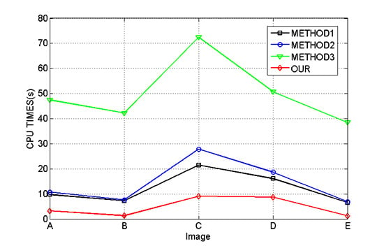
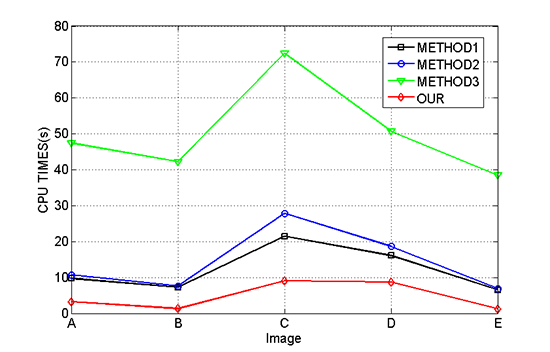
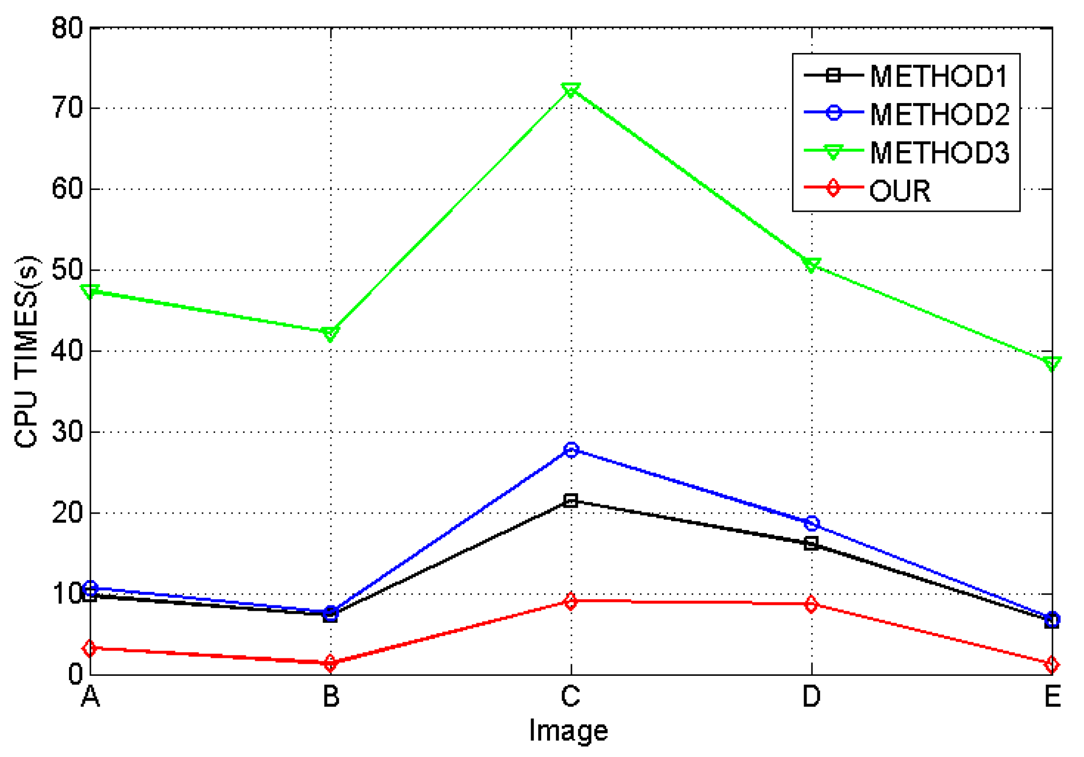
3.3. Comparison with the Existing Methods

We compared our method with three major approaches: the methods of Ayed et al. [17], Marques et al. [21] and Xia et al. [28]. For the sake of elaboration, we call these three methods METHOD1, METHOD2 and METHOD3, respectively.

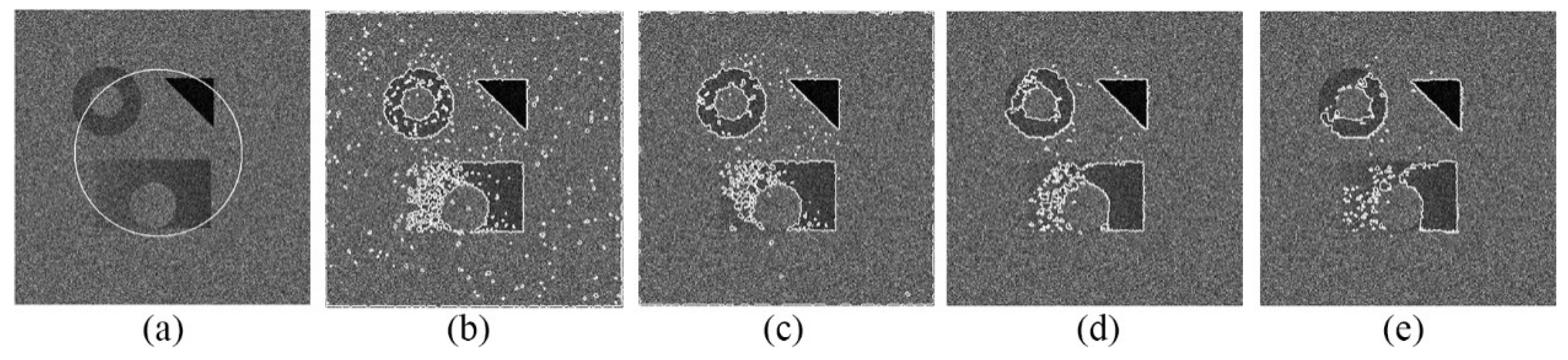
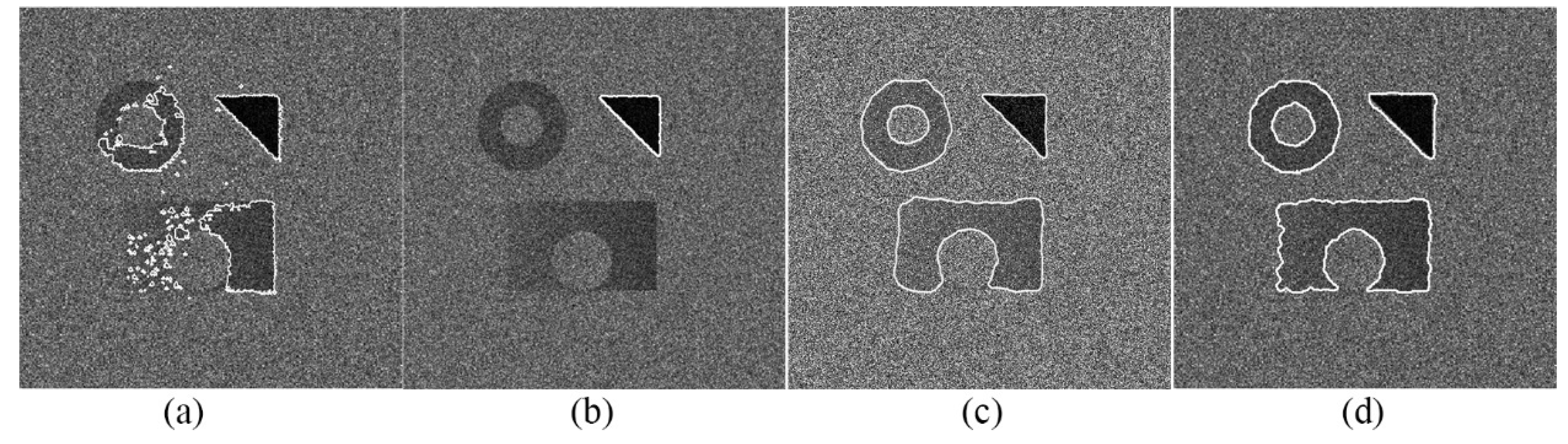
3.3.1. Results for Simulated SAR Image

In this section, in order to quantify the performance of the segmentation algorithms, we used the measuring method of [21], that is, difficulty of segmentation (DoS) and cross-region fitting (CRF). Firstly, the mathematical formula of the DoS can be expressed as

$$DoS=\frac{1}{S_{AG}(U_f,U_b)}$$

(19)

where $S_{AG}(U_f,U_b)$ is the arithmetic-geometric distance, and its expression is given by

$$S_{AG}(U_f,U_b)=\frac{1}{2}{\displaystyle {\int }_{R^{+}}\left[\left(P_{c_1,L}(I(x))+P_{c_2,L}(I(x))\right)\times \log \left(\frac{P_{c_1,L}(I(x))+P_{c_2,L}(I(x))}{2\sqrt{P_{c_1,L}(I(x))\times P_{c_2,L}(I(x))}}\right)\right]}dx$$

(20)

where $U_f$ and $U_b$ denote the foreground and background region, respectively. $P_{c_i,L}(I(x))$ is the Equation (1) and the expression of its subscript $c_i$ is Equation (14). Actually, the DoS quantifies the difficulty of segmenting the foreground and background. The lower the region contrast is, the higher the value of the DoS is. Thereby, the segmentation difficulty increases.

Then, we used the CRF to quantify the ability of the methods to partition object regions correctly. Its expression is given by

$$CRF=\frac{1}{1+\sqrt{DoS\times \left|S_{AG}\left(U_f^r,U_b^s\right)-S_{AG}\left(U_f^s,U_b^r\right)\right|}}$$

(21)

Here, $U_f^r$ and $U_b^s$ denote the reference region of the foreground and the segmented region of background, respectively. In contrast, $U_f^s$ and $U_b^r$ denote the segmented region of the foreground and the reference region of the background, respectively. When the value of CRF is closer to 1, it implies that the segmentation accuracy of the method is higher. The numerical results in

Table 1. DoS (difficulty of segmentation) and CRF (cross-region fitting) for the simulated SAR image in Figure 7.

d				CRF
L (Number of Looks)	Region	DoS	METHOD1	METHOD2	METHOD3	OUR
	double circle	5.6674	0.4233	-	0.8807	0.8922
3	triangle	2.7364	0.8607	0.9331	0.9282	0.9213
	horseshoe-shaped	10.9177	0.3087	-	0.8215	0.8763
	double circle	3.7632	0.4922	-	0.8361	0.8527
8	triangle	2.1053	0.8978	0.9427	0.9379	0.9307
	horseshoe-shaped	7.5239	0.3826	-	0.8533	0.8895

show that the proposed method not only has the best performance for different difficulty levels but also has superior separability of regions for different object contrast levels. Moreover, Figure 7 shows the segmentation results by METHOD1, METHOD2, and METHOD3 and our method for a stimulated SAR image with intensity inhomogeneity, and the initial contour as shown by Figure 1a. We can observe from Figure 7 that METHOD1 yields unsatisfying result due to the influence of speckle noise and weak edge. METHOD2 can only segment one target from the three. Although METHOD3 can extract all of the objects, it fails to locate the detailed information of the object boundary due to the fact that the complex reinitialization method is used to ensure the stable LSE. In contrast, we used the diffusion term to replace the expensive reinitialization process. As a result, correct segmentation was achieved, as shown in Figure 7d.

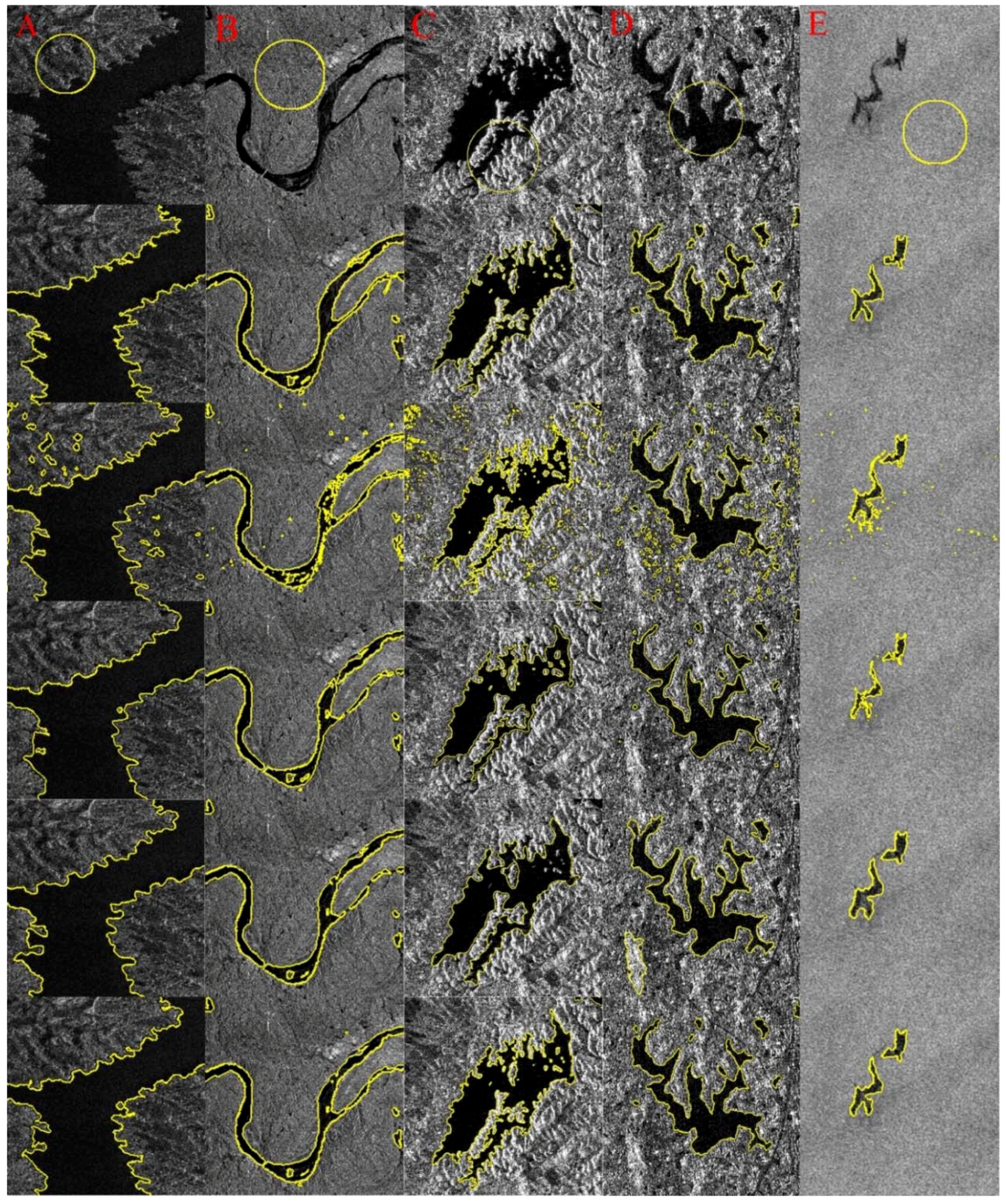
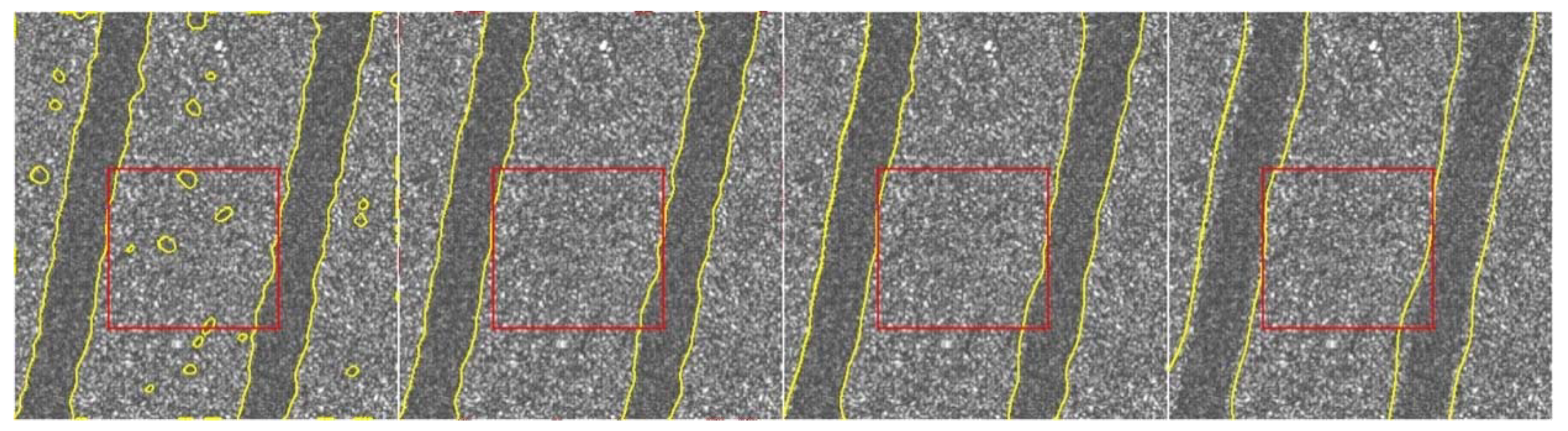
3.3.2. Results for Real SAR Image

We also evaluated the performance of the proposed method on different real SAR images which came from different SAR sensors. Detailed information for each SAR image can be observed in

Table 2. Comparison of region fitting error (RFE) scores for METHOD1, METHOD2, METHOD3 and our method.

Image (Pixels)	Sensors	Resolution	Objects	METHOD1	METHOD2	METHOD3	OUR
A ($362\times 362$)	RADARSAT	8 m	River	0.3761	0.2202	0.1430	0.1375
B ($256\times 256$)	TerraSAR	16 m	River	0.4028	0.1245	0.1379	0.0984
C ($500\times 500$)	ALOS PALSAR	6.25 m	Lake	0.5212	0.1754	0.2987	0.1274
D ($400\times 400$)	ALOS PALSAR	6.25 m	Lake	0.4941	0.1927	0.2063	0.1161
E ($250\times 250$)	ENVISAT ASAR	30 m	Oil spill	0.2716	0.1126	0.0933	0.0813

. The first row to the last row in Figure 8 represent the original SAR images and initial contours, the ground truth, the segmentation results of METHOD1, METHOD2, METHOD3 and the proposed method, respectively.

Moreover, we used the region fitting error (RFE) in [27] to quantitatively evaluate the segmentation accuracy of the proposed method by comparing it with METHOD1, METHOD2 and METHOD3. RFE is defined as follows,

$$\mathrm{RFE}(\mathsf{\Omega })=\frac{{\left|\mathsf{\Omega }\cup {\mathsf{\Omega }}_{\mathrm{g}}\right|}_{card}-{\left|\mathsf{\Omega }\cap {\mathsf{\Omega }}_g\right|}_{card}}{{\left|{\mathsf{\Omega }}_g\right|}_{card}}$$

(22)

where $\mathsf{\Omega }$ denotes the object region found by the method, ${\mathsf{\Omega }}_g$ represents the ground truth which is annotated by expert SAR image analysts. $|\cdot {|}_{card}$ is an operator computing the cardinal number of a set. The smaller the value of RFE is, the higher the accuracy of the segmentation. For example, the value of RFE is equal to 0, indicating that the segmentation results match the reference perfectly.

Table 2 shows the region fitting error scores of METHOD1, METHOD2, METHOD3 and the proposed method, and the corresponding time spent of these methods can be observed in Figure 9. We can see from Table 2 and Figure 9 that the RFE score for our method is the lowest among all of the methods and the segmentation time of our method is less than the other three methods. Generally, the segmentation performance of the proposed method is better than METHOD1, METHOD2 and METHOD3.

4. Discussion

4.1. About the Choice of Parameter $\sigma$

The parameter $\sigma$ plays an important role in the proposed method and its value has a major influence on the segmentation accuracy and efficiency. Here, we demonstrate the effect of the parameter $\sigma$ using a real SAR image, a $362\times 386$ image of farmland from a RADARSAT with a spatial resolution of 3 m, as shown in Figure 10. In the proposed method, the larger the value of $\sigma$, the less the segmentation time, and vice versa. However, the smaller value or the larger value of $\sigma$ yields unsatisfying segmentation accuracy (see the first and last figure in Figure 10). Therefore, in order to balance the relationship between the segmentation accuracy and efficiency, the general range of $\sigma$ can be set to $4-10$ for most SAR images according to our experiments. Figure 10 shows the segmentation results with the change of $\sigma$. We also know that for SAR images with strong speckle noise, $\sigma$ should be set to a relatively large value, otherwise false alarms will occur (see the first figure in Figure 10).

4.2. About the Application Scope of the Proposed Model

Does a combination of another probabilistic model (e.g., K, Weibull or non-Gaussian distributions [37]) and RD terms help to handle the segmentation problems of SAR images? This requires detailed theoretical analysis and experimental verification. However, if we use this kind of approach to process SAR image segmentation, the following two problems can be solved: (1) the strong speckle noise of SAR images, and (2) the intensity inhomogeneity of SAR images. For problem (1), some algorithms of noise reduction can be referenced or the related statistical model can be used to describe the statistical characteristics of SAR images. For problem (2), the spatial variation information of SAR images needs to be considered. Moreover, the proposed method is applicable only for two-phase SAR images. In our future work, we will do a further study of the proposed method, trying to derive a general statistical model by considering various probabilistic models and then generalizing it to multi-phase segmentation of SAR images.

5. Conclusions

In this paper, based on active contour models, we have presented a reaction diffusion level set evolution equation for SAR image segmentation. The reaction term is constructed by an energy functional, which can suppress the speckle noise and drive the evolution curve toward the object boundary. The diffusion term is added to regularize the segmented region and ensures the stable level set evolution. Compared with the existing methods, the proposed method not only enhances the segmentation efficiency, but also improves the segmentation accuracy. Given its efficiency and accuracy, we expect that the proposed reaction diffusion level set evolution equation will find its utility in more applications in the area of SAR image segmentation, as well as other areas, such as medical image segmentation, where the reaction diffusion method has been and could be applied.

References

1. Modava, M.; Akbarizadeh, G. Coastline extraction from SAR images using spatial fuzzy clustering and the active contour method. Int. J. Remote Sens. 2017, 38, 355–370. [Google Scholar] [CrossRef]
2. Chen, Q.; Zhao, L.; Lu, J.; Kuang, G.; Wang, N. Modified two-dimensional Otsu image segmentation algorithm and fast realisation. IET Image Process. 2012, 6, 426–433. [Google Scholar] [CrossRef]
3. Singha, S.; Bellerby, T.J.; Trieschmann, O. Satellite oil spill detection using artificial neural networks. IEEE J. Sel. Top. Appl. Earth Obs. Remote Sens. 2013, 6, 2355–2363. [Google Scholar] [CrossRef]
4. Liu, H.; Yang, S.; Gou, S.; Zhu, D.; Wang, R. Polarimetric SAR feature extraction with neighborhood preservation-based deep learning. IEEE J. Sel. Top. Appl. Earth Obs. Remote Sens. 2016, 10, 1456–1466. [Google Scholar] [CrossRef]
5. Gu, J.; Jiao, L.; Yang, S.; Liu, F.; Hou, B. A multi-kernel joint sparse graph for sar image segmentation. IEEE J. Sel. Top. Appl. Earth Obs. Remote Sens. 2016, 9, 1265–1285. [Google Scholar] [CrossRef]
6. Yu, H.; Jiao, L.; Liu, F. Crim-fcho: Sar image two-stage segmentation with multifeature ensemble. IEEE Trans. Geosci. Remote Sens. 2016, 54, 2400–2423. [Google Scholar] [CrossRef]
7. Karantzalos, K.; Argialas, D. Automatic detection and tracking of oil spills in SAR imagery with level set segmentation. Int. J. Remote Sens. 2008, 29, 6281–6296. [Google Scholar] [CrossRef]
8. Kass, M.; Witkin, A.; Terzopoulos, D. Snakes: Active contour models. Int. J. Comput. Vis. 1988, 1, 321–331. [Google Scholar] [CrossRef] [Green Version]
9. Caselles, V.; Kimmel, R.; Sapiro, G. Geodesic active contours. Int. J. Comput. Vis. 1997, 22, 61–79. [Google Scholar] [CrossRef]
10. Kimmel, R.; Amir, A.; Bruckstein, A.M. Finding shortest paths on surfaces using level sets propagation. IEEE Trans. Pattern Anal. Mach. Intell. 1995, 17, 635–640. [Google Scholar] [CrossRef]
11. Paragios, N.; Deriche, R. Geodesic active contours and level sets for the detection and tracking of moving objects. IEEE Trans. Pattern Anal. Mach. Intell. 2000, 22, 266–280. [Google Scholar] [CrossRef] [Green Version]
12. Paragios, N.; Deriche, R. Geodesic active regions and level set methods for supervised texture segmentation. Int. J. Comput. Vis. 2002, 46, 223–247. [Google Scholar] [CrossRef]
13. Li, C.; Xu, C.; Gui, C.; Fox, M.D. Distance regularized level set evolution and its application to image segmentation. IEEE Trans. Image Process. A Publ. IEEE Signal Process. Soc. 2010, 19. [Google Scholar] [CrossRef]
14. Samson, C.; Blancféraud, L.; Aubert, G.; Zerubia, J. A variational model for image classification and restoration. IEEE Trans. Pattern Anal. Mach. Intell. 2000, 22, 460–472. [Google Scholar] [CrossRef]
15. Chan, T.F.; Vese, L.A. Active contours without edges. IEEE Trans. Image Process. 2001, 10, 266–277. [Google Scholar] [CrossRef] [PubMed] [Green Version]
16. Ayed, I.B.; Vazquez, C.; Mitiche, A.; Belhadj, Z. SAR image segmentation with active contours and level sets. Int. Conf. Image Process. 2004, 4, 2717–2720. [Google Scholar] [CrossRef]
17. Ayed, I.B.; Mitiche, A.; Belhadj, Z. Multiregion level-set partitioning of synthetic aperture radar images. IEEE Trans. Pattern Anal. Mach. Intell. 2005, 27, 793–800. [Google Scholar] [CrossRef] [PubMed]
18. Li, C.; Kao, C.Y.; Gore, J.C.; Ding, Z. Minimization of region-scalable fitting energy for image segmentation. IEEE Trans. Image Process. 2008, 17, 1940–1949. [Google Scholar] [CrossRef] [PubMed]
19. Shuai, Y.; Sun, H.; Xu, G. Sar image segmentation based on level set with stationary global minimum. IEEE Geosci. Remote Sens. Lett. 2008, 5, 644–648. [Google Scholar] [CrossRef]
20. Zhang, K.; Song, H.; Zhang, L. Active contours driven by local image fitting energy. Pattern Recognit. 2010, 43, 1199–1206. [Google Scholar] [CrossRef]
21. Marques, R.C.P.; Medeiros, F.N.S.; Nobre, J. Sar image segmentation based on level set approach and {cal g}_a^0 model. IEEE Trans. Pattern Anal. Mach. Intell. 2012, 34, 2046–2057. [Google Scholar] [CrossRef] [PubMed]
22. Liu, G.; Xia, G.S.; Yang, W.; Xue, N. SAR image segmentation via non-local active contours. Geosci. Remote Sens. Symp. 2014, 3730–3733. [Google Scholar] [CrossRef]
23. Ding, K.; Xiao, L.; Weng, G. Active contours driven by region-scalable fitting and optimized Laplacian of Gaussian energy for image segmentation. Signal Process. 2017, 134, 224–233. [Google Scholar] [CrossRef]
24. Feng, J.; Cao, Z.; Pi, Y. Multiphase SAR Image Segmentation with G0-Statistical-Model-Based Active Contours. IEEE Trans. Geosci. Remote Sens. 2013, 51, 4190–4199. [Google Scholar] [CrossRef]
25. Yu, L. Convex active contour model for target detection in synthetic aperture radar images. J. Appl. Remote Sens. 2015, 9. [Google Scholar] [CrossRef]
26. Zhang, X.; Wen, X.; Xu, H.; Meng, Q. Synthetic aperture radar image segmentation based on edge-region active contour model. J. Appl. Remote Sens. 2016, 10. [Google Scholar] [CrossRef]
27. Feng, H.; Hou, B.; Gong, M. Sar image despeckling based on local homogeneous-region segmentation by using pixel-relativity measurement. IEEE Trans. Geosci. Remote Sens. 2011, 49, 2724–2737. [Google Scholar] [CrossRef]
28. Xia, G.S.; Liu, G.; Yang, W.; Zhang, L. Meaningful object segmentation from sar images via a multiscale nonlocal active contour model. IEEE Trans. Geosci. Remote Sens. 2016, 54, 1860–1873. [Google Scholar] [CrossRef]
29. Deledalle, C.A.; Denis, L.; Tupin, F.; Reigber, A.; Jäger, M. Nl-sar: A unified nonlocal framework for resolution-preserving (pol) (in) sar denoising. IEEE Trans. Geosci. Remote Sens. 2014, 53, 2021–2038. [Google Scholar] [CrossRef]
30. Zhang, K.; Zhang, L.; Song, H.; Zhang, D. Reinitialization-free level set evolution via reaction diffusion. IEEE Trans. Image Process. 2012, 22, 258–271. [Google Scholar] [CrossRef] [PubMed]
31. Gemez, L.; Alvarez, L.; Mazorra, L.; Frery, A.C. Classification of complex Wishart matrices with a diffusion-reaction system guided by stochastic distances. Philos. Trans. 2015, 373. [Google Scholar] [CrossRef] [PubMed]
32. Turing, A.M. The chemical basis of morphogenesis. Bull. Math. Biol. 1990, 52, 153–197. [Google Scholar] [CrossRef] [PubMed]
33. Galland, F.; Bertaux, N.; Réfrégier, P. Minimum description length synthetic aperture radar image segmentation. IEEE Trans. Image Process. 2003, 12, 995–1006. [Google Scholar] [CrossRef] [PubMed]
34. Sethian, J.A. Level Set Methods and Fast Marching Method; Cambridge University Press: Cambridge, UK, 1999; Volume 11, 400p. [Google Scholar]
35. Li, C.; Huang, R.; Ding, Z.; Metaxas, D.N.; Gore, J.C. A level set method for image segmentation in the presence of intensity inhomogeneities with application to mri. IEEE Trans. Image Process. 2011, 20, 2007–2016. [Google Scholar] [CrossRef] [PubMed]
36. Kimmel, R.; Bruckstein, A.M. Regularized laplacian zero crossings as optimal edge integrators. Int. J. Comput. Vis. 2003, 53, 225–243. [Google Scholar] [CrossRef]
37. Salazar, A.; Igual, J.; Safont, G.; Vergara, L. Image applications of agglomerative clustering using mixtures of non-Gaussian distributions. In Proceedings of the International Conference on Computational Science and Computational Intelligence (CSCI), Las Vegas, NV, USA, 7–9 December 2015; pp. 459–463. [Google Scholar]
38. Zhu, S.C.; Yuille, A. Region Competition: Unifying Snakes, Region Growing, and Bayes/MDL for Multiband Image Segmentation. Int. Conf. Comput. Vis. 1996, 18, 884–900. [Google Scholar] [CrossRef]
Figure 1. Segmentation results of a simulated synthetic aperture radar (SAR) image. Its size is 512 × 512 . (a) Original SAR image and initial contour. (be) Results from different parameters: λ = 0.05 ,   0.1 ,   0.5 ,   1.0 , respectively.
Remotesensing 10 00906 g001
Figure 2. Profiles of the commonly used Heaviside function and Dirac function.
Remotesensing 10 00906 g002
Figure 3. Segmentation result on an airborne SAR image. (a) Original image and initial contour. (b) Segmentation result of Equation (17). (c) Segmentation result of Equation (17) + reinitialization method. (d) Segmentation result of Equation (18).
Remotesensing 10 00906 g003
Figure 4. Comparison between the segmentation results of the two-step splitting method (TSSM) in [30] and the proposed method. (a,c) are the segmentation results by TSSM, and (e,g) are the corresponding final level set functions. (b,d) show the segmentation results by the proposed method, (f,h) are the corresponding final level set functions. The horizontal axis of (eh) indicate the width and height of image (a,c), and their size are 100 × 100 and 500 × 400 , respectively. The value of the vertical axis of (eh) can be artificially set. The green solid lines represent the initial contours.
Remotesensing 10 00906 g004
Figure 5. Two different real SAR images and the corresponding change in the intensity. The abscissa axis in the right subfigure indicates the image width of the left subfigure, and the axis of ordinates in the right subfigure indicates the intensity value of each pixel along the corresponding blue strokes of the left SAR image.
Remotesensing 10 00906 g005
Figure 6. Segmentation results of the proposed method for real SAR images. Every row represents the process of curve evolution from the initial contour (in the first column) to the final contour (in the last column).
Remotesensing 10 00906 g006
Figure 7. Comparison of segmentation results with different methods. (ad) Results from METHOD1, METHOD2, METHOD3 and our method, respectively.
Remotesensing 10 00906 g007
Figure 8. Segmentation of real SAR images. From first row to last row: original SAR images and different initial contours, the ground truth, the segmentation results of METHOD1, METHOD2, METHOD3 and our method, respectively.
Remotesensing 10 00906 g008
Figure 9. Overview of CPU (central processing unit) times for METHOD1, METHOD2, METHOD3 and our method.
Remotesensing 10 00906 g009
Figure 10. The segmentation results with the change of σ . From left to right: σ = 2 , 4 , 10 and 12 , respectively. The red square is the initial contours.
Remotesensing 10 00906 g010