Issues in Unmanned Aerial Systems (UAS) Data Collection of Complex Forest Environments


Department of Natural Resources and the Environment, University of New Hampshire, 56 College Road, Durham, NH 03824, USA
*
Author to whom correspondence should be addressed.
Remote Sens. 2018, 10(6), 908; https://0-doi-org.brum.beds.ac.uk/10.3390/rs10060908
Submission received: 23 March 2018
/
Revised: 14 May 2018
/
Accepted: 5 June 2018
/
Published: 8 June 2018
Abstract
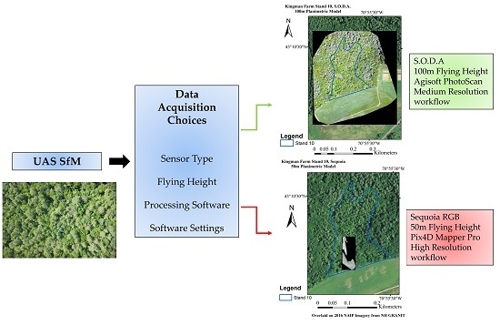
:Unmanned Aerial Systems (UAS) offer users the ability to capture large amounts of imagery at unprecedented spatial resolutions due to their flexible designs, low costs, automated workflows, and minimal technical knowledge barriers. Their rapid extension into new disciplines promotes the necessity to question and understand the implications of data capture and processing parameter decisions on the respective output completeness. This research provides a culmination of quantitative insight using an eBee Plus, fixed-wing UAS for collecting robust data on complex forest environments. These analyses differentiate from measures of accuracy, which were derived from positional comparison to other data sources, to instead guide applications of comprehensive coverage. Our results demonstrated the impacts of flying height on Structure from Motion (SfM) processing completeness, discrepancies in outputs based on software package choice, and the effects caused by processing parameter settings. For flying heights of 50 m, 100 m, and 120 m above the forest canopy, key quality indicators within the software demonstrated the superior performance of the 100-m flying height. These indicators included, among others, image alignment success, the average number of tie points per image, and planimetric model ground sampling distance. We also compared the output results of two leading SfM software packages: Agisoft PhotoScan and Pix4D Mapper Pro. Agisoft PhotoScan maintained an 11.8% greater image alignment success and a 9.91% finer planimetric model resolution. Lastly, we compared the “high” and “medium” resolution processing workflows in Agisoft PhotoScan. The high-resolution processing setting achieved a 371% increase in point cloud density, with a 3.1% coarser planimetric model resolution, over a considerably longer processing time. As UAS continue to expand their sphere of influence and develop technologically, best-use practices based on aerial photogrammetry principles must remain apparent to achieve optimal results.
1. Introduction
Natural systems around the world are experiencing staggering rates of degradation in modern times. Trends in global biodiversity and biogeochemistry have been dominated by human-caused patterns of disturbance [1,2]. Human-led disturbance also alters ecosystem resilience, a long-term feedback generating irrevocable change [3]. Such impacts leave even complex communities functionally extinct, unable to perform their most basic processes. By 2100, the increasing intensity of land-use change is expected to have the most significant impact on biodiversity, influencing key earth system functionality [3,4,5]. The associated interactions of ecosystem and biodiversity change represent a pivotal challenge for ecologists. This complex framework combines the efforts of sustainability, ethics, and policy [2] to manage the future of natural resources.
Forests provide a unique array of ecosystem services to human society, yet still rank among the most exploited of natural environments. The United Nations Food and Agriculture Administration (FAO) estimated that between 2000–2005, forested lands experienced a net global loss of 7.3 million hectares per year [1]. In a more recent 2015 assessment, FAO has estimated a total of 129 million ha of forest land-cover loss between 1990–2015 [6]. This unprecedented level of deforestation elicited action from numerous scientific disciplines, international economies, and facets of government. Similar to many forests around the world, coastal New Hampshire forests have been markedly impacted by disturbance regimes. Local ecosystem services such as nutrient cycling, habitat provisioning, resource allocation, and water quality regulation, which are directly linked to general welfare [7], are experiencing diminished capabilities due to the loss of critical area [8,9]. Many scientific disciplines look to mitigate these impacts and conserve remaining resources but require every advantage of novel strategies and adaptive management to overcome the intricate challenges at hand. To form a comprehensive understanding of natural environments and their patterns of change, scientists and landscape managers must use modern tools to assimilate mass amounts of heterogeneous data at multiple scales. Then, they must translate that data into useful decision-making information [10,11].
Capturing large amounts of data to evaluate the status and impacts of disturbance on the biological composition and structure of complex environments is inherently difficult. The continual change of landscapes, as evident in forest stands in the Northeastern United States [12], further aggravates these intentions. Stimulating conservation science and informing management decisions justifies collecting greater quantities of data and at an applicable accuracy [13,14]. Remote sensing can both develop and enrich datasets in such a manner as to meet the project-specific needs of the end user [15,16]. Remote sensing is experiencing continual technological evolution and embracement to meet the needs of analyzing complex systems [17,18]. This highly versatile tool goes beyond in situ observations, encompassing our ability to learn about an object or phenomenon through a sensor without coming into direct contact with it [19,20]. Most notably, recent advances have enabled data capture at resolutions matching new ranges of ecological processes [18], filling gaps left by field-based sampling for urgently needed surveying on anthropogenic changes in the environment [10,21].
New photogrammetric modeling techniques are harnessing high-resolution remote sensing imagery for unprecedented end-user products with minimal technical understanding [22,23]. Creating three-dimensional (3D) point clouds and planimetric models through Structure from Motion (SfM) utilizes optical imagery and the heavy redundancy of image tie points (image features) for a low-cost, highly capable output [24,25,26,27,28,29,30,31,32]. Although the creation of orthographic and geometrically corrected (planimetric) surfaces using photogrammetry has been around for over 50 years now [33,34], computer vision has only recently linked the SfM workflow to include multi-view stereo (MVS) and bundle adjustment algorithms. This coupled processing simultaneously corrects for parameters and provides an automated workflow for on-demand products [23,35].
As remote sensing continues to advance into the 21st century, new sensors and sensor platforms are broadening the scales at which spatial data are collected. Unmanned Aerial Systems (UAS) is one such platform, being technically defined only by its lack of on-board operator [36,37]. This unrestricted definition serves to exemplify the ubiquitous nature of the tool. Every day there is a wider variety of modifications and adaptations, blurring the lines of classification. Designations such as unmanned aircraft systems (UAS), unmanned aerial vehicles (UAV), unmanned aircrafts (UA), remotely piloted aircrafts (RPA), remotely operated aircrafts (ROA), aerial robotics, and drones all derive from unique social and scientific perspectives [37,38,39,40]. The specification of these titles comes from the respective understanding of the user and their introduction to the platform. Here, UAS is the preferred term due to the platform’s system of components that coordinates the overall operation.
Following a parallel history of development with manned aviation, UAS have emerged from their mechanical contraption prototypes [41] to the forefront of remote sensing technologies [36,39]. Although many varieties of UAS exist today, the majority utilizes some form of: (i) a launch and recovery system or flight mechanism, (ii) a sensor payload, (iii) a communication data link, (iv) the unmanned aircraft, (v) a command and control element, and (vi) most importantly, the human [38,39,40,41,42,43,44].
A more meaningful classification of a UAS may be whether it is a rotary-winged, fixed-winged, or hybrid aircraft. Each aircraft provides unique benefits and limitations corresponding to the structure of its core components. Rotary-winged UAS, which are designated for their horizontally rotating propellers, are regarded for their added maneuverability and hovering capabilities, and for their vertical take-off and landing (VTOL) operation [41]. These platforms are subsequently hindered by their shorter duration flight capacity on average [39]. Fixed-wing UAS, which have been sought after for their longer duration flights and higher altitude thresholds, suffer from a trade-off of focused, extensive coverage. Hybrid unmanned aircraft are beginning to provide realistic utility by combining the advantages of each system including VTOL maneuverability and fixed-wing aircraft flight durations [45]. Each of the systems, with its consumer desired versatility, have driven configurations to meet project needs. Applications such as precision agricultural monitoring [46,47], coastal area management [48], forest inventory [49], structure characterization [50,51], and fire mapping [52] are only a small portion of the fields already employing the potential of UAS [38,40,44,53]. New data products, with the support of specialized or repurposed software functionality, are changing the ways that we model the world. The proliferation of UAS photogrammetry is now recognized by interested parties in fields such as computer science, robotics, artificial intelligence, general photogrammetry, and remote sensing [23,40,43,54].
The rapid adoption of this new technology brings cause for questions as to how it will inevitably affect other, more intensive aspects of society. Major challenges to the advancement of UAS include understandings of privacy, security, safety, and social concerns [40,44,55]. These major influences are causing noticeable shifts in the worldwide acceptance of the platform, and spurring regulations as outcomes of the conflict of interest between government and culture [39,53,54,56]. In an initiative to more favorably integrate UAS into the National Airspace System (NAS) of the United States (US), the Federal Aviation Administration (FAA) established the Remote Pilot in Command (RPIC) license under 14 Code of Federal Regulations (CFR) [57]. RPIC grants permission for low-altitude flights, under restricted flexibility, to overseers with sufficient aeronautical knowledge [58].
Evidence of the shift towards on-demand spatial data products is everywhere [44,59]. The extremely high resolution, flexible operation, minimal cost, and automated workflow associated with UAS make them an ideal remote sensing platform for many projects [43,53,59,60]. However, as these systems become more integrated, it is important that we remain cognizant of factors that may affect data quality and best-use practices [23]. Researchers in several disciplines have investigated conditions for data capture and processing that may decrease positional certainty or reliability [38]. These studies provide comparative analysis of the UAS-SfM data products to highly precise sensors such as terrestrial laser scanners (TLS), light detection and ranging (LiDAR) systems, and ground control point surveying [30,32,35,49,51,61]. However, fewer studies and guidelines have provided clear quantitative evidence for issues affecting the comprehensive coverage of study sites using UAS-SfM, especially for complex natural environments [62,63]. The principles expressed here reflect situations in which the positional reliability of the resulting products is not the emphasis of the analysis. Instead, our research provides an overview of the issues associated with the use of UAS for data collection and processing to capture complex forest environments in an effective manner. Specifically, our objectives were to: (i) analyze the effects of image capture height on SfM processing success, and (ii) determine the influences of processing characteristics on output conditions by applying multiple software packages and workflow settings for modeling complex forested landscapes.
2. Materials and Methods
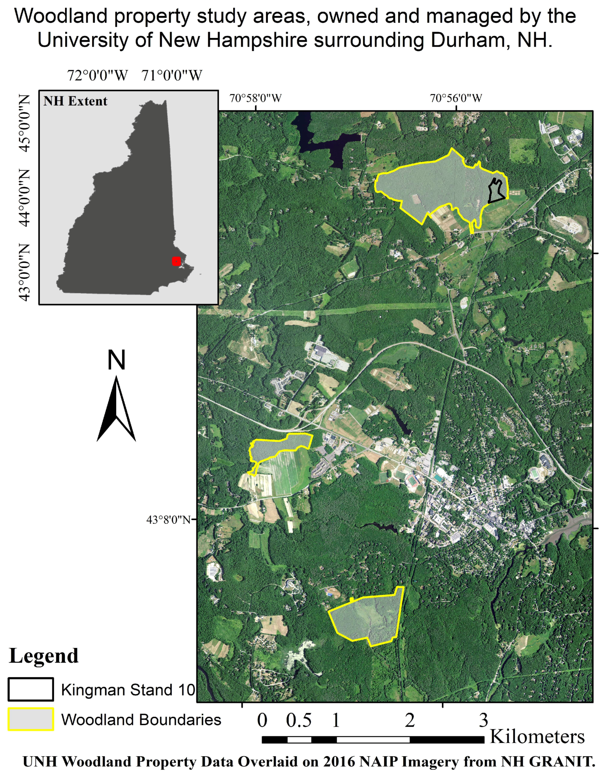
This research was conducted using three woodland properties owned and managed by the University of New Hampshire, Durham, New Hampshire, USA. These properties included Kingman Farm, Moore Field, and West Foss Farm, totaling approximately 154.6 ha of forested land (235.2 ha of total area), and were located in the seacoast region of New Hampshire (Figure 1). Our research team was granted UAS operational permission to fly over each of these forested areas, which were selected for their similarity to the broader New England landscape mosaic [64]. For our first objective, the analysis of flying height on image processing capabilities, a sub-region of Kingman Farm designated as forest stand 10 [65] was selected. Stand 10, comprising 3.6 ha (.036 km2) of red maple swamp and coniferous patches, was used due to its overstory diversity and proximity to an open ground station area. Part of the second objective—establishing a comparison between software packages for forest landscape modeling—required a larger area of analysis. For this reason, processed imagery across all three woodland properties—Kingman Farm (135.17 ha), West Foss Farm (52.27 ha), and Moore Field (47.76 ha)—was used. The other part of the second objective, determining the influences on processing workflow settings on the SfM outputs, utilized the Moore Field woodland property as an exemplary subset of the regional landscape.
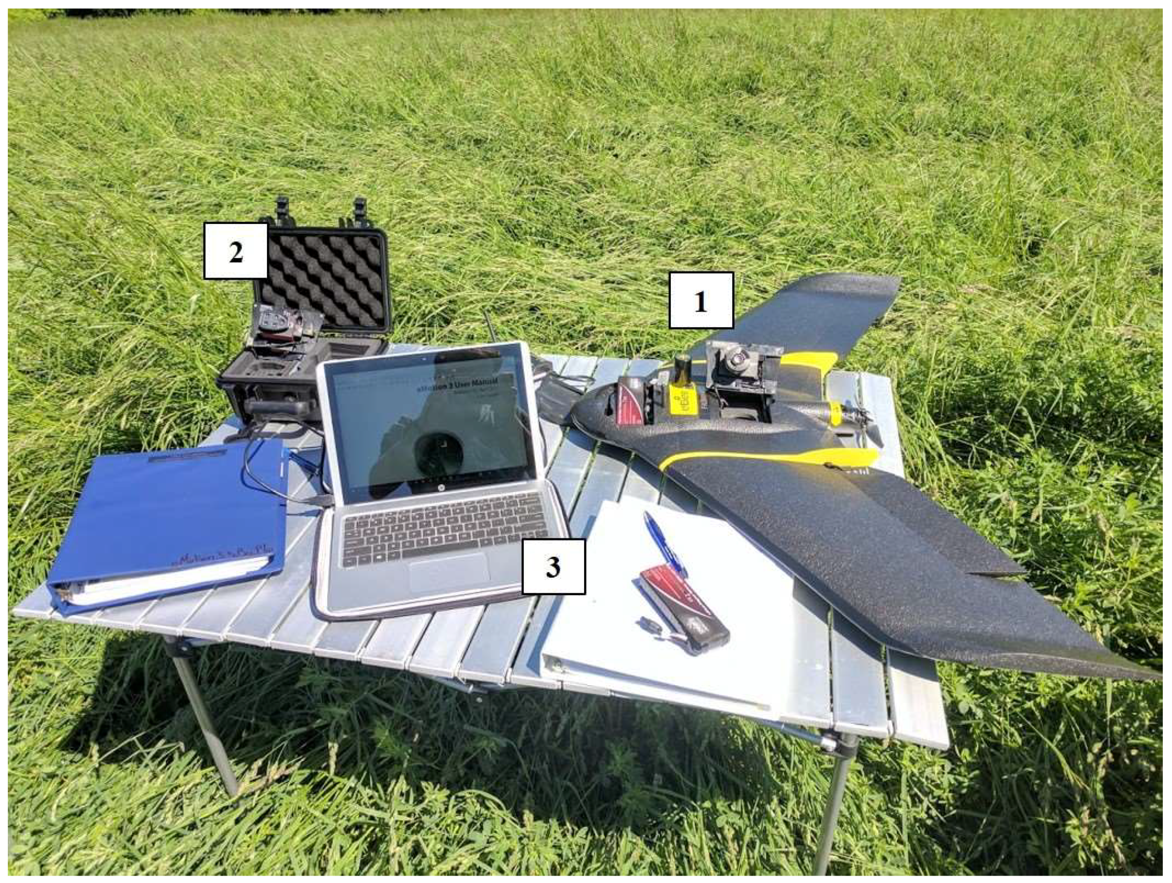
A SenseFly eBee Plus by Parrot, Cheseaux-sur-Lausanne, Switzerland, (Figure 2) was used to evaluate the utility of fixed wing UAS. With integrated, autonomous flight controller software (eMotion 3 version 3.2.4, senseFly Parrot Group, Cheseaux-sur-Lausanne, Switzerland), a communication data link, and an inertial measurement unit (IMU), this platform boasted an expected 59 min flight time using one of two sensor payloads. First, the Sensor Optimized for Drone Applications (S.O.D.A) captured 20 MP of natural color imagery. Alternatively, the Parrot Sequoia sensor incorporated five optics into a multispectral system, including a normal color 16 MP optic and individual blue, green, red, red edge, and near infrared sensors. For our purposes, we solely compared the Sequoia RGB sensor to the S.O.D.A. For the rest of this analysis, we will refer to this single sensor.
To alleviate climatic factors influencing image capture operations, cloudy weather and near dawn or dusk flights were avoided in lieu of optimal sun-angle and image consistency [62]. Prior day weather forecasting from the National Weather Service (NWS) and drone-specific flight mapping services was checked. Maintaining image capture spacing regularity during flight planning is also heavily influential on processing effectiveness. Therefore, wind speeds in excess of 12 m/s were avoided, despite the UAS being capable of operating in speeds up to 20 m/s. In addition, flight lines were oriented perpendicular to the prevailing wind direction. These subtle operational considerations, while not particularly noticeable in the raw imagery, are known to improve overall data quality [62,63] and mission safety.
To analyze the efficiency and effectiveness of the UAS image collection process, several flying heights and two sensor systems were compared. These flying heights were determined using a canopy height model provided through a statewide LiDAR (.las) dataset [66]. The LiDAR dataset was collected between the winter of 2010 and the spring of 2011 under a United States Geological Survey (USGS) North East Mapping project [67]. The original dataset was sampled at a two-meter nominal scale, and was upscaled to a 10-meter nominal scale using the new cells maximum value. Then, it was cleaned so as to both provide the UAS with a more consistent flight altitude, and ensure safety from structure collisions. Setting the flying height above the canopy height model more importantly ensured that images kept a constant ground sampling distance (gsd), or model pixel size, during processing. It was originally intended to evaluate flying heights of 25 m, 50 m, and 100 m above this canopy height model. However, test missions proved that flying below 50 m quickly lost line-of-sight (a legal requirement) and the communication link with the ground control station. With the goal of determining the optimal height for: high spatial resolution, processing efficiency, and maintaining a safe operation, flying heights of 50 m, 100 m, and 120 m above the forest canopy were selected. Since these flying heights focus on the forest canopy layer, and not the ground, all of the methods and results are set relative to this height model. These flying heights represented a broad difference in survey time of approximately 9 min to 18 min per mission for the given study area, stand 10, and an even greater difference in the number of images acquired (337 at 50 m with the S.O.D.A, and 126 at 120 m). The threshold of 120 m was based on CFR 14 Part 107 restrictions, stating all UAS flights are limited to a 400 ft above-surface ceiling [58]. Additional flying heights at lower altitudes have been tested for rotary-winged UAS [60,62].
Similar to the traditional photogrammetric processes of transcribing photographic details to planimetric maps using successive image overlap [68], successful SfM modeling from UAS collected imagery requires diligent consideration of fundamental flight planning characteristics. Generating planimetric models, or other spatial data products from UAS imagery, warrants at least a 65% end (forward) and sidelap based on user-recommended sampling designs [69]. The computer vision algorithms rely on this increased redundancy for isolating specific tie points among the high levels of detail and inherent scene distortions [27,30,32]. Many practitioners choose even higher levels of overlap to support their needs for data accuracy, precision, and completeness. For complex environments, recommended image overlap increases to 85% endlap and 70% to 80% sidelap [70]. For all of the missions, we applied 85% endlap and 70% sidelap, which approached the maximum possible for this sensor.
The first step in processing the UAS images captured by the S.O.D.A and Sequoia red–green–blue (RGB) sensors was to link their spatial data to the raw imagery. Image-capture orientation and positioning was collected by the onboard IMU and global positioning system (GPS) and stored in the flight log file (.bbx). A post-flight mission planning process imbedded in the eMotion3 flight planning software accessed the precise timing of each camera trigger in the flight log automatically when connected to the eBee Plus and automated the spatial matching process.
All of the processing was performed on the same workstation, a Dell Precision Tower 7910 with an Intel Xenon E5-2697 18 core CPU, 64GB of RAM, and a NIVIDIA Quadro M4000 graphics card. The workflows in both software packages created dense point clouds using MVS algorithms a 3D surface mesh, and a planimetric model (i.e., orthomosaic) using their respective parameters. In Pix4D Mapper Pro (Pix4D), Lausanne, Switzerland, when comparing the impact of flying height against processing effectiveness as part of our first objective, several processing parameters were adjusted to mitigate the complications for computer vision in processing the forest landscape. All of the combinations of sensor and flying height SfM models used a 0.5 tie-point image scale, a minimum of three tie points per processed image, a 0.25 image scale with multi-scale view for the point cloud densification, and triangulation algorithms for generating digital surface models (DSM) from the dense point clouds [70]. The tie-point image scale metric reduced the imagery to half its original size (resolution) to reduce the scene complexity while extracting visual information [69]. We used a 0.25 image scale while generating the dense point cloud to further simplify the raw image geometry for computing 3D coordinates [70]. Although these settings promote automated processing speed and completeness in complex landscapes, their use could influence result accuracy and should be used cautiously.
For both objectives, we used key “quality” indicators within the software packages to assess SfM model effectiveness. First, image alignment (“calibration” in the software) denotes the ability to define the camera position and orientation within a single block, using identified tie point coordinates [22,27,71]. Manual tie point selection using ground control points or other surveyed features was not used to enhance this. Only images that were successfully aligned could be used for further processing. Camera optimization determined the difference between the initial camera properties and the transformed properties generated by the modeling procedure [71]. The average number of tie points per image demonstrated how much visual data could be automatically generated. The average number of matches per image showed the strength of the tie-point matching algorithms between overlapping images. The mean re-projection error calculated the positional difference between the initial and final tie-point projection. Final planimetric model ground sampling distances (cm/pixel) and their surface areas were observed to assess the completeness and success of the procedure. Lastly, we recorded the total time required for processing each model.
Another key consideration of SfM processing was the choice of software package used in the analysis. As part of the second objective, we investigated the influence of the software package choice on model completion. Leading proprietary UAS photogrammetry and modeling software packages Agisoft PhotoScan (Agisoft) and Pix4D have garnered widespread adoption [23,38,49,72,73]. The initial questioning of other users (ASPRS Conference in spring 2016) and test mission outputs provided inconsistent performance reviews to judge a superior workflow. Although open source UAS-SfM software has become increasingly accessible and renowned, only these software came recommended as total solutions for our hardware and environment. To contrast the two packages in their ability to model the forest landscape, all three woodland properties were processed and analyzed. To remain consistent between Agisoft and Pix4D workflow settings, we used “High” or “Aggressive” (depending on software vocabulary) image alignment accuracy, 0.5 tie-point image scales, and a medium resolution mesh procedure.
To accomplish our final objective and evaluate the capabilities of the suggested default resolution processing parameters further, Moore Field was processed individually using both medium and high-resolution (“quality”) settings within Agisoft. During this final analysis, we adjusted only the model resolution setting during the batch processing between each test, and again used the 0.5 tie-point image scale for both. The outputs were compared based on the image alignment success, the total number of tie points formed, the point cloud density, and the planimetric model resolution.
3. Results
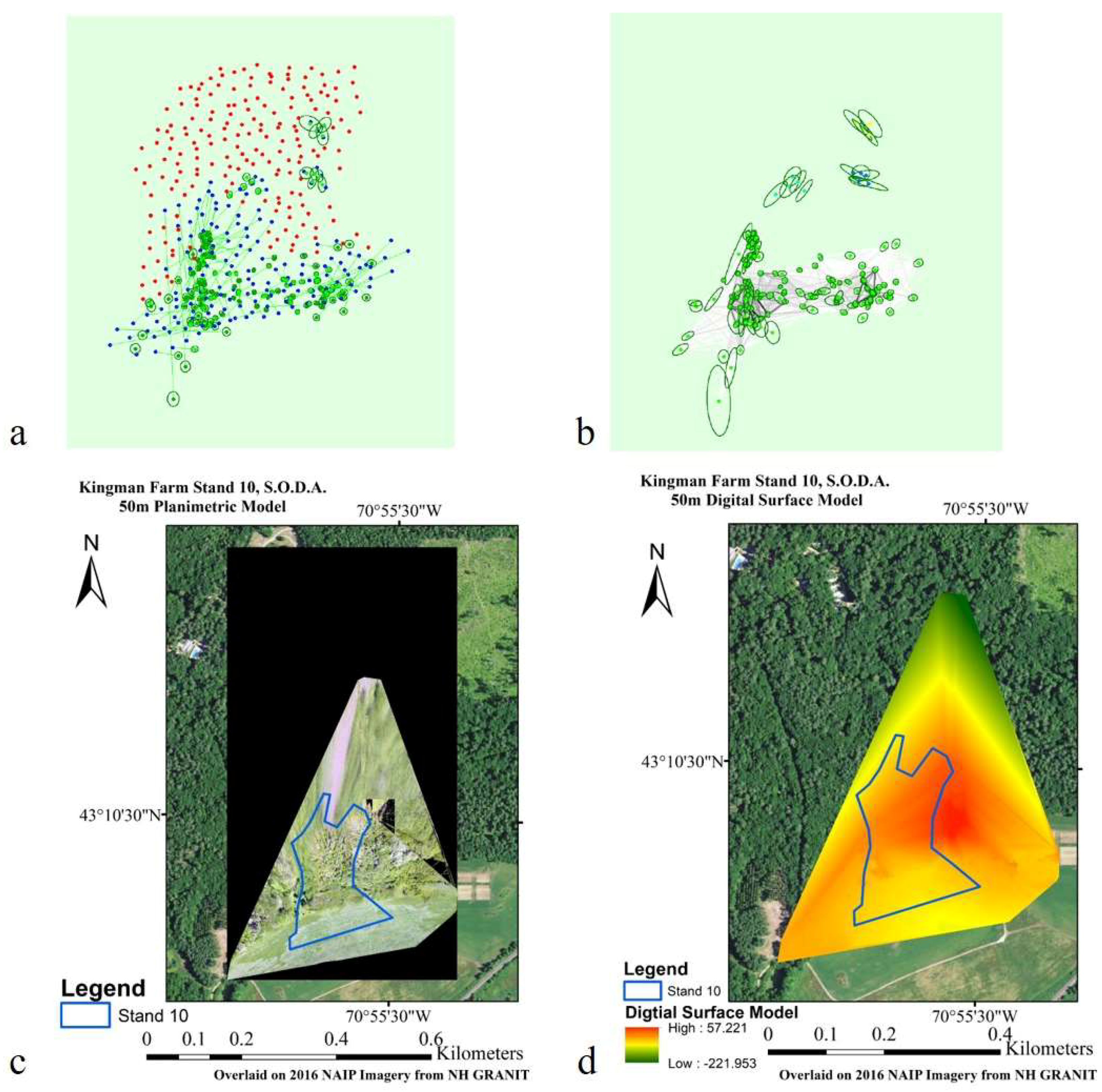
The results of the data processing for UAS imagery collected 50 m, 100 m, and 120 m above complex forest community canopies demonstrated significant implications regarding the effectiveness of the data collection. At 50 m above the forest canopy the S.O.D.A. sensor collected 337 images covering Stand 10 of Kingman farm. Using the Pix4D software to process the imagery, 155 out of the 337 (45%) of the images were successfully aligned for processing to at least three matches (Figure 3a), with a 5.53% difference in camera optimization. The processing took a total of 69:06 min, in which an average of 29,064 image tie points and 1484 tie-point matches were found per image. The distribution of tie point matches for each aligned image can be seen in Figure 3b, with a gradient scale representing the density of matching. Additionally, geolocation error or uncertainty is shown for each image with its surrounding circle size. The final planimetric model covered 30.697 ha (0.307 km2) with a 3.54-cm gsd (Figure 3c), and a 0.255 pixel mean re-projection error. Successful image alignment and tie-point matching were limited to localized regions near the edges of the forested area to the south, promoting significant surface gaps and extrapolation within the resulting DSM and planimetric model (Figure 3c,d).
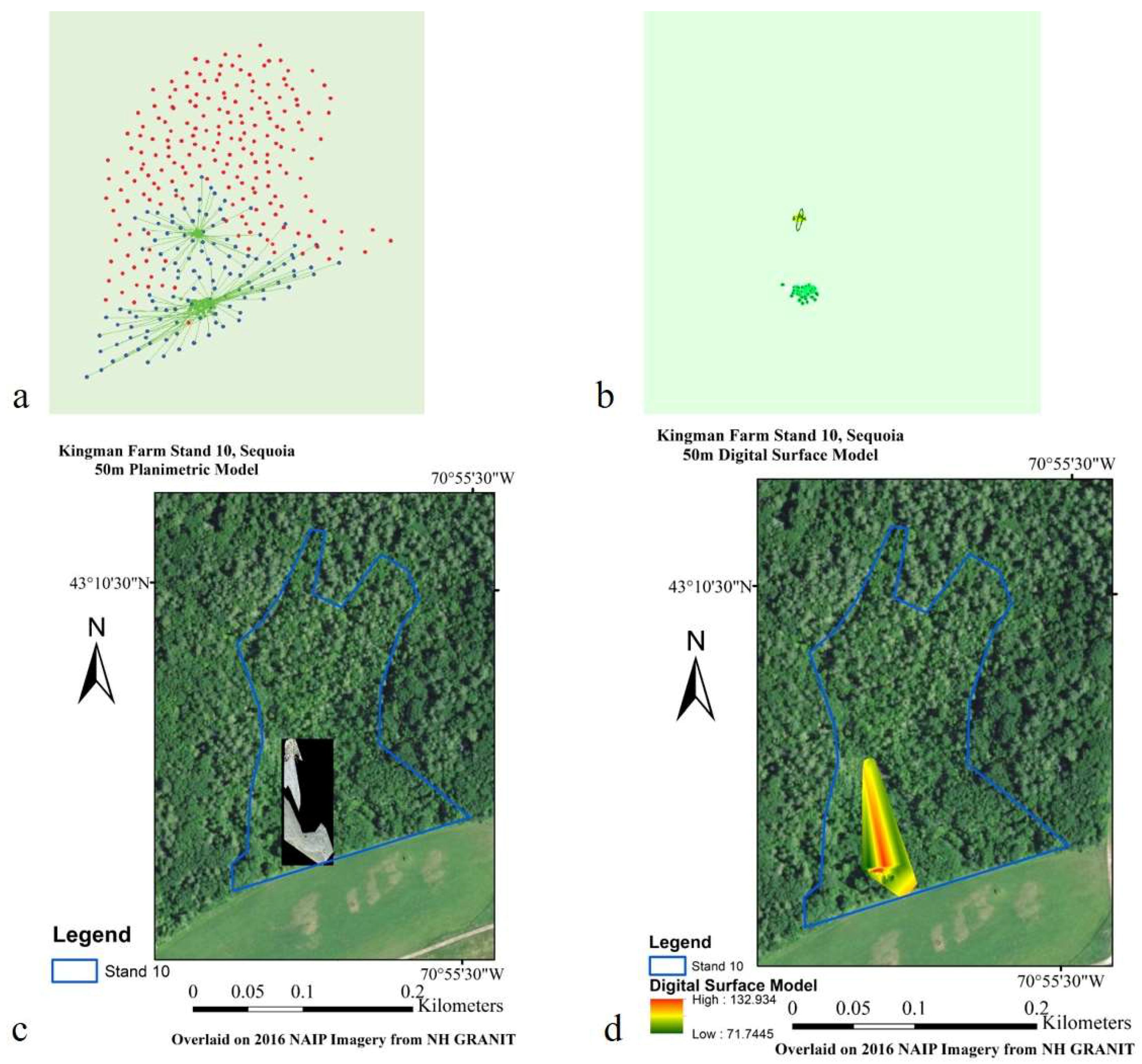
Capturing imagery with the Sequoia RGB multispectral sensor at a height of 50 m above the canopy produced 322 images, of which 122 (37%) could be aligned successfully (Figure 4a). The majority of which were again localized to the southern, forest edge. The overall camera optimization difference was 1.4%. The average number of image tie points and tie-point matches were 25,561 and 383.91 per image, respectively. However, all of these tie point matches appeared to be concentrated on a small area within the study site (Figure 4b). This processing workflow, lasting 43:21 min, created a final orthomosaic covering 0.2089 ha (0.0021 km2) at a 0.64-cm gsd, and a 0.245 pixel mean re-projection error (Figure 4c). Image stitching for this flight procedure recognized image objects in only two distinct locations throughout the study area, forcing widespread irregularity for the minimal area that was produced (Figure 4a–d).
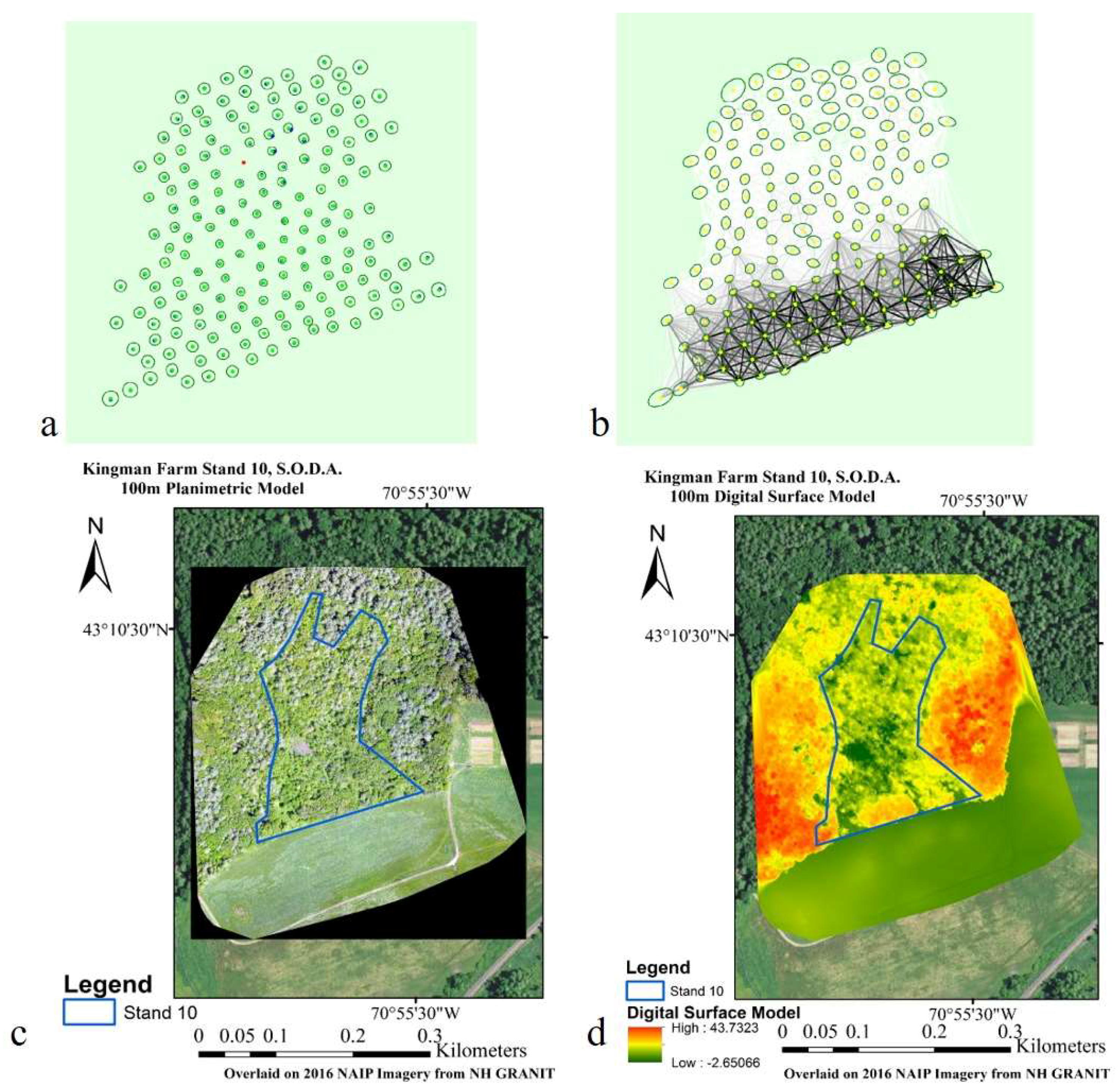
Beginning at 100 m above the forest canopy, UAS-SfM models more comprehensively recognized the complexity of the forest vegetation. At 100 m, with the S.O.D.A. sensor, data processing aligned 176 of 177 (99%) of the collected images at a 0.45% camera optimization difference (Figure 5a). Pix4D generated an average of 29,652 image tie points with 2994.12 tie-point matches per image. The distribution and density of tie point matching (Figure 5b) between overlapping images can be seen to more thoroughly cover the entire study area. Finishing in 84:15 min, the final planimetric output had a 3.23-cm gsd, covered 16.5685 ha (0.1657 km2), and had a mean re-projection error of 0.140 (Figure 5c). Camera alignment, image tie-point matching, and planimetric processing results portrayed greater computer recognition and performance with minimal incomprehension near the center of the forest stand (Figure 5). The DSM for this flying height and sensor show far greater retention of the forest stand (Figure 5d).
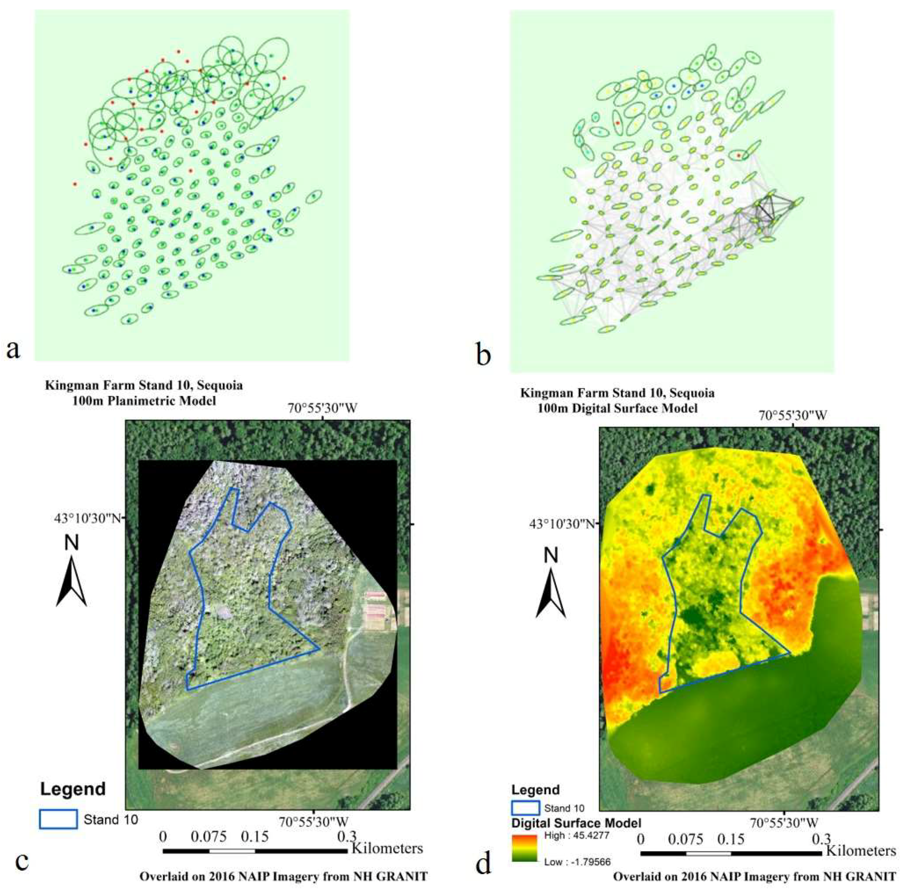
Alternatively, the Sequoia RGB sensor at 100 m above the canopy successfully aligned 159 of 178 (89%) collected images. The failure of the remaining images in the northern part of the study area (Figure 6a) corresponded with a considerably greater number of image geolocation errors and tie-point matches (Figure 6b). This workflow took the greatest amount of processing time of 133:08 min, with 25,825 image tie points and 902.51 tie-point matches on average. The camera optimization difference with this height and sensor combination was 0.87%. The planimetric model covered 14.32 ha (0.1432 km2), had a 3.95-cm gsd, and a mean re-projection error of 0.266 pixels (Figure 6c). Both the planimetric model (Figure 6c) and DSM (Figure 6d) covered the entirety of the study area, with diminished clarity along the northern boundary.
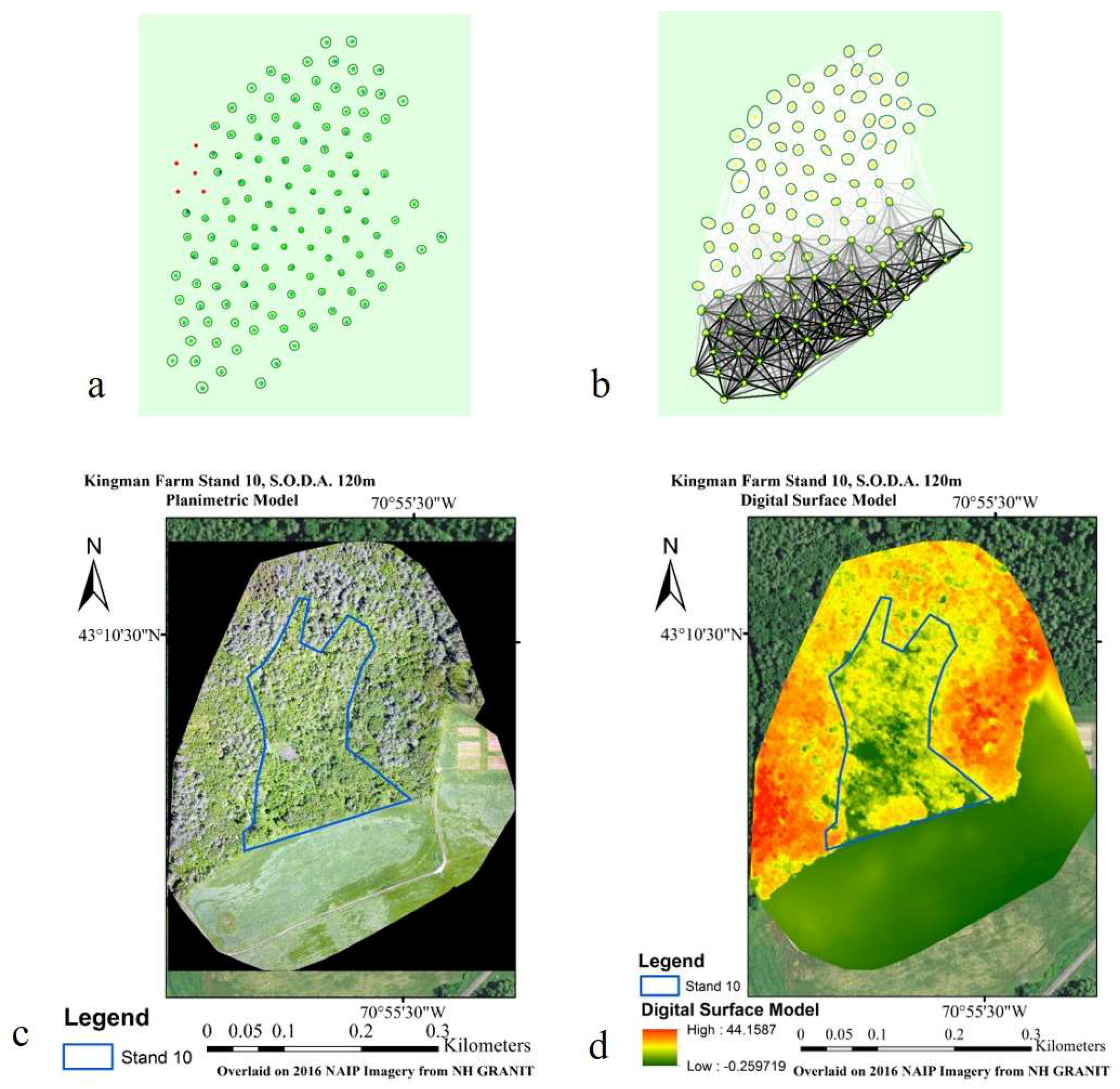
At the highest flying height, 120 m above the canopy surface, processing of the S.O.D.A. imagery successfully aligned 121 of 126 (96%) images with a 0.44% camera optimization difference. The five images that could not be represented were clumped near the northwestern corner of the flight plan (Figure 7a). Images averaged 29,168 tie points and 3622.33 tie-point matches. The distribution of tie-point matches (Figure 7b) showed moderate density throughout the study area, with greatest connectivity along the southern boundary (Figure 7b). After 52:32 min of processing, an 18.37-ha (0.1837 km2) planimetric surface was generated with a 3.8-cm gsd and a 0.132 pixel re-projection error Figure 7c). The resulting DSM (Figure 7d) and planimetric model were created with high image geolocation precision and image object matching across the imagery (Figure 7). The entirety of the study area for this model is visually complete.
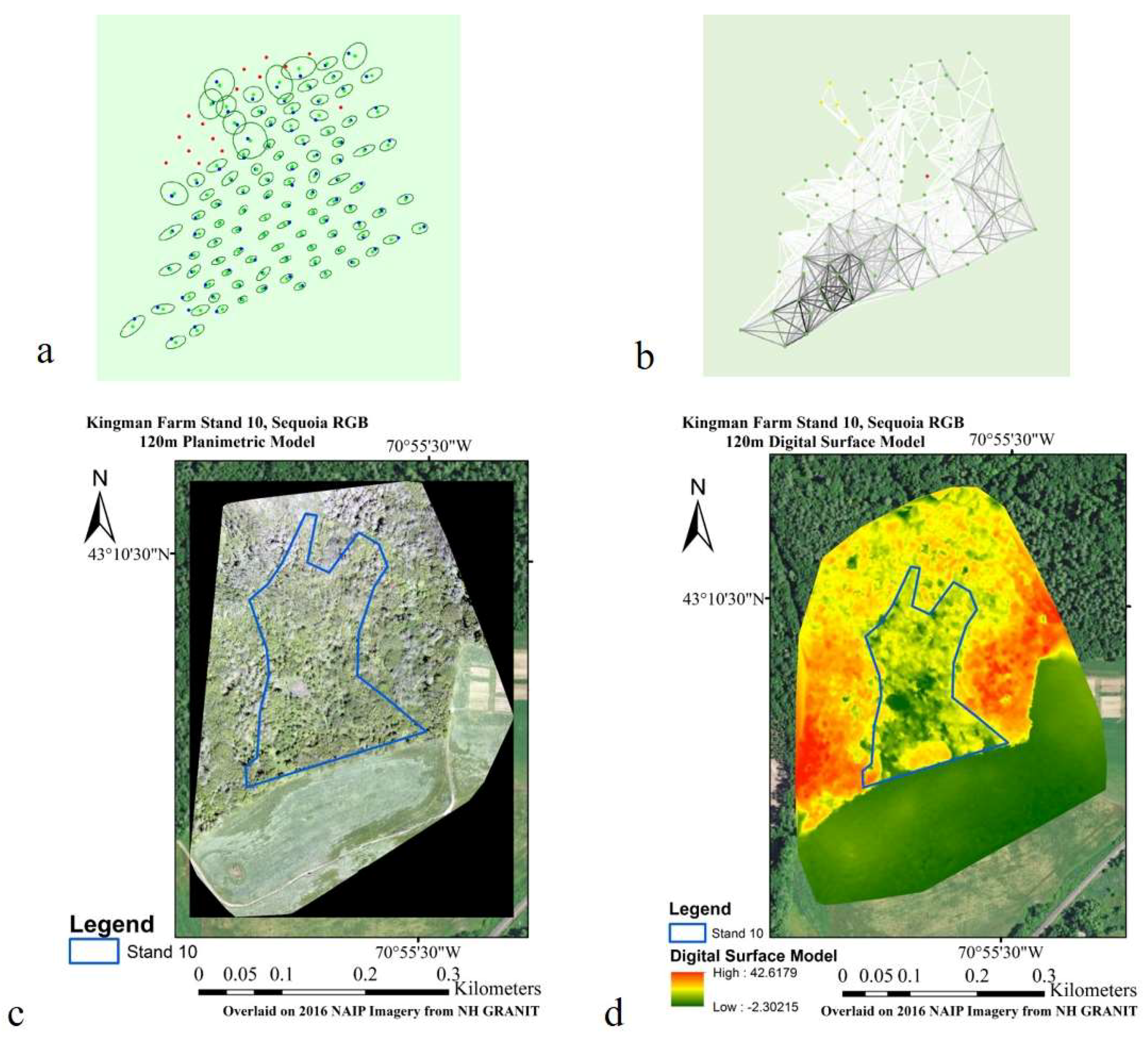
Finally, the Sequoia RGB sensor flying at 120 m above the forest canopy captured 117 images, of which 102 (87%) were aligned. The image alignment and key point matching diagrams (Figure 8a,b) showed lower comprehension throughout the northern half of the study area, corresponding with the interior forest. Pix4D processing resulted in a 1.73% camera optimization difference with an average of 25,505 tie points and 1033.83 tie point matches per image. The overall processing time was 50:13 min, which generated a 14.926 ha (0.1493 km2) planimetric model at a 4.44 cm-gsd and 0.273 pixel re-projection error (Figure 8c). Weak image alignment and tie-point matching in the upper half of the forest stand formed regions of inconsistent clarity along the edges of the study area (Figure 8c,d).
In summary, Table 1 shows an evaluation of the results from the six sensor and flying height combinations utilized by the eBee plus UAS. The degree of processing completeness is shown to be heavily influenced by UAS flying height, as demonstrated by variables such as image alignment success, camera optimization, average tie-point matches per image, and the area covered by the models. Flying heights of 100 m and 120 m above the forest canopy both display greater image alignment and tie-point matching success than the 50-m flying height. Although the 50-m flying height did have a slightly finer overall ground sampling distance and re-projection error, these results should be understood in the broader context of the resulting SfM data products. The 100-m flying height demonstrated the most comprehensive alignment of images for both sensors. This increase in image alignment success and average tie points per image also came with a noticeably longer processing duration. However, when comparing image re-projection error and average matching per image indicators for the 100-m and 120-m flying heights, the 120-m model processing contained less uncertainty (Figure 5 and Figure 7).
Comparing the S.O.D.A. sensor to the Sequoia RGB sensor across the three flying heights resulted in, on average, a 9% greater image alignment success rate, a 14.29% greater number of tie points per image, an increase of 356.21% in image matches, and a 32.3% lower re-projection error for the S.O.D.A. Ground sampling distances for the two sensors were not quantitatively compared because of the inconsistency of the model completion.
Comparison of the processing of all three woodland properties using both Pix4D and Agisoft demonstrated clear differences in results for the same imagery. Across the combined 3716 images (covering 235.2 ha), Agisoft had an 11.883% higher image alignment success. The final planimetric models also had a 9.91% finer resolution (lower gsd) using Agisoft. However, this increase in gsd resulted in 67.3% fewer tie points (Table 2).
Within Agisoft itself, several processing workflow complexities are available. In this analysis, we compared the medium and high-resolution (“quality”) point cloud generation procedures to determine their influence on the final planimetric model outputs. In processing Moore Field, we saw an increase in overall tie points of 31.3% (346,598 versus 264,015), an increase of 371% in photogrammetric point cloud density (187.3 m versus 50.5 m), and a 0.01-cm increase in final ground sampling distance (3.33 cm versus 3.32 cm) when using the high versus medium settings (Table 3). However, the difference in processing time for the higher resolution model was in the order of days.
4. Discussion
The effects of flying height on SfM processing capability, as shown in Table 1, demonstrate a clear influence on output completeness. All of the three analyses offered insight into complications for obtaining visually complete complex forest models. These study areas presented forests with closed, dense canopies comprising a great deal of structural and compositional diversity, which are typical of the New England region. These forests represent some of the most complex in the world although they are less complex than tropical rain forests. Issues discussed here are appropriately applied to forests of similar complexity. In simpler forest environments with less species diversity and more open canopies, the issues discussed here will be less problematic. In these New England forests, the complexity of the imagery at such a fine scale leads to difficulties in isolating tie points [74]; these difficulties were exacerbated at the 50-m flying height. Compounding disruptions of the fixed flight speed, sensor settings, and flight variability further biased this flying height. Image alignment and tie-point generation with either the S.O.D.A or the Sequoia RGB sensor at this low altitude was inconsistent and error-prone (Figure 3 and Figure 4). This lack of comprehension for initial processing reverberated heavily in the DSMs and planimetric models, generating surfaces largely through extrapolation. Flying at 100 m and 120 m above the forest canopy, image alignment success ranged from 89–99% with ground sampling distances of 3.23–3.8 cm for the S.O.D.A and 3.95–4.44 cm for the Sequoia RGB sensor. These increases in successful image and scene processing were accompanied by a much larger number of average tie-point matches per image. For both sensors, the 100-m flying height appeared to out-compete even that of 120 m, with a higher resolution and image calibration success. The resulting slight difference in GSD for the two flying heights was likely a function of the variation in flight characteristics for the aircraft during image capture, leading to deviations in camera positions, and averaged point cloud comprehension for the forest canopy. Looking at the image tie-point models (Figure 7 and Figure 8) shows that this remaining uncertainty or confusion is clustered in the upper corner of the study area, corresponding with the mission start. Several factors could have influenced this outcome, with the most direct impact suggesting environmental stochasticity (i.e., short-term randomness imposed within the environment); for example, canopy movement or the sun angle diminishing tie-point isolation [62,63,75]. Other possibilities for the clustered uncertainty include UAS flight adjustments during camera triggering, leading to discrepancies in the realized overlap, and image motion blur.
Understandably, the Sequoia RGB sensor achieved less comprehensive results compared with the S.O.D.A., which has a sensor that is more specifically designed for photogrammetric modeling. When comparing average results across the 50-m, 100-m, and 120-m flying heights, the Sequoia accomplished 9% lower image alignment success, 14.29% fewer tie points, 356% fewer matches, and a 32.3% higher re-projection error (Table 1). The processed models became rampant with artifacts and areas void of representation because of a combination of dense vegetation causing scene complexity and camera characteristic differences. Recommended operations for the Sequoia sensor include lowering the flight speed (not capable on the eBee Plus) and increasing flying height to overcome its rolling shutter mechanics, which negatively impact image geolocation (Figure 4a,b). The creation and deployment of optimized sensors for UAS (i.e., the S.O.D.A. sensor) is a simple yet direct demonstration of increased efficiency and effectiveness behind this rapidly advancing technology and the consumer demand supporting it.
Given the unresolved processing performance for complex natural environments, our study also investigated whether Agisoft or Pix4D generated higher quality SfM outputs. With 11.8% greater image alignment and 9.9% finer resolution, Agisoft appeared to have an advantage (Table 2). However, determining any universal superiority proved difficult due to the “black box” processing imposed at several steps in either software package [23,27]. Pix4D maintained 67.3% more tie points across the three study areas and provided a more balanced user interface, including adding in a variety of additional image alignment parameters and statistical outputs. Pix4D can be more favorable to some users because of its added functionality and statistical output transparency, including: added task recognition during processing, an initial quality report, a tie-point positioning diagram, geolocation error reporting, image-matching strength calculations, and a processing option summary table. However, for the final planimetric model production, Agisoft performed to a superior degree based on SfM output completeness and visualization indicators.
Lastly, we contrasted the medium and high-resolution workflows in Agisoft to determine the impact on modeling forest landscapes. The high-resolution processing workflow experienced a 371% increase in point cloud density. However, the final planimetric models were only marginally impacted at 3.33 cm and 3.32 cm for high and medium-resolution processing, respectively (Table 3). The slightly improved results were not worth the extra processing time, as the high-resolution workflow took days rather than hours to complete. UAS are sought after for their on-demand data products, further legitimizing this preference [25,38,43]. Assessing the represented software indicators demonstrated that the sensor, software package, and processing setting choice did each affect UAS-SfM output completeness, implying a need to balance output resolution and UAS-SfM comprehension. For our study area, this supported using the S.O.D.A. at a 100-m flying height above the canopy, with a medium-resolution processing workflow in Agisoft PhotoScan. It should be remembered that these conclusions are relative to the forest canopy, as well as our objective for modeling the landscape. These results and software indicators should be considered carefully when assessing photogrammetric certainty. However, depending on the nature of other projects or their restrictions, alternative combinations of each could be implemented.
Many additional considerations for UAS flight operations could be included within these analyses, especially in light of more traditional aerial photogrammetry approaches. Our analyses specifically investigated the ability of UAS-SfM to capture the visual content of the forested environment, but not its positional reliability. To improve computer vision capabilities, multi-scale imagery could have been collected [49]. Perpendicular flight patterns or repeated passes could have been flown. These suggestions would have increased operational requirements, and thus decreased the efficiency of the data collection. Alternatively, greater flying heights could have been incorporated (e.g., 250 m above the forest canopy). The maximum height used during our research was set by the current FAA guidelines for UAS operations [58]. Future legislation changes or special waivers for flight ceilings should consider testing a wider range of altitudes for both sensors. Despite the recommendation for maintaining at least a 10-cm gsd to adequately capture complex environments [63,69,70], several models created in this research produced comprehensive planimetric surfaces. Producing a 10-cm gsd would also require flying above the legal 121.92 m ceiling under the current FAA regulations.
Unmanned aerial systems have come a long way in their development [39,41], yet still have much more to achieve. The necessity for high-resolution products with an equally appropriate level of completeness is driving hardware and software evolution at astonishing rates. To match the efficiency and effectiveness of this remote sensing tool, intrinsic photogrammetric principles must be recognized. Despite limitations on flight planning [55], and computer vision performance [22,27,76], UAS can produce astounding results.
5. Conclusions
Harnessing the full potential of Unmanned Aerial Systems requires diligent consideration of their underlying principles and limitations. To date, quantitative recognition of their best operational practices are few and far between outside of positional reliability [49,62,77,78]. This is despite their exponentially expanding user base and the increasing reliance on their acquired data sets. In conjunction, SfM data processing has not yet set data quality or evaluation standards [23]. As with any novel technology, these operational challenges and limitations are intrinsic to our ability to acquire and rightfully use such data for decision-making processes [79,80]. The objective of this research was to demonstrate a more formal analysis of the data acquisition and processing characteristics for fixed-wing UAS. The three analyses performed here were a result of numerous training missions, parameter refinements, and knowledge base reviews [69,70], in an effort to optimally utilize UAS-SfM for creating visual models. Our analysis of the effects of flying height on SfM output comprehension indicated an advantage for flying at 100 m above the canopy surface instead of a lower or higher altitude. This is based on a higher image alignment success rate, and a finer resolution orthomosaic product. In comparing Agisoft PhotoScan and Pix4D Mapper Pro software packages across 235.2 ha of forested land, Agisoft generated more complete UAS-SfM outputs. This is the result of greater image alignment success creating a more complete model, as well as a finer resolution output. Lastly, the evaluation of the workflow settings endorsed medium-resolution processing because of a substantial trade-off between point cloud density, 371% difference, and processing time efficiency. Each of these results was found from the mapping of dense and heterogeneous natural forests. Such outputs are important for land management and monitoring operations.
The photogrammetric outputs derived from the UAS-SfM of complex forest environments represent a new standard for remote sensing data sets. To support the widespread consumer adoption of this approachable platform, our research went beyond the often-limited guides on photogrammetric principles and provided quantitative evidence for optimal practices. With the increasing demand for minimizing costs and maximizing output potential, it is still important to thoroughly consider the influence of flight planning and processing characteristics on data quality. The results presented support these interests, allowing for the collection of data for and the SfM processing of visually complete models of complex natural environments. As associated hardware, software, and legislation continue to develop, transparent standards and assessment procedures will benefit all stakeholders enveloped in this exciting frontier.
Author Contributions
B.T.F. and R.G.C. conceived and designed the experiments; B.T.F. performed the experiments and analyzed the data with guidance from R.G.C.; R.G.C. provided the materials and analysis tools; B.T.F. wrote the paper; R.G.C. revised the paper and manuscript.
Funding
This research was partially funded by the New Hampshire Agricultural Experiment Station. The Scientific Contribution Number is 2769. This work was supported by the USDA National Institute of Food and Agriculture McIntire Stennis Project #NH00077-M (Accession #1002519).
Acknowledgments
These analyses utilized processing within Pix4D Mapper Pro and Agisoft Photoscan Software Packages with statistical outputs generated from their results. All UAS operations were conducted on University of New Hampshire woodland properties with permission from local authorities and under the direct supervision of pilots holding Part 107 Remote Pilot in Command licenses.
Conflicts of Interest
The authors declare no conflict of interest.
References
- Kareiva, P.; Marvier, M. Conservation Science: Balancing the Needs of People and Nature, 1st ed.; Roberts and Company Publishing: Greenwood Village, CO, USA, 2011; p. 543. [Google Scholar]
- McGill, B.J.; Dornelas, M.; Gotelli, N.J.; Magurran, A.E. Fifteen forms of biodiversity trend in the Anthropocene. Trends Ecol. Evol. 2015, 30, 104–113. [Google Scholar] [CrossRef] [PubMed]
- Chapin, F.S., III; Zavaleta, E.S.; Eviner, V.T.; Naylor, R.L.; Vitousek, P.M.; Reynolds, H.L.; Hooper, D.U.; Lavorel, S.; Sala, O.E.; Hobbie, S.E.; et al. Consequences of changing biodiversity. Nature 2000, 405, 234. [Google Scholar] [CrossRef] [PubMed]
- Lambin, E.F.; Turner, B.L.; Geist, H.J.; Agbola, S.B.; Angelsen, A.; Bruce, J.W.; Coomes, O.T.; Dirzo, R.; Fischer, G.; Folke, C.; et al. The causes of land-use and land-cover change: Moving beyond the myths. Glob. Environ. Chang. 2001, 11, 261–269. [Google Scholar] [CrossRef]
- Smith, W.B. Forest inventory and analysis: A national inventory and monitoring program. Environ. Pollution 2002, 116, S233–S242. [Google Scholar] [CrossRef]
- Food and Agriculture Organization of the United Nations. Global Forest Resources Assessment 2015. In How Are the World’s Forests Doing? 2nd ed.; FAO: Rome, Italy, 2016; pp. 2–7. [Google Scholar]
- MacLean, M.G.; Campbell, M.J.; Maynard, D.S.; Ducey, M.J.; Congalton, R.G. Requirements for Labeling Forest Polygons in an Object-Based Image Analysis Classification. Ph.D. Thesis, University of New Hampshire, Durham, NH, USA, 2012. [Google Scholar]
- Vitousek, P.M. Beyond Global Warming: Ecology and Global Change. Ecology 1994, 75, 1861–1876. [Google Scholar] [CrossRef] [Green Version]
- Costanza, R.; d’Arge, R.; de Groot, R.; Farber, S.; Grasso, M.; Hannon, B.; Limburg, K.; Naeem, S.; O’Neill, R.V.; Paruelo, J.; et al. The value of the world’s ecosystem services and natural capital. Nature 1997, 387, 253. [Google Scholar] [CrossRef]
- Kerr, J.T.; Ostrovsky, M. From space to species: Ecological applications for remote sensing. Trends Ecol. Evol. 2003, 18, 299–305. [Google Scholar] [CrossRef]
- Michener, W.K.; Jones, M.B. Ecoinformatics: Supporting ecology as a data-intensive science. Trends Ecol. Evol. 2012, 27, 85–93. [Google Scholar] [CrossRef] [PubMed]
- Justice, D.; Deely, A.K.; Rubin, F. Land Cover and Land Use Classification for the State of New Hampshire, 1996–2001. ORNL DAAC 2016. [Google Scholar] [CrossRef]
- Congalton, R.G. A review of assessing the accuracy of classifications of remotely sensed data. Remote Sens. Environ. 1991, 37, 35–46. [Google Scholar] [CrossRef]
- Ford, E.D. Scientific Method for Ecological Research, 1st ed.; Cambridge University Press: Cambridge, UK, 2000; p. 564. ISBN 0521669731. [Google Scholar]
- Field, C.B.; Randerson, J.T.; Malmström, C.M. Global net primary production: Combining ecology and remote sensing. Remote Sens. Environ. 1995, 51, 74–88. [Google Scholar] [CrossRef] [Green Version]
- Congalton, R.G.; Green, K. Assessing the Accuracy of Remotely Sensed Data: Principles and Practices, 2nd ed.; CRC Press, Taylor & Francis Group: Boca Raton, FL, USA, 2009; p. 183. ISBN 978-1-4200-5512-2. [Google Scholar]
- Hyyppä, J.; Hyyppä, H.; Inkinen, M.; Engdahl, M.; Linko, S.; Zhu, Y.-H. Accuracy comparison of various remote sensing data sources in the retrieval of forest stand attributes. For. Ecol. Manag. 2000, 128, 109–120. [Google Scholar] [CrossRef]
- Turner, W.; Spector, S.; Gardiner, N.; Fladeland, M.; Sterling, E.; Steininger, M. Remote sensing for biodiversity science and conservation. Trends Ecol. Evol. 2003, 18, 306–314. [Google Scholar] [CrossRef]
- Paine, D.P.; Kiser, J.D. Aerial Photography and Image Interpretation, 2nd ed.; John Wiley and Sons: Hoboken, NJ, USA, 2003; p. 656. ISBN 978-0471204893. [Google Scholar]
- Jensen, J.R. Introductory Digital Image Processing: A Remote Sensing Perspective, 4th ed.; Pearson Education Inc.: Glenview, IL, USA, 2016; p. 544. [Google Scholar]
- Homer, C.H.; Fry, J.A.; Barnes, C.A. The National Land Cover Database. U.S. Geological Survey (USGS) Fact Sheet 2012–3020; U.S. Geological Survey. Available online: https://pubs.usgs.gov/fs/2012/3020/ (accessed on 10 July 2017).
- Micheletti, N.; Chandler, J.H.; Lane, S.N. Structure from motion (SfM) photogrammetry. In Geomorphological Techniques, Cook, S.J., Clarke, L.E., Nield, J.M., Eds.; Online Edition; British Society for Geomorphology: London, UK, 2012; Chapter 2; ISSN 2047-0371. [Google Scholar]
- Smith, M.W.; Carrivick, J.L.; Quincey, D.J. Structure from motion photogrammetry in physical geography. Prog. Phys. Geogr. 2016, 40, 247–275. [Google Scholar] [CrossRef]
- Püschel, H.; Sauerbier, M.; Eisenbeiss, H. A 3D Model of Castle Landenberg (CH) from Combined Photogrammetric Processing of Terrestrial and UAV-based Images. Int. Arch. Photogramm. Remote Sens. Spat. Inf. Sci. 2008, 37, 93–98. [Google Scholar]
- Remondino, F.; Barazzetti, L.; Nex, F.; Scaioni, M.; Sarazzi, D. UAV Photogrammetry For Mapping and 3D Modeling–Current Status and Future Perspectives. ISPRS-Int. Arch. Photogramm. Remote Sens. Spat. Inf. Sci. 2011, XXXVIII-1/C22, 25–31. [Google Scholar] [CrossRef]
- Turner, D.; Lucieer, A.; Watson, C. An Automated Technique for Generating Georectified Mosaics from Ultra-High Resolution Unmanned Aerial Vehicle (UAV) Imagery, Based on Structure from Motion (SfM) Point Clouds. Remote Sens. 2012, 4, 1392–1410. [Google Scholar] [CrossRef] [Green Version]
- Westoby, M.J.; Brasington, J.; Glasser, N.F.; Hambrey, M.J.; Reynolds, J.M. ‘Structure-from-Motion’ photogrammetry: A low-cost, effective tool for geoscience applications. Geomorphology 2012, 179, 300–314. [Google Scholar] [CrossRef] [Green Version]
- Fonstad, M.A.; Dietrich, J.T.; Courville, B.C.; Jensen, J.L.; Carbonneau, P.E. Topographic structure from motion: A new development in photogrammetric measurement. Earth Surf. Process. Landf. 2013, 38, 421–430. [Google Scholar] [CrossRef]
- Haala, N.; Cramer, M.; Rothermel, M. Quality of 3D Point clouds from Highly overlapping UAV Imagery. Int. Arch. Photogramm. Remote Sens. Spat. Inf. Sci. 2013, 40–1/W2, 183–188. [Google Scholar] [CrossRef]
- Mancini, F.; Dubbini, M.; Gattelli, M.; Stecchi, F.; Fabbri, S.; Gabbianelli, G. Using Unmanned Aerial Vehicles (UAV) for High-Resolution Reconstruction of Topography: The Structure from Motion Approach on Coastal Environments. Remote Sens. 2013, 5, 6880–6898. [Google Scholar] [CrossRef] [Green Version]
- Mlambo, R.; Woodhouse, I.H.; Gerard, F.; Anderson, K. Structure from Motion (SfM) Photogrammetry with Drone Data: A Low Cost Method for Monitoring Greenhouse Gas Emissions from Forests in Developing Countries. Forests 2017, 8, 68. [Google Scholar] [CrossRef]
- Wallace, L.; Lucieer, A.; Malenovský, Z.; Turner, D.; Vopěnka, P. Assessment of Forest Structure Using Two UAV Techniques: A Comparison of Airborne Laser Scanning and Structure from Motion (SfM) Point Clouds. Forests 2016, 7, 62. [Google Scholar] [CrossRef]
- Avery, T.E. Interpretation of Aerial Photographs, 3rd ed.; Burgess Publishing Company: Minneapolis, MN, USA, 1977; p. 393. [Google Scholar]
- Krzystek, P. Fully automatic measurement of digital elevation models with Match-T. In Proceedings of the 43rd Annual Photogrammetric Week, Stuttgart, Germany, 9–14 September 1991; pp. 203–213. [Google Scholar]
- Fritz, A.; Kattenborn, T.; Koch, B. UAV-based Photogrammetric Point Clouds-Tree Stem Mapping in Open Stands in Comparison to Terrestrial Laser Scanner Point Clouds. ISPRS-Int. Arch. Photogramm. Remote Sens. Spat. Inf. Sci. 2013, XL-1/W2, 141–146. [Google Scholar] [CrossRef]
- Finn, R.L.; Wright, D. Unmanned aircraft systems: Surveillance, ethics and privacy in civil applications. Comput. Law Secur. Rev. 2012, 28, 184–194. [Google Scholar] [CrossRef]
- Wagner, M. Oxford Public International Law. Unmanned Aerial Vehicles. Available online: http://0-opil-ouplaw-com.brum.beds.ac.uk/view/10.1093/law:epil/9780199231690/law-9780199231690-e2133 (accessed on 17 July 2017).
- Colomina, I.; Molina, P. Unmanned aerial systems for photogrammetry and remote sensing: A review. ISPRS J. Photogramm. Remote Sens. 2014, 92, 79–97. [Google Scholar] [CrossRef]
- Marshall, D.M.; Barnhart, R.K.; Shappee, E.; Most, M. Introduction to Unmanned Aircraft Systems, 2nd ed.; CRC Press: Boca Raton, FL, USA, 2016; p. 233. ISBN 978-1482263930. [Google Scholar]
- Cummings, A.R.; McKee, A.; Kulkarni, K.; Markandey, N. The Rise of UAVs. Photogramm. Eng. Remote Sens. 2017, 83, 317–325. [Google Scholar] [CrossRef]
- Barnhart, R.K.; Hottman, S.B.; Marshall, D.M.; Shappee, E. Introduction to Unmanned Aircraft Systems, 1st ed.; CRC Press: Boca Raton, FL, USA, 2012; p. 233. ISBN 9781439835203. [Google Scholar]
- Everaerts, J. The use of unmanned aerial vehicles (UAVs) for remote sensing and mapping. Int. Arch. Photogramm. Remote Sens. Spat. Inf. Sci. 2008, 37, 1187–1192. [Google Scholar]
- Eisenbeiss, H. UAV Photogrammetry. Ph.D. Thesis, University of Technology, Dresden, Germany, 2009. [Google Scholar] [CrossRef]
- Kakaes, K.; Greenwood, F.; Lippincott, M.; Dosemagen, S.; Meier, P.; Wich, S. Drones and Aerial Observation: New Technologies for Property Rights, Human Rights, and Global Development a Primer; New America: Washington, DC, USA, 22 July 2015; p. 104. [Google Scholar]
- Saeed, A.S.; Younes, A.B.; Islam, S.; Dias, J.; Seneviratne, L.; Cai, G. A review on the platform design, dynamic modeling and control of hybrid UAVs. In Proceedings of the 2015 International Conference on Unmanned Aircraft Systems (ICUAS), Denver, CO, USA, 9–12 June 2015; pp. 806–815. [Google Scholar] [CrossRef]
- Zhang, C.; Kovacs, J.M. The application of small unmanned aerial systems for precision, Drones and Aerial Observation: New Technologies for property rights, human rights, and global development a primer agriculture: A review. Precis. Agric. 2012, 13, 693–712. [Google Scholar] [CrossRef]
- Primicerio, J.; Di Gennaro, S.F.; Fiorillo, E.; Genesio, L.; Lugato, E.; Matese, A.; Vaccari, F.P. A flexible unmanned aerial vehicle for precision agriculture. Precis. Agric. 2012, 13, 517–523. [Google Scholar] [CrossRef]
- Delacourt, C.; Allemand, P.; Jaud, M.; Grandjean, P.; Deschamps, A.; Ammann, J.; Cuq, V.; Suanez, S. DRELIO: An Unmanned Helicopter for Imaging Coastal Areas. J. Coast. Res. 2009, II, 1489–1493. [Google Scholar]
- Puliti, S.; Ørka, H.O.; Gobakken, T.; Næsset, E. Inventory of Small Forest Areas Using an Unmanned Aerial System. Remote Sens. 2015, 7, 9632–9654. [Google Scholar] [CrossRef] [Green Version]
- Carvajal, F.; Agüera, F.; Pérez, M. Surveying a landslide in a road embankment using unmanned aerial vehicle photogrammetry. Int. Arch. Photogramm. Remote Sens. Spat. Inf. Sci. 2011, XXXVIII-1/C22, 201–206. [Google Scholar] [CrossRef]
- Nex, F.; Remondino, F. UAV for 3D mapping applications: A review. Appl. Geomat. 2014, 6, 1–15. [Google Scholar] [CrossRef]
- Hinkley, E.A.; Zajkowski, T. USDA forest service–NASA: Unmanned aerial systems demonstrations–pushing the leading edge in fire mapping. Geocarto Int. 2011, 26, 103–111. [Google Scholar] [CrossRef]
- Whitehead, K.; Hugenholtz, C.H. Remote sensing of the environment with small unmanned aircraft systems (UASs), part 1: A review of progress and challenges. J. Unmanned Veh. Syst. 2014, 2, 69–85. [Google Scholar] [CrossRef]
- Hugenholtz, C.H.; Moorman, B.J.; Riddell, K.; Whitehead, K. Small unmanned aircraft systems for remote sensing and Earth science research. Eos Trans. Am. Geophys. Union 2012, 93, 236. [Google Scholar] [CrossRef]
- Dalamagkidis, K.; Valavanis, K.P.; Piegl, L.A. On unmanned aircraft systems issues, challenges and operational restrictions preventing integration into the National Airspace System. Prog. Aerosp. Sci. 2008, 44, 503–519. [Google Scholar] [CrossRef]
- European Commission. Enterprise and Industry Directorate-General. In Study Analysing the Current Activities in the Field of UAV; ENTR 065; Frost and Sullivan: New York, NY, USA, 2007; p. 96. [Google Scholar]
- Federal Aviation Administration, Certificates of Waiver or Authorization (COA). Available online: https://www.faa.gov/about/office_org/headquarters_offices/ato/service_units/systemops/aaim/organizations/uas/coa/ (accessed on 17 July 2017).
- Federal Aviation Administration, Fact Sheet-Small Unmanned Aircraft Regulations (Part 107). Available online: https://www.faa.gov/news/fact_sheets/news_story.cfm?newsId=20516 (accessed on 17 July 2017).
- Watts, A.C.; Ambrosia, V.G.; Hinkley, E.A. Unmanned Aircraft Systems in Remote Sensing and Scientific Research: Classification and Considerations of Use. Remote Sens. 2012, 4, 1671–1692. [Google Scholar] [CrossRef] [Green Version]
- Agüera-Vega, F.; Carvajal-Ramírez, F.; Martínez-Carricondo, P. Accuracy of Digital Surface Models and Orthophotos Derived from Unmanned Aerial Vehicle Photogrammetry. J. Surv. Eng. 2017, 143. [Google Scholar] [CrossRef]
- Rango, A.; Laliberte, A.; Herrick, J.; Winters, C.; Havstad, K.; Steele, C.; Browning, D. Unmanned aerial vehicle-based remote sensing for rangeland assessment, monitoring, and management. J. Appl. Remote Sens. 2009, 3, 033542. [Google Scholar]
- Dandois, J.P.; Olano, M.; Ellis, E.C. Optimal Altitude, Overlap, and Weather Conditions for Computer Vision UAV Estimates of Forest Structure. Remote Sens. 2015, 7, 13895–13920. [Google Scholar] [CrossRef] [Green Version]
- eMotion 3. eMotion 3 User Manual; Revision 1.5; senseFly a Parrot Company, senseFly SA: Cheseaux-Lausanne, Switzerland, 2017. [Google Scholar]
- University of New Hampshire, Office of Woodlands and Natural Areas, General Information. Available online: https://colsa.unh.edu/woodlands/general-information (accessed on 24 July 2017).
- Eisenhaure, S. Kingman Farm Management and Operations Plan; UNH Office of Woodlands and Natural Areas: Madbury, NH, USA; University of New Hampshire: Durham, NH, USA, 2008; p. 43. [Google Scholar]
- New Hampshire (NH) GRANIT), New Hampshire Statewide GIS Clearinghouse. Available online: http://www.granit.unh.edu/ (accessed on 12 June 2017).
- New Hampshire GRANIT LiDAR Distribution Site. Available online: http://lidar.unh.edu/map/ (accessed on 5 June 2017).
- Avery, T.E.; Berlin, G.L. Interpretation of Aerial Photographs, 4th ed.; Burgess Publishing Company: Minneapolis, MN, USA, 1985; p. 554. ISBN 978-0808700968. [Google Scholar]
- Pix4DMapper User Manual, version 3.2; Pix4D SA: Lausanne, Switzerland, 2017.
- Pix4D Support, How to Improve the Outputs in Dense Vegetation Areas? Available online: https://support.pix4d.com/hc/en-us/articles/202560159-How-to-improve-the-outputs-of-dense-vegetation-areas-#gsc.tab=0 (accessed on 12 June 2017).
- Pix4D Support, Quality Report Help. Available online: https://support.pix4d.com/hc/en-us/articles/202558689#label101 (accessed on 5 February 2018).
- Verhoeven, G.; Doneus, M.; Briese, C.; Vermeulen, F. Mapping by matching: A computer vision-based approach to fast and accurate georeferencing of archaeological aerial photographs. J. Archaeol. Sci. 2012, 39, 2060–2070. [Google Scholar] [CrossRef]
- Koutsoudis, A.; Vidmar, B.; Ioannakis, G.; Arnaoutoglou, F.; Pavlidis, G.; Chamzas, C. Multi-image 3D reconstruction data evaluation. J. Cult. Herit. 2014, 15, 73–79. [Google Scholar] [CrossRef]
- Harwin, S.; Lucieer, A. Assessing the Accuracy of Georeferenced Point Clouds Produced via Multi-View Stereopsis from Unmanned Aerial Vehicle (UAV) Imagery. Remote Sens. 2012, 4, 1573–1599. [Google Scholar] [CrossRef] [Green Version]
- Clapuyt, F.; Vanacker, V.; Oost, K.V. Reproducibility of UAV-based earth topography reconstructions based on Structure-from-Motion algorithms. Geomorphology 2016, 260, 4–15. [Google Scholar] [CrossRef]
- Dandois, J.P.; Ellis, E.C. Remote Sensing of Vegetation Structure Using Computer Vision. Remote Sens. 2010, 2, 1157–1176. [Google Scholar] [CrossRef] [Green Version]
- Laliberte, A.S.; Herrick, J.E.; Rango, A.; Winters, C. Acquisition, Orthorectification, and Object-based Classification of Unmanned Aerial Vehicle (UAV) Imagery for Rangeland Monitoring. Photogramm. Eng. Remote Sens. 2010, 76, 661–672. [Google Scholar] [CrossRef]
- Hugenholtz, C.H.; Whitehead, K.; Brown, O.W.; Barchyn, T.E.; Moorman, B.J.; LeClair, A.; Riddell, K.; Hamilton, T. Geomorphological mapping with a small unmanned aircraft system (sUAS): Feature detection and accuracy assessment of a photogrammetrically-derived digital terrain model. Geomorphology 2013, 194, 16–24. [Google Scholar] [CrossRef] [Green Version]
- Lunetta, R.S.; Congalton, R.; Fenstermaker, L.; Jensen, J.R.; McGwire, K.; Tinney, L. Remote sensing and geographic information system data integration: Error sources and research issues. Photogramm. Eng. Remote Sens. 1991, 57, 677–687. [Google Scholar]
- Tang, L.; Shao, G. Drone remote sensing for forestry research and practices. J. For. Res. 2015, 26, 791–797. [Google Scholar] [CrossRef]
Figure 1.
Study areas selected for comparing flying height influences on Structure from Motion (SfM) processing success and comparing processing outcomes between Pix4D and Agisoft PhotoScan. All three study areas are located in the Seacoast Region of New Hampshire with Kingman Farm being the northern most woodland, Moore Field to the west, and West Foss Farm to the south.

Figure 2.
eBee Plus Unmanned Aerial Systems (UAS) platform and supporting ground control station for autonomous operations. Both the Sensor Optimized for Drone Applications (S.O.D.A.) (1) and multispectral Sequoia sensor system (2) integrated directly into the unmanned aircraft and were pre-programmed for specific image overlap in the eMotion3 flight planning software (3).

Figure 3.
Pix4D Mapper Pro initial processing results for the Sensor Optimized for Drone Applications (S.O.D.A) at a 50 m flying height above the canopy height model: (a) image alignment success (green), failure (red), and uncertainty (blue); (b) image-matching strength (weight of line network), and image geolocation error (circle area); (c) final planimetric product; and (d) representative digital surface model (DSM).

Figure 4.
Pix4D Mapper Pro initial processing results for the Sequoia red–green–blue (RGB) multispectral sensor at a 50-m flying height above the canopy height model: (a) image alignment success (green), failure (red), and additional uncertainty in image location (green lines to blue location); (b) image-matching strength (gradient of the line network), and image geolocation certainty (circle area); (c) final orthomosaic product; and (d) DSM.

Figure 5.
Pix4D Mapper Pro initial processing results for the S.O.D.A at a 100-m flying height above the canopy height model: (a) image alignment success (green), failure (red), and uncertainty (blue); (b) image-matching strength (weight of line network) and image geolocation certainty (circle area); (c) final orthomosaic product; and (d) DSM.

Figure 6.
Pix4D Mapper Pro initial processing results for the Sequoia RGB sensor at a 100-m flying height above the canopy height model: (a) image alignment success (green), failure (red), and additional uncertainty in location for images (green lines to blue location); (b) image-matching strength (weight of line network), and tie point geolocation precision (circle area); (c) final orthomosaic product; and (d) DSM.

Figure 7.
Pix4D Mapper Pro initial processing results for the S.O.D.A at a 120-m flying height above the canopy height model: (a) image alignment success (green), failure (red), and uncertainty (blue); (b) image-matching strength (weight of line network), and image geolocation error (circle area); (c) final orthomosaic product; and (d) DSM.

Figure 8.
Pix4D Mapper Pro initial processing results for the Sequoia RGB sensor at a 120-m flying height above the canopy height model: (a) image alignment success (green), failure (red), and additional uncertainty in location (green lines to blue location); (b) image-matching strength (weight of line network), and image geolocation error (circle area); (c) final orthomosaic product; and (d) DSM.


Table 1.
Flying height and sensor combination influence on SfM processing success results.
| S.O.D.A 50 m | S.O.D.A 100 m | S.O.D.A 120 m | Sequoia 50 m | Sequoia 100 m | Sequoia 120 m | |
|---|---|---|---|---|---|---|
| Image Alignment Success | 155/337 (45%) | 176/177 (99%) | 121/126 (96%) | 122/322 (37%) | 159/178 (89%) | 102/117 (87%) |
| Median Tie Points per Image | 29,064 | 29,652 | 29,168 | 25,561 | 25,825 | 25,505 |
| Average Matches Per Image | 1484 | 2994.12 | 3622.33 | 383.91 | 902.509 | 1033.83 |
| Camera Optimization Difference | 5.53% | 0.45% | 0.44% | 1.4% | 0.87% | 1.73% |
| Ground Sampling Distance (cm) | 3.54 | 3.23 | 3.8 | 0.64 | 3.95 | 4.44 |
| Planned Ground Sampling Distance (cm) | 1.18 | 2.35 | 2.82 | 4.71 | 9.42 | 11.30 |
| Re-projection Error (pixels) | 0.255 | 0.140 | 0.132 | 0.245 | 0.266 | 0.273 |
| Area (ha) | 30.697 | 16.5685 | 18.3724 | 0.2089 | 14.3241 | 14.9255 |
| Processing Time (minutes) | 69:06 | 84:15 | 52:32 | 43:21 | 133:08 | 50:13 |
Table 2.
SfM software output comparison for Agisoft PhotoScan and Pix4D Mapper Pro. Pix4D is set as the baseline with improved (bold) and diminished (italic) results shown for Agisoft processing.
Table 2.
SfM software output comparison for Agisoft PhotoScan and Pix4D Mapper Pro. Pix4D is set as the baseline with improved (bold) and diminished (italic) results shown for Agisoft processing.
| Agisoft vs Pix4D Difference | Kingman Farm (135.17 ha) | Moore Field (47.76 ha) | West Foss Farm (52.27 ha) | Average Difference |
|---|---|---|---|---|
| Image Alignment Success | +19.257% | 0% | +16.4% | 11.883% |
| Ground Sampling Distance | +6.64% | +13% | +10.1% | 9.91% |
| Overall Tie points isolated | −54.35% | −8% | −58.6% | −67.3% |
Table 3.
Processing comparison for Agisoft PhotoScan high-resolution and medium-resolution workflows. Increased output performance (bold), decreased performance (italic), and no effect are given for the two options.
Table 3.
Processing comparison for Agisoft PhotoScan high-resolution and medium-resolution workflows. Increased output performance (bold), decreased performance (italic), and no effect are given for the two options.
| Moore Field (47.76 ha) | High Resolution | Medium Resolution | Difference |
|---|---|---|---|
| Camera Alignment | 100% | 100% | 0% |
| Tie Points Matched | 346,598 | 264,015 | +31.3% |
| Point Cloud Abundance | 187.3 m | 50.5 m | +371% |
| Planimetric Ground Sampling Distance | 3.33 cm | 3.32 cm | −3.1% |
© 2018 by the authors. Licensee MDPI, Basel, Switzerland. This article is an open access article distributed under the terms and conditions of the Creative Commons Attribution (CC BY) license (http://creativecommons.org/licenses/by/4.0/).
Share and Cite
MDPI and ACS Style
Fraser, B.T.; Congalton, R.G. Issues in Unmanned Aerial Systems (UAS) Data Collection of Complex Forest Environments. Remote Sens. 2018, 10, 908. https://0-doi-org.brum.beds.ac.uk/10.3390/rs10060908
AMA Style
Fraser BT, Congalton RG. Issues in Unmanned Aerial Systems (UAS) Data Collection of Complex Forest Environments. Remote Sensing. 2018; 10(6):908. https://0-doi-org.brum.beds.ac.uk/10.3390/rs10060908
Chicago/Turabian StyleFraser, Benjamin T., and Russell G. Congalton. 2018. "Issues in Unmanned Aerial Systems (UAS) Data Collection of Complex Forest Environments" Remote Sensing 10, no. 6: 908. https://0-doi-org.brum.beds.ac.uk/10.3390/rs10060908
Note that from the first issue of 2016, this journal uses article numbers instead of page numbers. See further details here.