Article

Understanding Long-Term Savanna Vegetation Persistence across Three Drainage Basins in Southern Africa

1
Department of Geography, Environment, and Spatial Sciences; Michigan State University, 673 Auditorium Rd., East Lansing, MI 48825, USA
2
Department of Geography, University of Florida, 3141 Turlington Hall, Gainesville, FL 32611, USA
3
Emerging Pathogens Institute, University of Florida, 2055 Mowry Road, Gainesville, FL 32610, USA
*
Author to whom correspondence should be addressed.
Submission received: 4 May 2018 / Revised: 21 June 2018 / Accepted: 22 June 2018 / Published: 25 June 2018

Abstract

:
Across savanna landscapes of southern Africa, people are strongly tied to the environment, meaning alterations to the landscape would impact livelihoods and socioecological development. Given the human–environment connection, it is essential to further our understanding of the drivers of savanna vegetation dynamics, and under increasing climate variability, to better understand the vegetation–climate relationship. Monthly time series of Advanced Very High-Resolution Radiometer (AVHRR)- and Moderate Resolution Imaging Spectroradiometer (MODIS) derived vegetation indices, available from as early as the 1980s, holds promise for the large-scale quantification of complex vegetation–climate dynamics and regional analyses of landscape change as related to global environmental changes. In this work, we employ time series based analyses to examine landscape-level vegetation greening patterns over time and across a significant precipitation gradient. In this study, we show that climate induced reductions in Normalized Difference Vegetation Index (NDVI; i.e., degradation or biomass decline) have had large spatial and temporal impacts across the Kwando, Okavango, and Zambezi catchments of southern Africa. We conclude that over time there have been alterations in the available soil moisture resulting from increases in temperature in every season. Such changes in the ecosystem dynamics of all three basins has led to system-wide changes in landscape greening patterns.

1. Introduction

Savanna landscapes, which cover about a fifth of the Earth’s surface, are representative of an intermittent ecosystem with a patchy mosaic composed of grasslands, scattered woody vegetation, and in some regions, closed woodland [1,2]. For decades, researchers have studied and debated the driving forces behind such spatial heterogeneity [3,4,5]. The authors of [6] illustrated that, globally, savanna function and drivers of spatial heterogeneity differ from continent to continent. However, there is consensus that the availability of resources (e.g., water, nutrients) and disturbance regimes (e.g., fire, herbivory) are the most important drivers regulating savanna vegetation [7]. In such complex ecosystems, further complicated by human utilization of the landscape, there are undoubtedly overlapping and/or interacting drivers of environmental change. To measure landscape resilience, a sound understanding of ecosystem variability and drivers of heterogeneity is needed, especially in savannas, which have long been deemed to exist in a non-equilibrium state.
Literature on ecosystem dynamics recognizes that non-equilibrium states have profound implications for how hypotheses are formulated and tested to draw accurate inferences regarding factors driving ecosystem change [8]. There is increasing recognition that savannas are “far from steady-state ecosystems” [9], meaning the landscape heterogeneity is variable over space and time and is influenced by non-equilibrium environmental variability [10]. In short, savannas co-evolve along multiple states driven, at differing scales, by human and climatic covariates. Savanna landscapes in southern Africa are experiencing widespread biome shifts from grass-dominated or mixed tree-grass systems to increasing woody biomass, mostly shrub cover [11]. These shifts, sometimes deemed bush encroachment or degradation, lead to less biologically productive landscapes and alter ecosystem function, biodiversity, and profitability [2]. Across southern Africa such degradation is spatially and temporally unique in pattern, and is most commonly associated with climate or management decisions. Such human activities affect land cover composition and patterns, altering ecosystem functioning and leading potentially to longer-term feedbacks to the climate system [12]. A critical concern in the region is identifying drivers responsible for bush encroachment before irreversible landscape degradation occurs [13]. Drivers are hypothesized to be a combination of biotic (including human) and abiotic variables [7,14,15,16,17,18] though most prominently in the literature precipitation and associated soil moisture are noted as the main drivers of spatial heterogeneity and landscape change [7,14,19,20,21]. The fundamental importance of a single factor like water availability [17,22,23], specifically mean annual precipitation (MAP) [7,14,18,19,20,21], is recognized for savanna vegetation, although roles differ across vegetation types and biomes. Other individual factors like soils, nutrients, fire regime, herbivory, land use, and management contribute to local patterns of savanna ecosystem structure [16,19,20,24].
According to the United Nations Framework Convention on Climate Change (UNFCCC) many of the countries of southern Africa, including Botswana, Zambia and Namibia, are highly vulnerable to climate change and its effects. The last two Intergovernmental Panel on Climate Change (IPCC) reports have highlighted changes in the drought regimes throughout the 20th century and a projected intensification of such regimes into the 21st century based on changes in precipitation, temperature, and evapotranspiration [25,26]. Specifically, over the last 100 years mean temperature has risen by 0.5–2.0 °C [25,26]. More specifically, in recent decades southern Africa has exhibited upward trends in annual mean, maximum, and minimum temperature across the landscape [26]. All of the most recent IPCC modeled scenarios, Representative Concentration Pathways (RCP) 2.6 to 8.5, project an increase in temperature through 2100 with RCP 8.5 modeling the greatest increase in temperature [26]. Projected future trends in temperature indicate a minimum increase of 3 °C by 2099 [27]. In the worst-case scenario, the increase in mean annual temperature for the region is greater than 4 °C [27]. More specifically, within the semi-arid parts of southern Africa an increase of 1.6 °C is projected by 2050 [28,29,30]. In terms of precipitation, projections between the two most recent IPCC reports are consistent, model results overall indicate a decrease in precipitation but the spatial pattern of decreasing precipitation will be highly variable [26]. Across southern Africa the 2007 IPCC report projects precipitation to decrease between 4–12% [31]. In this region, which has already experienced an overall decreasing trend in precipitation, this projected decrease is monumental [32]. Water is the most vulnerable natural resource in this region and under current climate change scenarios, water scarcity is hypothesized [33]. Other than a further decrease in precipitation and increase in temperatures, the IPCC projections indicate the region will experience increased frequency and intensity of extreme events (especially droughts), a potential loss of biodiversity, and a high likelihood of vegetation state change [31,34].
Remote sensing technologies have developed sufficiently to produce the temporal frequency of data required to adequately detect vegetation change [35], particularly in the tightly coupled vegetation–climate interactions of savannas. Monthly time series of Advanced Very High-Resolution Radiometer (AVHRR)—and Moderate Resolution Imaging Spectroradiometer (MODIS)—derived vegetation indices hold considerable promise for the large-scale quantification of complex vegetation–climate dynamics and regional analyses of landscape change as related to global environmental changes [21]. One challenge associated with measures of the Earth’s surface is the overreliance on detecting trends and limited determination of significant changes, thus creating characterizations of general patterns, which may obscure those areas that experienced permanent ecosystem shifts. This research utilizes a novel statistical approach for the identification of critical vegetation changes manifested in response to changes in climate. We employ time series approaches to examine the landscape-level vegetation change over time across a significant precipitation gradient. Specifically, this research asks (i) what are the greening regimes and change points in vegetation patterns across the Kwando, Okavango, and Zambezi catchments of southern Africa? And (ii) what is the trajectory and to what degree has vegetation changed over the course of the imagery time series? It is hypothesized that greening trends are explicitly linked to both climatic and human variables, meaning that degradation/bush encroachment across the landscape can be linked to more variable or lower water availability and human utilization of the landscape.

2. Materials and Methods
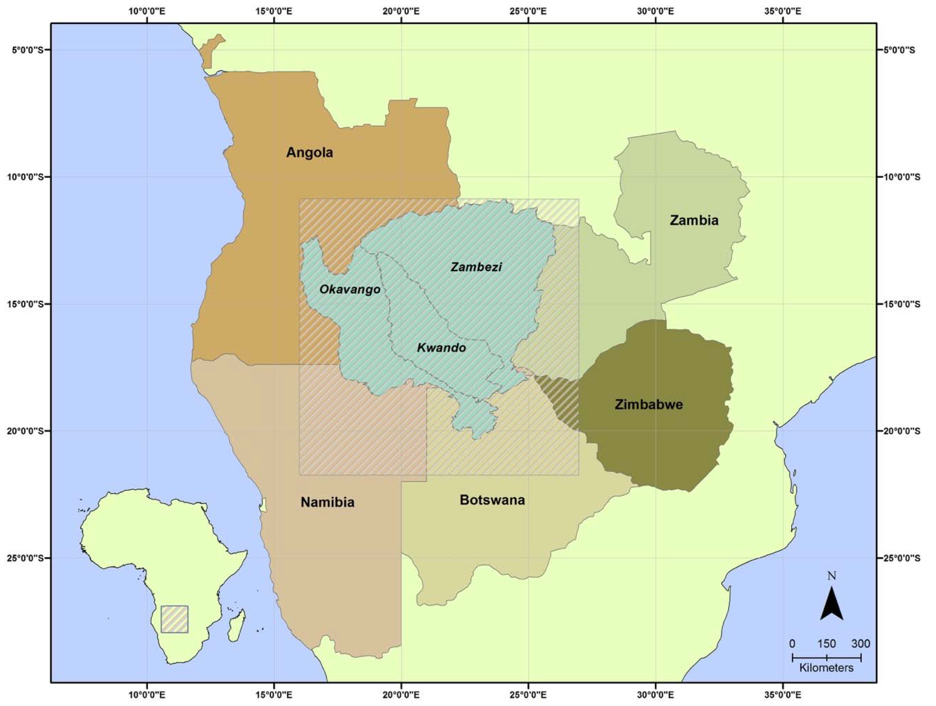
2.1. Study Area

The Okavango, Kwando, and upper Zambezi catchments (collectively called KAZA) combined cover 683,000 km2 of tropical and sub-tropical southern Africa (Figure 1) and MAP of 400–1500 mm. The southern portion is semi-arid, defined by low annual precipitation and high interannual variability, while totals and relative reliability increase northwards. Kalahari sands characterize the majority of the study region’s soils. Low topography in the south (especially Caprivi and northern Botswana) makes clear hydrologic separation of the catchments difficult. Historically, inter-basin water flowed eastward, as witnessed in May and June of 2008 (personal observation) but these systems have not connected consistently since the late 1970s. This correlates to a noted shift in global climate and an observed decrease in regional rainfall that has been identified as a possible reaction to atmosphere-ocean conditions in the Pacific Ocean [32,36,37,38].
Partly driven by, and partly in the context of significant climate variability and directional climate change, southern African countries are experimenting with varied resource management approaches, including the establishment of protected areas and community conservancies. Given the restricted viability of agriculture, conserving savanna ecosystems for ecological and economic reasons is crucially important to local peoples.
In this study, the data were aggregated to the basin level (Figure 1; Zambezi, Kwando and Okavango) such that both mean and variance of the time series were created. Drainage basins were used for this delineation rather than country for very specific reason. North to south across the three basins there are significant changes in climate regimes (temperature and precipitation), so these basins present this range in variation well. There are also differences in drivers of climate from east to west, which is well represented by the three basins. Overall, the climate drivers of spatial heterogeneity were broader scale and more significant that more localized drivers (e.g., population and country boundary).

2.2. Climate Data

Monthly global gridded high-resolution temperature and precipitation data were obtained from the University of Delaware. This time series stretches from 1901–2010 and was developed based on a large number of climate station data and data from the Global Historical Climate Network (GHCN2). These datasets were created via spatial interpolation at 0.5° resolution [39]. To indicate interpolation errors a station-by-station cross validation technique were employed [39]. In this study, the 1982–2010 portion of the time series was used for the calculation of long-term seasonal precipitation and air temperature metrics.

2.3. Remote Sensing

Only recently have remote sensing technologies developed sufficiently to meet the needs of ‘state-and-transition’ or ‘multiple stable state’ models [35] to systematically quantify and compare vegetation change [21]. The temporal frequency of remotely sensed data required to adequately describe major events is an important consideration in vegetation change detection, particularly in the tightly coupled vegetation–climate interactions of savanna ecosystems. Monthly time series of AVHRR- and MODIS-derived vegetation indices, now available from the early 1980s, hold considerable promise for the large-scale quantification of complex vegetation–climate dynamics and regional analyses of landscape change as related to global environmental changes [21]. A Normalized Difference Vegetation Index (NDVI) time series, which discriminates vegetation characteristics, including abundance, well in savanna regions [40,41,42,43,44] was utilized in a novel time series metric, which allows for both temporal and spatial specificity. NDVI is calculated as:
  NDVI = NIR Red NIR + Red
where NIR is reflectance in the near infrared portion and the RED is reflectance in the red portion of the electromagnetic spectrum.
The Global Inventory Monitoring and Modeling System Third Generation (GIMMS3g) NDVI data, generated from National Oceanic and Atmospheric Association’s (NOAA’s) AVHRR in the framework of the Global Inventory Monitoring and Modeling System (GIMMS) project at the NASA Goddard Space Flight Center, was utilized for the monthly time series. The data set spans from 1982 to 2010, and has a spatial resolution of 8 km and a temporal resolution of 15 days. Despite the corrections and temporal compositing, the GIMMS3g data still contains residual invalid measurements, well indicated by quality flags. Any pixel having less than 80% high-quality data throughout the entire time series, was excluded from the analysis. A gap-filling NDVI interpolation procedure was used for the time points with ‘poor’ quality flags. The GIMMS3g monthly NDVI data is compiled from the bi-monthly time-series using maximum value composite, these data were then aggregated to seasons: DJF = December, January, February; MAM = March, April, May; JJA = June, July, August; and SON = September, October, November. This study looks to understand the spatiotemporal vegetation trends across a large multi-country landscape, therefore requiring data that highlights landscape characteristics in the longest timeframe possible. AVHRR data provides such a data source, it was one of the first Earth imaging satellites parameterized for time series applications with sufficient repeat time and spatial coverage.

2.3.1. NDVI Metrics: Persistence, Seasonal NDVI, and Seasonal Cumulative NDVI

Using the NDVI time series a metric of vegetation persistence over time was developed [45,46,47]. Persistence, the increase or decrease in NDVI relative to a baseline status, was calculated on the time series to explore long-term spatial trends in vegetation. This research is incorporating the use of the persistence metric over other time-series type approaches such as regression analysis, wavelets, or fourier type techniques which have all been developed and used in recent years [48,49,50,51,52]. The concept for vegetation persistence comes from initial work by [53,54] both of whom argued for a benchmark approach to detecting time-series behaviors. Given the important role of climate and question of patterns of vegetation change in many regions—these ideas were integrated into the development of the directional persistence metric (D). This tool has the advantage of reporting at a pixel level scale, and facilitates the identification of areas of statistically significant changes across the landscape. The concept of using the benchmark or baseline conditions also allows the user to evaluate the role of a particular event or policy and its impacts on the landscape. A user can determine the level of statistical significance, split up the data based on their specific questions (e.g., monthly, annual etc.) and is computationally simple to run and easy to interpret. There is no assumption of linearity in the trend and the potential uses for such a technique are therefore quite diverse. As such, the use of the directional persistence metric allows for the detection of inter-annual changes that are different from what might be expected at random in seasonal NDVI, in a spatially explicit manner, and with predetermined critical levels of statistical significance. Persistence works by assigning a value of +1 or −1 to each year/season depending on whether the NDVI value exceeds the base value (here 1982–1986 seasonal values) or not. The summation of this dichotomous variable over the years is then mapped and analyzed statistically via linear regression and change point statistics.
Persistence was developed using monthly NDVI data compiled from AVHRR time series. Specifically, we utilize a measure called directional persistence, which indicates the overall direction of landscape change (increasing/decreasing) relative to a fixed benchmark condition (which could be tied to a climatic event, policy change, etc.) on a per pixel basis [45,46,47]. This metric is based on the principal of the random walk process, such that at any point in time, the likelihood of an increase versus a decrease in a value is identical (i.e., 0.5 probability) as this is a Bernouli random process. Each step is thus independent of the previous step, as in each value is compared to the baseline period only, and not to the previous time step. Therefore, the metric is the sum of the number of positive versus negative steps, which is very different from a regression type approach, which assumes a continuous linear process. As we know, in landscape change patterns are often discontinuous in time and space, and we wish to pick up these patterns more clearly, without the assumption of continuous processes.
For this study, seasonal baseline values are computed from 1982–1986, for comparison with the 24-subsequent seasonal NDVI values. This baseline period is representative of normal climate regimes across the region, i.e., no extreme multiyear drought events. Included in the baseline period is one El Niño event (1983), but throughout the rest of the time series there are other El Niño events, so having this in the baseline is representative of traditional climate regimes. The selection of the baseline period is obviously key to the interpretation of the results. Here, we wished to evaluate the longest period of time possible and to compare our results to what could be considered to be a typical baseline period. As such we selected a 5-year initial period to create our baseline. This was determined to be variable and representative in terms of climate, the main driver here, in that it did include an El Niño year. As you can see form the climate figures (Figure 2 and Figure 3), the period is not unusual in anyway and thus was deemed representative of a normal climate. As such, we then compared the following 24 years (1987 through to the end of 2010) to this initial period to allow us to investigate any potential trends or changes in landscape level vegetation persistence over this region. Of particular interest are clusters of similar patterns and variation over space in terms of significant results. We wanted to insure the longest possible record of data while also insuring the initial baseline period was representative of typical conditions. Figure 2 and Figure 3 highlight the seasonal climate trends throughout the entirety of the time series.
Directional persistence, D, is the cumulative direction of change over the time series relative to the fixed benchmark observation of NDVI (1982–1986 seasonal average), during a sequence of observations of a particular time period, in this case season (j), is derived as:
D j = i = 1 n 1 t i , j
  V c r i t < V i , j   : t i , j = + 1
  V c r i t > V i , j   : t i , j = 1
where Dj is the directional persistence for a given season j, and Vi,j is the seasonal NDVI (DJF, MAM, JJA, and SON), in year i, season j. For example, Vcrit is the critical benchmark NDVI value for observations made in MMA (j = 1), JJA (j = 2), SON (j = 3), or DJF (j = 4). A value of +1 is assigned to ti,j when the pixel for that year and season records a value of NDVI greater than the benchmark (Vcrit), and −1 for observations less than Vcrit. Theoretically, as NDVI is a continuous variable bounded by −1 and +1, identical values of NDVI are impossible. Predetermined critical levels of statistical significance, based on a random walk statistic, highlight the nature and extent of changes across the landscape beyond which might be expected at random and which are possibly indicative of degradation or other changes (see [45,46,47] for more details). The directional persistence (Dj) in this case yields a maximum range of −23 to +23 with the critical value of (α = 0.025) ±11 [45].
The persistence metric permits an objective identification of trends in vegetation across the globe for the last 29 years, highlighting regions of statistically significant change [21]. We will explore the spatial relationship between trends in persistence of vegetation and climate drivers at the regional scale to improve modeling of vegetation systems and thereby inform land use planning, management and policy, on regional and local scales.
Additionally, to analyze the interannual and intra-annual NDVI patterns two metrics were constructed that highlight the amplitude of greenness change. First, to analyze interannual variability, for each season (DJF, MAM, JJA, and SON) the NDVI values for the three-month seasonal (DJF, MAM, JJA, SON) period were summed. This seasonal NDVI has a theoretical range of +3 to −3. This seasonal NDVI time series was used to highlight the difference between seasonal greening patterns and the change in each season from year to year. Change point analysis was conducted to highlight the regimes across seasons over the time series (‘changepoint’ R package; [55]). Overall, the change point analysis looks to identify the location of multiple points of changes within a time series. At its simplest change point analysis/detection is an estimation of the point at which the statistical properties of a sequence of observations change [55]. According to the authors of [56], change point analysis essentially answers two questions key to time series analysis: (i) is there a statistically significant change in the distribution of values across the time series and (ii) when does this change occur? In this study, the change point analysis was developed based on a mean-variance statistical premise, meaning if the seasonal NDVI values of a pixel did not change significantly during our period of study the change point analysis would not highlight any inflection points. In contrast, if the pixel has seen statistically significant changes in vegetation production and therefore altered seasonal NDVI the result would be a new lower or high regime after that change. With such analyses there are three common methods for multiple change-point detection segmented neighborhood, binary segmentation, and the pruned exact linear time algorithm (PELT) [57]. In this study, the PELT algorithm was used as it has been more robust and computationally efficient. The change point analysis in the study was not constrained by a pre-defined number of regimes, instead statistically significant (p < 0.05) changes were defined by the analysis parameters. Meaning that across the basins and over the different seasons different numbers of change points were detected. Second, a total seasonal accumulation metric was calculated where every individual seasonal NDVI value was summed over time, such that a total cumulative NDVI (by season) was created. For such data, linear regression analysis techniques were utilized. By analyzing the linear trends in NDVI, we can illustrate changes over time, for example, the difference in total cumulative seasonal NDVI slope by basin.

3. Results

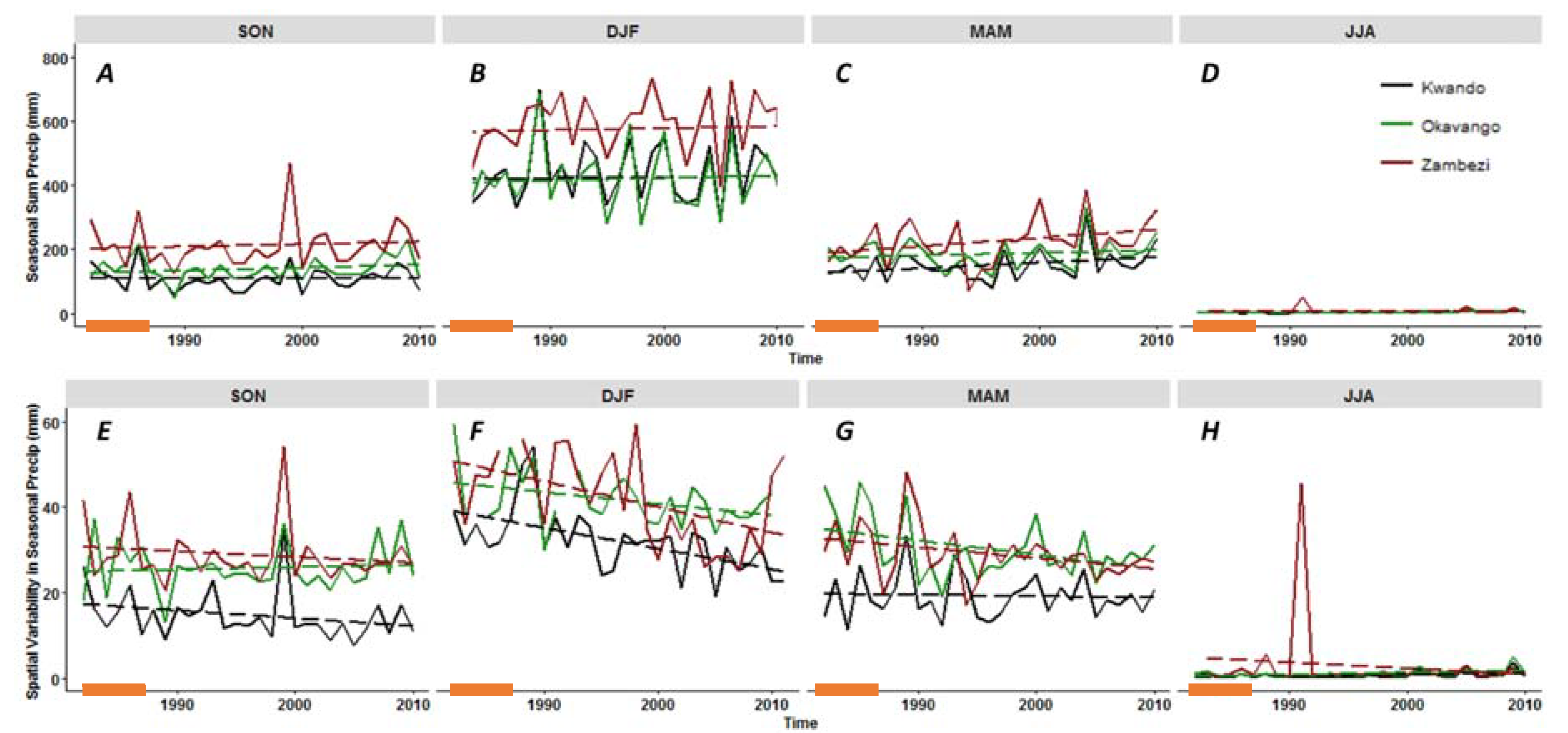
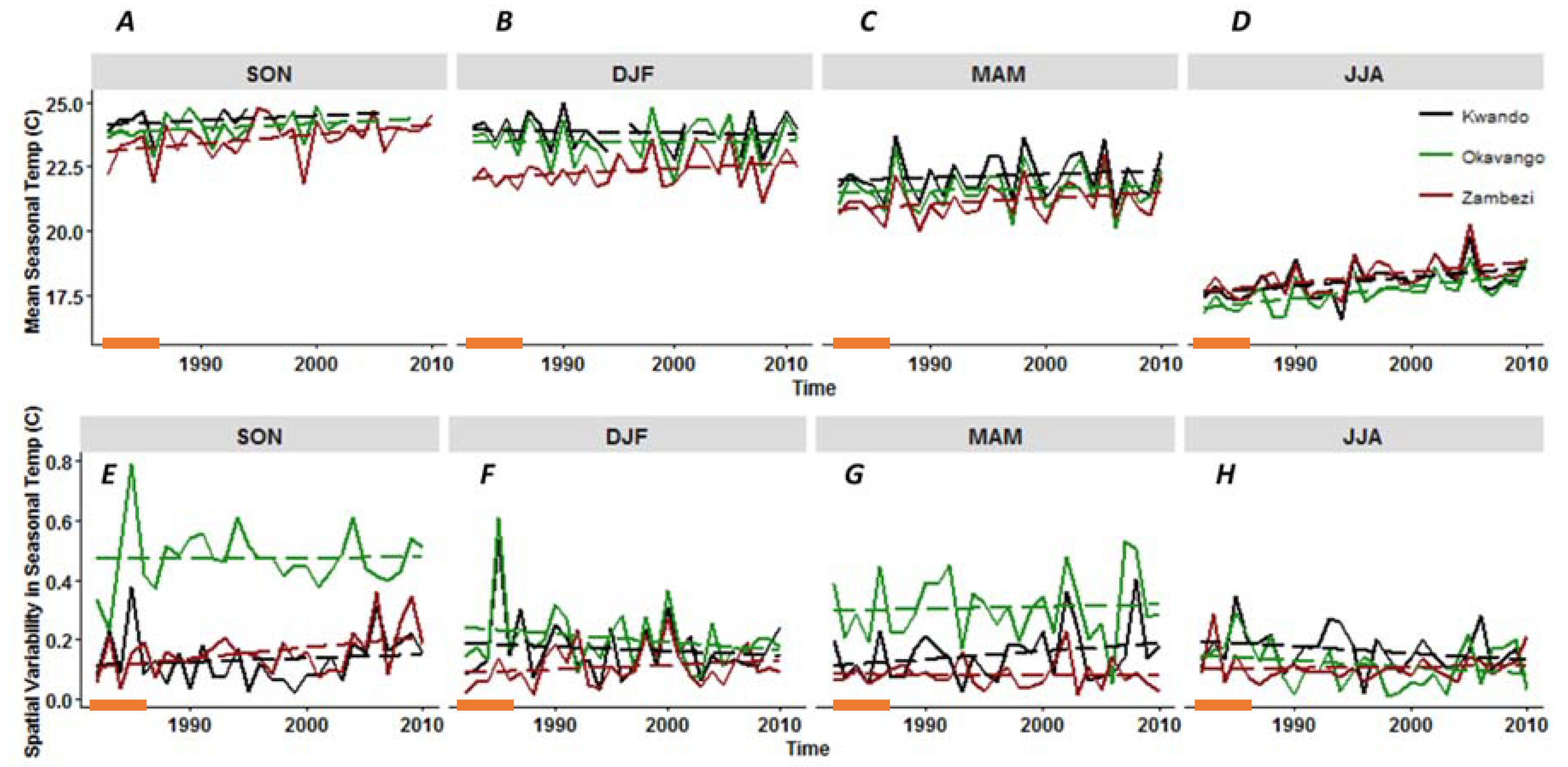
3.1. Climate Patterns

While precipitation is most commonly noted in the literature as the driving force of spatial heterogeneity across the landscape recent studies have emphasized the impact of temperature, in terms of constraining greening processes [19,20]. While both variables are highly influential in their own right, it is the cumulative impact of changing climate regimes that is driving landscape processes across savanna landscapes.
In terms of the precipitation regimes across the study area, we see very different seasonal trends. In JJA there is no change in the long-term total precipitation across any basin (Figure 2D). In the start of the wet season and throughout its progression (SON and DJF; Figure 2A,B), the total precipitation over time is relatively constant (not significantly increasing or decreasing), with trends holding across the three basins. Within these same seasons there are decreases in the spatial variability of precipitation, especially in DJF (Figure 2E,F). Towards the end of the wet season, in MAM, there is a notable increase in precipitation across all of the basins (Figure 2C). In this same season, the spatial variability of precipitation continues to decrease, especially in the Okavango and Zambezi basins. The decrease in variance of precipitation across the seasons reflects the decreasing spatial variability of precipitation patterns over the last 30 years (Figure 2E–H).
Temperature trends, unlike precipitation, have undergone changes across every season. In general, temperatures have steadily increased over time, in every basin of the study area (Figure 3A–D). The greatest change in temperature occurred in the dry season (JJA and SON), though wet season (DJF and MMA) temperature increases are also seen, except for the Kwando in DJF. Increasing temperatures will induce changes in the soil available moisture regime even at times of steady to slightly increasing precipitation. The change in the evaporative effect results in changes to the soil water balance system wide. Overall, the Zambezi basin had the steepest positive slope in terms of increasing temperature. Temperature variance across space, shows more varied changes and trends across seasons and basins (Figure 3E–H). In SON, there is no change in the variability, except for the Zambezi basin where an increasing trend is seen. Across all basins the spatial variability of temperatures decreased in DJF and JJA. Lastly, in MAM there is a slight increase in variability in the Kwando.

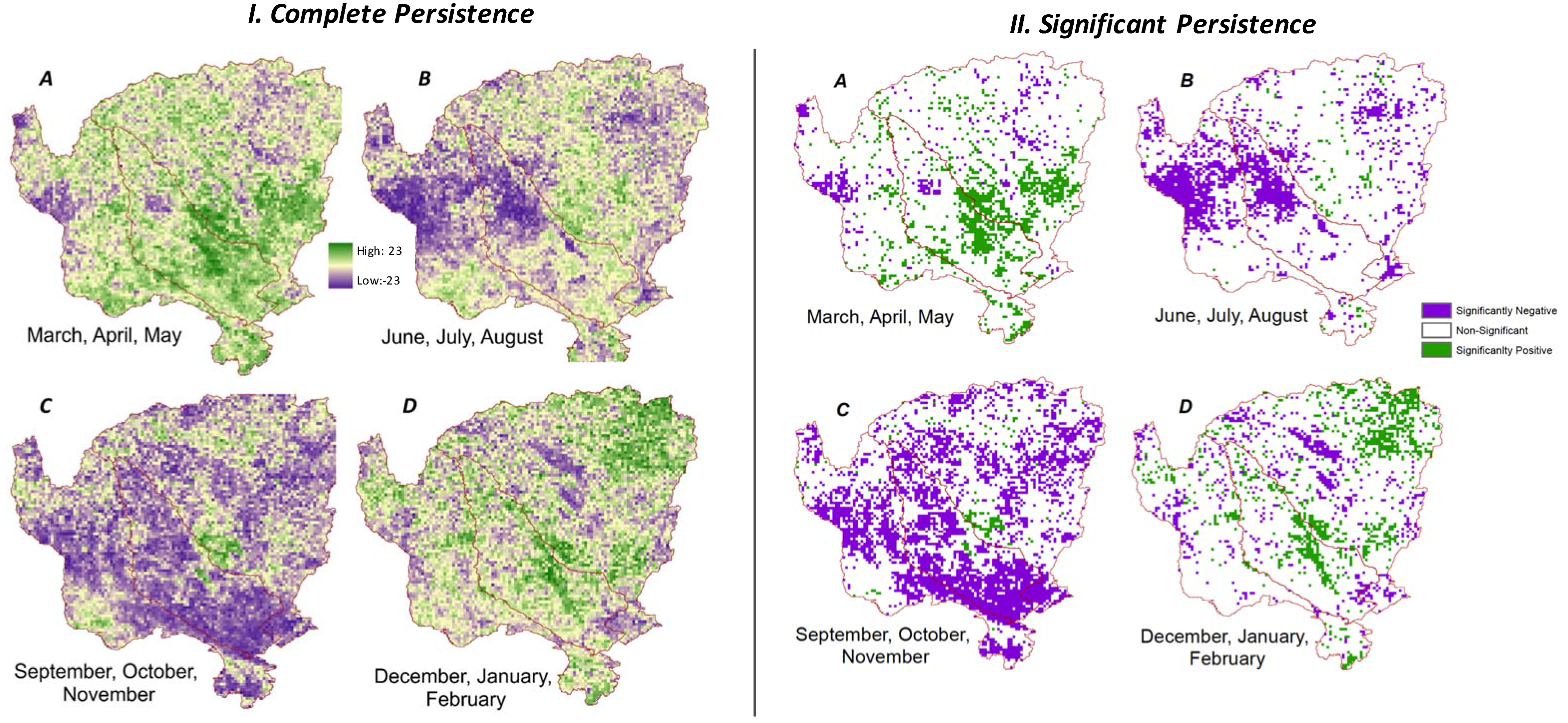
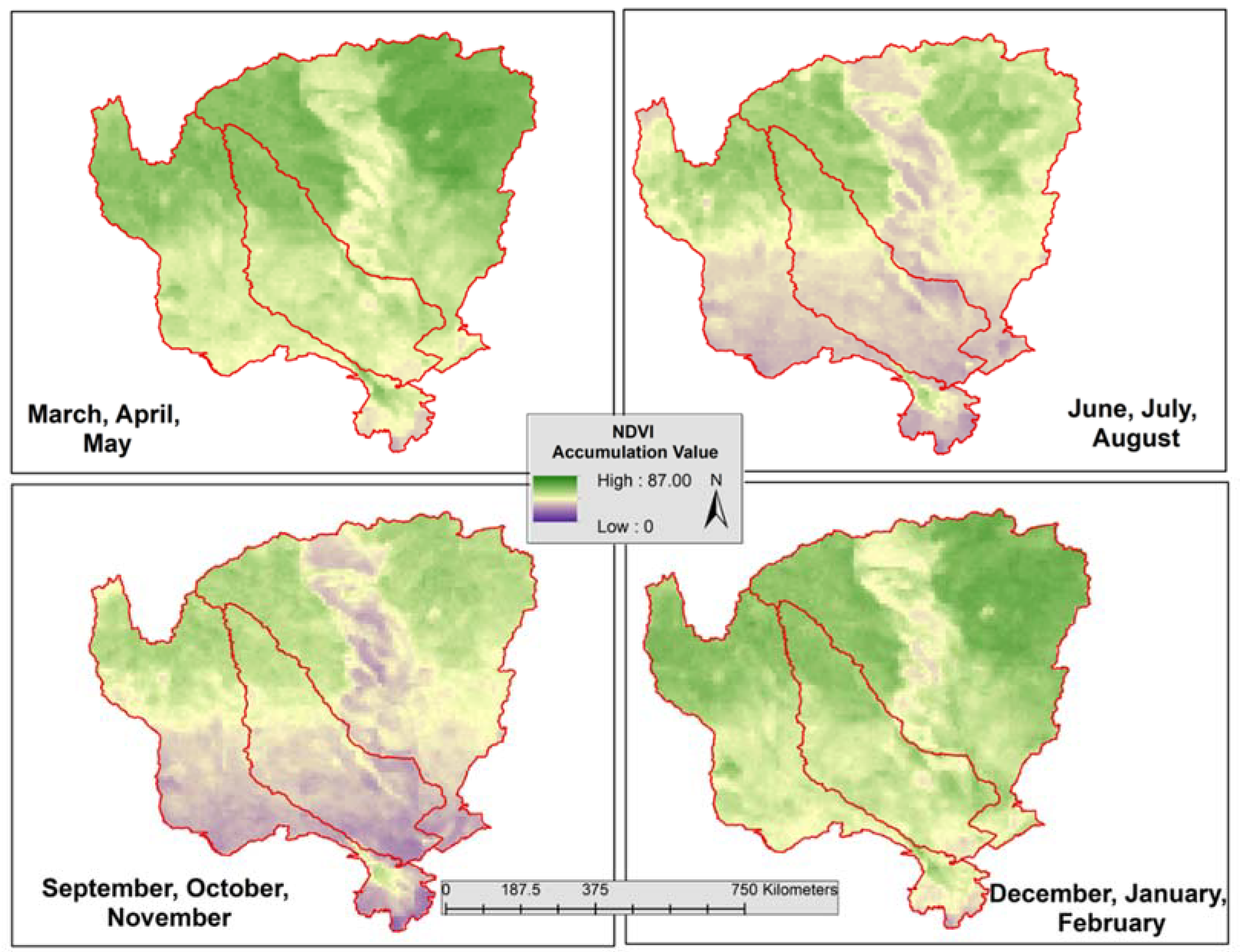
3.2. Directional Persistence

3.2.1. March, April, May Trends

Across the entire study area, there was a north-south pattern of persistence for MAM. The northern portions of the study area exhibited a more negative trend, whereas, the southern portion was associated with more positive persistence values (Figure 4). If we look at the trends per basin for statistically significant persistence values, the Okavango exhibits clusters of negative persistence values in the northern portion into Angola. The Delta portion of the Okavango mostly was comprised of positive persistence values. Overall, 15% of the Okavango exhibited positive persistence values and 11.1% negative persistence (Table 1). The Kwando basin, which was overwhelmingly positive in persistence (28.2%), showed a slight north to south difference in persistence values. Overall, across the Kwando only 3.6% of the landscape was statistically significant negative persistence, but the majority of this occurred in the northern portion of the basin as it reaches into Angola. The north to south variation continues in the Zambezi basin, with 18.4% of the landscape exhibiting positive persistence values and 7.1% having negative persistence (Table 1).

3.2.2. June, July, August Trends

During the dry season, from June through August, vegetation is senescing. Even taking that into account, the persistence values across the entire study area are mostly negative (Figure 4B). With the Okavango having 36.1% of its pixels as statistically significant negative values, the majority of which occur in Angola (Table 1). However, within/around the Okavango Delta itself, there is a mix of positive and negative persistence values. In the Kwando basin, 30.4% of the landscape is statistically significant negative persistence values. While the negative persistence values are spatially aggregated, there is a clear pattern of higher negative values within Angola. Approximately 0.4% of the Kwando is showing a statistically significant positive value in this dry season, which could be indicative of slower senescing of grasses. Lastly, in the Zambezi there is a distinct trend in the persistence values. Statistically significant negative values occur across 17% of this catchment, whereas the positive values only occur across 4.2% of the catchment (Table 1). There could be multiple drivers for this spatial aggregation of persistence but it appears that low-lying (potentially seasonally-flooded) regions can explain the differential greening.

3.2.3. September, October, November Trends

Like the JJA season, a negative persistence trend is seen across the majority of the study area in SON (Figure 4C). This season is representative of the latter portion of the dry season and the onset of the wet season. Given the delay in precipitation starting [58] and so later greening of vegetation, little greening would be expected in this season. The change in NDVI that is occurring is indicative of the grass component. In terms of persistence values across the three catchments, 38–68% of the landscape has statistically significant and negative persistence values (Table 1). The majority of both the Okavango and Kwando basins exhibit negative values of varying degrees of statistical significance. The Zambezi portion of the study area near the border between Angola and Zambia demonstrates positive persistence of vegetation, though elsewhere the trend is predominately negative.

3.2.4. December, January, February Trends

Across the entire study area in the DJF season there is no distinct persistence trend, as seen in other seasons (Figure 4D). In each of the basins there are clusters of positive and negative persistence values. For example, positive persistence clusters are seen in the Okavango Delta and at the Angola/Zambia border stretching into northern Namibia. Overall between 9–20% of the landscape has statistically significant positive persistence values, whereas, 7–15% has statistically significant negative values (Table 1).

3.2.5. Overarching Trends

The majority of the study area exhibited statistically significant persistence trends across the seasons (Figure 4; Table 1). The previously mentioned breakdowns by percentage did not include areas where the persistence was not statistically significant. In several portions of the study area we see a switch from season to season in terms of the persistence values. The statistically significant positive or negative persistence are not indicative of complete landscape change rather they highlight seasonal variation in NDVI patterns. To further understand the drivers and temporal trend the NDVI accumulation metric is utilized.

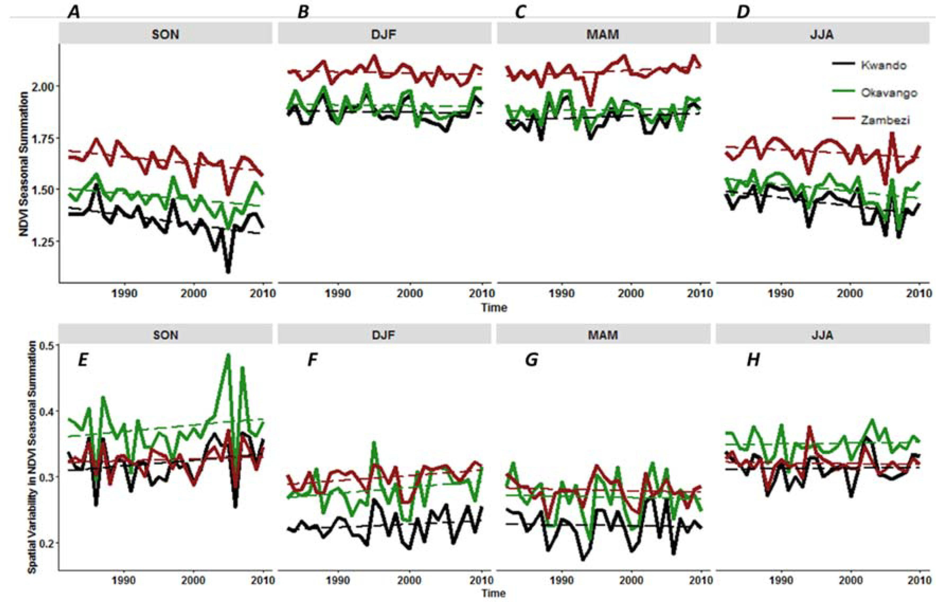
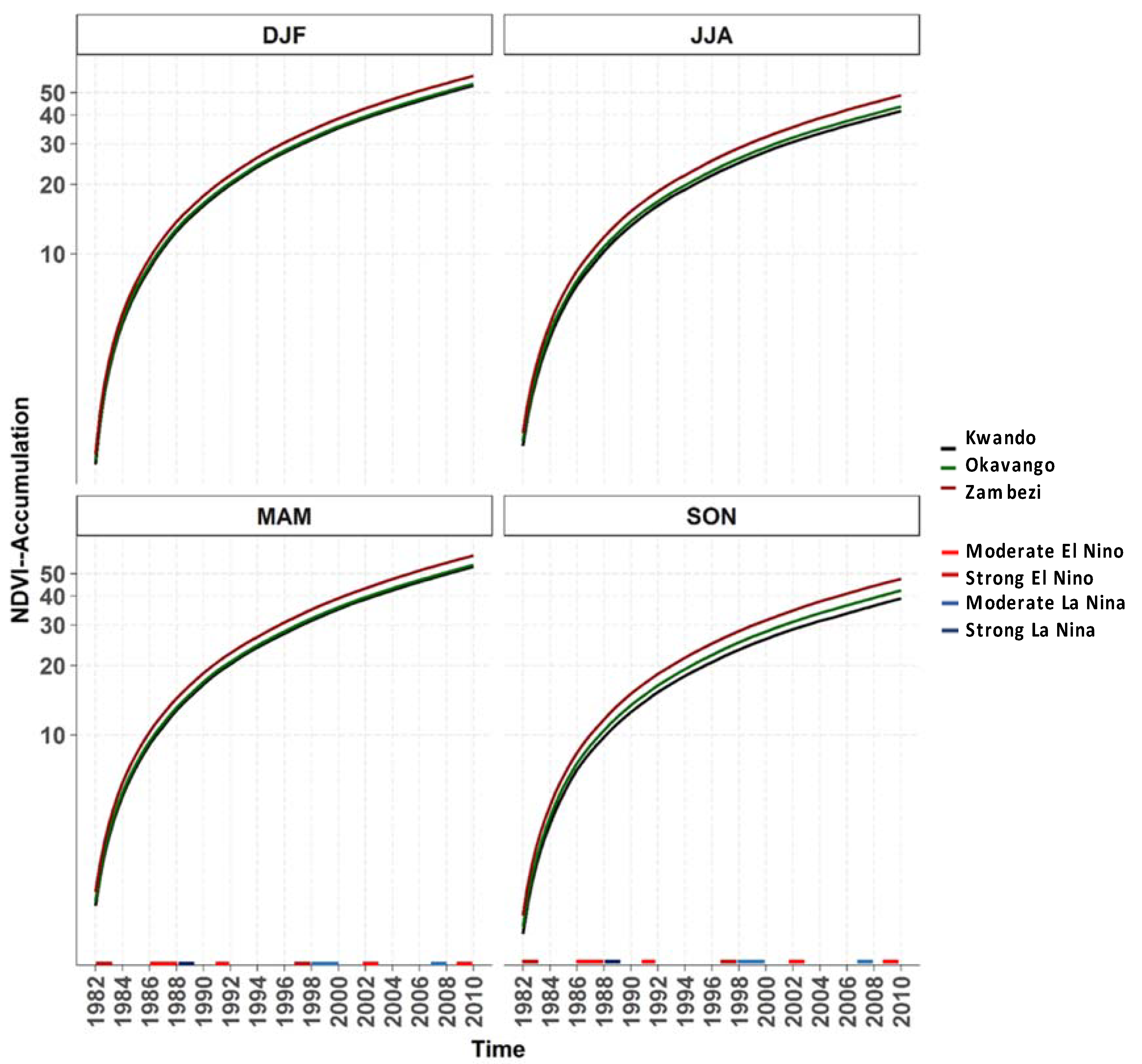
3.3. Seasonal Accumulation Patterns

The seasonal NDVI accumulation metric (Figure 5) illustrates the seasonality of the system with the dry season (Figure 5B,C) and the wet season (Figure 5A,D) showing very different trends. Additionally, the metric highlights the differing precipitation trends across the study area, driven by the migration of the Inter Tropical Convergence Zone (ITCZ) and its effect on landscape greening (Figure 5). In SON, the end of the dry season and start of the wet, we see that the northern portion of the study area exhibits high accumulation values (Figure 5C). This portion of the study area is the first impacted by the southwards migration of the ITCZ. Across DJF we see that more of the study area is exhibiting high accumulation values. By this time in the season the lag between the onset of precipitation and vegetation greening has passed. In DJF, we would expect a ramp up of vegetation productivity and that is what is seen. MAM exhibits similar accumulation values as DJF, though in the southern portion of the study area there are noted declines across the two seasons. This decline can be associated, again, with the change in the ITCZ location. Lastly, in JJA, lower accumulation values are seen across the landscape, but especially for the southern portion. This is a time of water stress in the region and low productivity. If we look at this NDVI accumulation temporally, in addition to spatially (Figure 5), we can see what is driving the positive and negative persistence values.

3.3.1. Time Series Analysis

When coupling the persistence and previously described climate trends, we can explain in detail the NDVI time series trends. In the wet season, spanning DJF and MAM, across all catchments, a flat to slightly increasing NDVI trend is seen over time (Figure 6). This increasing trend of greenness is linked with the trend in precipitation. Additionally, if we link back with persistence, we see that these two seasons both have high proportions of the landscape with statistically significant positive persistence values. Several years stand out across all basins as having anomalously high NDVI, mostly in the MAM season, including: 1988, 1998, 1999, and 2010. The latter three years were moderate La Niña years. In 1987, 1992, and 2002, all of which are El Niño years, there were low seasonal NDVI values.
In the dry season, the combination of increasing temperatures and little to no precipitation results in diminished soil available moisture and therefore less potential for vegetation to green. In the dry seasons (JJA and SON) we see that NDVI values have a decreasing linear trend over time (Figure 6). These seasons were also when negative persistence values were seen across the majority of the landscape. This suggests that the dry season is getting drier and the vegetation cover is either senescing faster, dying off, or converting to a less biologically productive and potentially lower photosynthetically active cover type.
Overall, the pattern of the directional persistence highlights the all-encompassing impact of both abiotic and biotic drivers of landscape change. However, teasing apart the pattern of persistence requires an evaluation of the main drivers of spatial heterogeneity, in this case climate, and the trends in the NDVI themselves. Of the three catchments, the Zambezi receives the highest mean annual precipitation, which has been maintained or increased across the time series, but has also seen large increases in temperature across every season. The combination of sustained precipitation and increased temperatures leads to long term decreases in water availability. Hand in hand the increased variability in soil available moisture has led to large-scale changes in greening as seen in the directional persistence and seasonal NDVI. The seasonal NDVI has shown greater senescence or browning down of vegetation over time, especially in SON and JJA. Like with the Zambezi, in the Kwando and Okavango catchments the directional persistence and seasonal NDVI show broad scale decreases in vegetation in SON and JJA but a more mixed spatial and temporal pattern in DJF and MAM, all of which can be linked to the pattern and spatial variability in the climate variables.
If we look at the overall trajectory of the cumulative NDVI the aforementioned patterns are highlighted, as we see differential slopes across basins and seasons (Figure 7; Table 2). The slope of the cumulative NDVI gives a quantitative output indicative of the greening trajectory. Across all seasons the Zambezi catchment had the steepest linear slope (SON = 1.64, DJF = 2.06, MAM = 2.14, and JJA = 1.68), whereas the Kwando catchment has the smallest slope in every season, though the Okavango has similar slopes to the Kwando. The NDVI accumulation highlights not only the different degrees of greening across the basin but also the degree of seasonal variation in greening.

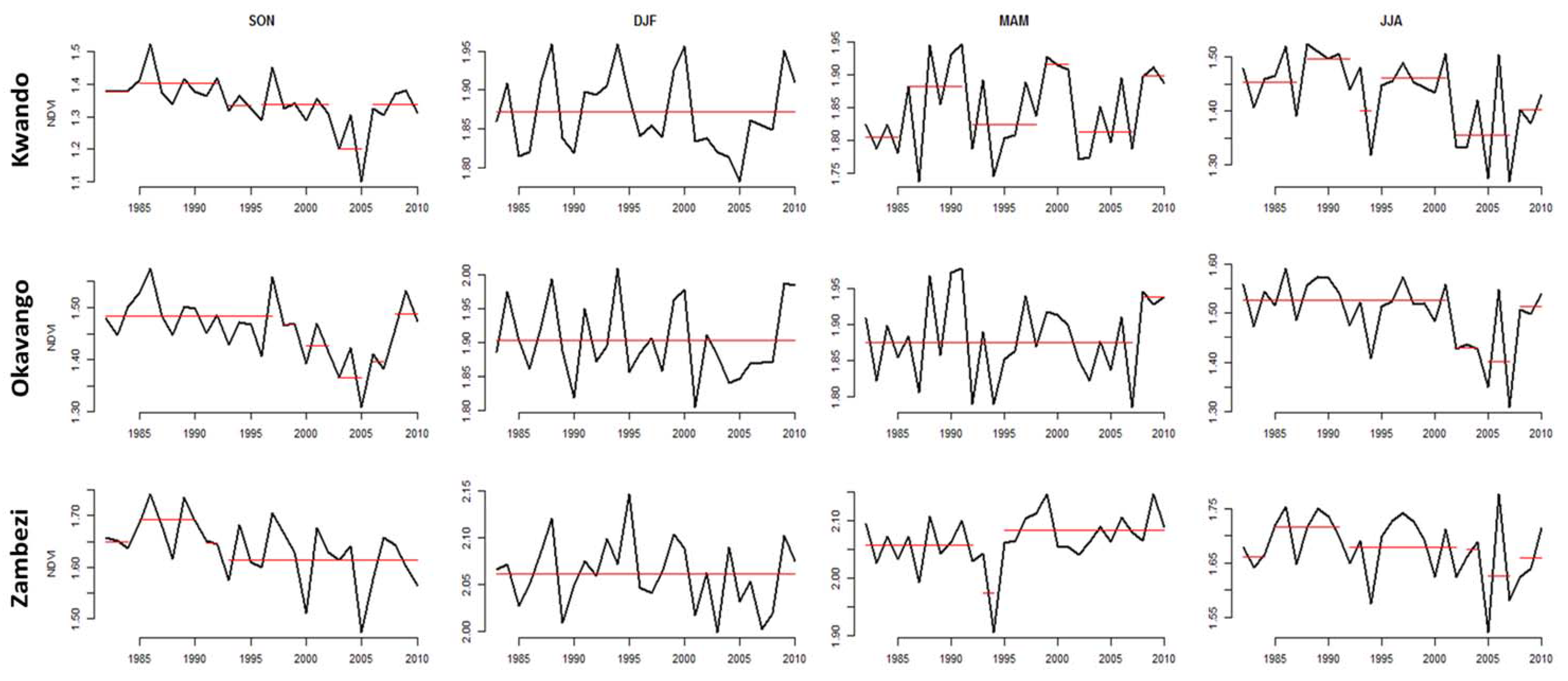
3.3.2. Change Point Analysis

Through the persistence and other NDVI metrics we have highlighted the degree to which vegetation greening has changed across the three basins and even pinpointed years of greatest change. To relate the climate trends with the persistence and NDVI accumulation, a change point analysis was undertaken. Such analyses highlights regimes across the basins in each season for the NDVI data.
The NDVI seasonal values show distinctly different regimes over time according to the change point analysis (Figure 8). In the SON season, we see that two distinct regimes occur across all basins with the earlier portion of the time series exhibiting higher NDVI values compared to the latter portion. The one season not exhibiting changes in the long-term greening regimes is DJF. In this season, all basins are showing high interannual variability but consistency in the long-term mean. In the latter portion of the wet season (MAM) there are no consistent regime changes across the basins. The dry season, the height of which is exhibited in JJA, shows a similar trend as SON, meaning that the latter portion of the time series has lower NDVI values than the beginning.

4. Discussion

4.1. Physiological Trends and Drivers of Spatial Heterogeneity

The ecological, environmental, and social dynamics of the KAZA study area have been extensively studied for decades and the story echoed in the majority of articles is that climate is the key driver of ecosystem function for the region [19,20,34,46,59]. In this article, via novel time series remotely sensed metrics, we emphasize that climate is the main driver of spatial heterogeneity of vegetation cover in the study area and further decompose the driving forces to look at the impacts of temperature and precipitation separately on the landscape. The climate analysis highlights changes to both precipitation (spatially and temporally variable pattern), temperature (increasing trend), and a change in the overall spatial variability of these drivers of spatial heterogeneity. With increased temperatures, there is a greater evaporative demand that is not offset by the precipitation inputs. During the time frame of this analysis in three seasons (SON, DJF, and MAM) there were increases, in total precipitation. Additionally, in these seasons there were large decreases in the spatial variability of precipitation, though this trend differed across the basins. However, in JJA there was no distinct change in the regime of seasonal precipitation, though the variability greatly decreased. The major change in climate for the area is related to temperature, as higher temperatures were seen in almost all basins across all seasons. While the precipitation was maintaining the long-term trend or slightly increasing, the increased temperature will result in a large reduction in available soil moisture and will therefore impact the greening trends exhibited.
In both the persistence and the NDVI accumulation, we can infer the impact of change in available soil moisture. The landscape-level negative persistence values and changing regimes in the NDVI accumulation for SON, MAM, and JJA highlight the increased aridity of the KAZA region, even with the increased precipitation.
Across southern Africa, moisture availability has a strong positive relationship with vegetation abundance [7,14,21]. Across seasons and years, we show that vegetation trends, via persistence and both NDVI metrics, have decreased in terms of amount and greenness, perhaps an indication of degradation. While we cannot specifically indicate which vegetation, structural type is experiencing the reduction in cover, we can hypothesize based on structural group response to long-term reduction in available soil moisture. The reduction in cover can be linked to either a total loss of vegetation (increased bare ground) or a transition in the dominant vegetation cover. As the authors of [1] state, the circumstances leading to state or demographic transitions differ across savannas, and interannual variability in rainfall often triggers such transitions. In times of high precipitation, grass productivity is increased, promoting fire and leading to the suppression of woody vegetation sapling growth. This implies that the accumulation of non-woody vegetation, especially C4 grasses, is linearly and tightly controlled by the intra-annual variability in the start of the wet season and the amount of precipitation [1]. However, in the more arid savannas, increased precipitation promotes tree establishment too, sometimes suppressing grass development [1]. Recent research on the drivers of landscape change across southern Africa highlights the importance of temperature in dictating potential vegetation abundance via limitations in soil moisture because of increased evaporation or increased fire susceptibility [19]. The increased temperatures seen across all months of all basins would alter the water balance regime of the region, leading to an overall decrease in soil moisture availability. The cumulative impact of increased temperature and alterations to precipitation amounts and variability will have differential impact on landscape patterns across savanna ecosystems.

4.2. Climate Change

In a region, such as KAZA, where humans rely on rain-fed agriculture and the resources extracted from the savannas, there are potentially significant economic problems in the future. Currently, there is no specific climate change policy in place, but in Namibia a climate advisory committee was established in 1997 [33]. While there have been several attempts at the international level, i.e., Kyoto Protocol and Copenhagen, none of these policies are directly seeking to combat the water scarcity problems facing southern Africa.
In terms of the resilience of savanna landscapes, climate change induced alterations in water availability and soil water balance may exacerbate the complex states, pushing the system to cross tipping points, which for this study area would result in more arid to hyper arid conditions [60]. There is a strong correlation between climate variables (precipitation and temperature) and vegetation abundance/greenness. With projected increases in precipitation variability, decreases in overall precipitation amount, and increases in precipitation-related extreme events, associated vegetation changes should also be expected [34]. It has been suggested that high variance at the arid end of the precipitation gradient, and not low mean annual rainfall is what matters most in terms of woody vegetation growth [60]. Under projected climate change conditions, where increased variability is predicted, the resultant climate would have major repercussions on tree cover. For example, the authors of [14] found that changes in precipitation may considerably affect distribution and dynamics of savanna, potentially leading to changes in state or further bush encroachment. Since savannas are anticipated to be among the ecosystems that are most sensitive to future climate changes [61,62,63], a thorough understanding of factors that structure savanna communities is necessary in order to guide management efforts [14,64,65].
How differing vegetation types (C3 and C4 plants) respond to climate change is a key theme in current ecological research. The authors of [66] found that elevated CO2 concentrations should favor tree and woody plants (C3 vegetation) over herbaceous species (C4) in Africa. The basics of plant physiology are the causation for such projected woody plant dominance under climate change conditions. Essentially, woody vegetation uses the C3 photosynthetic pathway, which is favored under higher CO2 concentrations [11]. Conversely, most herbaceous vegetation in grasslands and savannas utilize the C4 photosynthetic pathway [1]. Temperature also influences tree-versus-grass ratios in ecosystems, though there is a general consensus in the literature that projected CO2 changes overwhelms the impacts of changing temperatures [66]. In general, it is thought that with higher temperatures, C4 grasses will dominate over C3 trees [1]. With only a slight increase in tree cover, a cascading effect can take place to make woody vegetation suppress herbaceous vegetation. More woody vegetation will suppress herbaceous production through both light competition and decreased fire sensitivity [66]. As the authors of [66] stated, even minor increases in woody vegetation cover, “further increases the likelihood of the system tipping from a C4-dominated state to a C3-dominated state”, essentially changing to a woody savanna or woodland. Under climate change overarching global projections indicate an increase in woody vegetation, and the potential for grassland ecosystems to become more savanna/woodland systems.

4.3. Implications for the Developed NDVI Metrics

Persistence and the associated NDVI metrics were developed at a coarse spatial resolution using AVHRR data. This data, while coarse and not ideal for plant community level work, is suitable for detecting trends across the landscape given its high temporal frequency and longer temporal extent. In order to address specific plant community assemblages and their long-term trend and persistence fine level remotely sensed data and in-depth field studies are essential.

5. Conclusions

Numerous articles have focused on the impacts of soil moisture (precipitation and temperature) on vegetation patterns in savanna landscapes. In this study, we show that climate induced reductions in NDVI (i.e., degradation or biomass decline) have had large spatial and temporal impacts across the Kwando, Okavango, and Zambezi catchments of southern Africa, regions deemed arid to semi-arid savannas. We conclude that over time there have been alterations in the available soil moisture resulting from increases in temperature in every season. Such changes in the ecosystem dynamics of all three basins are leading to system-wide changes in landscape greening patterns. From March to August we show that vast portions of the study area have statistically significant negative persistence values, indicative of increased browning down of vegetation, whereas DJF and MAM illustrate a higher proportion of statistically significant positive persistence values. Given the changing climate regimes and resulting persistence values, our results could be indicating a shift in the landscape. As climate change further impacts this and similar landscapes across Southern Africa, significant changes in vegetation cover amount and type will likely occur. Managers need to plan for such shifts in vegetation type and also in timing and frequency of extreme events. Current trends over the last thirty plus years can be used to highlight the types of changes already occurring, in order to predicate future planning and management regimes. The need to better understand these changes and explain their behavior is critical, as climate changes continue to occur across this region, and future climate scenarios are predicted to increase even more in terms of absolute increase in temperature and increased variability of precipitation. This landscape is changing and we need to manage and plan for what the future will bring.

Author Contributions

J.S. and P.W. conceived and developed the persistence metrics and associated statistical tests. E.L.B. and J.S. developed the seasonal accumulation and cumulative NDVI metrics and determined the appropriate statistical tests. The article was jointly written by E.L.B. and J.S. All figures, graphs, and statistical tests were completed by E.L.B. All authors contributed to the writing and editing of this article.

Funding

This research was funded from a NASA LCLUC grant; proposal NNX09AI25G: Understanding and Predicting the Impact of Climate Variability and Climate Change on Land Use and Land Cover Change Via Socio-Economic Institutions in Southern Africa.

Acknowledgments

The authors would like to thank the reviewers and editors for their timely review of our article. Numerous people assisted in developing the persistence metric and this article and we would like to thank them including: Likai Zhu and Cerian Gibbes.

Conflicts of Interest

The authors declare no conflict of interest.

Abbreviations

The following abbreviations are used in this manuscript:
MODISModerate Resolution Imaging Spectroradiometer
AVHRRAdvanced Very High-Resolution Radiometer
GHCN2Global Historical Climate Network
MAPMean Annual Precipitation
NDVINormalized Difference Vegetation Index
PELTPruned Exact Linear Time
UNFCCCUnited Nations Framework Convention on Climate Change

References

  1. Bond, W.J. What Limits Trees in C4 Grasslands and Savannas? Annu. Rev. Ecol. Evol. Syst. 2008, 39, 641–659. [Google Scholar] [CrossRef]
  2. Scholes, R.J. Convex relationships in ecosystems containing mixtures of trees and grass. Environ. Resour. Econ. 2003, 26, 559–574. [Google Scholar] [CrossRef]
  3. Sankaran, M.; Ratnam, J.; Hanan, N. Tree–grass coexistence in savannas revisited—Insights from an examination of assumptions and mechanisms invoked in existing models. Ecol. Lett. 2004, 7, 480–490. [Google Scholar] [CrossRef]
  4. Scholes, R.J.; Archer, S.R. Tree-grass interactions in savannas. Annu. Rev. Ecol. Syst. 1997, 28, 517–544. [Google Scholar] [CrossRef]
  5. Walter, H.; Burnett, J.H.; Mueller-Dombois, D. Ecology of Tropical and Subtropical Vegetation; Oliver & Boyd: Edinburgh, UK, 1971. [Google Scholar]
  6. Lehmann, C.E.; Anderson, T.M.; Sankaran, M.; Higgins, S.I.; Archibald, S.; Hoffmann, W.A.; Hanan, N.P.; Williams, R.J.; Fensham, R.J.; Felfili, J.; et al. Savanna vegetation-fire-climate relationships differ among continents. Science 2014, 343, 548–552. [Google Scholar] [CrossRef] [PubMed]
  7. Sankaran, M.; Ratnam, J.; Hanan, N. Woody cover in African savannas: The role of resources, fire and herbivory. Glob. Ecol. Biogeogr. 2008, 17, 236–245. [Google Scholar] [CrossRef]
  8. Sugihara, G.; May, R.; Ye, H.; Hsieh, C.; Deyle, E.; Fogarty, M.; Munch, S. Detecting Causality in Complex Ecosystems. Science 2012, 338, 496–500. [Google Scholar] [CrossRef] [PubMed]
  9. Kgope, B.; Bond, W.; Midgley, G.F. Growth responses of African savanna trees implicate atmospheric [CO2] as a driver of past and current changes in savanna tree cover. Austral Ecol. 2010, 35, 451–463. [Google Scholar] [CrossRef]
  10. Ellis, J.E.; Swift, D.M. Stability of African pastoral ecosystems: Alternate paradigms and implications for development. Rangel. Ecol. Manag. J. Range Manag. Arch. 1988, 41, 450–459. [Google Scholar] [CrossRef]
  11. Buitenwerf, R.; Bond, W.J.; Stevens, N.; Trollope, W.S.W. Increased tree densities in South African savannas: >50 years of data suggests CO2 as a driver. Glob. Chang. Biol. 2012, 18, 675–684. [Google Scholar] [CrossRef]
  12. Makarieva, A.M.; Gorshkov, V.G. Biotic pump of atmospheric moisture as driver of the hydrological cycle on land. Hydrol. Earth Syst. Sci. Discuss. 2006, 3, 2621–2673. [Google Scholar] [CrossRef]
  13. Gillson, L.; Hoffman, M.T. Ecology. Rangeland ecology in a changing world. Science 2007, 315, 53–54. [Google Scholar] [CrossRef] [PubMed]
  14. Sankaran, M.; Hanan, N.P.; Scholes, R.J.; Ratnam, J.; Augustine, D.J.; Cade, B.S.; Gignoux, J.; Higgins, S.I.; Le Roux, X.; Ludwig, F.; et al. Determinants of woody cover in African savannas. Nature 2005, 438, 846–849. [Google Scholar] [CrossRef] [PubMed]
  15. Good, S.P.; Caylor, K.K. Climatological determinants of woody cover in Africa. Proc. Natl. Acad. Sci. USA 2011, 108, 4902–4907. [Google Scholar] [CrossRef] [PubMed] [Green Version]
  16. Seghieri, J.; Vescovo, A.; Padel, K.; Soubie, R.; Arjounin, M.; Boulain, N.; de Rosnay, P.; Galle, S.; Gosset, M.; Mouctar, A.H.; et al. Relationships between climate, soil moisture and phenology of the woody cover in two sites located along the West African latitudinal gradient. J. Hydrol. 2009, 375, 78–89. [Google Scholar] [CrossRef]
  17. Vanacker, V.; Linderman, M.; Lupo, F.; Flasse, S.; Lambin, E.F. Impact of shortterm rainfall fluctuation on interannual land cover change in sub-Saharan Africa. Glob. Ecol. Biogeogr. 2005, 14, 123–135. [Google Scholar] [CrossRef]
  18. Mayer, A.L.; Khalyani, A.H. Grass Trumps Trees with Fire. Science 2011, 334, 188–189. [Google Scholar] [CrossRef] [PubMed]
  19. Campo-Bescós, M.A.; Muñoz-Carpena, R.; Kaplan, D.A.; Southworth, J.; Zhu, L.; Waylen, P.R. Beyond precipitation: Physiographic gradients dictate the relative importance of environmental drivers on savanna vegetation. PLoS ONE 2013, 8, e72348. [Google Scholar] [CrossRef] [PubMed]
  20. Campo-Bescós, M.A.; Muñoz-Carpena, R.; Southworth, J.; Zhu, L.; Waylen, P.R.; Bunting, E. Combined spatial and temporal effects of environmental controls on long-term monthly NDVI in the southern Africa Savanna. Remote Sens. 2013, 5, 6513–6538. [Google Scholar] [CrossRef]
  21. Southworth, J.; Zhu, L.; Bunting, E.; Ryan, S.J.; Herrero, H.; Waylen, P.R.; Hill, M.J. Changes in vegetation persistence across global savanna landscapes, 1982–2010. J. Land Use Sci. 2016, 11, 7–32. [Google Scholar] [CrossRef]
  22. Bucini, G.; Hanan, N. A continental-scale analysis of tree cover in African savannas. Glob. Ecol. Biogeogr. 2007, 16, 593–605. [Google Scholar] [CrossRef]
  23. Murphy, B.P.; Bowman, D.M. What controls the distribution of tropical forest and savanna? Ecol. Lett. 2012, 15, 748–758. [Google Scholar] [CrossRef] [PubMed] [Green Version]
  24. Seaquist, J.W.; Hickler, T.; Eklundh, L.; Ardö, J.; Heumann, B.W. Disentangling the effects of climate and people on Sahel vegetation dynamics. Biogeosciences 2009, 6, 469–477. [Google Scholar] [CrossRef] [Green Version]
  25. Houghton, J.T.; Ding, Y.; Griggs, D.J.; Noguer, M.; van der Linden, P.J.; Dai, X.; Maskell, K.; Johnson, C.A. The IPCC Report 2001; IPCC: Geneva, Switzerland, 2000; Volume 463, p. 255. [Google Scholar]
  26. Niang, I.; Abdrabo, M.A.; Essel, A.; Lennard, C.; Padgham, J.; Urquhart, P. Africa. In Climate Change 2014: Impacts, Adaptation, and Vulnerability. Part B: Regional Aspects. Contribution of Working Group II to the Fifth Assessment Report of the Intergovernmental Panel on Climate Change; Barros, V.R., Field, C.B., Dokken, D.J., Mastrandrea, M.D., Mach, K.J., Bilir, T.E., Chatterjee, M., Ebi, K.L., Estrada, Y., Genova, R.C., et al., Eds.; Cambridge University Press: Cambridge, UK; New York, NY, USA, 2014; pp. 1199–1265. [Google Scholar]
  27. McCarthy, J.J.; Canziani, O.F.; Leary, N.A.; Dokken, D.J.; White, K.S. Climate Change 2001: Impacts, Adaptation, and Vulnerability; Cambridge University Press: Cambridge, UK, 2001. [Google Scholar]
  28. Parry, M.L. Climate Change 2007: Impacts, Adaptation and Vulnerability: Working Group II Contribution to the Fourth Assessment Report of the IPCC Intergovernmental Panel on Climate Change; Cambridge University Press: Cambridge, UK, 2007; ISBN 978-0-521-88010-7. [Google Scholar]
  29. Hernes, H.; Dalfelt, A.; Berntsen, T.; Holtsmark, B.; Næss, L.O.; Selrod, R.; Aaheim, H.A. Climate Strategy for Africa; CICERO Report; CICERO: Oslo, Norway, 1995. [Google Scholar]
  30. Ringius, L.; Downing, T.; Hulme, M.; Waughray, D.; Selrod, R. Climate Change in Africa: Issues and Challenges in Agriculture and Water for Sustainable Development; CICERO Report; CICERO: Oslo, Norway, 1996. [Google Scholar]
  31. Susan, S. (Ed.) Climate Change 2007—The Physical Science Basis: Working Group I Contribution to the Fourth Assessment Report of the IPCC; Cambridge University Press: Cambridge, UK, 2007; Volume 4. [Google Scholar]
  32. Gaughan, A.E.; Waylen, P.R. Spatial and temporal precipitation variability in the Okavango–Kwando–Zambezi catchment, southern Africa. J. Arid Environ. 2012, 82, 19–30. [Google Scholar] [CrossRef]
  33. McGann, J. The current status of unfccc article 6 work program implementation in Namibia. In Proceedings of the African Workshop on Article, Banjul, The Gambia, 28–30 January 2004. [Google Scholar]
  34. Cui, X.; Gibbes, C.; Southworth, J.; Waylen, P. Using Remote Sensing to Quantify Vegetation Change and Ecological Resilience in a Semi-Arid System. Land 2013, 2, 108–130. [Google Scholar] [CrossRef] [Green Version]
  35. Lunetta, R.S.; Lyon, J.G. Remote Sensing and GIS Accuracy Assessment; CRC Press: Boca Raton, FL, USA, 2004; ISBN 978-0-203-49758-6. [Google Scholar]
  36. Hare, S.R.; Mantua, N.J. Empirical evidence for North Pacific regime shifts in 1977 and 1989. Prog. Oceanogr. 2000, 47, 103–145. [Google Scholar] [CrossRef]
  37. Mason, S.J. El Niño, climate change, and Southern African climate. Environmetrics 2001, 12, 327–345. [Google Scholar] [CrossRef]
  38. Chavez, F.P.; Ryan, J.; Lluch-Cota, S.E.; Niquen, M. From Anchovies to Sardines and Back: Multidecadal Change in the Pacific Ocean. Science 2003, 299, 217–221. [Google Scholar] [CrossRef] [PubMed]
  39. Willmott, C.J.; Matsuura, K. Smart interpolation of annually averaged air temperature in the United States. J. Appl. Meteorol. 1995, 34, 2577–2586. [Google Scholar] [CrossRef]
  40. Thomas, D.S.G.; Twyman, C. Good or bad rangeland? Hybrid knowledge, science, and local understandings of vegetation dynamics in the Kalahari. Land Degrad. Dev. 2004, 15, 215–231. [Google Scholar] [CrossRef] [Green Version]
  41. Scanlon, T.M.; Caylor, K.K.; Manfreda, S.; Levin, S.A.; Rodriguez-Iturbe, I. Dynamic response of grass cover to rainfall variability: Implications for the function and persistence of savanna ecosystems. Adv. Water Resour. 2005, 28, 291–302. [Google Scholar] [CrossRef]
  42. Sekhwala, M.; Yates, D. A Phenological Study of Dominant Acacia Tree Species in Areas with Different Rainfall Regimes in the Kalahari of Botswana—ScienceDirect. Available online: Https://0-www-sciencedirect-com.brum.beds.ac.uk/science/article/pii/S0140196307000031 (accessed on 4 May 2018).
  43. Thenkabail, P.S. Inter-sensor relationships between IKONOS and Landsat-7 ETM+ NDVI data in three ecoregions of Africa. Int. J. Remote Sens. 2004, 25, 389–408. [Google Scholar] [CrossRef]
  44. Gibbes, C.; Keys, E. The Illusion of Equity: An Examination of Community Based Natural Resource Management and Inequality in Africa. Geogr. Compass 2010, 4, 1324–1338. [Google Scholar] [CrossRef]
  45. Waylen, P.; Southworth, J.; Gibbes, C.; Tsai, H. Time series analysis of land cover change: Developing statistical tools to determine significance of land cover changes in persistence analyses. Remote Sens. 2014, 6, 4473–4497. [Google Scholar] [CrossRef]
  46. Gibbes, C.; Southworth, J.; Waylen, P.; Child, B. Climate variability as a dominant driver of post-disturbance savanna dynamics. Appl. Geogr. 2014, 53, 389–401. [Google Scholar] [CrossRef]
  47. Tsai, H.; Southworth, J.; Waylen, P. Spatial persistence and temporal patterns in vegetation cover across Florida, 1982–2006. Phys. Geogr. 2014, 35, 151–180. [Google Scholar] [CrossRef]
  48. Anyambia, A.; Eastman, J.R. Interannual Variability of NDVI over Africa and its Realtion to El Nino/Southern Oscillation. Int. J. Remote Sens. 1996, 17, 2533–2548. [Google Scholar] [CrossRef]
  49. Andres, L.; Salas, W.A.; Skole, D. Fourier analysis of multi-temporal AVHRR data applied to a land cover classification. Int. J. Remote Sens. 1994, 15, 1115–1121. [Google Scholar] [CrossRef]
  50. Crist, E.P.; Cicone, R.C. Application of the Tasseled Cap concept to simulated thematic mapper data. Photogramm. Eng. Remote Sens. 1984, 50, 343–352. [Google Scholar]
  51. Jakubauskas, M.; Mark, E.; Legates, D.R.; Kastens, J.H. Harmonic analysis of time series AVHRR NDVI data. Photogramm. Eng. Remote Sens. 2001, 67, 461–470. [Google Scholar]
  52. Carvalho, L.M.T.; Fonseca, L.M.G.; Murtagh, F.; Clevers, J.G.P.W. Digital change detection with the aid of multiresolution wavelet analysis. Int. J. Remote Sens. 2001, 22, 3871–3876. [Google Scholar] [CrossRef]
  53. Washington-Allen, R.A.; Ramsey, R.D.; West, N.E.; Norton, B.E. Quantification of the Ecological Resilience of Drylands Using Digital Remote Sensing. Ecol. Soc. 2008, 13, 33. [Google Scholar] [CrossRef]
  54. Lanfredi, M.; Simoniello, T.; Macchiato, M. Temporal persistence in vegetation cover changes observed from satellite: Development of an estimation procedure in the test site of the Mediterranean Italy. Remote Sens. Environ. 2004, 93, 565–576. [Google Scholar] [CrossRef]
  55. Killick, R.; Eckley, I. changepoint: An R package for changepoint analysis. J. Stat. Softw. 2014, 58, 1–19. [Google Scholar] [CrossRef]
  56. Rahman, A.F.; Dragoni, D.; Didan, K.; Barreto-Munoz, A.; Hutabarat, J.A. Detecting large scale conversion of mangroves to aquaculture with change point and mixed-pixel analyses of high-fidelity MODIS data. Remote Sens. Environ. 2013, 130, 96–107. [Google Scholar] [CrossRef]
  57. Militino, A.F.; Ugarte, M.D.; Pérez-Goya, U. Detecting Change-Points in the Time Series of Surfaces Occupied by Pre-defined NDVI Categories in Continental Spain from 1981 to 2015. In The Mathematics of the Uncertain; Studies in Systems, Decision and Control; Springer: Cham, Switzerland, 2018; pp. 295–307. ISBN 978-3-319-73847-5. [Google Scholar]
  58. Zhu, L.; Southworth, J. Disentangling the Relationships between Net Primary Production and Precipitation in Southern Africa Savannas Using Satellite Observations from 1982 to 2010. Remote Sens. 2013, 5, 3803–3825. [Google Scholar] [CrossRef] [Green Version]
  59. Bunting, E.; Steele, J.; Keys, E.; Muyengwa, S.; Child, B.; Southworth, J. Local Perception of Risk to Livelihoods in the Semi-Arid Landscape of Southern Africa. Land 2013, 2, 225–251. [Google Scholar] [CrossRef]
  60. Hirota, M.; Holmgren, M.; Nes, E.H.V.; Scheffer, M. Global Resilience of Tropical Forest and Savanna to Critical Transitions. Science 2011, 334, 232–235. [Google Scholar] [CrossRef] [PubMed]
  61. Walker, B.H.; Anderies, J.M.; Kinzig, A.P.; Ryan, P. Exploring Resilience in Social-Ecological Systems Through Comparative Studies and Theory Development: Introduction to the Special Issue. Ecol. Soc. 2006, 11. [Google Scholar] [CrossRef] [Green Version]
  62. Leach, M.; Scoones, I.; Stirling, A. Pathways to Sustainability: An Overview of the STEPS Centre Approach; STEPS Appraock Paper; STEPS Centre: Brighton, UK, 2007. [Google Scholar]
  63. Misselhorn, A.A. What drives food insecurity in southern Africa? A meta-analysis of household economy studies. Glob. Environ. Chang. 2005, 15, 33–43. [Google Scholar] [CrossRef]
  64. Sallu, S.M.; Twyman, C.; Stringer, L. Resilient or Vulnerable Livelihoods? Assessing Livelihood Dynamics and Trajectories in Rural Botswana. Ecol. Soc. 2010, 15, 3. [Google Scholar] [CrossRef]
  65. Twyman, C. Natural resource use and livelihoods in Botswana’s Wildlife Management Areas. Appl. Geogr. 2001, 21, 45–68. [Google Scholar] [CrossRef]
  66. Higgins, S.I.; Scheiter, S. Atmospheric CO2 forces abrupt vegetation shifts locally, but not globally. Nature 2012, 488, 209–212. [Google Scholar] [CrossRef] [PubMed]
Figure 1. Study area highlighting the countries (Botswana, Namibia, Zambia, Zimbabwe, and Angola) and drainage basins (Okavango, Kwando, and Zambezi) where the research was conducted.
Remotesensing 10 01013 g001
Figure 2. Seasonal (September, October, November = SON; December, January, February = DJF; March, April, May = MAM; June, July, August = JJA) total precipitation (AD) and standard deviation (EH) in millimeters across the Okavango, Kwando, and Zambezi from 1982–2010. The thick orange line at the bottom of each figure represents the seasonal baseline period used for the persistence analysis.
Remotesensing 10 01013 g002
Figure 3. Seasonal mean (AD) and standard deviation (EH) of temperatures in degrees C across the Okavango, Kwando, and Zambezi from 1982–2010. The thick orange line at the bottom of each figure represents the seasonal baseline period used for the persistence analysis.
Remotesensing 10 01013 g003
Figure 4. Vegetation persistence analyses for 1987–2010 compared to the baseline conditions for 1982–1986, across seasons (A) MAM, (B) JJA, (C) SON, and (D) DJF. The red boundaries outline the different drainage basins across the study area. Part I shows all the persistence values across the study area; whereas, part II shows the significantly positive or negative persistence values only.
Remotesensing 10 01013 g004
Figure 5. Total NDVI accumulation across by season for 1982–2010. for (A ) March, April, May [MAM]; (B) June, July, August [JJA]; (C) September, October, November [SON]; and (D) December, January, February [DJF]. The red boundary highlights the drainage basins across the region.
Remotesensing 10 01013 g005
Figure 6. Seasonal (SON, DJF, MAM, JJA) NDVI totals (AD) and standard deviations (EH) across the Okavango, Kwando, and Zambezi from 1982–2010.
Remotesensing 10 01013 g006
Figure 7. Cumulative NDVI across each season (DJF, JJA, MAM, and SON) for the three drainage basins in the study area.
Remotesensing 10 01013 g007
Figure 8. NDVI change point statistical analysis with each row representing one catchment and each column a season from 1982–2010. Red lines indicate the regimes highlighted during the change point analysis.
Remotesensing 10 01013 g008
Table 1. Percentage of study area, by basin, with statistically significant trends in directional persistence of NDVI for 1982–2010 time series by season. The critical value of directional persistence (α = 0.025) is ±11.
MAMJJASONDJF
% Statistically Significant Positive% Statistically Significant Negative% Statistically Significant Positive% Statistically Significant Negative% Statistically Significant Positive% Statistically Significant Negative% Statistically Significant Positive% Statistically Significant Negative
Total19.57.52.725.22.546.816.512.2
Kwando28.23.60.430.41.167.618.26.8
Okavango15.011.11.936.11.647.59.212
Zambezi18.47.14.217.03.737.920.114.5
Table 2. Comparison of regression slopes for the cumulative NDVI by basin and season. Slope represents the cumulative increase in NDVI each year.
BasinSeasonSlope
KwandoSON1.34
DJF1.87
MAM1.85
JJA1.44
ZambeziSON1.64
DJF2.06
MAM2.14
JJA1.68
OkavangoSON1.45
DJF1.90
MAM1.88
JJA1.50

