Teleconnections and Interannual Transitions as Observed in African Vegetation: 2015–2017


1
Goddard Earth Sciences Technology and Research (GESTAR)/Universities Space Research Association (USRA) at NASA/Goddard Space Flight Center, Greenbelt, ML 20771, USA
2
Science Systems and Applications Incorporated (SSAI) at NASA/Goddard Space Flight Center, Greenbelt, ML 20771, USA
*
Author to whom correspondence should be addressed.
Remote Sens. 2018, 10(7), 1038; https://0-doi-org.brum.beds.ac.uk/10.3390/rs10071038
Submission received: 28 May 2018
/
Revised: 25 June 2018
/
Accepted: 27 June 2018
/
Published: 2 July 2018
(This article belongs to the Section Remote Sensing in Agriculture and Vegetation)
Abstract
:El Niño/Southern Oscillation (ENSO) teleconnections present a hemispheric dipole pattern in both rainfall and vegetation between eastern and southern Africa. We analyze precipitation and normalized difference vegetation index (NDVI) departures during the 2015–2017 ENSO cycle; with one of the strongest warm events (El Niño) on record followed by a short and weak cold event (La Niña). Typically, southern (eastern) Africa is associated with dry (wet) conditions during El Niño, and wet (dry) conditions during La Niña. In general, the temporal and spatial evolution of vegetation responses show the expected dipole pattern during the 2015–2016 El Niño and following 2016–2017 La Niña. However, in 2015–2016 the eastern African impacts were displaced to the west and south of the canonical pattern. Composites of seasonal vegetation anomalies highlight the magnitude and position of impacts. Further investigation through empirical orthogonal teleconnections and spatial correlation analysis confirms the similar, but opposite, teleconnection impacts in eastern and southern Africa. The diametrically opposed patterns have particular implications for agricultural production and the availability of fodder and forage, especially in the pastoral communities of the two regions.
1. Introduction
The El Niño Southern Oscillation (ENSO) is a coupled oceanic and atmospheric phenomenon that occurs at irregular intervals of two to seven years in the equatorial Pacific Ocean [1]. A warm event, or an El Niño, is associated with positive sea surface temperature (SST) anomalies in the eastern equatorial Pacific Ocean, negative SST anomalies in the western equatorial Pacific Ocean, and weak westerly trade winds. A cold event, or a La Niña, has a roughly opposite effect [1,2]. The dramatic change in ocean temperature disrupts atmospheric dynamics in this region and has downstream effects on global circulation patterns influencing temperature, winds and precipitation in various regions via teleconnection signals [2,3,4,5,6].
Southern Africa and eastern Africa are particularly attuned to the ENSO signal [7,8,9,10]. The two regions experience strong but opposite effects; during El Niño events southern Africa is typically warm and dry and eastern Africa is typically cool and wet [8]. The effects are largely reversed during La Niña events (Figure 1). In both cases, peak vegetation impacts lag peak ENSO-related SST anomalies by one to two months [7,11].
While ENSO is a driving force of interannual variability in this region, the Indian Ocean Dipole (IOD), an oceanic and atmospheric oscillation in the Indian Ocean basin, also exerts control on the climatic conditions [12,13]. The IOD occurs, on average, every three to five years beginning in boreal spring and fading by winter [14]. During a positive IOD, the Indian Ocean basin is warm in the west and cool in the east, leading to increased convective activity over eastern Africa. A negative IOD is associated with dry conditions in eastern Africa [14]. Whether the IOD is forced by ENSO is an ongoing subject of research. Numerous studies report that the IOD is an intrinsic mode of variability in the Indian Ocean [15,16,17,18]; however, several opposing studies find that the spatial structure and/or temporal oscillation of the IOD is a mechanism of ENSO [19,20]. Regardless of the dependence of the two systems, there is likely interaction or coupling between them in concurrent years [18]. Generally, positive IOD events occur with positive ENSO events (El Niño), particularly if the ENSO signal is strong throughout the autumn preceding peak conditions [21]. Alternately, negative IOD events are more likely to coincide with negative ENSO events (La Niña). When the systems are concurrent, one may heighten or dampen the effects of the other over eastern Africa depending on the strength and phase of the cycle [13]. Both impact the hydrologic and biospheric conditions in the eastern and southern regions of Africa.
The most recent ENSO developed from the end of 2014, aborted then strengthened in the spring and summer of 2015, finally peaking in December 2015 to January 2016. In terms of SST anomalies, it was one of the strongest on record, similar in magnitude to the 1997–1998 El Niño. Following this strong episode, the cycle transitioned in the fall of 2016 to a short and weak La Niña before conditions returned to neutral in February to March 2017. Some of the major El Niño impacts included record-breaking temperatures and droughts in the Amazon [22] and severe fires in Indonesia [23]. The IOD followed a similar positive-to-negative cycle preceding ENSO, with positive SST anomalies across the entire Indian Ocean basin from August 2015 to April 2016, and negative anomalies in the northwest section of the basin from June to October 2016.
ENSO is a major factor in vegetation dynamics in southern and eastern Africa [8,9,10,13,24]. Vegetation in semi-arid and arid environments is limited by water availability and is sensitive to interannual precipitation variability, particularly when precipitation is below average [25,26,27,28,29]. The normalized difference vegetation index (NDVI) is a useful proxy for the rainfall impacts associated with ENSO [9], and also provides insight into agricultural impacts [30,31]. Therefore, NDVI can enhance continuous monitoring because the data offers strong spatial coherence, temporal consistency, accessibility, and comparability across studies. In this manuscript we utilize monthly Moderate Resolution Imaging Spectroradiometer (MODIS) NDVI supported by Africa Rainfall Climatology (ARC) rainfall data to characterize vegetation dynamics in the two teleconnection regions in Africa during the 2015–2017 ENSO cycle. Specifically, we focus on the hemispheric dipole pattern in eastern and southern Africa and determine how this event compares to the canonical response. To place our findings in the context of previous events, we compare it to the last major ENSO of 1997–2000 using GIMMS NDVI3g data. We aim to build the record of documented ENSO effects in Africa and offer a framework for future monitoring and analysis. As the climate and the land surface both continue to evolve, it is critical to establish systematic methods to track the complex land surface impacts.
2. Materials and Methods
2.1. Data
The MODIS vegetation index product (MOD13C2v6) provides a spatially and temporally consistent time series of NDVI data. The NDVI data are generated from MODIS surface reflectance data, which has been corrected for molecular scattering, ozone absorption and aerosols. The temporal compositing scheme reduces angular and sun-target-sensor variations. MODIS vegetation index products are produced every eight days, in square tiles with a 250 m, 500 m, or 1 km spatial resolution. The reduced resolution data in climate modeling grid (CMG) format, which is available monthly with global coverage at a 0.05 degree spatial resolution [32], is used in this analysis. Additionally, we incorporate the GIMMS NDVI3g version 1 dataset [33], the longest running series of NDVI data available, to compare the 2015–2017 ENSO to the 1997–2000 ENSO. This data is collected by Advanced Very High Resolution Radiometer (AVHRR) sensors and then composited and resampled to yield bi-monthly global NDVI images with a spatial resolution of 8 km. The entire series extends from 1981 to present.
We compliment the analysis using the African Rainfall Climatology (ARC) rainfall dataset from the National Oceanic and Atmospheric Administration (NOAA)–Climate Prediction Center (CPC) archives [34,35]. The dataset is processed to support United States Agency for International Development–Famine Early Warning Systems Network (USAID/FEWSNET) operations. The ARC dataset is derived from several satellites and in situ sources including the polar orbiting Special Sensor Microwave/Imager and Advanced Microwave Sounding Unit sensors, infrared bands of the geostationary METEOSAT platforms, and rain gauge measurements from the Global Telecommunications System daily total rainfall product [35].
The oceanic Niño index (ONI) was used to define the period of the 2015–2017 ENSO event. The ONI is the standard metric used to define ENSO events, and classifies an El Niño episode as a period when the consecutive 3-month running mean sea surface temperature (SST) anomalies exceed +0.5 degrees Celsius. Periods qualify as La Niña episodes when average SST anomalies are below the −0.5 degree Celsius threshold. Extended reconstructed sea surface temperature data (ERSSTv4) anomalies, relative to a 30-year base period (1971–2000), are extracted from the Niño 3.4 region of the equatorial Pacific Ocean (5S–5N and 170–120W) and filtered to produce the ONI values. The original monthly Niño 3.4 SST anomalies were used for the correlation analysis. The data is compiled by the National Ocean and Atmospheric Administration Climate Prediction Center [36].
The dipole mode index (DMI), produced by the Japanese Agency for Marine-Earth Science Technology (JAMSTEC), is one index that is used to measure the IOD [37]. The DMI is a measure of the anomalous SST gradient across the equatorial Indian Ocean, defined as the difference between the western Indian Ocean (60E–80E, 10S–10N) and eastern Indian Ocean (90E–110E, 10S–0). The SSTs are derived from the NOAA OISST version 2 dataset.
2.2. Methods
2.2.1. Seasonal Normalized Difference Vegetation Index (NDVI) and Precipitation Composite Analysis
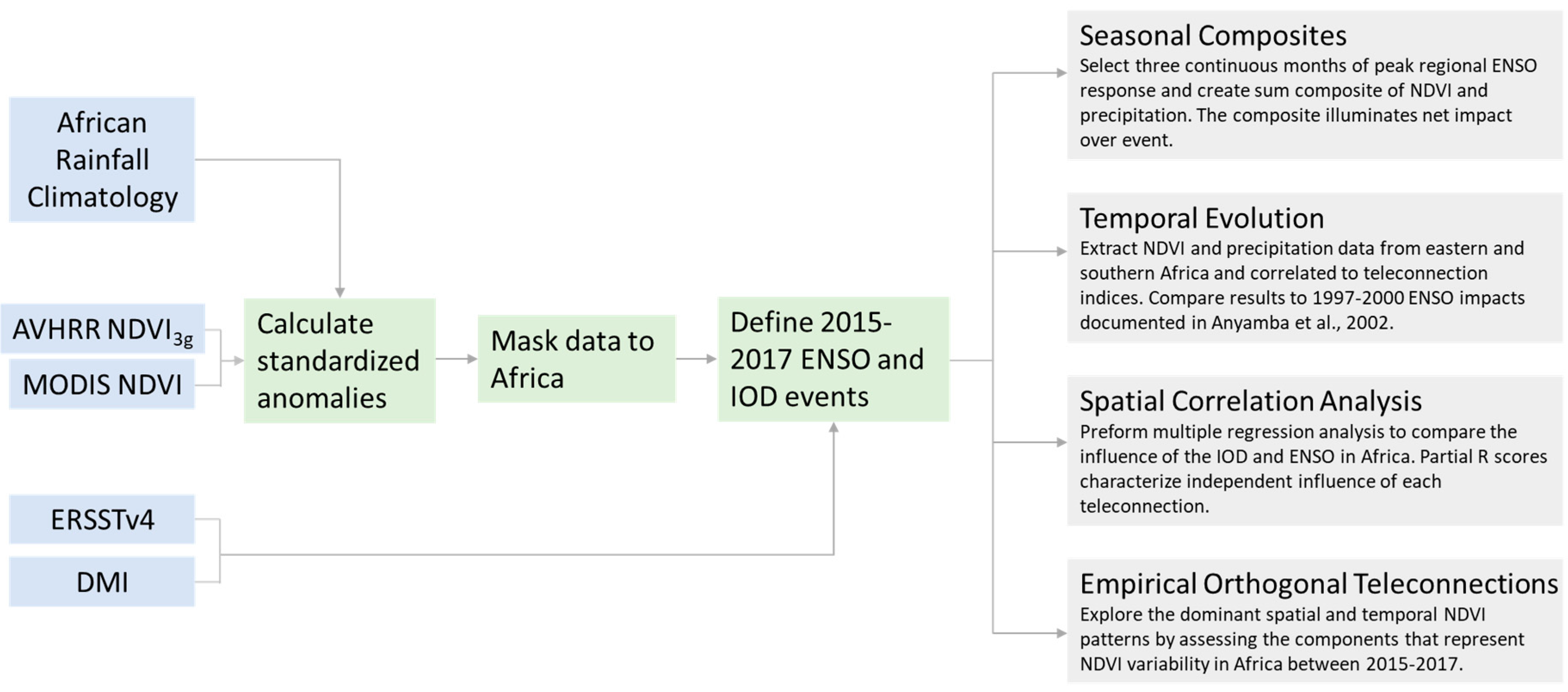
An overview of the methods used in this analysis is presented in Figure 2. Standardized anomalies are used throughout the analysis to isolate the interannual variability in NDVI and precipitation from the seasonal cycle. The standardized anomalies were produced by calculating the climatology, or monthly mean over the entire time series, and standard deviation of each month in the climatology. Next, the anomaly images are created by subtracting the climatology from the original values and dividing by the standard deviation. The result conveys the intensity of the departures relative to the normal range of variability in each pixel. Based on the ONI and the expected annual phase locking of ENSO events [38,39], we selected April 2015 to May 2017 to capture the evolution of the ENSO cycle from the development of El Niño to the end of La Niña. While La Niña, as defined by the ONI, officially ended in December 2016, we continued the analysis through May 2017 to accommodate vegetation response times. Three-month cumulative composites of precipitation and NDVI at peak ENSO conditions illuminate the magnitude and distribution of El Niño and La Niña impacts.
2.2.2. Temporal Evolution of Impacts Analysis
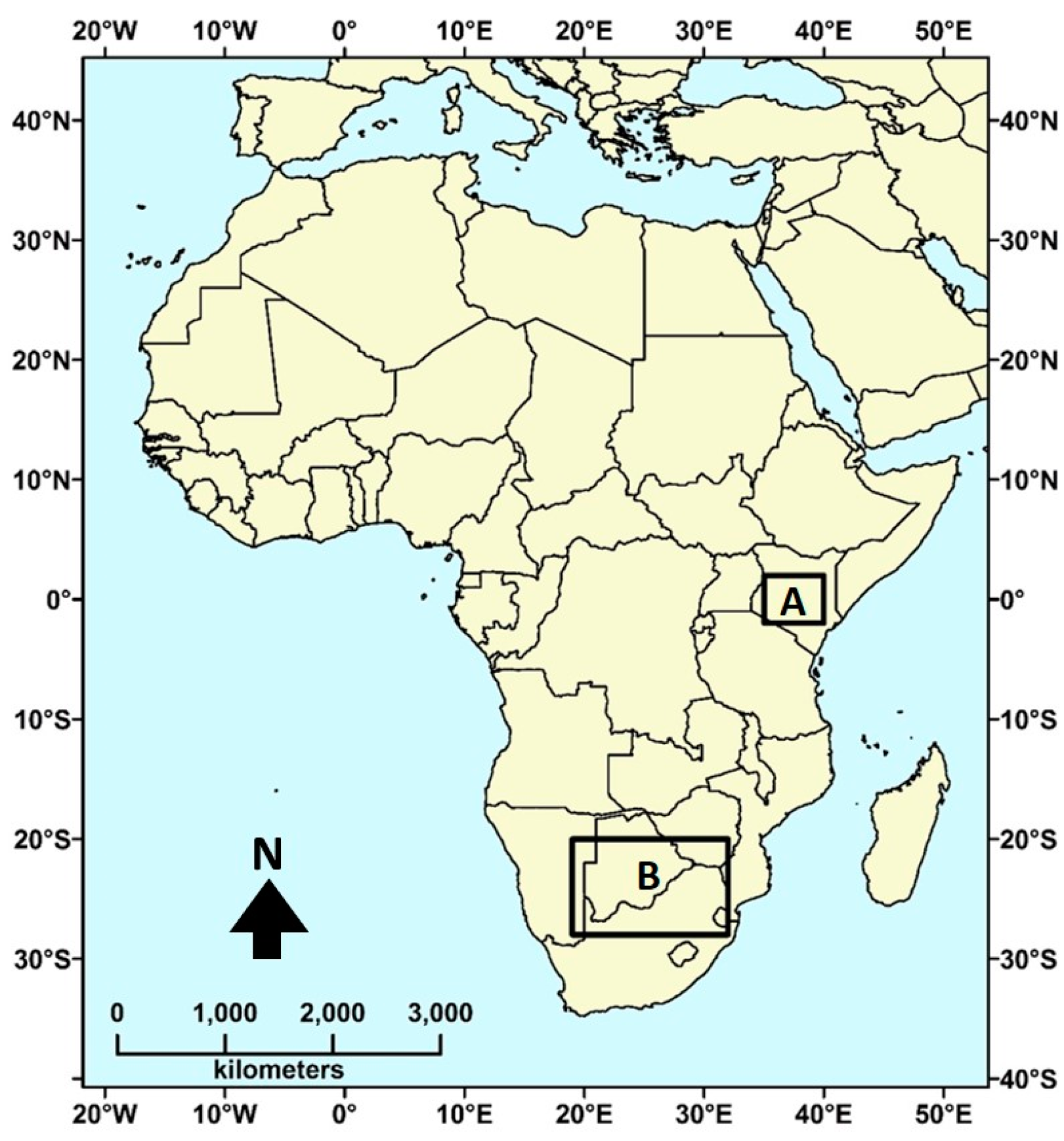
Monthly NDVI and precipitation anomalies were extracted from two agriculture and rangeland regions, one in Kenya and one in South Africa and Botswana (Figure 3). These regions were chosen to match regions defined by Anyamba et al. in 2002 [8] to examine the impacts of the 1997–2000 ENSO, therefore facilitating consistent comparison between the two events. Regression analyses were performed between the regional NDVI and precipitation time series and teleconnection indices. Each regression was run over the course of the 2015–2017 ENSO cycle to assess the immediate correspondence to the SST anomalies. Several lag-time adjustments allowed for determination of the time at which ENSO exerts maximum influence on the rainfall and attendant vegetation.
2.2.3. Spatial Correlation Analysis
A multiple regression was run between NDVI and the two teleconnection indices at multiple lag times to characterize how both ENSO and the IOD impact land surface dynamics in Africa. The R-squared values quantify the NDVI variability explained by the joint teleconnection influence. Partial correlation coefficients isolate the contributions of ENSO and the IOD to vegetation variability in Africa. The NDVI was masked based on a precipitation threshold (lower than 150 mm/year). The correlation statistics are generated on a per pixel basis across the entire continent.
2.2.4. Empirical Orthogonal Teleconnection Analysis
Empirical orthogonal teleconnection (EOT) analysis is a variant of empirical orthogonal functions that is useful for finding patterns that are independent in either time or space [40]. Basic EOT analysis, which is orthogonal in time, was used in this application. The method reduces the time series to representative components by finding locations that explain the maximum variability across the map. Part one of EOT analysis searches for the ‘base point’, or pixel that has the highest combined correlation to all other pixels. Part two removes patterns explained by the base point through linear regression, and then the analysis starts over on the residual data. For each iteration, the outputs are a time series extracted from the base point and a map of the correlation of all pixels to the time series. Using this method, we found that the first and second EOTs were highly correlated with the Niño3.4 and DMI indices, respectively.
3. Results
3.1. Seasonal NDVI and Precipitation Composite Results
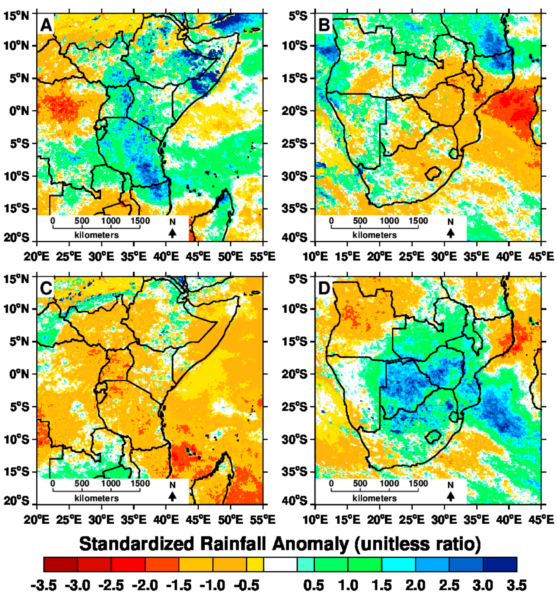
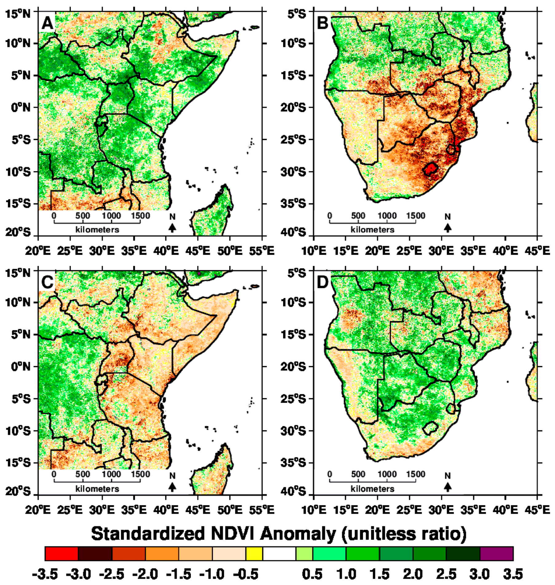
Eastern Africa, particularly Kenya, Uganda, and southcentral Ethiopia had abnormally low precipitation in September and October 2015. As predicted based on past events, positive precipitation and NDVI anomalies became widespread in November and peaked in January. While the direction of the regional response was consistent with the canonical response, the spatial manifestation of the anomalies was rather dispersed. In the canonical El Niño the greatest NDVI and precipitation departures are concentrated in north-east Kenya, south-east Ethiopia, and Somalia (Figure 1). In 2015, the greatest precipitation anomalies shifted westwards to Uganda, south-western Kenya, Tanzania, and the northern border of Mozambique, with isolated in central Somalia and south eastern Ethiopia (Figure 4A). The maximum rainfall departures were in the range of +1.0 to +3.0 standardized deviations (150–400 mm). The NDVI anomalies followed the shift in precipitation, affecting the same regions (Figure 5A). Greener-than-normal conditions continued through April, when vegetation returned to neutral or slightly drier than average.
In 2015, southern Africa exhibited the dry conditions commonly associated with the El Niño phase of the ENSO cycle. Negative NDVI anomalies began to appear in western and central South Africa in September and by November virtually all of the land areas below 15°S were dominated by below-normal precipitation (Figure 4B) and NDVI (Figure 5B). Throughout the event, the dry conditions progressed from west to east across the region, with the largest NDVI departures (~ −2.5 standardized anomalies below average) concentrated over rangeland and agricultural regions in Botswana, Mozambique and eastern South Africa. The precipitation pattern is similar, with maximum departures of −2.0 standardized deviations (~−300 mm) over central Mozambique. By February the drought conditions began to recede; however, the vegetation along the eastern coast was slow to rebound. The drought was mainly concentrated east of 20°E.
In early 2016, dry conditions associated with La Niña developed in eastern Africa and vegetation productivity quickly declined. Widespread negative precipitation and vegetation anomalies persisted from October 2016 through May 2017. The lowest precipitation anomalies of approximately −1.5 standardized anomalies occurred in Kenya, Tanzania, Uganda, and southern Somalia (Figure 4C). Concurrent NDVI has a similar spatial distribution and departures of about −1.0 to −2.0 standardized anomalies below average (Figure 5C).
During the same period, southern Africa experienced enhanced precipitation and vegetation. The strong positive effects may have been a response to the combined influence of the relatively weak La Niña and the warm pool of water in the southern Indian Ocean (Figure 9). The precipitation (Figure 4D) and NDVI (Figure 5D) impacts were particularly strong in Botswana, Zimbabwe, and central and northern South Africa. Maximum precipitation and NDVI departures were both about +2 standardized deviations above average. Although La Niña reached an early peak in October 2016, the NDVI and precipitation anomalies did not fully develop until January to February 2017. The delayed vegetation response may have been due to extended soil moisture recovery time following the extremely dry conditions in the previous year [27,41].
3.2. Temporal Evolution of Impacts Results
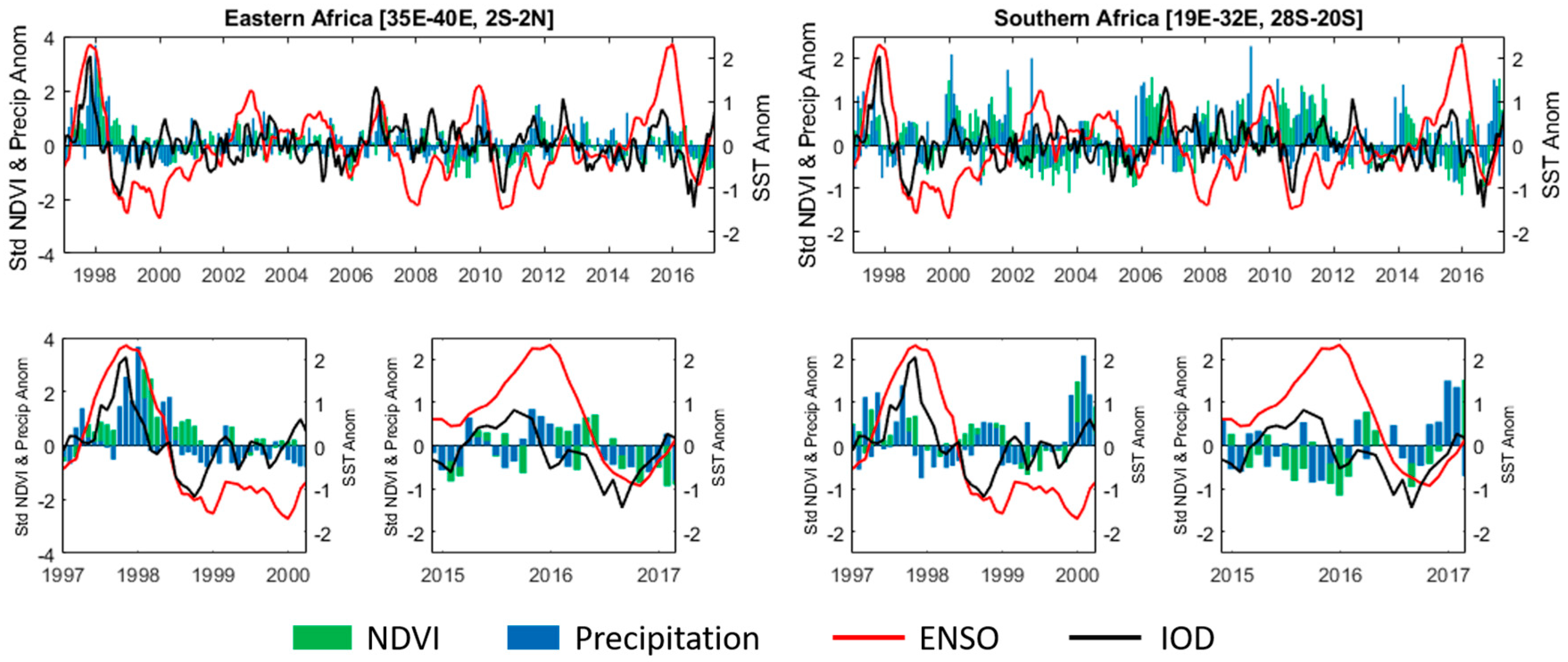
To facilitate comparison between the 1997–2000 ENSO and 2015–2017 ENSO the regions extracted in eastern Africa (35E–40E, 2S–2N) and southern Africa (19E–32E, 28S–20S) correspond to the areas examined in a previous assessment of teleconnection effects in Africa [8]. While patterns described by Anyamba et al. [8] generally align with our observations, there are several differences between the two events. In the 1997–1998 El Niño, eastern Africa more closely reflected the canonical response, with positive extremes concentrated in Kenya and Somalia. NDVI in this region was anomalously high for several months, in contrast to the short and weak green up in this location in November 2015 to February 2016. This is partially explained by the spatial differences in the response patterns; maximum departures were located elsewhere in the later event. As conditions transitioned to La Niña in 1999, NDVI gradually declined and remained slightly below average from September 1999 to February 2001. While the more recent La Niña was a briefer event, the negative NDVI departures were approximately 10–15% greater than the 1999 episode.
Southern Africa presented an atypical response in 1997, which is reflected by the near-normal NDVI throughout most of the event. In fact, we note slightly greener than average vegetation preceding peak El Niño conditions. The 2015 event, however, presented a stronger response with NDVI and precipitation departures of about −1.0 standardized anomaly (Figure 6) in 2015. During La Niña, the maximum NDVI departures of +1.5 standardized anomalies in both 2000 and 2017 occurred in January and in February, respectively.
In both teleconnection regions, the peak precipitation lags the ENSO signal by zero to two months. In eastern Africa, the maximum correlation between ENSO and precipitation (r = 0.56, p < 0.005) occurs without any lag adjustments. The strength of the correlation is stable and significant at lag intervals of up to four months. In southern Africa, the maximum correlation (r = 0.42, p < 0.05) occurs one month after the ENSO signal, and is also significant at two and three months time adjustments. Based on the correlation statistics at several lag times, eastern Africa had a stronger, more immediate precipitation impact than southern Africa in the most recent ENSO event. This is partially due to East Africa’s location within the equatorial plane where ENSO impacts were most pronounced and immediate. The correlation statistics are summarized in Table 1.
Vegetation response to ENSO-induced precipitation anomalies in both regions takes approximately one to two months, and peak correlations occur at a lag of three to four months. The delay may be partially due to growth rates of different vegetation types but more importantly due to mediation between rainfall and vegetation growth via soil moisture [41]. Again, for the 2015–2017 period, ENSO had a stronger influence in eastern Africa than in southern Africa, with correlation coefficients of 0.80 and 0.61, respectively, when NDVI lags ENSO by four months. While the relationship between NDVI and Niño 3.4 is statistically significant at all lag intervals (zero to four months) in eastern Africa, the relationship is only significant for a vegetation lag of three or four months in southern Africa. In both regions, the relationship between NDVI and ENSO is substantially stronger than the relationship between precipitation and ENSO. A possible explanation for the difference is due to the randomness or day-to-day variability in rainfall over the season compared to the relatively stable and gradual growth or decline in vegetation over space and time.
3.3. Spatial Correlation Results
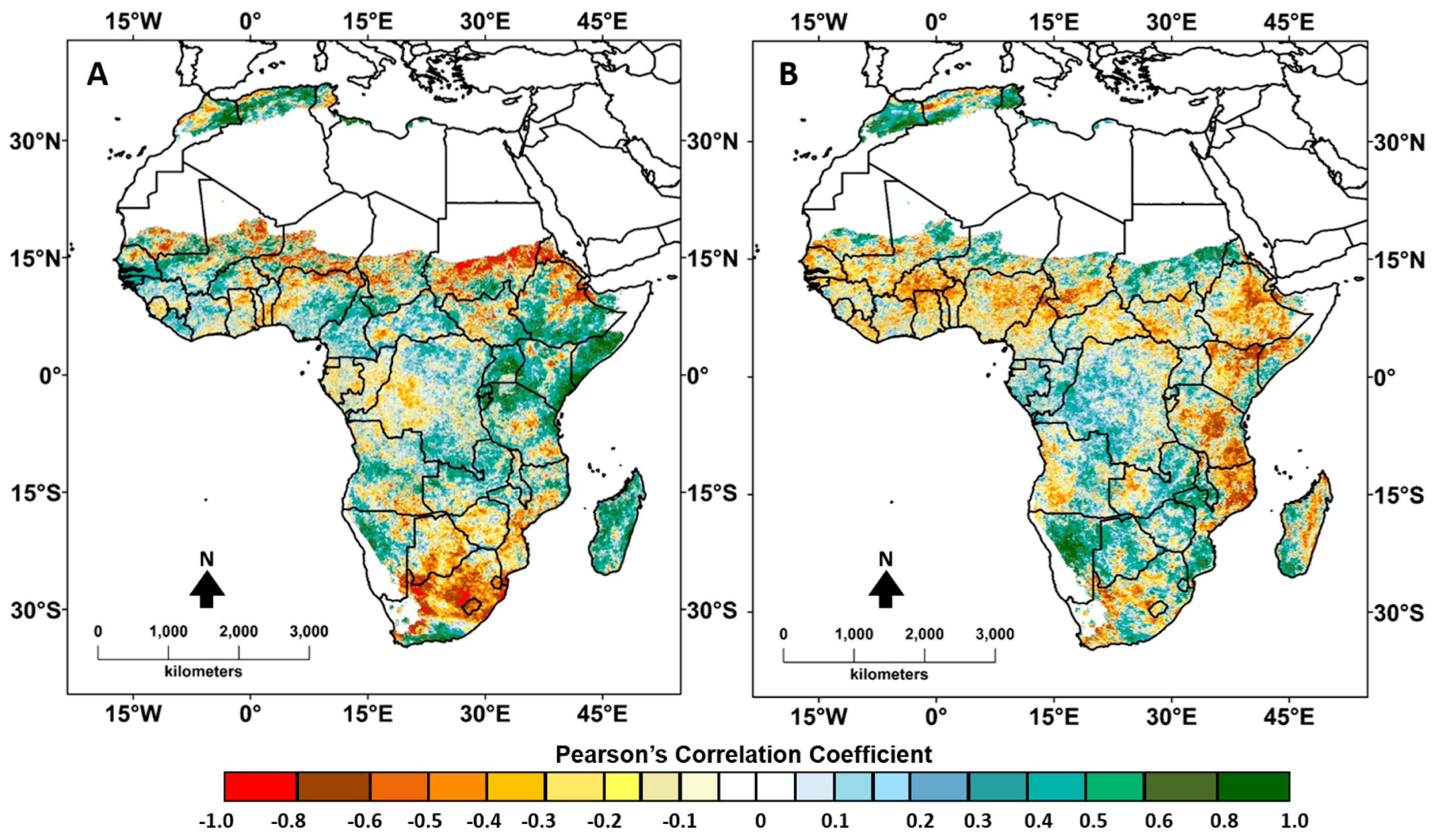
The multiple regression between Niño 3.4, the DMI, and NDVI in Africa illuminated the independent impacts of each teleconnection on land surface dynamics in Africa (Figure 7). In the partial correlation maps the green values indicate that the time-series of NDVI values at the pixel is positively correlated to Niño 3.4 (right) or the DMI (left). Red pixels indicate a negative relationship.
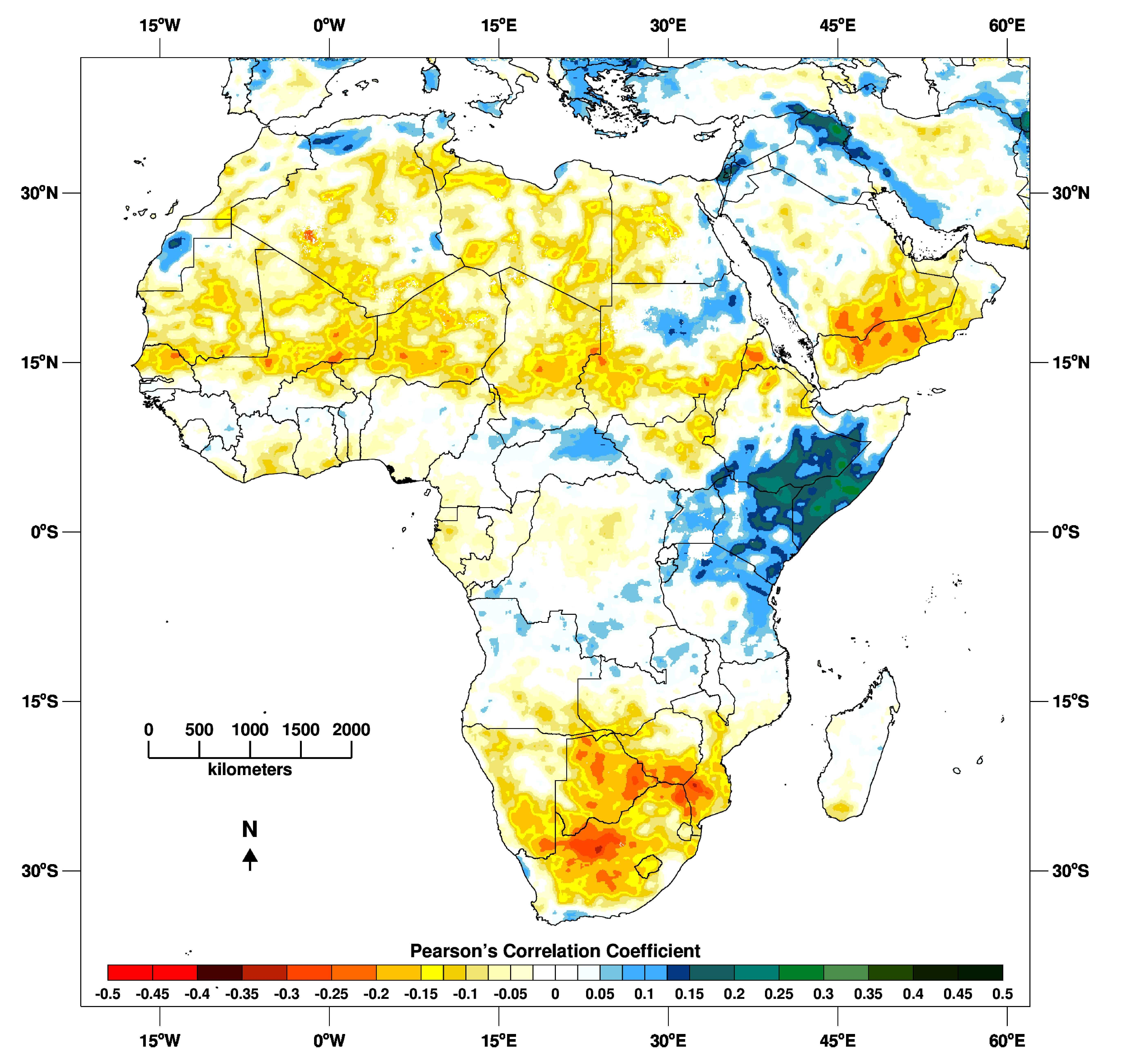
As expected, Niño 3.4 was associated with a strong dipole pattern. This confirms that eastern African vegetation was positively correlated to ENSO in the 2015–2017 event and, therefore, has higher (lower) vegetation productivity in El Niño (La Niña). Although the coast of Kenya did not experience major vegetation impacts in the 2015–2017 event, the strong positive relationship apparent in the correlation analysis indicates the cycle was in sync even though the amplitude of the effect was not large. We see that the opposite pattern characterizes the response in southern Africa. However, in South Africa, we find an exception to the general pattern along the southern coast (Cape region). This ecologically and climatologically distinct region had a strong negative association with El Niño, which may be related to underlying differences in local topography and regional ocean influence [42].
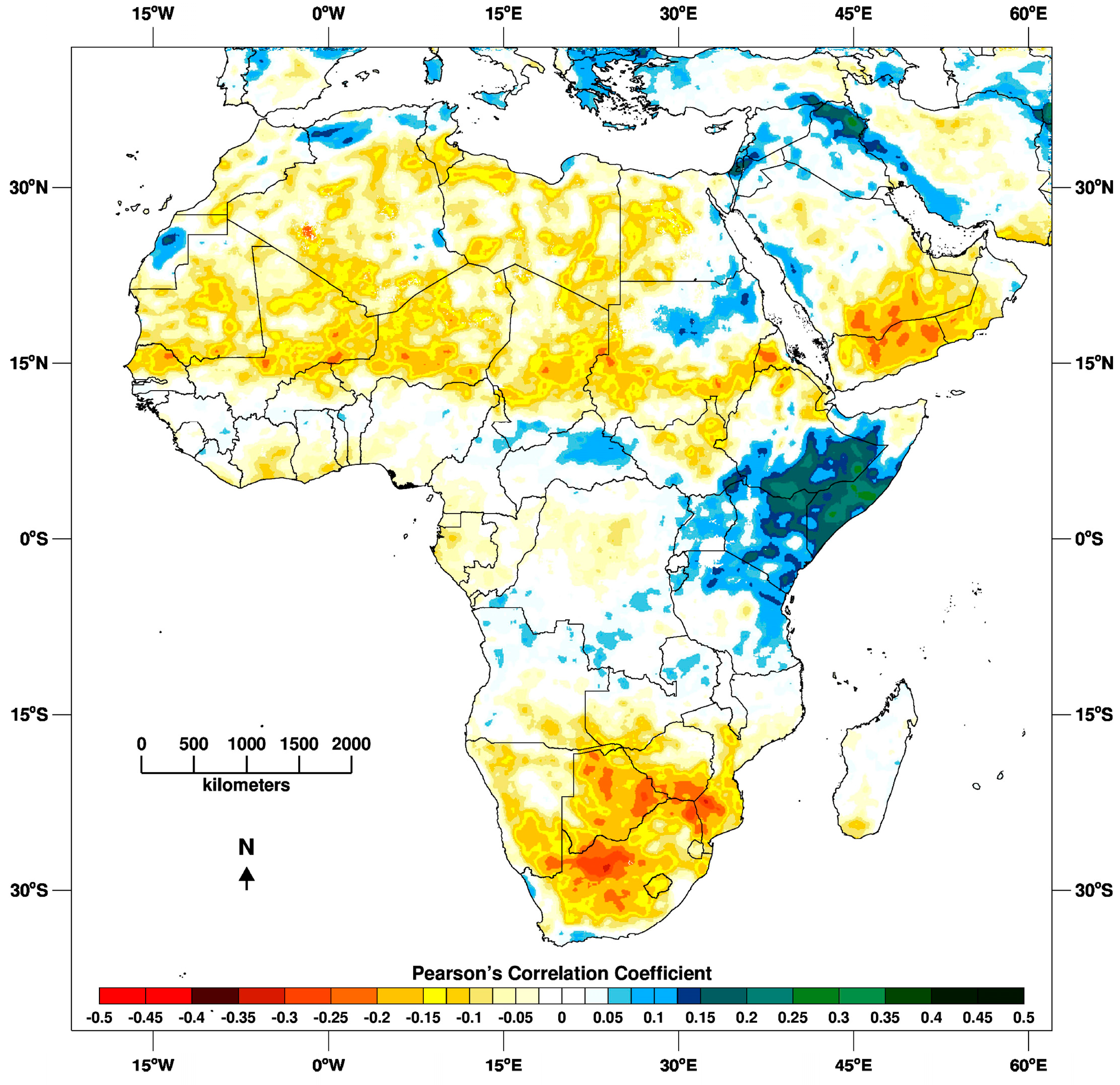
The correlation between NDVI and the DMI presents a less cohesive spatial pattern. While eastern Africa generally has enhanced precipitation associated with the IOD, we see the region is dominated by a negative relationship. Instead, the positive impact migrated south to Zimbabwe and southern Mozambique. This pattern reflects the basin-wide warming that occurred in the Indian Ocean during the El Niño, and concentrated warm SST anomalies off the coast of southern Africa during the La Niña (Figure 9).
The highest R2 values are concentrated in southern Africa and eastern Africa, indicating that changes in eastern tropical Pacific Ocean SSTs explain a substantial amount of vegetation variability in these regions. Specifically, ENSO is most closely related to South Africa (particularly the east and along the southern coast), Somalia, eastern Ethiopia, and south-east Kenya. During this period, the IOD had the strongest influence on Botswana, Zambia, and Zimbabwe. This finding was rather unexpected but may be attributed to the basin-wide warming within the entire Indian Ocean.
3.4. Empirical Orthogonal Teleconnections (EOT) Results
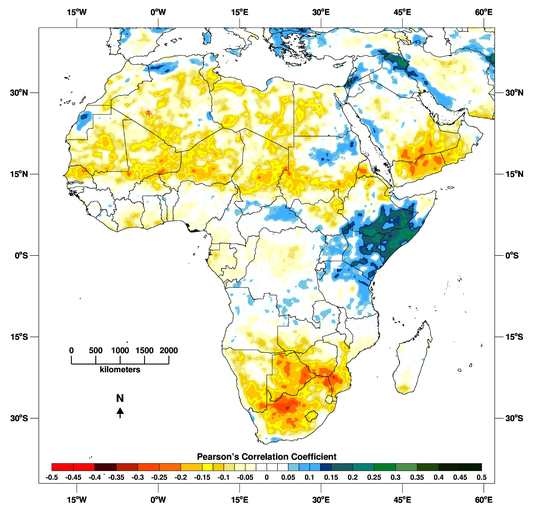
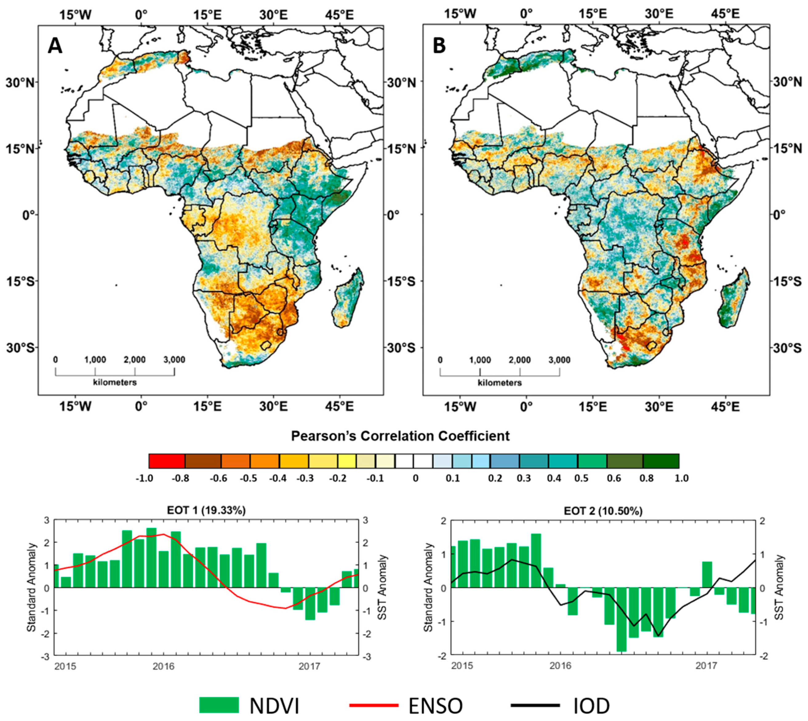
The EOT analysis successfully distinguished the impacts of ENSO and the IOD on NDVI in Africa. The first EOT, which represents 19.33% of the NDVI variability, clearly corresponds to ENSO (r = 0.60, p < 0.05) (Figure 8A). The locus of this relationship was centered at a location in Somalia which is highly correlated to other pixels. When this time series is correlated to all other pixels, the dipole pattern between eastern and southern Africa emerges and is very similar to the canonical pattern shown in Figure 1.
The second EOT result, selected from a location in western Madagascar, was strongly correlated to all other pixels after the influence of the first EOT was removed. The EOT 2 represents 10.50% of the NDVI variability and is correlated to the IOD signal (r = 0.70, p < 0.05). The trend shows less of a lag effect than the NDVI pattern associated with ENSO, perhaps due to the proximity of the Indian Ocean. The correlation between each pixel and the trend presents a similar pattern to that found in the spatial correlation analysis (Figure 8B). However, in the EOT 2 result the negative impacts are concentrated in central and southern Tanzania, northern Mozambique, and central South Africa. The eastern coast of Kenya and Madagascar show a more positive effect than in the spatial correlation result. Overall, this pattern is rather diffuse and not spatially coherent.
4. Discussion
The interannual variability in the coupled ocean atmosphere system has impacts on the land surface revealed through coherent and persistent departures in rainfall and vegetation. More importantly, this translates into significant social economic impacts. During the 2015–2017 ENSO such impacts are evident in the agricultural production records for eastern and southern Africa [43]. Corn yields in Kenya were 17% above average in 2015 due to the favorable precipitation conditions associated with El Niño [44]. The following growing seasons in 2016 and 2017, however, were extremely dry. Low crop production, coupled with high food prices and heavy livestock losses led to acute food insecurity, disease outbreaks, and conflict across the region [45]. South Africa faced dry conditions in the 2014–2015 season, which exacerbated the drought brought by El Niño in 2015–2016. Although irrigated corn area has more than doubled between 2000 and 2013, water stress led to planting delays and subsequent reductions in corn crop area and production, with a total yield of 8.4 million metric tons [46]. Fortunately, the La Niña-induced rain during the 2016–2017 growing season mitigated the drought. The favorable weather conditions resulted in a record-breaking corn crop of 16.4 million metric tons, doubling that of the previous season [46].
Past research has identified a similar reversal in vegetation response patterns between El Niño and La Niña in both eastern and southern Africa [8,9,10]. Parhi et al. [10] focus on tropical Africa, and characterize modulations in tropical African rainfall in response to the growth and mature phases of El Niño. They find that impacts in eastern Africa are most intense during the short rainy season (October–December) and manifest as changes in frequency, rather than intensity, of precipitation. In an analysis of 30 years of NDVI data, Philippon et al. [9] find that relative to other regions in Africa, eastern and southern Africa have the highest percentage of pixels significantly related to ENSO and the highest overall correlation values. Interestingly, they divide eastern Africa into two regions with distinct ENSO impacts: northern eastern Africa, which has a negative correlation with ENSO during the summer rainfall season, and equatorial eastern Africa, which presents a strong positive correlation.
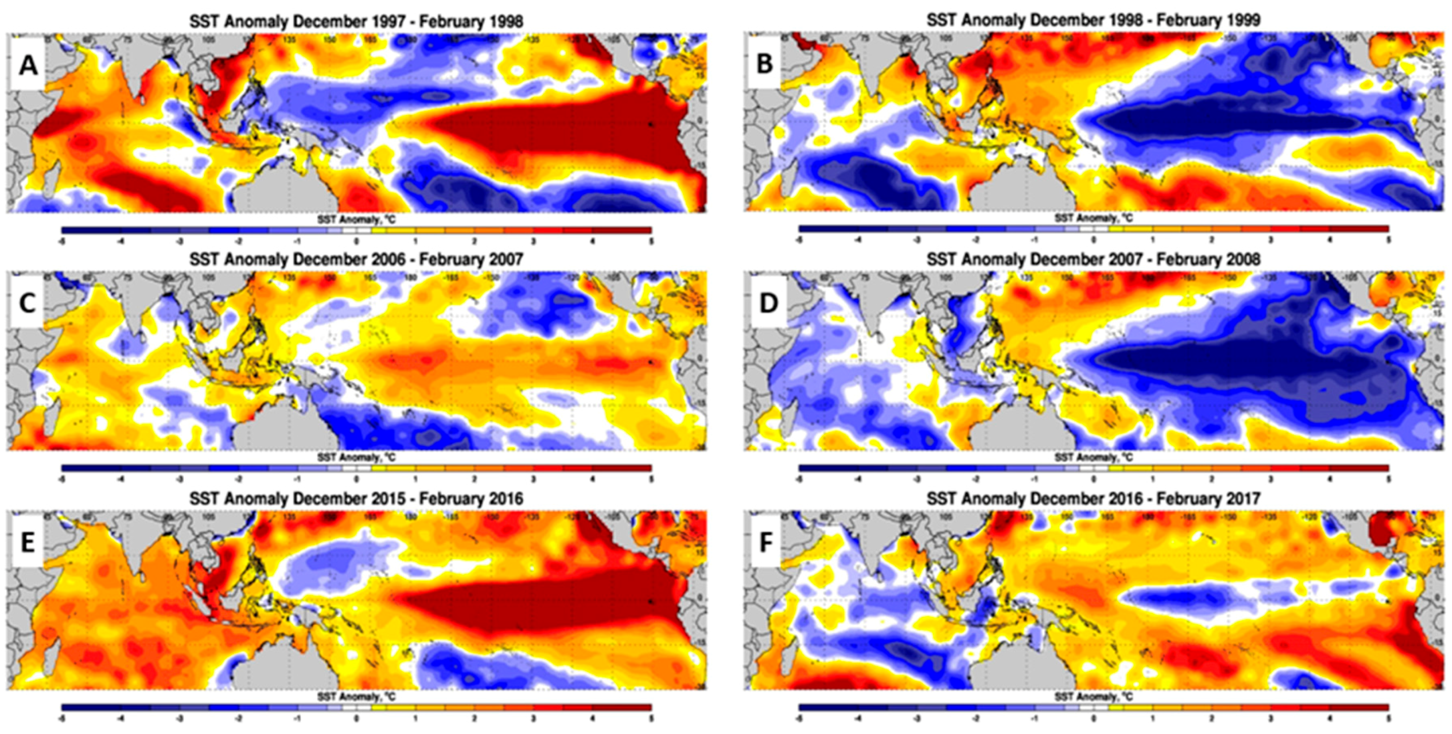
Indian Ocean SSTs are a critical factor governing climate variability in Africa and play a role in the outcome of ENSO events. The IOD was positive preceding peak El Niño conditions from November to January 2015, when it returned to a neutral state. Although the DMI suggests there was a dipole pattern, we observe that the entire Indian Ocean basin was warm from December 2015 to February 2016 (Figure 9). Furthermore, the warm SST anomalies were not concentrated along the equator and close to the coast of eastern Africa as in the case of the 1997–1998 El Niño, and the spatial pattern was diffuse overall. Compared to the strong IOD in December 1997 to February 1998, the weak spatial structure of the latest IOD is especially striking. We hypothesize that the El Niño event enhanced SSTs across the Indian Ocean basin, but the sporadic manifestation of warm anomalies resulted in the south-west shift of effects in eastern Africa. We note that warm SST anomalies in the southern Indian Ocean in December 2016 to February 2017 likely amplified the La Niña effects in southern Africa. While these events provide some insight into how SST anomalies influence African precipitation and vegetation, analysis of a longer time period is necessary to better understand the interactions between ENSO and the IOD and predict the outcomes.
The eastern or central position of SST anomalies in the Pacific Ocean basin is another critical factor in ENSO dynamics [47]. Although it is unclear whether the two types are mechanistically distinct or two manifestations of non-linear ENSO properties [48,49], the placement has implications for the timing, teleconnections, and Indian Ocean interaction [50]. Eastern Pacific (EP) ENSO events are considered the ‘canonical’ type and are more likely to result in strong impacts. The SSTs are concentrated along the South American coast and extend into the equatorial Pacific, driving basin-wide thermocline and surface wind oscillations. Alternately, Central Pacific (CP) ENSO events occur when the surface wind and SST anomalies are confined to the central Pacific, reducing the strength of teleconnection effects [50].
Interestingly, the 2015–2016 El Niño had characteristics of CP and EP events and is not easily classified as either. Warm SSTs were concentrated in the central Pacific to the western coast of South and Central America, where the warm water spreads north and south along the coast (Figure 9). Although the warmest water was located in the central/eastern Pacific, rather than along the South American coast, there was a clear basin-wide effect. In general, the widespread shift in ocean temperature generated the expected teleconnection effects in Africa. Although the La Niña was weak and had a small SST footprint, we still observe the known vegetation and precipitation effects.
5. Conclusions
The 2015–2017 ENSO episode clearly influenced climate and land surface response patterns in eastern and southern Africa. The impacts are evident in the precipitation, NDVI, and agricultural production records. Our results confirm that both regions are significantly correlated with equatorial Pacific SSTs and exhibit a clear dipole pattern that reverses between warm and cold ENSO events. Interestingly, precipitation—the variable most directly connected to global atmospheric and oceanic oscillations—had the weakest overall correlation to the teleconnection indices. The ENSO signal, with contributions from the IOD, more clearly influenced NDVI and the ultimate agricultural outcomes. The time-scale of vegetation responses, a process of biophysical changes in the plant, may be more in sync with the gradual fluctuations in SSTs associated with ENSO and IOD events than the relative randomness of precipitation over space and time. We suggest that NDVI can continue to be used as an integral part of the evaluation of ENSO impacts in Africa and similar semi-arid lands globally.
While the familiar canonical patterns were observed, we find variations in the placement and magnitude of the precipitation and vegetation anomalies in the latest event. The greatest impacts in eastern Africa migrated westward and southward of the usual position and of the 1997–2000 event, and the positive La Niña impact in South Africa was especially strong. These subtle shifts are likely due to the specific properties of SST anomalies in the Pacific basin and interactions with Indian Ocean SST anomalies; however, attributing these observations to forces driving ENSO variations is outside of the scope of the current work.
Several analytical techniques facilitated our exploration of the ENSO teleconnection effects, each with its own strengths and limitations. The seasonal composites provide an intuitive and informative snapshot of NDVI and precipitation conditions, but do not provide insight into the drivers of the observations. Time series correlation analysis demonstrates the magnitude and timing of correspondence between Niño 3.4, the DMI, precipitation, and NDVI. However, the regionally averaged signal used in the comparison obscures local patterns. Spatial correlation analysis fills this gap, and illuminates locations where the local pattern either agrees with, or differs from, the regional trend. EOT analysis distills the time series into the most representative patterns, specifically designed to investigate teleconnection impacts. However, the method is computationally intensive and yielded similar results to the spatial correlation analysis.
Together the analyses are very useful for documenting the effects of ENSO and the IOD, which provides insight into variability in the teleconnections and informs future predictions. Additionally, well-documented effects can inform targeted mitigation and relief efforts, such as altering planting practices, formulating insurance coverages, planning emergency food assistance, and vaccinating animals. The availability of an 18-year MODIS time-series record provides opportunities to employ different analysis techniques, such as those used in this analysis, that are easily repeatable and could be used as a guideline for consistent monitoring. Our analysis and results show that the manifestations of ENSO and IOD impacts on the land surface can depart from the canonical pattern, and therefore it is critical to continue monitoring and documenting rainfall and vegetation extremes associated with ENSO and IOD events.
Author Contributions
Conceptualization, A.A.; Methodology, A.A. and E.G.; Validation, A.A., E.G., and J.S.; Formal Analysis, E.G.; Investigation, E.G.; Resources, A.A.; Data Curation, E.G.; Writing-Original Draft Preparation, E.G.; Writing-Review & Editing, A.A. and E.G.; Visualization, E.G. and J.S.; Supervision, A.A.; Project Administration, A.A.; Funding Acquisition, A.A.
Funding
This research is supported by the United States Department of Agriculture Foreign Agricultural Service in support of the Global Agriculture Monitoring system (ttps://glam1.gsfc.nasa.gov/).
Conflicts of Interest
The authors declare no conflicts of interest.
References
- McPhaden, M.J.; Zebiak, S.E.; Glantz, M.H. ENSO as an Integrating Concept in Earth Science. Science 2006, 314, 1740–1745. [Google Scholar] [CrossRef] [PubMed]
- David Neelin, J.; Latif, M. El Niño Dynamics. Phys. Today 1998, 51, 32–36. [Google Scholar] [CrossRef] [Green Version]
- Trenberth, K.E. The Definition of El Niño. Bull. Am. Meteorol. Soc. 1997, 78, 2771–2777. [Google Scholar] [CrossRef] [Green Version]
- Ropelewski, C.; Halpert, M.S. Global and Regional Scale Precipitation Patterns Associated with the El Niño/Southern Oscillation. Mon. Weather Rev. 1987, 115, 1606–1626. [Google Scholar] [CrossRef] [Green Version]
- Myneni, R.B.; Los, S.O.; Tucker, C.J. Satellite-based identifiction of linked vegetation index and sea surface temperature anomaly areas from 1982–1990 for Africa, Australia, and South America. Geophys. Res. Lett. 1996, 23, 729–732. [Google Scholar] [CrossRef]
- Anyamba, A.; Eastman, J.R. Interannual variability of NDVI over Africa and its relation to El Niño/Southern Oscillation. Int. J. Remote Sens. 1996, 17, 2533–2548. [Google Scholar] [CrossRef]
- Nicholson, S.E.; Kim, J. The Relationship of the El Niño–Southern Oscillation To African Rainfall. Int. J. Climatol. 1997, 17, 117–135. [Google Scholar] [CrossRef]
- Anyamba, A.; Tucker, C.J.; Mahoney, R. From El Niño to La Niña: Vegetation response patterns over east and southern Africa during the 1997–2000 period. J. Clim. 2002, 15, 3096–3103. [Google Scholar] [CrossRef]
- Philippon, N.; Martiny, N.; Camberlin, P.; Hoffman, M.T.; Gond, V. Timing and patterns of the ENSO signal in Africa over the last 30 years: Insights from Normalized Difference Vegetation Index Data. J. Clim. 2014, 27, 2509–2532. [Google Scholar] [CrossRef]
- Parhi, P.; Giannini, A.; Gentine, P.; Lall, U. Resolving contrasting regional rainfall responses to EL Niño over tropical Africa. J. Clim. 2016, 29, 1461–1476. [Google Scholar] [CrossRef]
- Martiny, N.; Richard, Y.; Camberlin, P. Interannual persistence effects in vegetation dynamics of semi-arid Africa. Geophys. Res. Lett. 2005, 32, 1–4. [Google Scholar] [CrossRef]
- Birkett, C.; Murtugudde, R.; Allan, T. Indian Ocean climate event brings floods to East Africa’s lakes and the Sudd marsh. Geophys. Res. Lett. 1999, 26, 1031–1034. [Google Scholar] [CrossRef]
- Williams, C.; Hanan, N.P. ENSO and IOD teleconnections for African ecosystems: Evidence of destructive interference between climate oscillations. Biogeosciences 2011, 8, 27–40. [Google Scholar] [CrossRef] [Green Version]
- Saji, H.N.; Goswami, B.N.; Vinayachandran, P.N.; Yamagata, T. A dipole mode in the tropical Indian Ocean. Nature 1999, 401, 360–363. [Google Scholar] [CrossRef] [PubMed]
- Webster, P.J.; Moore, A.M.; Loschnigg, J.P.; Leben, R.R. Coupled ocean–atmosphere dynamics in the Indian Ocean during 1997–98. Nature 1999, 401, 356–360. [Google Scholar] [CrossRef] [PubMed]
- Yamagata, T.; Behera, S.K.; Rao, S.A.; Guan, Z.; Ashok, K.; Saji, H.N. Comments on “Dipoles, Temperature Gradients, and Tropical Climate Anomalies.”. Bull. Am. Meteorol. Soc. 2003, 84, 1418–1422. [Google Scholar] [CrossRef]
- Ashok, K.; Guan, Z.; Yamagata, T. A Look at the Relationship between the ENSO and the Indian Ocean Dipole. J. Meteorol. Soc. Jpn. 2003, 81, 41–56. [Google Scholar] [CrossRef]
- Behera, S.K.; Luo, J.J.; Masson, S.; Rao, S.A.; Sakuma, H.; Yamagata, T. A CGCM study on the interaction between IOD and ENSO. J. Clim. 2006, 19, 1688–1705. [Google Scholar] [CrossRef]
- Dommenget, D. An objective analysis of the observed spatial structure of the tropical Indian Ocean SST variability. Clim. Dyn. 2011, 36, 2129–2145. [Google Scholar] [CrossRef]
- Zhao, Y.; Nigam, S. The Indian ocean dipole: A monopole in SST. J. Clim. 2015, 28, 3–19. [Google Scholar] [CrossRef]
- Black, E. The relationship between Indian Ocean sea-surface temperature and East African rainfall. Philos. Trans. A. Math. Phys. Eng. Sci. 2005, 363, 43–47. [Google Scholar] [CrossRef] [PubMed]
- Jiménez-Muñoz, J.C.; Mattar, C.; Barichivich, J.; Santamaría-Artigas, A.; Takahashi, K.; Malhi, Y.; Sobrino, J.A.; Schrier, G. van der Record-breaking warming and extreme drought in the Amazon rainforest during the course of El Niño 2015–2016. Sci. Rep. 2016, 6, 33130. [Google Scholar] [CrossRef] [PubMed]
- Field, R.D.; van der Werf, G.R.; Fanin, T.; Fetzer, E.J.; Fuller, R.; Jethva, H.; Levy, R.; Livesey, N.J.; Luo, M.; Torres, O.; et al. Indonesian fire activity and smoke pollution in 2015 show persistent nonlinear sensitivity to El Niño-induced drought. Proc. Natl. Acad. Sci. USA 2016, 113, 9204–9209. [Google Scholar] [CrossRef] [PubMed]
- Stige, L.C.; Stave, J.; Chan, K.-S.; Ciannelli, L.; Pettorelli, N.; Glantz, M.; Herren, H.R.; Stenseth, N.C. The effect of climate variation on agro-pastoral production in Africa. Proc. Natl. Acad. Sci. USA 2006, 103, 3049–3053. [Google Scholar] [CrossRef] [PubMed] [Green Version]
- Nicholson, S.E.; Davenport, M.L.; Malo, A.R. A comparison of the vegetation response to rainfall in the Sahel and East Africa, using normalized difference vegetation index from NOAA AVHRR. Clim. Chang. 1990, 17, 209–241. [Google Scholar] [CrossRef]
- Ichii, K.; Kawabata, A.; Yamaguchi, Y. Global correlation analysis for NDVI and climatic variables and NDVI trends: 1982–1990. Int. J. Remote Sens. 2002, 23, 3873–3878. [Google Scholar] [CrossRef]
- Martiny, N.; Camberlin, P.; Richard, Y.; Philippon, N. Compared regimes of NDVI and rainfall in semi-arid regions of Africa. Int. J. Remote Sens. 2006, 27, 5201–5223. [Google Scholar] [CrossRef]
- Richard, Y.; Poccard, I. A statistical study of NDVI sensitivity to seasonal and interannual rainfall variations in Southern Africa. Int. J. Remote Sens. 1998, 19, 2907–2920. [Google Scholar] [CrossRef]
- Andujar, E.; Krakauer, N.Y.; Yi, C.; Kogan, F. Ecosystem Drought Response Timescales from Thermal Emission Versus Shortwave Remote Sensing. Adv. Meteorol. 2017, 2017, 1–29. [Google Scholar] [CrossRef]
- Zhang, X.; Zhang, Q. Monitoring interannual variation in global crop yield using long-term AVHRR and MODIS observations. ISPRS J. Photogramm. Remote Sens. 2016, 114, 191–205. [Google Scholar] [CrossRef]
- Glennie, E.; Anyamba, A. Midwest agriculture and ENSO: A comparison of AVHRR NDVI3g data and crop yields in the United States Corn Belt from 1982 to 2014. Int. J. Appl. Earth Obs. Geoinf. 2018, 68, 180–188. [Google Scholar] [CrossRef]
- Didan, K.; Munoz, A.B.; Huete, A. MODIS Vegetation Index User’s Guide (MOD13 Series); VIP Research Group, The University of Arizona: Tucson, AZ, USA, 2015; Volume 3. [Google Scholar]
- Pinzon, J.E.; Tucker, C.J. A non-stationary 1981–2012 AVHRR NDVI3g time series. Remote Sens. 2014, 6, 6929–6960. [Google Scholar] [CrossRef]
- Love, T.B.; Kumar, V.; Xie, P.-P.; Thiaw, W.M. A 20-year daily Africa precipitation climatology using satellite and gauge data. In Proceedings of the 84th American Meteorological Society Annual Meeting, Seattle, WA, USA, 11–15 January 2004; pp. 5213–5216. [Google Scholar]
- Novella, N.S.; Thiaw, W.M. A seasonal rainfall performance probability tool for famine early warning systems. J. Appl. Meteorol. Climatol. 2016, 55, 2575–2586. [Google Scholar] [CrossRef]
- Huang, B.; Banzon, V.F.; Freeman, E.; Lawrimore, J.; Liu, W.; Peterson, T.C.; Smith, T.M.; Thorne, P.W.; Woodruff, S.D.; Zhang, H.M. Extended reconstructed sea surface temperature version 4 (ERSST.v4). Part I: Upgrades and intercomparisons. J. Clim. 2015, 28, 911–930. [Google Scholar] [CrossRef]
- Japan Agency for Marine-Earth Science and Technology Indian Ocean Dipole Mode Index (DMI). Available online: http://www.jamstec.go.jp/frcgc/research/d1/iod/HTML/Dipole Mode Index.html (accessed on 1 September 2017).
- Rasmusson, E.M.; Carpenter, T.H. Variations in Tropical Sea Surface Temperature and Surface Wind Fields Associated with the Southern Oscillation/El Niño. Mon. Weather Rev. 1982, 110, 354–384. [Google Scholar] [CrossRef] [Green Version]
- Rasmusson, E.M.; Wang, X.; Ropelewski, C.F. The biennial component of ENSO variability. J. Mar. Syst. 1990, 1, 71–96. [Google Scholar] [CrossRef]
- Van Den Dool, H.M.; Saha, S.; Johansson, Å. Empirical orthogonal teleconnections. J. Clim. 2000, 13, 1421–1435. [Google Scholar] [CrossRef]
- Mladenova, I.E.; Bolten, J.D.; Crow, W.T.; Anderson, M.C.; Hain, C.R.; Johnson, D.M.; Mueller, R. Intercomparison of Soil Moisture, Evaporative Stress, and Vegetation Indices for Estimating Corn and Soybean Yields over the U.S. IEEE J. Sel. Top. Appl. Earth Obs. Remote Sens. 2017, 10, 1328–1343. [Google Scholar] [CrossRef]
- Singleton, A.T.; Reason, C.J.C. Numerical simulations of a severe rainfall event over the Eastern Cape coast of South Africa: Sensitivity to sea surface temperature and topography. Tellus Ser. A Dyn. Meteorol. Oceanogr. 2006, 58, 355–367. [Google Scholar] [CrossRef]
- FAOSTAT. FAO Statistical Databases. Food and Agriculture; FAOSTAT: Rome, Italy, 2017. [Google Scholar]
- Kenya Grain and Feed Annual 2016 Kenya Corn, Wheat and Rice Report. Available online: http://gain.fas.usda.gov/Recent GAIN Publications/Grain and Feed Annual_Nairobi_Kenya_4-8-2014.pdf (accessed on 1 December 2017).
- Global Alert: Very Large Assistance Needs and Famine Risk Will Continue in 2018. Available online: http://www.fews.net/print/global/alert/november-28-2017 (accessed on 1 December 2017).
- Office of Global Analysis of Production Briefs, Crop Explorer Production Briefs—Southern Africa. Available online: https://ipad.fas.usda.gov/cropexplorer/pecad_stories.aspx?regionid=safrica&ftype=prodbriefs (accessed on 15 January 2018).
- Yeh, S.W.; Kug, J.S.; An, S. Il Recent progress on two types of El Niño: Observations, dynamics, and future changes. Asia-Pac. J. Atmos. Sci. 2014, 50, 69–81. [Google Scholar] [CrossRef]
- Takahashi, K.; Montecinos, A.; Goubanova, K.; Dewitte, B. ENSO regimes: Reinterpreting the canonical and Modoki El Niño. Geophys. Res. Lett. 2011, 38, 1–5. [Google Scholar] [CrossRef]
- Jeong, H.I.; Ahn, J.B. A new method to classify ENSO events into eastern and central Pacific types. Int. J. Climatol. 2017, 37, 2193–2199. [Google Scholar] [CrossRef]
- Kao, H.Y.; Yu, J.Y. Contrasting Eastern-Pacific and Central-Pacific types of ENSO. J. Clim. 2009, 22, 615–632. [Google Scholar] [CrossRef]
Figure 1.
The map shows the ‘canonical’ vegetation response patterns associated with the El Niño Southern Oscillation (ENSO), derived by correlating Niño 3.4 SST index with monthly anomalies of AVHRR NDVI3g data from 1981 to 2017. The result shows a dipole pattern in vegetation response between eastern Africa (+) and southern Africa (−).

Figure 2.
Flowchart of data and methods used in this analysis.

Figure 3.
Precipitation and normalized difference vegetation index (NDVI) data were extracted in East Africa between 35E–40E and 2S–2N(A) and South Africa between 19E–32E and 28S–20S(B), and analyzed with respect to the sea surface temperature (SST) anomalies in the Niño 3.4 region of the Pacific to assess the coherence, timing, and intensity of teleconnection effects.

Figure 4.
Standardized seasonal precipitation anomalies at peak El Niño conditions in (A) eastern Africa from November 2015 to January 2016; and (B) southern Africa from December 2015 to February 2016. Precipitation anomalies during peak La Niña conditions are displayed in (C) eastern Africa from November 2016 to January 2017 in and (D) in southern Africa from December 2016 to February 2017.

Figure 5.
Standardized seasonal NDVI anomalies at peak El Niño conditions in (A) eastern Africa from November 2015 to January 2016; and (B) southern Africa from December 2015 to February 2016. NDVI anomalies during peak La Niña conditions are displayed in (C) eastern Africa from November 2016 to January 2017 in and (D) in southern Africa from December 2016 to February 2017.

Figure 6.
NDVI (green), precipitation (blue), Niño 3.4 (red line), and the dipole mode index (DMI) (black line) are compared from January 1997 to May 2017 in eastern Africa (35E–40E, 2S–2N) and southern Africa (19E–32E, 28S–20S) in the top figures. Below, the time series from 1997–2000 and 2015–2017 ENSO cycles are extracted to show the patterns in greater detail.

Figure 7.
The maps above show the partial correlation coefficients between teleconnection indices and standardized NDVI anomalies from April 2015 to May 2017. (A) Shows the correlation between the ENSO and vegetation anomalies; and (B) shows the correlation between the Indian Ocean Dipole (IOD) vegetation anomalies, when the IOD precedes the NDVI anomalies by three months.

Figure 8.
Figures A and B represent the first and second results of the empirical orthogonal teleconnections (EOT) analysis, respectively. In figure A, the NDVI pattern captured in EOT 1 and the ENSO signal are compared in the time series plot and the spatial correlation of pixels to the trend is represented in the map. Figure B displays the time series plot and correlation map for EOT 2, which corresponds to the IOD signal.

Figure 9.
Cumulative SST anomalies in the Pacific and Indian Ocean basins during three ENSO events. (A) shows the distinct ‘warm tongue’ pattern that formed in the 1997 El Niño and corresponding dipole in the Indian Ocean; and (B) shows the reverse conditions that formed in the following La Niña. (C) presents the relatively weak SST signal across the tropics that formed in the 2006 El Niño. The position of the SST departure is concentrated in the central Pacific and is detached from the South American coast; The following La Niña (D) showed a strong cold signal, also reaching to the center of the Pacific; (E) shows the latest El Niño SST distribution. While similar in intensity to the 1997 event, the warm anomalies have a larger presence in the eastern Pacific basin, and the anomalies are less attached to the South American coast. Additionally, the entire Indian Ocean basin is flooded by a warm signal; (F) shows the weak negative SST anomalies in the 2016 La Niña.


Table 1.
The correlation coefficients (R), r-square values (r2), and p-values are presented for Niño 3.4 and precipitation and Niño 3.4 and NDVI during the study period of April 2015 to May 2017 in eastern and southern Africa. The statistics for each relationship are generated at multiple lag intervals. Significant correlations (p < 0.05) are indicated by bold font.
| Eastern Africa [35E–40E, 2S–2N] | Southern Africa [19E–32E, 28S–20S] | |||||||||||
|---|---|---|---|---|---|---|---|---|---|---|---|---|
| Precipitation | NDVI | Precipitation | NDVI | |||||||||
| Lag | R | r2 | p-Value | R | r2 | p-Value | R | r2 | p-Value | R | r2 | p-Value |
| No lag | 0.56 | 0.31 | <0.05 | 0.52 | 0.27 | <0.05 | 0.37 | 0.14 | >0.05 | 0.46 | 0.22 | >0.05 |
| 1 month | 0.54 | 0.29 | <0.05 | 0.63 | 0.40 | <0.05 | 0.42 | 0.18 | <0.05 | 0.53 | 0.28 | >0.05 |
| 2 month | 0.54 | 0.29 | <0.05 | 0.70 | 0.49 | <0.05 | 0.41 | 0.17 | <0.05 | 0.57 | 0.32 | >0.05 |
| 3 month | 0.53 | 0.28 | <0.05 | 0.77 | 0.59 | <0.05 | 0.42 | 0.18 | <0.05 | 0.60 | 0.35 | <0.05 |
| 4 month | 0.47 | 0.22 | <0.05 | 0.80 | 0.63 | <0.05 | 0.37 | 0.14 | >0.05 | 0.61 | 0.37 | <0.05 |
© 2018 by the authors. Licensee MDPI, Basel, Switzerland. This article is an open access article distributed under the terms and conditions of the Creative Commons Attribution (CC BY) license (http://creativecommons.org/licenses/by/4.0/).
Share and Cite
MDPI and ACS Style
Anyamba, A.; Glennie, E.; Small, J. Teleconnections and Interannual Transitions as Observed in African Vegetation: 2015–2017. Remote Sens. 2018, 10, 1038. https://0-doi-org.brum.beds.ac.uk/10.3390/rs10071038
AMA Style
Anyamba A, Glennie E, Small J. Teleconnections and Interannual Transitions as Observed in African Vegetation: 2015–2017. Remote Sensing. 2018; 10(7):1038. https://0-doi-org.brum.beds.ac.uk/10.3390/rs10071038
Chicago/Turabian StyleAnyamba, Assaf, Erin Glennie, and Jennifer Small. 2018. "Teleconnections and Interannual Transitions as Observed in African Vegetation: 2015–2017" Remote Sensing 10, no. 7: 1038. https://0-doi-org.brum.beds.ac.uk/10.3390/rs10071038
Note that from the first issue of 2016, this journal uses article numbers instead of page numbers. See further details here.