A Fast Dense Spectral–Spatial Convolution Network Framework for Hyperspectral Images Classification


College of Communication and Art Design, University of Shanghai for Science and Technology, Shanghai SH 021, China
*
Author to whom correspondence should be addressed.
Remote Sens. 2018, 10(7), 1068; https://0-doi-org.brum.beds.ac.uk/10.3390/rs10071068
Submission received: 1 June 2018
/
Revised: 26 June 2018
/
Accepted: 3 July 2018
/
Published: 5 July 2018
(This article belongs to the Special Issue Deep Learning for Remote Sensing)
Abstract
:Recent research shows that deep-learning-derived methods based on a deep convolutional neural network have high accuracy when applied to hyperspectral image (HSI) classification, but long training times. To reduce the training time and improve accuracy, in this paper we propose an end-to-end fast dense spectral–spatial convolution (FDSSC) framework for HSI classification. The FDSSC framework uses different convolutional kernel sizes to extract spectral and spatial features separately, and the “valid” convolution method to reduce the high dimensions. Densely-connected structures—the input of each convolution consisting of the output of all previous convolution layers—was used for deep learning of features, leading to extremely accurate classification. To increase speed and prevent overfitting, the FDSSC framework uses a dynamic learning rate, parametric rectified linear units, batch normalization, and dropout layers. These attributes enable the FDSSC framework to achieve accuracy within as few as 80 epochs. The experimental results show that with the Indian Pines, Kennedy Space Center, and University of Pavia datasets, the proposed FDSSC framework achieved state-of-the-art performance compared with existing deep-learning-based methods while significantly reducing the training time.
1. Introduction
Hyperspectral images (HSIs), which include hundreds of bands, contain a great deal of information. Among the many typical applications of HSIs are civil and biological threat detection [1], atmospheric environmental research [2], and ocean research [3], among others. The most commonly used technology in these applications is the classification of pixels in the HSI, referred to as HSI classification. However, HSI classification presents numerous difficulties, particularly in processing high-dimensional data and images with high spatial resolution.
Machine learning and other feature-extraction methods have been applied to HSI classification to cope with these difficulties. The relative performances of support vector learning machines (SVM), a radial basis function (RBF) neural network, and k-neighbor classifiers demonstrate that the SVM method could effectively replace the traditional method, which combines feature reduction algorithms with classification [4]. Li [5], however, proposed a framework that uses local binary patterns (LBPs) to extract image features and a high-efficiency extreme learning machine (ELM) as a classifier to show that the ELM classifier is more efficient than SVM methods. However, when compared with the LBP feature extraction method, the complex spectral and spatial information of HSIs requires more sophisticated feature selection methods. Deng et al. [6] proposed a HSI classification framework based on HSI micro-texture. The framework extends local response patterns to texture enhancement to represent HSIs and uses discriminant locality-preserving projections to reduce the dimensionality of the HSI data. However, the framework does not make use of the spectral information within the HSIs and requires performance improvement.
The above-mentioned traditional machine learning methods for HSI classification all have the same disadvantage—the classification accuracy needs improvement. Since these traditional methods are based on hand-crafted features, hyperspectral data need an algorithm that can learn the representative and discriminative features [7]. Recently, deep learning, an alternative to the traditional machine learning algorithms discussed above, has been introduced into HSI classification, and is able to extract deep spatial and spectral features from hyperspectral data. Much of the pioneering work on deep learning applied to hyperspectral data classification has shown that identification of deep features leads to higher classification accuracies for hyperspectral data classification [8].
In 2014, Chen et al. [8] first proposed a deep learning framework to merge spatial and spectral features. The deep learning framework combined principal component analysis (PCA) with deep learning architecture, and to obtain classification results it used stacked autoencoders to obtain high-level features and logistic regression; this framework was abbreviated to SAE-LR. Although SAE-LR has a disadvantage in terms of its training time, it showed that deep learning methods had a large potential for HSI classification. The following year, Makantasis et al. [9] exploited a deep supervised method for HSI classification through a convolutional neural network (CNN). The approach used randomized PCA (R-PCA) to reduce the dimensions of raw input data, a CNN to construct high-level features, and a multi-layer perceptron (MLP) for classification. In 2016, Zhao and Du [10] proposed a spectral–spatial feature-based classification (SSFC) framework. Their SSFC framework used a balanced local discriminant embedding (BLDE) algorithm to extract spectral features, a CNN to find high-level spatial features, and a multiple-feature-based classifier for training. Chen et al. [11], also in 2016, proposed a deep feature extraction (FE) method based on a CNN and built a deep FE model based on a three-dimensional (3D) CNN to extract the spectral–spatial characteristics of HSIs. This paper established a direction for the application of a CNN and its extended network in the field of HSI classification.
In the last two years, Li et al. [12] have proposed a 3D CNN framework for accurate HSI classification and used original 3D high-level data directly as an input without actively extracting the features of the HSI. This framework does not rely on any pre- or post-processing, but effectively extracts spectral–spatial features and does not distinguish between these two kinds of features. Distinguished from the above-mentioned deep-learning-based methods, Zhong et al. [13] proposed a spectral–spatial residual network (SSRN) that uses spectral and spatial residual blocks to learn the deep distinguishing features from the rich spectral features and spatial backgrounds of HSIs.
Among deep-learning-based methods, the SSRN achieves the best performance compared to other methods for three main reasons. First, the SSRN learns spectral and spatial features separately, meaning that more discriminative features can be extracted. Second, SSRN depend on CNN to extract high-level features. Third, SSRN has a deeper CNN structure than other deep learning methods. Early work showed that the deeper a CNN is, the higher the accuracy. The disadvantage of the SSRN, however, is an overly long training time.
Recently, other methods have been devised for which it is claimed that use of additional features can improve classification accuracy. Zhou et al. [14] incorporated the group knowledge of the hyperspectral features for deep-learning-based-method spatial-spectral classification. Ma et al. [15] took a local decision based on weighted neighborhood information. Maltezos et al. [16] introduced a set of features for improving overall classification accuracy. However, only for HSI classification might these methods lead to sub-optimal results, because the SSRN achieved its optimal HSI classification accuracy by learning deep spectral and spatial representations separately.
Inspired by the SSRN and to alleviate its problems, we aimed at building a deeper convolution network that can learn deeper spectral and spatial features separately, but much faster. In 2017, Gao et al. proposed a new deep network structure, DenseNet [17], based on Google Inception [18] and Residual Net [19] (ResNet). As the depth of the network increases, DenseNet can reduce the problem of gradients becoming zero, and the structure can more effectively utilize features and enhance feature transfer between convolution layers. Despite its advantages, DenseNet has a long training time. To reduce the training time and prevent overfitting, we use the parametric rectified linear unit (PReLU), a dynamic learning rate, and other technical improvements (see Section 2.3).
We propose an end-to-end fast and dense spectral–spatial convolution (FDSSC) network framework for HSI classification. The FDSSC framework has the following three characteristics distinguishing it from the above-mentioned deep learning based methods:
- (1)
- It is an end-to-end spectral–spatial convolution network without feature engineering as compared with SAE-LR, Makantasis’s method, and the SSFC framework. Without relying on PCA, R-PCA, or BLDE to reduce the dimension, our framework completely utilizes the CNN to reduce the high dimensionality and to automatically learn spatial and spectral features separately at a very high level, which is more effective and robust. Moreover, the FDSSC framework uses a smaller training sample size than SAE-LR and Makantasis’s method, while achieving higher accuracy.
- (2)
- It has a deeper structure than the SSFC framework, and the methods in [11,12] which are CNN-based deep learning methods. A deeper structured CNN can learn more useful deep spatial and spectral features, which leads to extremely high accuracy, and thus the FDSSC framework has better performance than previous methods.
- (3)
- It reduces the training time while achieving state-of-the-art performance. Although it has a deeper structure, the FDSSC framework is easier to train than other deep-learning-based methods. Specifically, it achieves the best accuracy in only 80 epochs, compared with 600,000 epochs for SAE-LR and 200 epochs for the SSRN framework.
The rest of this paper is structured as follows: In Section 2, we present our proposed FDSSC framework. In Section 3, we introduce the HSI dataset and set up our proposed method. In Section 4, we present the HSI classification results of the proposed framework and discuss the performance and training time compared with other classification methods. Section 5 provides a summary, as well as suggestions for future work.
2. Proposed Framework
In this section, we explain the FDSSC framework in detail, elaborate on how to extract spectral and spatial features separately from HSI, how to go deeper with a densely-connected structure, and how it manages fast training and prevents overfitting. At the end, we summarize all of the steps in a graphical flowchart to explain the FDSSC network and describe the framework to clarify the advantages of the proposed method.
2.1. Extracting Spectral and Spatial Features Separately from HSI
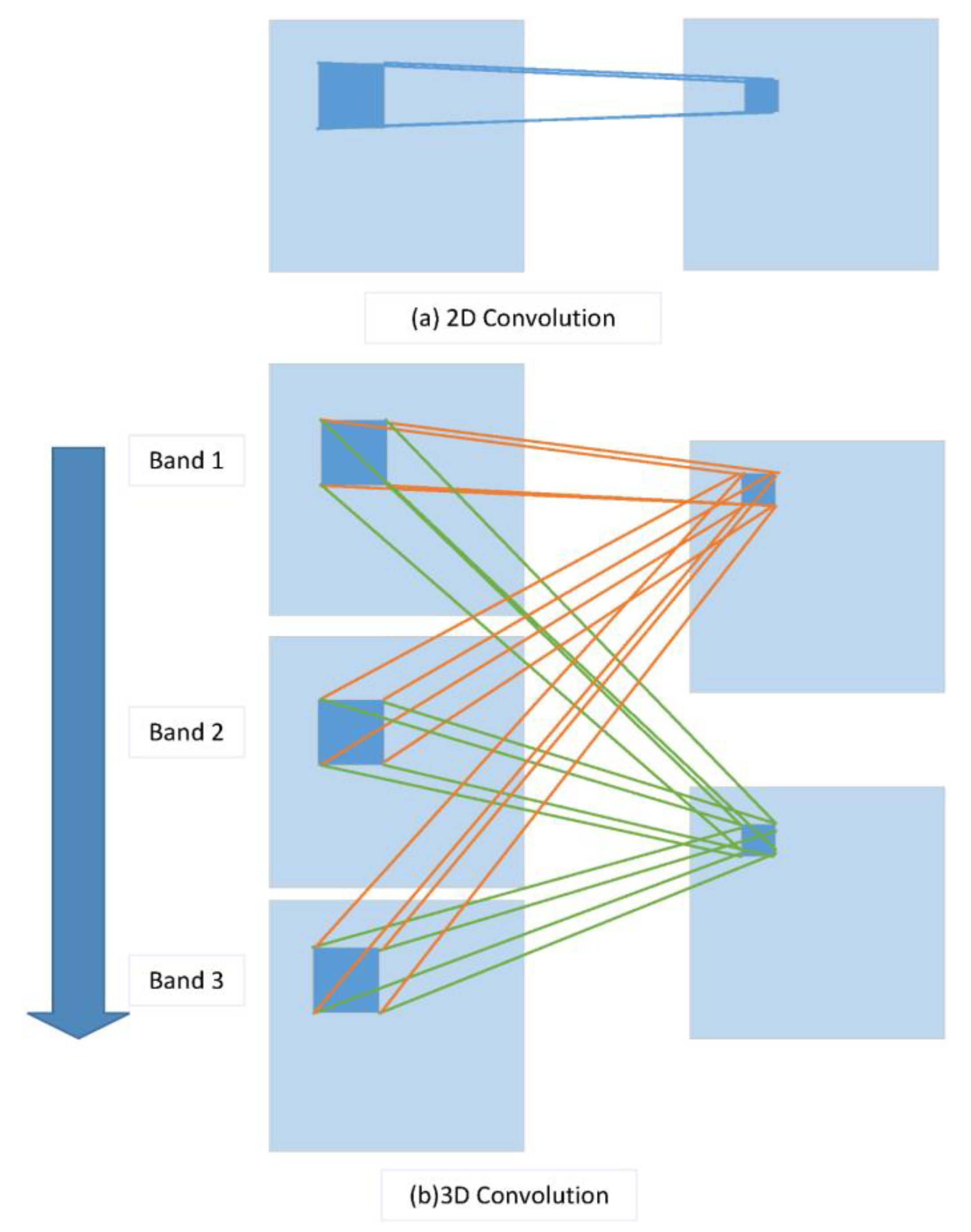
A 1D CNN extracts spectral features, whereas a 2D CNN extracts local spatial features of pixels. However, HSIs contain both abundant spatial and spectral information. For HSI classification, this means to the use of a 3D CNN, which can extract both types of information. As shown in Figure 1a, the 2D convolution sends a channel of the input image to another feature map after a convolution kernel operation. For an input image with three channels of spectral information (Band1, Band2, and Band3), a 3D convolution processes the data from three channels using two convolution kernels to obtain two characteristic maps, as shown in Figure 1b. Within the neural network, the value at position on the feature cube in the layer can be formulated as follows [12]:
where the feature map attached to the current feature map in the layer is denoted , the length and width of the convolution kernel in space are denoted by and , respectively, the size of the 3D convolution kernel along the spectral dimension is denoted , the th value of the kernel connected to the th feature cube in the preceding layer is denoted , the bias on the feature cube in the layer is denoted , and the activation function is denoted .
When a 3D CNN is applied to HSI classification, the target pixel is at the center of an -size block taken from the original pixels of the HSI as the input of the network, where is the size of the image block in the spatial domain and is the spectral dimension of the HSI. After the convolution and pooling step, the results are converted into 1D feature vectors. Finally, the feature vectors are input into a classifier to obtain the classification results.
The above operations describe the general process of a 3D CNN-based deep learning method. The key to these operations is the size of the convolution kernel, because features determine accuracy. Taking [12] as an example, a convolution kernel of or similar size is used to learn the spectral and spatial features at the same time. Distinguished from obtaining the spectral and spatial features together, the proposed framework uses the CNN to learn the spectral and spatial features separately to extract more discriminative features. Next, we explain how to use different-sized kernels to achieve this.
A kernel of size learns the spectral features from a HSI. Local spatial features exist in the HSI space, and the 2D convolution process aims to extract the local spatial features. However, the convolution with a kernel size of does not extract any spatial features because it does not consider the relationship between pixels and their neighbors in the spatial field. Nevertheless, the convolution of a kernel size of can make linear combinations or integrate spatial information for each pixel in a spatial field. Therefore, for 3D hyperspectral data a kernel of size of extracts spectral features and perfectly retains the spatial features.
The spectral information is encoded within bands of hyperspectral data, which is the reason for the high dimensionality of hyperspectral data. However, after spectral features are learned by a kernel of size , the high dimensions of the hyperspectral data can be reduced by a 3D CNN and a reshaping operation. The key to reducing high dimensionality lies in the method of padding the 3D convolution layer. “Same” and “valid” are two frequently used ways of padding. “Same” denotes convolution results at the reserved boundary, which usually cause the output shape to be the same as the input shape. “Valid” represents only effective convolution; that is, the boundary data are not processed. The valid convolution is used to reduce dimensions and retain extracted spectral features and raw spatial information.
A kernel of size of learns the spatial features from a HSI after the spectral features have been learned. By reducing the high dimension, a kernel of size can learn the spatial features from the reserved spatial information of the previous step.
In short, our framework uses a 3D convolution layer of a kernel of size to learn the spectral features. Next, the high dimension of the feature maps is reduced, and then a 3D convolution layer of a kernel of size learns the spatial features. Finally, the classification result is obtained by average pooling, flattening, and a fully-connected layer.
2.2. Going Deeper with Densely-Connected Structures
2.2.1. Densely-Connected Structure
Assume that the CNN has convolution layers, is the output of the layer and represents the complex nonlinear transformation operations in the convolution layer. The connected structure of the traditional CNN is such that the output of the layer is the input of the layer:
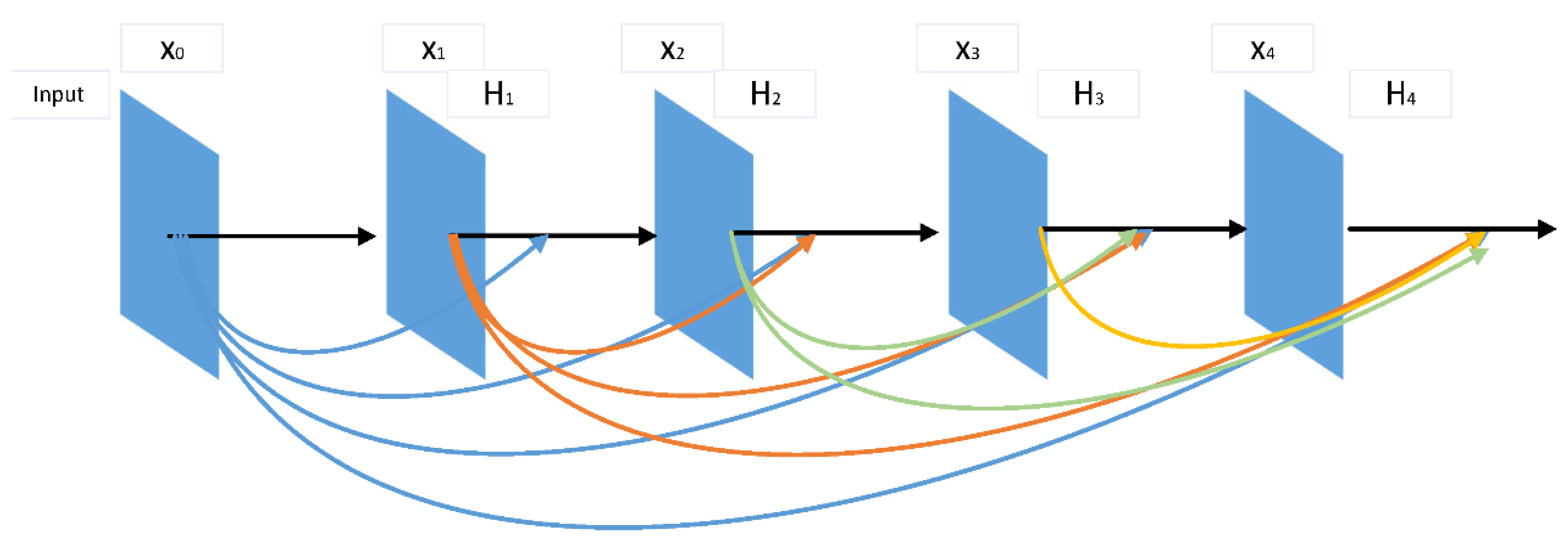
As shown in Figure 2, DenseNet [17] uses an extremely densely-connected structure, with the feature map of the output of the zeroth to the layers acting as the input to the layer. The connected structure is formulated as
DenseNet combines the number of channels and leaves the value of the feature maps unchanged. To promote the down-sampling of the framework, DenseNet is divided into multiple densely-connected blocks called Dense Blocks, with a transition layer connecting each one. Each layer of DenseNet directly connects to the input and the prior layer, resulting in a hidden deep supervision. This connected structure reduces the phenomenon of gradient disappearance and thus constructs a deeper network. In addition, DenseNet has a regularizing effect that inhibits overfitting.
2.2.2. Separately Learning Deeper Spectral and Spatial Features
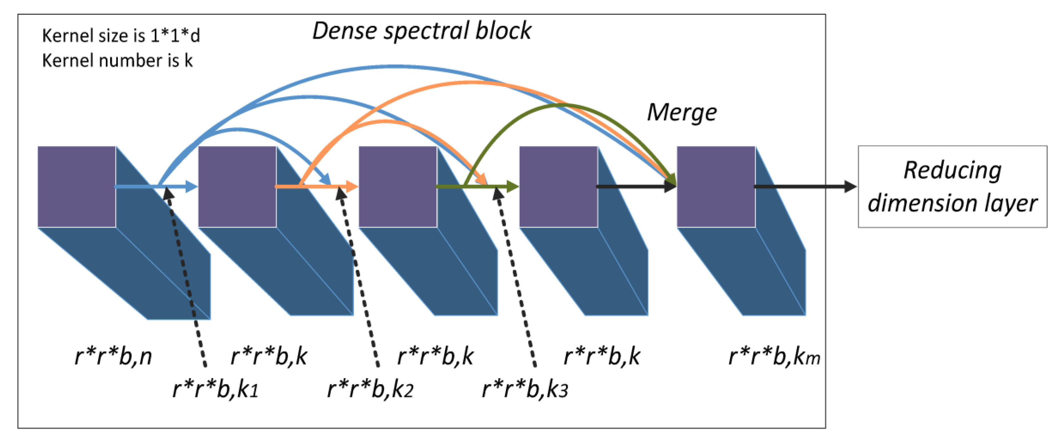
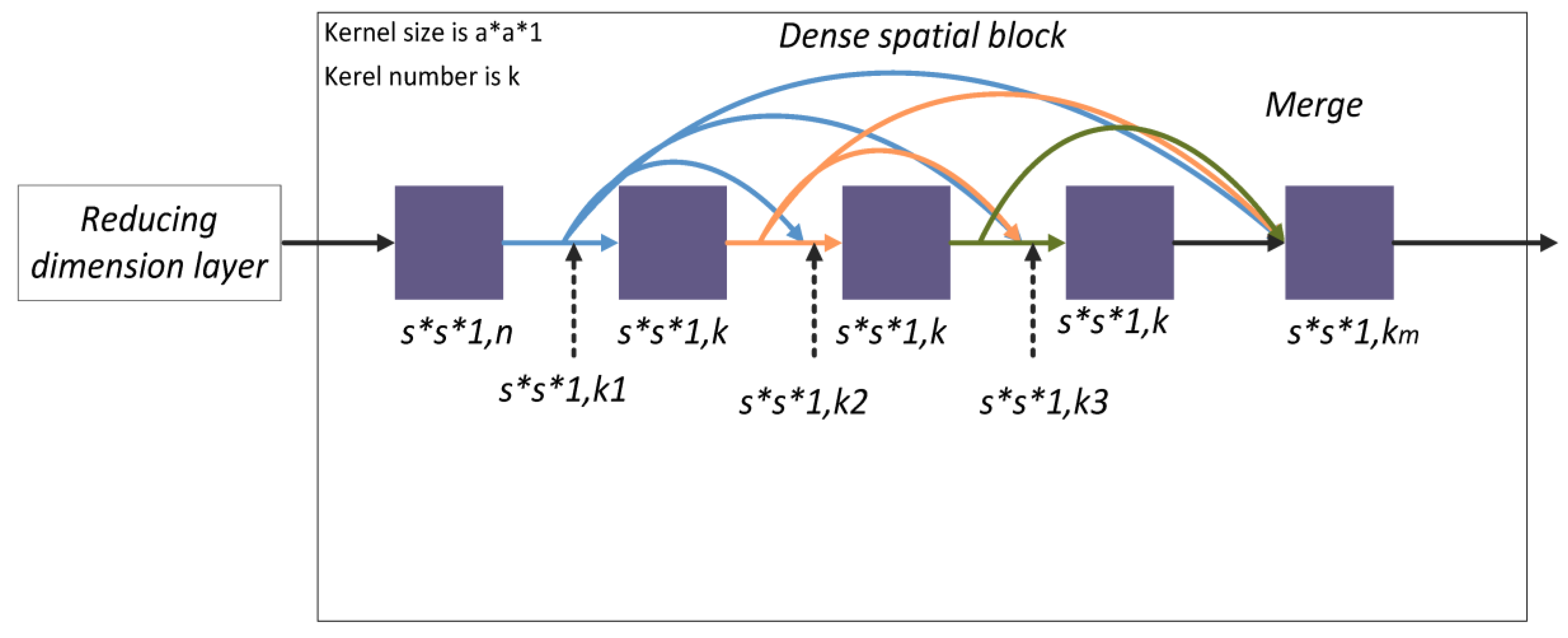
The densely-connected structure is used to learn deeper spectral and spatial features from HSIs. The small cube block is the input of our model. To improve down-sampling and separately learn the deeper spatial and spectral features of HSIs, we divided the model into two densely-connected blocks called dense spectral and spatial blocks.
Dense spectral blocks identify the deeper spectral features between multiple channels of a HSI. The first 3D convolution layer processes the original pixel data of size to produce feature maps with size . The maps are the input to a dense spectral block denoted , where the subscript 1 represents the data in the dense spectral block of the model and the superscript 0 represents the data in the starting position of the dense spectral block. The 3D convolution layers (including the first 3D convolution layer) use kernels of size to learn deeper spectral features. The convolution layer in the dense spectral block is recorded as . Since the model is densely connected, the input of the layer is
As shown in Figure 3, the size of the input and output feature maps of each composite convolution layer is the constant value and the number of output feature maps is also a constant, k. However, the number of input feature maps increases linearly with the number of composite convolution layers. The number of the input feature maps can be formulated as follows:
where is the index of the initial feature map. Through the dense spectral block, the channel feature maps merge to become , and successfully learn deeper spectral features and keep the spatial information.
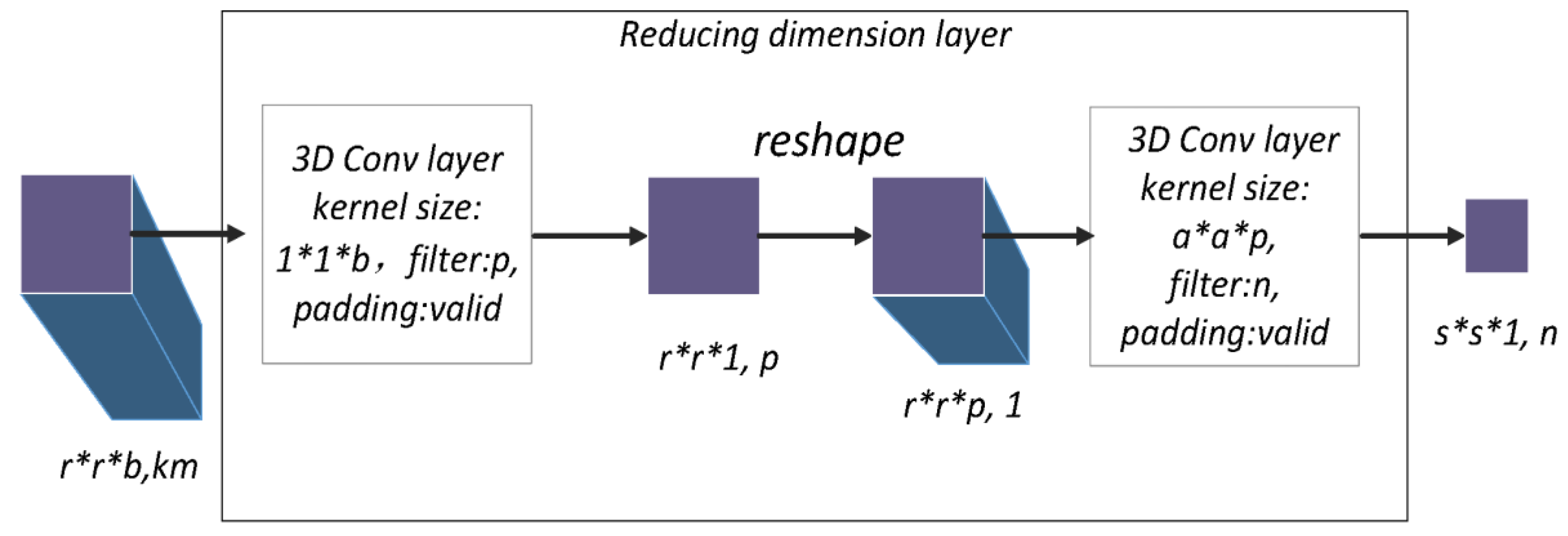
The reducing dimensional layer connects the dense spectral block and dense spatial block. The aim is to compress the model and reduce the high dimensionality of feature maps. Inside the dense spectral and spatial blocks, the method of padding a 3D convolution layer is “same”, which is the reason the output sizes are constant (). However, in reducing the dimensional layer, the method used for padding the 3D convolution layer is “valid” to change the size of feature maps.
As shown in Figure 4, feature maps with a size of proceed through the 3D convolution layer, which has a kernel size of and a kernel number . Due to the 3D convolution layer with “valid” padding, the results is p feature maps of size . Through a reshaping operation, channels of feature maps become one channel of size . Then, a 3D convolution layer that has a kernel size of and a kernel number n transforms the feature map to an with channels.
In summary, through two 3D convolution layers with “valid” padding and reshaping, the size of the feature maps becomes , which reduces the space size, the large number of channels, and the high dimensionality of the data blocks. This process facilitates the extraction of new features from the dense spatial block.
The dense spatial block learns the deeper spatial features of the HSI. For the convolution layer in the dense spatial block, the kernel size is , and the number of kernels is also . The convolution layer in the dense spatial block is termed . The output of the convolution layer of the th layer in the dense spatial block is given by
As shown in Figure 5, the size of the input and output feature maps of each convolution layer are of a constant size () and the number of output feature maps is also constant with value k. The number of input feature maps is the same as in Equation (5).
2.3. Going Faster and Preventing Overfitting
There are a large number of training parameters in our framework, which means long training times and a tendency to overfit the training sets. Here, we explain how our framework is able to be faster and prevent overfitting.
We selected PReLU as the activation function [20]. It introduces a very small number of parameters on the basis of the ReLU [21]. Its formula is
where is the input of the nonlinear activation on the th channel and is a learnable parameter that determines the slope of the negative part. PReLU adopts the momentum method when updating :
For the updating formula, is the momentum and is the learning rate. When updating , the weight decay should not be used because may tend to zero. is used as the initial value. Although ReLU is a useful nonlinear function, it hinders counter-propagation, whereas PReLU makes the model converge more quickly. Batch normalization (BN) [22] adds standardized processing to the input data of each layer in the training process of a neural network and means that the gradients converge faster, saving time and resources during model training. For the proposed framework, BN and PReLU are added before the 3D convolution layer, except for the first 3D convolution layer.
Early stopping and the dynamic learning rate are also used when training a model. Stopping early means that, after a certain number of epochs (such as 50 in this paper), if the loss is no longer decreasing, the training process will be stopped early. This reduces the training time as well as preventing overfitting. We adopted a variable learning rate because the step size should decrease as the result approaches an optimal value. With a better initial learning rate, the learning rate is halved when the precision does not increase after a certain number of epochs (such as 10 epochs in this paper). If precision no longer increases after a certain number of epochs, the learning rate will be reduced by half again and will loop until it is less than the set minimum learning rate. In this paper, the minimum learning rate was set to 0; that is, the learning rate looped until the maximum number of epochs was reached.
Since the network of the proposed model is deeper, we used a dropout layer [23] before the full connection layer to reduce the possibility of overfitting. We set the dropout rate to 50% because at this point the network structure randomly generated by the dropout layer is the greatest and produced the best results. Cross-validation prevents overfitting for complex models, so we divided our datasets into a training, validation, and test datasets for cross-validation.
2.4. Fast Dense Spectral–Spatial Convolution Framework
2.4.1. Objective Function
HSI classification presents a typical classification problem. For such problems, a cross-entropy loss function is commonly used to measure the difference between predicted value and real value to optimize the parameters of the model. In this paper, the predicted value of the FDSSC framework is a vector, , where , and is formulated as follows:
where is the parameter of the FDSSC model to be optimized and is the number of categories to be classified. Since HSI classification requires multiple classification discriminations, we performed a softmax regression, with the loss function
where denotes the size of the mini-batch, the number of categories to be classified, the th deep feature belonging to the th class, the jth column of the weights W in the last fully connected layer, and the bias term.
Therefore, the objective function of the FDSSC framework, , is
2.4.2. Fast Dense Spectral–Spatial Convolution Network for Classification of Labeled Pixels
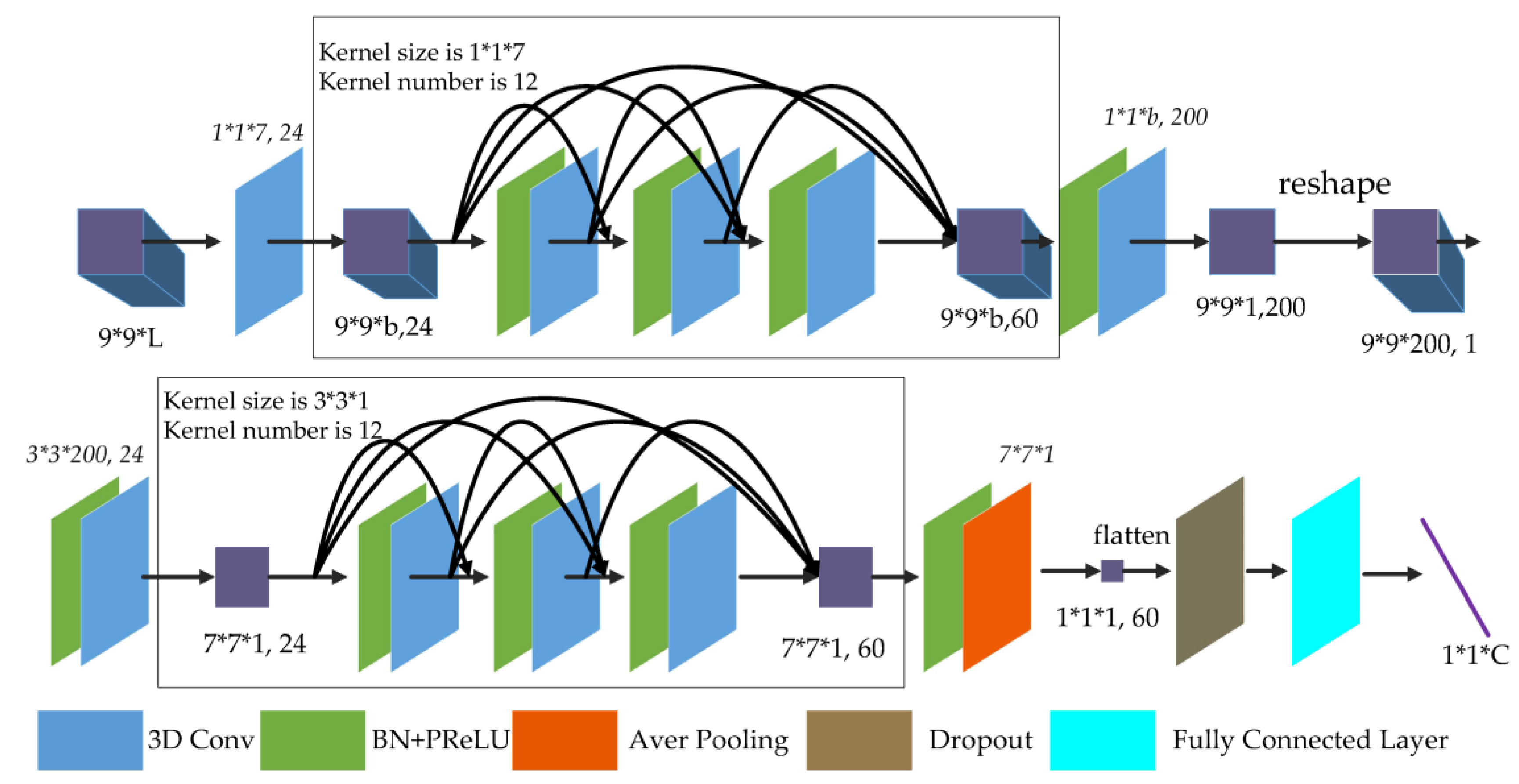
For a hyperspectral image with channels and size, r was selected as 9; that is, a target pixel served as the center of a small cube with size selected from the original pixel data as the input of the neural network. In this paper, the convolution kernel number of dense blocks was 12 and the number of convolution layers of dense blocks was 3. The FDSSC network is shown in Figure 6.
For the following detailed explanation, BN and PReLU are added before all convolution and average pooling layers, except the first 3D convolution layer. As shown in Figure 6, the original data pass through the first 3D convolution layer generated feature maps of size because the stride of the first convolution layer is and the method of padding is “valid.” For the convolution layers of the dense spectral block, the kernel size is , the kernel number is 12, the method of padding is “same”, and the stride is , so the output of each convolution layer is 12 feature maps containing the learned spectral features. Merging all output and the initial input, the size of feature maps is unchanged and the number of channels is .
In reducing the dimensional layer, 60 feature maps with a size of proceed through the 3D convolution layer, which has a kernel size of and a kernel number of 200. Since the 3D convolution layer has “valid” padding, there are 200 feature maps. Through a reshaping operation, the channels of feature maps become one feature map with a size of . Next, a 3D convolution layer with and a size of transformed the feature map into a with channels.
For the convolution layers of the dense spatial block, the kernel size is , the kernel number is 12, and the padding is “same,” so each output of the convolution layers is 12 feature maps to learn the deeper spatial features. Similar to the dense spectral block, 60 feature maps with a size of are produced.
Finally, the 3D average pooling layer with a pooling size changes the size of the feature maps to . Through the flattening operation, dropout layer, and fully-connected layers, a prediction vector is produced, where is the number of categories to be classified.
2.4.3. Fast Dense Spectral–Spatial Convolution Framework
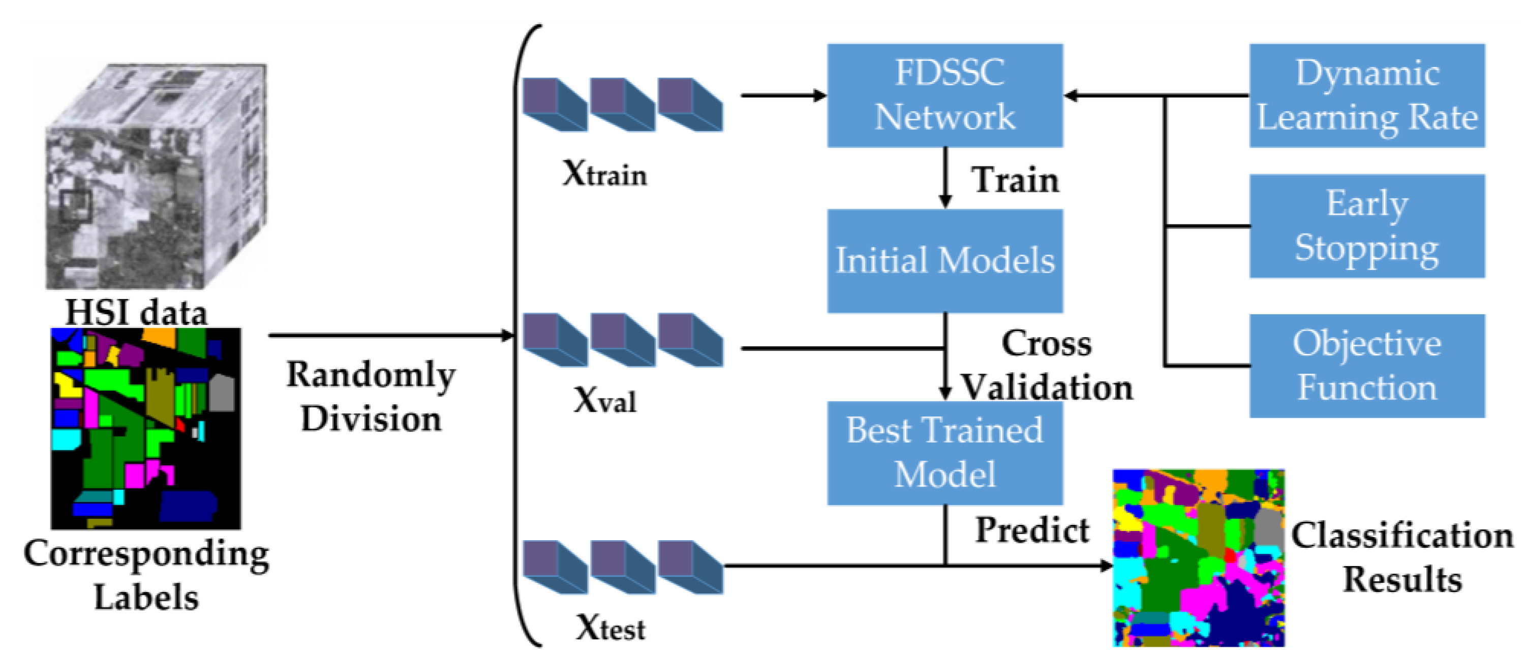
Summarizing the above steps, we have proposed a framework that learns deeper spectral and spatial features while reducing the training time compared to deep learning CNN-based methods. The FDSSC framework is shown in Figure 7.
The partition of HSI data and labels is the first step of the proposed framework. For cross-validation, we randomly divided the labeled pixels and corresponding labels into training, validation, and testing datasets selected with size from the original HSIs, denoting these datasets , , and , respectively.
Taking the cross-entropy as the objective function, and were utilized to train the FDSSC network to obtain the best FDSSC model under the control of the dynamic learning rate and early stopping. The FDSSC framework was only used to optimize the parameters of the model through back-propagation, and tested the initial trained models using . Through cross-validation, the FDSSC could obtain the best-trained model. Finally, FDSSC made use of the best-trained model to obtain three evaluation indices of performance by and classified all datasets.
Combining Figure 6 and Figure 7 clarifies the technical advantages of the proposed method. First, the FDSSC network only uses a convolution layer and an average pooling layer to learn features and the fully-connected layer as a classifier, so it is an end-to-end framework and reduces high dimensions without complicated feature engineering. Second, because of the densely-connected method, the FDSSC network has a deeper structure resulting in extremely efficient performance. Finally, the convergence rate of the model is very fast because of the BN and PReLU applied to the FDSSC network and dynamic learning rate, and early stopping. Therefore, the training time of the proposed framework is shorter, and although the FDSSC model has a high quantity of parameters, it lacks overfitting on account of the dropout layer in the FDSSC network, early stopping, and cross-validation.
3. Datasets and Experimental Setup
3.1. Datasets
In our experiments, we used the Indiana Pines (IN), the University of Pavia (UP, Pavia, Italy), and the Kennedy Space Center (KSC, Merritt Island, FL, USA) datasets (Supplementary Materials). The KSC data were obtained by the AVIRIS spectrometer in Florida in 1996. The size of the original data is and it contains 13 kinds of ground cover. Table 1 summarizes the categories and image counts for each. The University of Pavia data are from flights of the ROSIS sensor over Pavia in Northern Italy in 2003. The original data has size with spatial resolution 1.3 m. Table 2 shows the nine types of ground cover and the image counts for each. The IN data were obtained by the AVIRIS spectrometer in Northwestern Indiana in 1996. The original data size is , with 16 kinds of ground cover. Table 3 provides detailed category information.
3.2. Experimental Setup for Classification of Labeled Pixels
We configured our FDSSC framework for the classification of labeled pixels as follows: The kernel number of the dense blocks was set to k = 12 and the number of convolution layers in each dense block was set to 3. From the possible batch sizes of (16, 20, 24, 32, 64), 32 was selected in view of the performance of our graphics processing unit (GPU) and test accuracy. The time limit of the initial training epochs was 400, but on the basis of our prior experimental results the best precision was reached within 80 epochs, so the number of epochs used during training was only 80.
Taking the IN data as an example, the RMSprop [24], Adam [25], and Nadam [26] optimizers yielded final precision results of 99.777%, 99.665%, and 99.567%, respectively. Thus, we chose the RMSprop optimizer. The initial learning rate was 0.0003. We used the He normal distribution initialization method [20] as the initialization method for all convolution layers in the neural network model. We used the Xavier normal distribution initialization method [27], also known as the Glorot normal distribution initialization method, for the fully-connected layer.
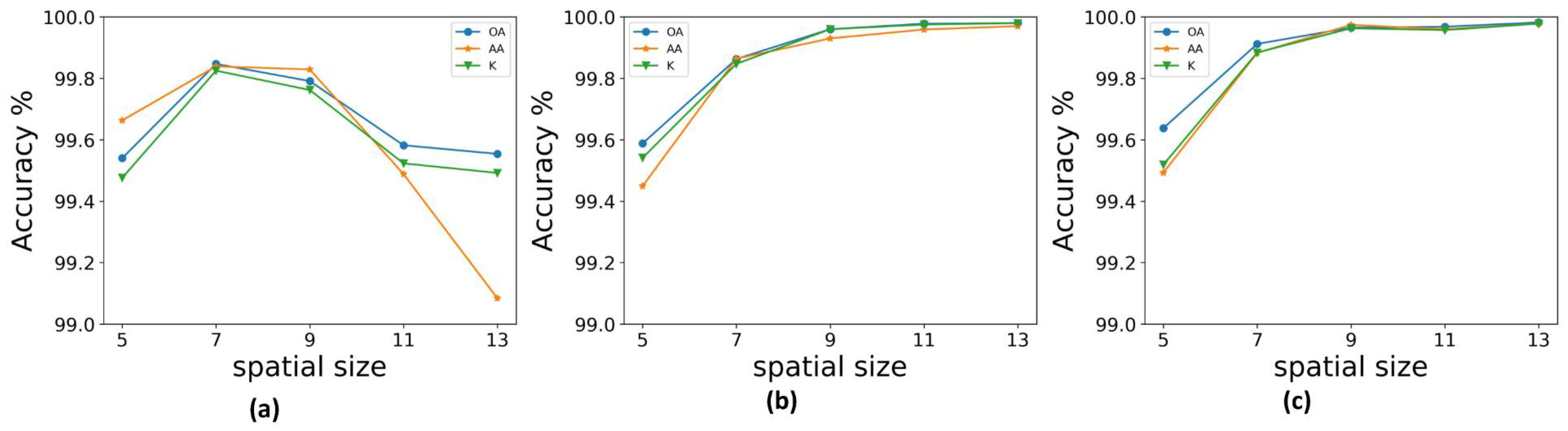
For the 3D CNN used for HSI classification, the spatial size of the input sample is an important factor affecting the HSI classification. Using the three datasets, we set r to 5, 7, 9, 11, and 13; that is, spatial sizes of , , , , and for the input sample. We measured the overall accuracy (OA), the average accuracy (AA), and kappa coefficient (K) for each dataset. Figure 8a shows that with an increase in the size of the input space the classification accuracy on the IP dataset began to fall after . For the KSC dataset, Figure 8b shows that the classification accuracy increased with increasing size of the input space, but after , the accuracy reached 99.9% and then increased by less than 0.01%. The UP dataset showed very little increase in accuracy after , as shown in Figure 8c. Therefore, we chose as the size for testing the performance of the FDSSC framework.
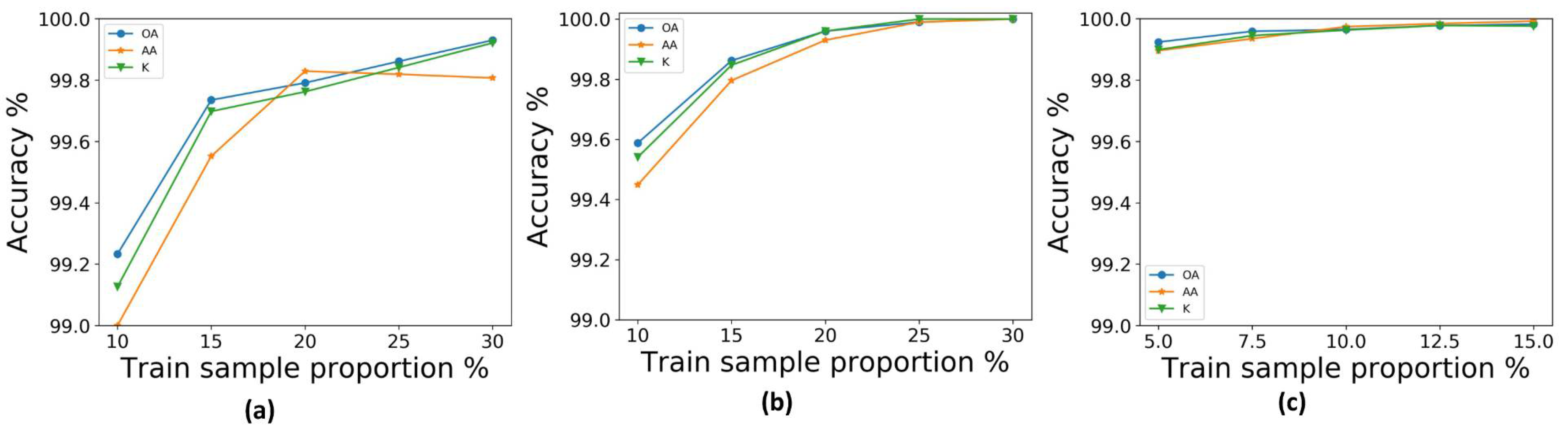
Deep learning algorithms rely greatly on the training samples. The more data used in training, the higher the test accuracy. We tried different training sample sizes on the three datasets, using 10%, 15%, 20%, 25%, and 30% on the IP and KSC datasets. For the UP dataset, the large number of data samples meant that the accuracy of the three training samples reached 99.97% with a training sample size of only 15%. Thus, we chose to test with sample sizes of 5%, 7.5%, 10%, 12.5%, and 15%. Figure 9a shows that, as the training sample size increased on the IN dataset, the OA and AA also increased, but the kappa coefficient decreased after 20%. As shown in Figure 9b, after the 20% training sample size with the KSC dataset, the OA, AA, and kappa coefficient reached 99.9%, and when the training sample size increased to 30%, all three reached 100%. As shown in Figure 9c, for the UP dataset, the OA, AA, and kappa coefficent reached 99.9% at a 10% training sample size. At a 15% training sample size, all three datasets achieved 0.01–0.02% higher accuracy than at 10%. Therefore, for the FDSSC framework, although larger training sample sizes improve accuracy to a degree, accuracy was over 99.9% for the KSC dataset with only a 20% training sample size, with the same accuracy for the UP dataset at only 10%. Even substantial increases in training time brought only very limited increases in accuracy. Therefore, we chose a training sample size of 20% for the IN and KSC datasets and 10% for the UP dataset; for all of the HSI datasets the validation dataset size was half the training dataset size and the remainder comprised the test dataset.
4. Experimental Results and Discussion
In our experiment, we compared the proposed FDSSC framework to other deep-learning-based methods, that is, SAE-LR [8], CNN [9], 3D-CNN-LR [11], and the state-of-art SSRN method [13] (only for labeled pixels). SAE-LR was implemented with Theano [28]. CNN, SSRN, and the proposed FDSSC were implemented with Keras [29] using TensorFlow [30] as a backend. 3D-CNN-LR was obtained from the literature [11]. In the following, the detailed classification accuracy and training times are shown and discussed.
4.1. Experimental Results
In our experiment, we randomly selected 10 groups of training samples from the KSC, UP, and IN datasets. Experimental results are given in the form “mean ± variance.” The training and testing time results were obtained using the same computer, which was configured with 32 GB of memory and a NVIDIA GeForce GTX 1080Ti GPU. The OA, AA, and kappa coefficient were used to determine the accuracy of the classification results. Work from [9] was denoted CNN. The input spatial size is important for the 3D convolution method. Therefore, to ensure a fair comparison, an appropriate spatial size was chosen for each method. For the SSRN method, the classification accuracy increases with the spatial size, so we used an input spatial size of , which was the same as that of the FDSSC framework. Figure 10, Figure 11 and Figure 12 show classification maps for each of the methods.
The comparison of deep-learning-based methods relies heavily on training data. Sometimes a method may appear better, but in reality it simply has more training data. Therefore, the same amount of training data should be used for all of the methods compared. However, for some methods, such as the CNN for the IN dataset, when we used the same proportion to train the model the overall accuracy would fall by approximately 2%. Therefore, in order to obtain the best accuracy for each model, in these cases we use the same training proportion as previously used in the literature. For SAE-LR, the split ratio of training, validation, and testing data was 6:2:2; for a CNN, the split ratio was 8:1:1; for the SSRN method, the split ratio was 2:1:7 for the IN and KSC datasets, and 1:1:8 for the UP dataset; for the proposed FDSSC framework, we used 20% of the labeled pixels as the training set, and 10% and 70% for validation and testing datasets, respectively, for the IN and KSC datasets, and 10%, 5%, and 85% for the UP dataset. Table 4 shows the OA, AA, and kappa coefficient for the different methods for the KSC, IN, and UP datasets. From Table 4, it can be clearly seen that the proposed FDSSC framework is superior to SAE-LR, CNN, and 3D-CNN-LR methods. For the state-of-the-art SSRN method, we note slight improvements of 0.02%, 0.37%, and 0.04% for the KSC, IN, and UP datasets, respectively. There is no more obvious improvement because the OAs of two of the methods are higher than 99%.
Table 5 summarizes the average training times, training epochs, and testing times of 10 runs of the SAE-LR, CNN, SSRN, and FDSSC methods. SAE-LR was trained with 3300 epochs of pre-training and 400,000 epochs of fine-tuning [8]; the training time for fine-tuning was only 61.7 min. For a CNN [9], the training process of this model converged in almost 40 epochs, but in our experiments the model trained with 120 epochs achieved the best accuracy. The SSRN method needed 200 training epochs [13] and the FDSSC framework only needed 80 training epochs to achieve the best accuracy. Therefore, the FDSSC training time was less than that of other deep-learning-based methods. The hyperspectral data became larger from KSC to UP, and the time difference of the FDSSC framework increased compared with other deep-learning-based methods. Therefore, the larger the hyperspectral data, the more time was reduced by the FDSSC framework.
4.2. Discussion
In terms of accuracy of the HSI classification methods, for deep-learning-based methods, our experiments show that the deeper the framework is, the higher the classification accuracy. The proposed FDSSC framework is obviously superior to the SAE-LR, CNN, and 3D-CNN-LR methods. Compared with the SSRN method, which has state-of-the-art accuracy, the FDSSC method improves OA and AA by 0.40% and 11.23%, respectively, for the IN dataset. It is precisely because of the greater depth of the FDSSC network that the spectral and spatial features of HSIs are more effectively utilized, with better feature transfer between the convolution layers. Although the training size of the SAE-LR and CNN methods are greater than that of the FDSSC framework, the FDSSC framework has higher accuracy than the SAE-LR and CNN methods. In addition, compared with the 24 kernel numbers of the SSRN method, the FDSSC framework uses only 12 kernel numbers, and the model is narrower.
In terms of the training time, the FDSSC framework takes less time and has the characteristics of fast convergence. Many deep learning methods, such as the SSRN, use ReLU, but the FDSSC framework uses PReLU. Problems with ReLU include neuronal death and the offset phenomenon. The former occurs because when , ReLU will be in the hard-saturation area. As training advances, part of the input will fall into the hard-saturation area, meaning that the corresponding weight cannot be updated. The latter occurs because the mean of the activations is always greater than zero. Neuronal death and offset phenomena jointly influence the convergence of a network. Compared with ReLU, PReLU converges faster because the output of PReLU is closer to zero. BN and dynamic learning rate are the other reasons for fast convergence. Thus, compared with the 400,000 epochs required by the SAE-LR method, 200 epochs required by the SSRN method, and 120 epochs by the CNN, the FDSSC framework needs only 80 epochs to obtain the best accuracy, which leads to a shorter training time than other deep-learning-based methods.
Therefore, taking both accuracy and running time into account, we conclude that the FDSSC framework has state-of-the-art accuracy with less required training time than methods achieving similar accuracy.
5. Conclusions and Future Work
In this paper, we propose an end-to-end, fast, and dense spectral–spatial convolution framework for HSI classification. The most significant features of the proposed FDSSC framework are depth and speed. Furthermore, the FDSSC framework has no complicated mechanism for reducing the dimensionality, and instead uses original 3D pixel data directly as input. The proposed framework uses two different dense blocks to extract abundant spatial features and spectral features in HSIs automatically. The densely-connected arrangement of dense blocks deepens the network, reducing the problem of gradient disappearance. The result is that the classification precision of the FDSSC framework reaches a very high level. We introduced BN, dropout layers, and dynamic learning rates, and adopted PReLU as the activation function of the neural network to initialize fully-connected layers. These improvements led the FDSSC framework to converge faster and prevented overfitting, such that only 80 epochs were needed to achieve the best classification accuracy.
The future direction of our work is hyperspectral data segmentation, aimed at segmenting hyperspectral data based on our classification work. We plan to study an end-to-end, pixel-to-pixel deep-learning-based method for hyperspectral data segmentation.
Supplementary Materials
The Kennedy Space Center, Indiana Pines, and University of Pavia datasets are available online at http://www.ehu.eus/ccwintco/index.php?title=Hyperspectral_Remote_Sensing_Scenes. They are also available online at https://0-www-mdpi-com.brum.beds.ac.uk/2072-4292/10/7/1068/s1.
Author Contributions
All the authors made significant contributions to this work. W.W. and S.D. conceived and designed the experiments; S.D. performed the experiments; W.W. and Z.J. analyzed the data; and L.S. contributed analysis tools.
Funding
This study was funded by the Laboratory of Green Platemaking and Standardization for Flexography Printing (grant no. ZBKT201710).
Acknowledgments
The authors are grateful to the editor and reviewers for their constructive comments, which have significantly improved this work.
Conflicts of Interest
The authors declare no conflicts of interest. The founding sponsors had no role in the design of the study; in the collection, analyses, or interpretation of data; in the writing of the manuscript; nor in the decision to publish the results.
References
- Plaza, A.; Du, Q.; Chang, Y.; King, R.L. High Performance Computing for Hyperspectral Remote Sensing. IEEE J. Sel. Top. Appl. Earth Observ. Remote Sens. 2011, 4, 528–544. [Google Scholar] [CrossRef]
- Nolin, A.W.; Dozier, J. A Hyperspectral Method for Remotely Sensing the Grain Size of Snow. Remote Sens. Environ. 2000, 74, 207–216. [Google Scholar] [CrossRef]
- Mohanty, P.C.; Panditrao, S.; Mahendra, R.S.; Kumar, S.; Kumar, T.S. Identification of Coral Reef Feature Using Hyperspectral Remote Sensing. In Proceedings of the SPIE-The International Society for Optical Engineering, New Delhi, India, 4–7 April 2016; pp. 1–10. [Google Scholar]
- Melgani, F.; Bruzzone, L. Classification of Hyperspectral Remote Sensing Images with Support Vector Machines. IEEE Trans. Geosci. Remote Sens. 2004, 42, 1778–1790. [Google Scholar] [CrossRef]
- Li, W.; Chen, C.; Su, H.; Du, Q. Local Binary Patterns and Extreme Learning Machine for Hyperspectral Imagery Classification. IEEE Trans. Geosci. Remote Sens. 2015, 53, 3681–3693. [Google Scholar] [CrossRef]
- Deng, S.; Xu, Y.; He, Y.; Yin, J.; Wu, Z. A Hyperspectral Image Classification Framework and Its Application. Inf. Sci. 2015, 299, 379–393. [Google Scholar] [CrossRef]
- Zhang, L.; Zhang, L.; Du, B. Deep Learning for Remote Sensing Data: A Technical Tutorial on the State of the Art. IEEE Geosci. Remote Sens. Mag. 2016, 4, 22–40. [Google Scholar] [CrossRef]
- Chen, Y.; Lin, Z.; Zhao, X.; Wang, G.; Gu, Y. Deep Learning-Based Classification of Hyperspectral Data. IEEE J. Sel. Top. Appl. Earth Obs. Remote Sens. 2014, 7, 2094–2107. [Google Scholar] [CrossRef]
- Makantasis, K.; Karantzalos, K.; Doulamis, A.; Doulamis, N. Deep Supervised Learning for Hyperspectral Data Classification through Convolutional Neural Networks. In Proceedings of the 2015 IEEE International Geoscience and Remote Sensing Symposium, Milan, Italy, 26–31 July 2015; pp. 4959–4962. [Google Scholar]
- Zhao, W.; Du, S. Spectral-Spatial Feature Extraction for Hyperspectral Image Classification: A Dimension Reduction and Deep Learning Approach. IEEE Trans. Geosci. Remote Sens. 2016, 54, 4544–4554. [Google Scholar] [CrossRef]
- Chen, Y.; Jiang, H.; Li, C.; Jia, X.; Ghamisi, P. Deep Feature Extraction and Classification of Hyperspectral Images Based on Convolutional Neural Networks. IEEE Trans. Geosci. Remote Sens. 2016, 54, 6232–6251. [Google Scholar] [CrossRef]
- Li, Y.; Zhang, H.; Shen, Q. Spectral-Spatial Classification of Hyperspectral Imagery with 3D Convolutional Neural Network. Remote Sens. 2017, 9, 67. [Google Scholar] [CrossRef]
- Zhong, Z.; Li, J.; Luo, Z.; Chapman, M. Spectral-Spatial Residual Network for Hyperspectral Image Classification: A 3-D Deep Learning Framework. IEEE Trans. Geosci. Remote Sens. 2017, 99, 1–12. [Google Scholar] [CrossRef]
- Zhou, X.; Li, S.; Tang, F.; Qin, K.; Hu, S.; Liu, S. Deep Learning with Grouped Features for Spatial Spectral Classification of Hyperspectral Images. IEEE Geosci. Remote Sens. Lett. 2017, 14, 97–101. [Google Scholar] [CrossRef]
- Ma, X.; Wang, H.; Wang, J. Semisupervised Classification for Hyperspectral Image Based on Multi-Decision Labeling and Deep Feature Learning. ISPRS J. Photogramm. Remote Sens. 2016, 120, 99–107. [Google Scholar] [CrossRef]
- Maltezos, E.; Doulamis, N.; Doulamis, A.; Ioannidis, C. Deep Convolutional Neural Networks for Building Extraction from Orthoimages and Dense Image Matching Point Clouds. J. Appl. Remote Sens. 2017, 11, 1–22. [Google Scholar] [CrossRef]
- Huang, G.; Liu, Z.; Weinberger, K.Q. Densely Connected Convolutional Networks. In Proceedings of the 2017 IEEE Conference on Pattern Recognition and Computer Vision (CVPR), College Park, MD, USA, 25–26 July 2017; pp. 1–9. [Google Scholar]
- Szegedy, C.; Liu, W.; Jia, Y.; Sermanet, P.; Reed, S.; Anguelov, D.; Erhan, D.; Vanhoucke, V.; Rabinovich, A. Going Deeper with Convolutions. In Proceedings of the IEEE Conference on Computer Vision and Pattern Recognition, CVPR 2015, Boston, MA, USA, 7–12 June 2015; pp. 1–9. [Google Scholar]
- He, K.; Zhang, X.; Ren, S.; Sun, J. Deep Residual Learning for Image Recognition. In Proceedings of the 2016 IEEE Conference on Computer Vision and Pattern Recognition (CVPR), Las Vegas, NV, USA, 27–30 June 2016; pp. 770–778. [Google Scholar]
- He, K.; Zhang, X.; Ren, S.; Sun, J. Delving Deep into Rectifiers: Surpassing Human-Level Performance on Imagenet Classification. In Proceedings of the 15th IEEE International Conference on Computer Vision, ICCV 2015, Santiago, Chile, 11–18 December 2015; pp. 1026–1034. [Google Scholar]
- Krizhevsky, A.; Sutskever, I.; Hinton, G.E. Imagenet Classification with Deep Convolutional Neural Networks. In Proceedings of the 26th Annual Conference on Neural Information Processing Systems 2012, Lake Tahoe, NV, USA, 3–6 December 2012; pp. 1097–1105. [Google Scholar]
- Ioffe, S.; Szegedy, C. Batch Normalization: Accelerating Deep Network Training by Reducing Internal Covariate Shift. In Proceedings of the 32nd International Conference on Machine Learning, ICML 2015, Lile, France, 6–11 July 2015; pp. 1–9. [Google Scholar]
- Srivastava, N.; Hinton, G.; Krizhevsky, A.; Sutskever, I.; Salakhutdinov, R. Dropout: A Simple Way to Prevent Neural Networks from Overfitting. J. Mach. Learn. Res. 2014, 15, 1929–1958. [Google Scholar]
- Tijmen, T.; Hinton, G. Lecture 6.5-Rmsprop: Divide the Gradient by a Running Average of Its Recent Magnitude. COURSERA Neural Netw. Mach. Learn. 2012, 4, 26–31. [Google Scholar]
- Kingma, D.P.; Ba, J.L. Adam: A Method for Stochastic Optimization. In Proceedings of the International Conference on Learning Representations 2015, San Diego, CA, USA, 7–9 May 2015; pp. 1–15. [Google Scholar]
- Sutskever, I.; Martens, J.; Dahl, G.; Hinton, G. On the Importance of Initialization and Momentum in Deep Learning. In Proceedings of the 30th International Conference on Machine Learning, ICML 2013, Atlanta, GA, USA, 16–21 June 2013; pp. 1139–1147. [Google Scholar]
- Glorot, X.; Bengio, Y. Understanding the Difficulty of Training Deep Feedforward Neural Networks. In Proceedings of the 13th International Conference on Artificial Intelligence and Statistics, AISTATS 2010, Sardinia, Italy, 13–15 May 2010; pp. 249–256. [Google Scholar]
- Al-Rfou, R.; Alain, G.; Almahairi, A.; Angermueller, C.; Bahdanau, D.; Ballas, N.; Bastien, F.; Bayer, J.; Belikov, A.; Belopolsky, A.; et al. Theano: A Python Framework for Fast Computation of Mathematical Expressions. arXiv 2016, arXiv:1605.02688. [Google Scholar]
- François, C.; Keras-Team. GitHub Repository. 2015. Available online: https://github.com/fchollet/keras (accessed on 1 June 2018).
- Abadi, M.; Agarwal, A.; Barham, P.; Brevdo, E.; Chen, Z.; Citro, C.; Corrado, G.S.; Davis, A.; Dean, J.; Devin, M.; et al. Tensorflow: Large-Scale Machine Learning on Heterogeneous Distributed Systems. arXiv, 2016; arXiv:1603.04467. [Google Scholar]
Figure 1.
(a) 2D convolution and (b) 3D convolution operations per Equation (1).

Figure 2.
Example of a DenseNet with four composite layers (l = 4).

Figure 3.
Structure of dense spectral block with three convolution layers (l = 3).

Figure 4.
Structure of reducing dimensional layer. “Filter” is the number of convolution kernels and “padding” is the strategy of supplementing zero.
Figure 4.
Structure of reducing dimensional layer. “Filter” is the number of convolution kernels and “padding” is the strategy of supplementing zero.

Figure 5.
Structure of dense spatial block with three convolution layers (l = 3).

Figure 6.
The fast dense spectral–spatial convolution (FDSSC) network for hyperspectral image (HSI) classification of labeled pixels with a input. L is the number of bands of HSI. C is the number of categories to be classified.
Figure 6.
The fast dense spectral–spatial convolution (FDSSC) network for hyperspectral image (HSI) classification of labeled pixels with a input. L is the number of bands of HSI. C is the number of categories to be classified.

Figure 7.
FDSSC Framework for HSI classification of labeled pixels. The details of the FDSSC network are shown in Figure 6.
Figure 7.
FDSSC Framework for HSI classification of labeled pixels. The details of the FDSSC network are shown in Figure 6.

Figure 8.
Accuracy with different spatial size inputs: (a) Indian Pines; (b) Kennedy Space Center; and (c) University of Pavia scenes.
Figure 8.
Accuracy with different spatial size inputs: (a) Indian Pines; (b) Kennedy Space Center; and (c) University of Pavia scenes.

Figure 9.
Accuracy with different training sample proportions: (a) Indian Pines (IN); (b) Kennedy Space Center (KSC); and (c) University of Pavia (UP) scenes.
Figure 9.
Accuracy with different training sample proportions: (a) Indian Pines (IN); (b) Kennedy Space Center (KSC); and (c) University of Pavia (UP) scenes.

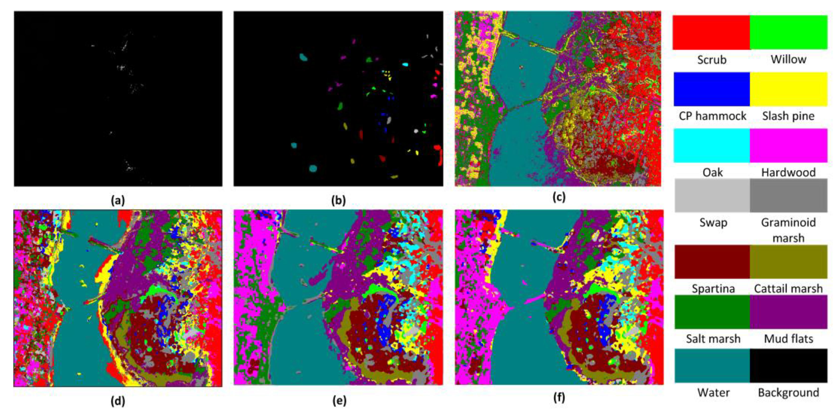
Figure 10.
Classification maps for KSC dataset: (a) real image of one band in KSC dataset; (b) ground-truth map; (c) SAE-LR, OA = 92.99%; (d) CNN, OA = 99.31%; (e) SSRN, OA = 99.94%; and (f) FDSSC, OA = 99.96%.
Figure 10.
Classification maps for KSC dataset: (a) real image of one band in KSC dataset; (b) ground-truth map; (c) SAE-LR, OA = 92.99%; (d) CNN, OA = 99.31%; (e) SSRN, OA = 99.94%; and (f) FDSSC, OA = 99.96%.

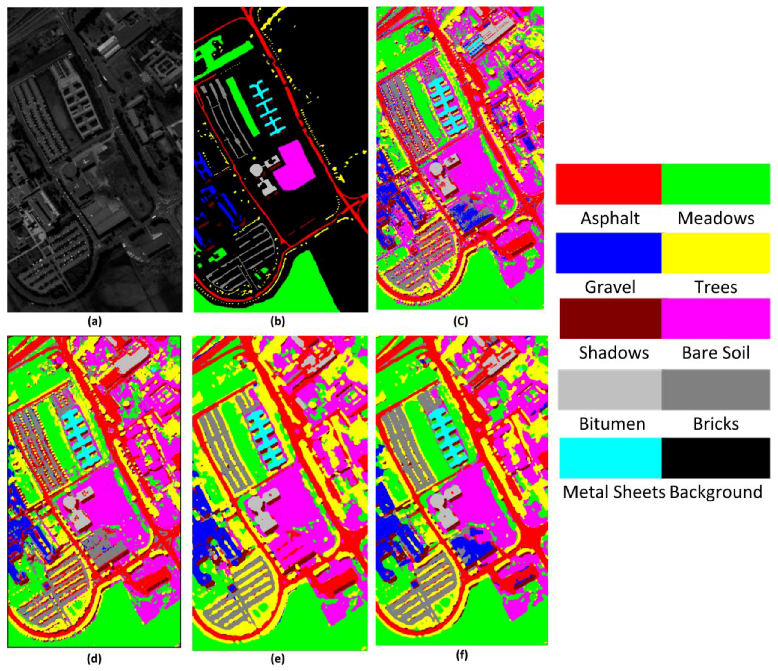
Figure 11.
Classification maps for UP dataset: (a) real image of one band in UP dataset; (b) ground-truth map; (c) SAE-LR, OA = 98.46%; (d) CNN, OA = 99.38%; (e) SSRN, OA = 99.93%; and (f) FDSSC, OA = 99.96%.
Figure 11.
Classification maps for UP dataset: (a) real image of one band in UP dataset; (b) ground-truth map; (c) SAE-LR, OA = 98.46%; (d) CNN, OA = 99.38%; (e) SSRN, OA = 99.93%; and (f) FDSSC, OA = 99.96%.

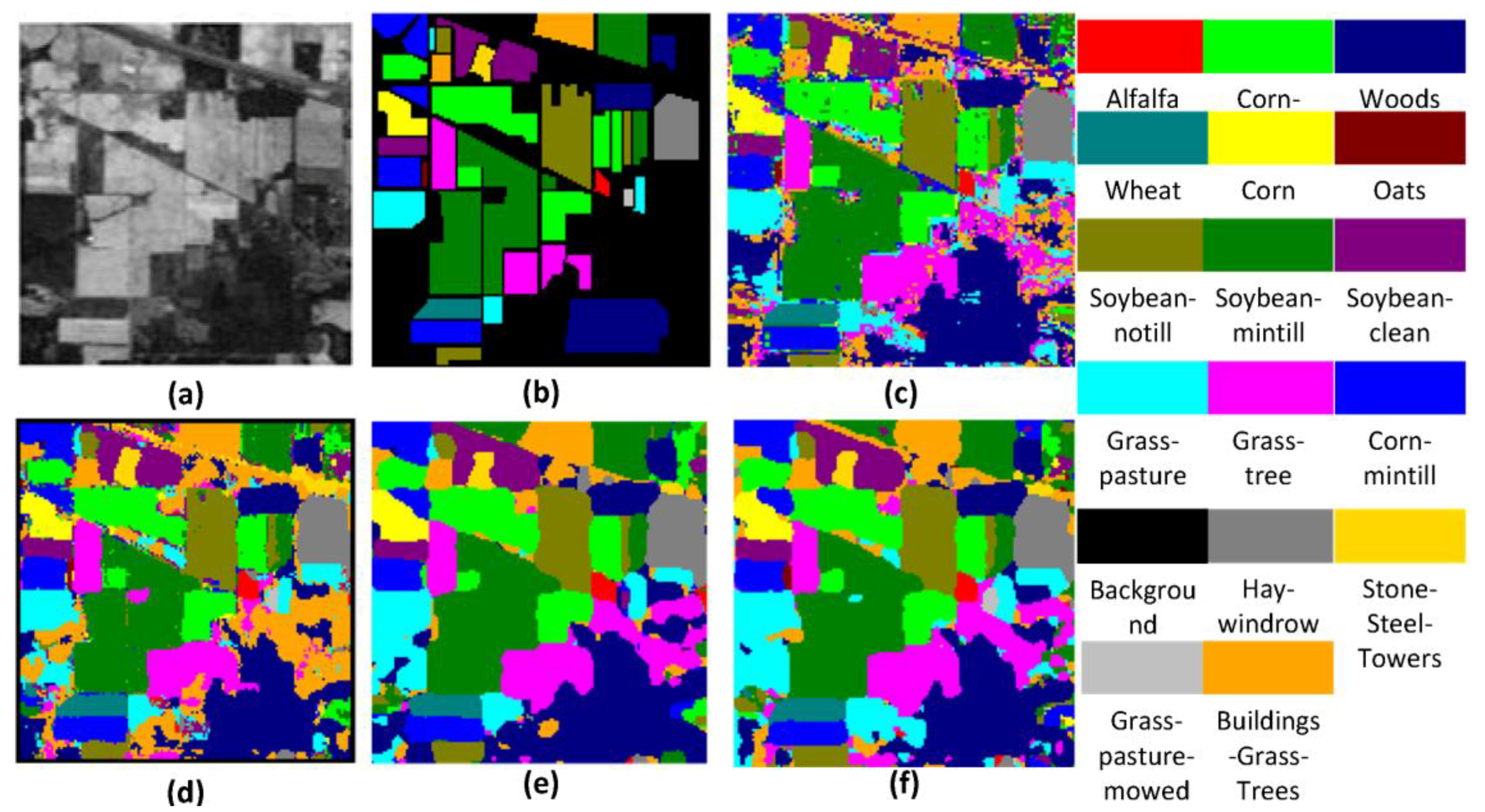
Figure 12.
Classification maps for IN dataset: (a) real image of one band in the IN dataset; (b) ground-truth map; (c) SAE-LR, OA = 93.98%; (d) CNN, OA = 95.96%; (e) SSRN, OA = 99.35%; and (f) FDSSC, OA = 99.72%.
Figure 12.
Classification maps for IN dataset: (a) real image of one band in the IN dataset; (b) ground-truth map; (c) SAE-LR, OA = 93.98%; (d) CNN, OA = 95.96%; (e) SSRN, OA = 99.35%; and (f) FDSSC, OA = 99.72%.


Table 1.
Category information for the Kennedy Space Center dataset.
| Order Number | Classification | Number of Samples |
|---|---|---|
| 1 | Scrub | 347 |
| 2 | Willow swamp | 243 |
| 3 | CP hammock | 256 |
| 4 | Slash pine | 252 |
| 5 | Oak/broadleaf | 161 |
| 6 | Hardwood | 229 |
| 7 | Swamp | 105 |
| 8 | Graminoid marsh | 390 |
| 9 | Spartina marsh | 520 |
| 10 | Cattail marsh | 404 |
| 11 | Salt marsh | 419 |
| 12 | Mud flats | 503 |
| 13 | Water | 927 |
| Total | 5211 |
Table 2.
Category information for the University of Pavia dataset.
| Order Number | Classification | Number of Samples |
|---|---|---|
| 1 | Asphalt | 6631 |
| 2 | Meadows | 18,649 |
| 3 | Gravel | 2099 |
| 4 | Trees | 3064 |
| 5 | Painted metal sheets | 1345 |
| 6 | Bare soil | 5029 |
| 7 | Bitumen | 1330 |
| 8 | Self-blocking bricks | 3682 |
| 9 | Shadows | 947 |
| Total | 42,776 |
Table 3.
Category information for the Indiana Pines dataset.
| Order Number | Classification | Number of Samples |
|---|---|---|
| 1 | Alfafa | 46 |
| 2 | Corn-notill | 1428 |
| 3 | Corn-mintill | 830 |
| 4 | Corn | 237 |
| 5 | Grass-pasture | 483 |
| 6 | Grass-trees | 730 |
| 7 | Grass-pasture | 28 |
| 8 | Hay-windrowed | 478 |
| 9 | Oats | 20 |
| 10 | Soybean-notill | 972 |
| 11 | Soybean-mintill | 2455 |
| 12 | Soybean-clean | 593 |
| 13 | Wheat | 205 |
| 14 | Woods | 1265 |
| 15 | Building-grass-trees-drives | 386 |
| 16 | Stone-steal-towers | 93 |
| Total | 10,249 |
Table 4.
Classification results of different methods for labeled pixels of the KSC, IN, and UP datasets.
Table 4.
Classification results of different methods for labeled pixels of the KSC, IN, and UP datasets.
| Method | Dataset | ||||||||
|---|---|---|---|---|---|---|---|---|---|
| KSC | IN | UP | |||||||
| OA% | AA% | K 100 | OA% | AA% | K 100 | OA% | AA% | K 100 | |
| SAE-LR [8] | 92.99 ± 0.82 | 89.76 ± 1.25 | 92.18 ± 0.91 | 96.53 ± 0.08 | 96.03 ± 0.49 | 96.05 ± 0.11 | 98.46 ± 0.02 | 97.67 ± 0.04 | 97.78 ± 0.03 |
| CNN [9] | 99.31 ± 0.04 | 98.92 ± 0.15 | 99.23 ± 0.07 | 95.96 ± 0.44 | 97.75 ± 0.05 | 95.42 ± 0.57 | 99.38 ± 0.01 | 99.23 ± 0.01 | 99.17 ± 0.02 |
| 3D-CNN-LR [11] | 96.31 ± 1.25 | 94.68 ± 1.97 | 95.90 ± 1.39 | 97.56 ± 0.43 | 99.23 ± 0.19 | 97.02 ± 0.52 | 99.54 ± 0.11 | 99.66 ± 0.11 | 99.41 ± 0.15 |
| SSRN [13] | 99.94 ± 0.07 | 99.93 ± 0.08 | 99.94 ± 0.08 | 99.35 ± 0.19 | 88.44 ± 2.35 | 99.26 ± 0.22 | 99.93 ± 0.03 | 99.91 ± 0.05 | 99.91 ± 0.04 |
| FDSSC | 99.96 ± 0.06 | 99.94 ± 0.10 | 99.95 ± 0.07 | 99.75 ± 0.13 | 99.67 ± 0.15 | 99.72 ± 0.15 | 99.97 ± 0.02 | 99.96 ± 0.03 | 99.96 ± 0.03 |
Table 5.
Training and testing time of different methods for three datasets.
| Dataset | Time | SAE-LR | SSRN | CNN | FDSSC |
|---|---|---|---|---|---|
| KSC | Training | 61.7 m | 329.3 s | 313.6 s | 201.2 s |
| Testing | 0.12 s | 1.79 s | 1.83 s | 2.57 s | |
| IN | Training | 142.2 m | 720.5 s | 441.2 s | 423.7 s |
| Testing | 0.05 s | 4.14 s | 2.19 s | 5.56 s | |
| UP | Training | 115.2 m | 1189.8 s | 1799.2 s | 498.2 s |
| Testing | 0.08 s | 12.56 s | 2.22 s | 15.51 s | |
| Training epochs | 400,000 | 200 | 120 | 80 | |
© 2018 by the authors. Licensee MDPI, Basel, Switzerland. This article is an open access article distributed under the terms and conditions of the Creative Commons Attribution (CC BY) license (http://creativecommons.org/licenses/by/4.0/).
Share and Cite
MDPI and ACS Style
Wang, W.; Dou, S.; Jiang, Z.; Sun, L. A Fast Dense Spectral–Spatial Convolution Network Framework for Hyperspectral Images Classification. Remote Sens. 2018, 10, 1068. https://0-doi-org.brum.beds.ac.uk/10.3390/rs10071068
AMA Style
Wang W, Dou S, Jiang Z, Sun L. A Fast Dense Spectral–Spatial Convolution Network Framework for Hyperspectral Images Classification. Remote Sensing. 2018; 10(7):1068. https://0-doi-org.brum.beds.ac.uk/10.3390/rs10071068
Chicago/Turabian StyleWang, Wenju, Shuguang Dou, Zhongmin Jiang, and Liujie Sun. 2018. "A Fast Dense Spectral–Spatial Convolution Network Framework for Hyperspectral Images Classification" Remote Sensing 10, no. 7: 1068. https://0-doi-org.brum.beds.ac.uk/10.3390/rs10071068
Note that from the first issue of 2016, this journal uses article numbers instead of page numbers. See further details here.