Airborne LiDAR Remote Sensing for Individual Tree Forest Inventory Using Trunk Detection-Aided Mean Shift Clustering Techniques

Abstract

Airborne LiDAR (Light Detection And Ranging) remote sensing for individual tree-level forest inventory necessitates proper extraction of individual trees and accurate measurement of tree structural parameters. Due to the inadequate tree finding capability offered by LiDAR technology and the complex patterns of forest canopies, significant omission and commission errors occur frequently in the segmentation results. Aimed at error reduction and accuracy refinement, this paper presents a novel adaptive mean shift-based clustering scheme aided by a tree trunk detection technique to segment individual trees and estimate tree structural parameters based solely on the airborne LiDAR data. Tree trunks are detected by analyzing points’ vertical histogram to detach all potential crown points and then clustering the separated trunk points according to their horizontal mutual distances. The detected trunk information is used to adaptively calibrate the kernel bandwidth of the mean shift procedure in the fine segmentation stage by applying an original 2D (two-dimensional) estimation of individual crown diameters. Trunk detection results and LiDAR point clusters generated by the adaptive mean shift procedures serve as mutual references for final detection of individual trees. Experimental results show that a combination of adaptive mean shift clustering and detected tree trunk can provide a significant performance improvement in individual tree-level forest measurement. Compared with conventional clustering techniques, the trunk detection-aided mean shift clustering approach can detect 91.1% of the trees (“recall”) with a higher tree positioning accuracy (the mean positioning error is reduced by 33%) in a multi-layered coniferous and broad-leaved mixed forest in South China, and 93.5% of the identified trees are correct (“precision”). The tree detection brings the estimation of structural parameters for individual trees up to an accuracy level: −2.2% mean relative error and 5.8% relative RMSE (Root Mean Square Error) for tree height and 0.6% mean relative error and 21.9% relative RMSE for crown diameter, respectively.

1. Introduction

As one of the main terrestrial ecosystems, forests play a vital role in the conservation of biological diversity and suppression of climate change. Forest inventory is the systematic collection of data and forest information needed for assessment or analysis for the sake of forest management and ecosystem sustaining. The comprehensive information about the state and dynamics of forests, such as tree species and their distribution, number of trees per acre, basal area, timber volume, increment of timber volume and mean tree height, can be acquired through the statistical forest inventory [1]. Traditionally, forest inventory is labor-intensive, time-consuming and restricted by spatial accessibility because most of the forest attributes and variables are estimated by measuring sample plots manually in field surveys [2].

In recent years, many efforts have been made to decrease the costs by developing inventory systems that are based on remote sensing technologies. Intensive studies have been focused on optical aerial photography interpretation. However, large-scale aerial photos or high-spatial resolution remotely-sensed imagery do not directly provide three-dimensional (3D) forest structural information [3]. This limitation can be overcome by a technology called airborne LiDAR (Light Detection And Ranging) [4]. Airborne LiDAR employs state of the art laser technology coupled with high-end GPS (Global Positioning System) and IMU (Inertial Measurement Unit) systems as a means of geo-referencing to produce accurate and detailed scan data from an airborne platform [5]. Compared with passive imaging, LiDAR has the advantage of directly measuring the 3D coordinates of forest canopies [3]. Furthermore, considering that the laser beam emitted from the airborne LiDAR is able to penetrate beneath forest canopies down to the ground, the LiDAR can provide an unstructured 3D point cloud that is a discrete model of the forest [6]. Due to its ability to generate 3D data with high spatial resolution and accuracy, the airborne LiDAR technology is being increasingly used in remote sensing-based forest resource monitoring [4].

Airborne LiDAR-based remote sensing for forest inventory applications necessitates proper extraction of individual trees and accurate delineation of their canopy structure. Once a single tree has been detected from the remotely-sensed data (namely the point cloud generated by the LiDAR), structural attributes such as tree height, crown diameter, canopy-based height, basal area, Diameter at Breast Height (DBH), wood volume, biomass and species type can be derived [4]. A variety of methods has been proposed to identify individual trees or tree crowns using airborne LiDAR data, which fall into one of the two categories: raster-based approaches or point-based approaches. Raster-based delineation utilizes the Canopy Height Model (CHM) derived from the raw LiDAR data, which is the difference between the canopy surface height and a Digital Elevation Model (DEM) of the Earth’s surface [3]. In a typical scenario that adopts a CHM-based method, a local maximum filter is used to detect treetops, and then, the individual tree crowns are delineated with a marker-controlled watershed segmentation scheme, a region growing algorithm or a pouring algorithm [3,7,8,9,10,11]. The spatial 2D wavelet analysis is also applied to automatically determine the location, height and crown diameter of individual trees from the CHM in some raster-based scenarios [12]. As the CHM is essentially a raster image interpolated from spatially-discrete points depicting the vegetation canopy top, there can be inherent errors and uncertainties in it [4]. The spatial errors introduced in the interpolation process could decrease the accuracy of tree segmentations and relevant measurements [13]. The process of producing a CHM, preserving just return data from the surface, could also lead to loss of information from different levels in the canopy, and thus, a further reduction in the data available for individual tree delineation [14]. Generally, CHM-based methods tend to merge crowns in dense stands of deciduous trees [10] or fail to detect understory trees in a multi-layered forest [15]. Instead, point-based approaches work directly on the original point cloud data rather than rasterized images. Since direct processing on the LiDAR’s raw data can avoid errors introduced by interpolation, it is generally acknowledged that the point-based methods outperform CHM-based methods [14].

Region growing, as a category of well-known image segmentation methods [16], has been frequently used to delineate individual trees based on the original LiDAR point data [2,4,17]. In general, region growing-based methods are easily implemented, but they are not particularly robust as the segmentation quality strongly depends on both multiple criteria and the selection of seed points/regions, where no universally-valid criterion exists [18]. Segmenting individual trees directly from the original LiDAR data can also resort to clustering-based approaches. One of the most popular clustering methods is the k-means algorithm. The basic k-means clustering scheme or more complicated mechanisms based on a certain modified k-means algorithm were employed to extract individual trees from the point clouds with seed points extracted from a rasterized Digital Surface Model (DSM) by a local maximum filter [19,20]. The k-means clustering is so simple as to be easy to implement and apply, even on large datasets; however, one of its biggest drawbacks is that k, the number of clusters, is a predefined parameter, and an inappropriate choice of k may yield poor clustering results [21]. Besides, the performance of the k-means clustering is heavily dependent on the locations of starting locations or seed points, which are most often randomly chosen from the entire dataset and used as the initial centroids [22]. A crucial issue in applying the above-mentioned region growing or k-means clustering approaches is how to determine the seed points, whose numbers and locations will strongly influence subsequent processing steps. In the scenario of isolating and delineating individual trees, the seed points are usually considered to be the estimated treetops, and the region growing algorithms utilize these seed points to grow regions or tree crowns around them until some stop criteria are satisfied, while the k-means clustering starts an iterative procedure with the seed points as initial means of all points [17]. However, it is not a trivial problem to detect treetops for canopies accurately. The common method to identify treetops is to extract local maxima using local maximum filtering with variable window sizes in a rasterized digital model such as CHM or the Canopy Maxima Model (CMM), or to find the highest point for a particular tree crown in the point dataset with an adaptive search radius when raw LiDAR data are used [3,9]. Yet, it is very difficult to determine an appropriate size for the moving window or search radius to detect the treetops because different sizes should be applied to different regions for optimal detection accuracy [2].

As a powerful and versatile feature-space analysis technique, mean shift has found much interest in clustering of LiDAR data for forest inventory applications. Mean shift-based schemes for clustering data points with similar vegetation modes together, which directly work on the 3D point cloud acquired with a small-footprint LiDAR, were reported in [6,23]. Ferraz et al. proposed a multi-scale mean shift technique where modes were computed with a vegetation stratum-dependent kernel bandwidth to simultaneously segment vertical and horizontal structures of forest canopies and decompose the entire point cloud into 3D clusters that correspond to individual tree crowns [15,24]. Compared with other kinds of clustering approaches (e.g., region growing or k-means clustering), the mean shift is robust to initializations and can handle arbitrarily-shaped clusters, as it does not depend on any geometric model assumptions. More importantly, the mean shift-based approaches outperform other kinds of methods in detecting small or suppressed trees in the understory [24]. However, because it is sensitive to the selection of kernel bandwidth, the mean shift requires the bandwidth parameter to be tuned reasonably well for performance optimization, and thus, the bandwidth calibration is actually a major challenge for the mean shift-based schemes. A self-adaptive method calibrating the kernel bandwidth as a function of a local tree allometric model that can adapt to the local forest structure was developed by Ferraz et al. in [25]. Our previous study proposed an adaptive mean shift-based clustering approach to segment the 3D forest point clouds and identify individual tree crowns, where much effort was put into the adaptive bandwidth settings: the kernel sizes are automatically changed according to the estimated crown diameters of distinct trees [26]. This approach has been tested over a multi-layered coniferous and broad-leaved mixed forest located in South China: the overall tree detection rate reaches 86% (92% of the detected trees are correct), and a specific detection rate of 48% was observed for the suppressed trees (the “precision” is 67%) [26]. It should be emphasized that nearly 30% more suppressed trees can be identified by this adaptive approach than the one using a fixed kernel bandwidth [26].

Although the adaptive mean shift clustering can produce relatively high segmentation accuracies when compared with a fixed bandwidth one, there are still obvious omission and commission errors (or under- and over-segmentations) in the ultimate detection results. This is especially the case for a structurally complex forest, which often has a multi-layered structure and consists of trees occluding each other. Due to overlapping point cloud patches caused by complex terrain, closed forest canopies or other reasons, groups of trees standing very close to each other, identified as several single trees in the field inventory, might be treated as one cluster composed of all of these trees while performing the mean shift segmentation over the LiDAR point cloud. Besides, in a forest with multiple canopy layers, many trees have complex crown structures, the tree crowns have a great range of sizes and their branches interlace with each other or extend out so that they look like trees. This will cause false detection and split a large tree into several small trees, which leads to omission and commission errors of tree identification. The errors are mainly caused by the top-down segmentation scheme in which individual tree segmentation mostly relies on accurate characterization of tree crowns; however, in fact, the tree crowns are difficult to identify and delineate from the forest canopy with a complex structure. Higher accuracies of tree detections could be achieved by adopting a bottom-up segmentation strategy. Reitberger et al. used Random Sample Consensus (RANSAC)-based 3D line adjustment to detect tree trunks (or stems) and a normalized cut method to isolate trees [11]. A bottom-up method was proposed in [27] to extract and segment tree trunks based on the intensity and topological relationships of the points and then allocate other points to exact tree trunks according to 2D and 3D distances. Shendryk et al. developed a two-step, bottom-up methodology for individual tree delineation: firstly, identify individual tree trunks based on conditional Euclidean distance clustering, and then, delineate tree crowns using an algorithm based on random walks in the graph paradigm [28]. Essentially, the key idea of a bottom-up strategy is to identify the trunk points of individual trees and use the thus detected trunks as seeds for further crown delineation.

This study aims to solve the challenges of the mean shift-based tree segmentation in structurally complex forests by combining conventional clustering with a bottom-up strategy. We focus on developing an improved technological scheme using a trunk detection-aided adaptive mean shift algorithm for accuracy refinement to segment individual trees and estimate tree structural parameters based solely on the airborne LiDAR data. The main difference between this paper and our previous study, or the major contribution of this study, is the introduction of the tree trunk detection technique into the adaptive mean shift-based clustering scheme. The detected trunk information can not only be utilized to adaptively calibrate the kernel bandwidth of the mean shift procedure, but also be combined with mean shift clustering results to perform final detection of individual trees. The objectives of this study are (i) to highlight a new adaptive mean shift-based clustering approach aided by tree trunk detection using airborne LiDAR data for individual tree detection and tree-based parameter estimation, (ii) to present the results of the proposed approach when applied to small-footprint LiDAR data acquired in a field survey performed in a multi-layered evergreen mixed forest located in South China and (iii) to evaluate the new approach with respect to the tree detection rates and parameter estimation accuracy.

2. Materials

2.1. Study Area and Inventory Data

The study was conducted in a 120-ha research forest ranging in height from approximately 150–800 m above sea level, situated in Dinghushan National Nature Reserve (${23}^{\circ }{10}^{\prime }$ N, ${112}^{\circ }{32}^{\prime }$ E) in Guangdong Province of southern China. The study area has a subtropical monsoon climate with a mean annual temperature of 20.9 ${}^{\circ }$C, a mean relative humidity of 85% and a mean annual precipitation of 1927 mm, most of which occurs between April and September. The forest soil is lateritic red earth with pH values of 4.5–5.0, and the humus is rather rich. Beneath the forest soil are the sand stone or the shale rocks of the Devonian period [29]. This area is mainly covered by a low subtropical evergreen broad-leaved forest and also includes a portion of a mixed forest that is characterized by coniferous and broadleaf stands of varying age classes. Pinus massoniana dominates the coniferous tree species, and the primary broadleaf tree species are Schima superba, Castanopsis chinensis, Gironniera subaequalis, Eucalyptus robusta, etc.

A field survey can be performed on predefined forest plots to acquire the ground truth data (consisting of sample data and validation data), which might be used in retrieval of the aboveground biomass and research on biodiversity for the forest under investigation. In this study, we use the 2012 forest inventory data containing species information and locational and structural measurements about all trees of 2 m or taller. When taking this inventory, the following were important things to measure and note: individual tree location, tree height, height under branch, DBH, crown breadth, age, species, canopy density and Leaf Area Index (LAI). In the study, we selected 10 square plots of side length 100 m, which contains two identical subplots with the same size of 30 m × 30 m, to examine and assess our methodology. All of the studied plots are covered by single or multi-species-dominated subtropical evergreen trees. Figure 1 shows the study area and several representative testing plots of the forest under investigation. The total number of reference trees in 10 sample plots was 1779, with an average of 178, and varied from 57–264 trees per subplot. In order to acquire accurate locations of all reference trees for the aim of matching the ground truth data with the LiDAR point cloud, we used a South S86 RTK (Real-Time Kinematic) system to measure the geographic coordinates of individual tree’s trunk positions. Because it is difficult to obtain the ideal GNSS (Global Navigation Satellite System) signal in dense forests, the South NTS-355R total station equipment was utilized to record the coordinate data for trees in 4 of the 10 sample plots, which are denser than the other 6 plots. For more details about the collection of tree geographic data, please refer to [26].

2.2. Airborne LiDAR Data

We conducted a flight experiment on the Dinghushan study site in November 2012 to acquire the LiDAR data, as well as the image data using an airborne small-footprint LiDAR system that integrates a high-resolution CCD (Charge-Coupled Device) camera and a RIEGL LMS-Q560 laser scanner (RIEGL: Horn, Austria). During the flight, the average height was about 1150 m and the average speed was 66.7 m/s. The laser scanner was operated in a full-waveform mode with a wavelength of 1550 nm, a pulse repetition of 150 kHz, a pulse width of 3.5 ns and a beam divergence of no more than 0.5 mrad. The effective scan frequency, scan angle, swath width and swath overlap were 52 Hz, 32${}^{\circ }$, 278.6 m and 44.9%, respectively. The point density of the collected data was 15.3 pt/m${}^2$. The LiDAR system can generate high-density data in both forms of digitally-sampled full waveforms and discrete point clouds. The original point cloud data directly generated by the system rather than the full waveform data are used in this study. They are delivered in the LiDAR standard file exchange format, Log ASCII Standard (LAS), which can record 3D coordinates, intensity values and the pulse return numbers for all discrete target points.

Figure 2a shows the normalized LiDAR point clouds for a typical sample subplot (DHS0101). As transmitted laser beams might hit leaves, branches and trunks of trees or other objects in their travel path, the collected discrete points would form a scattered or unstructured, sparse and noisy data “cloud” with arbitrary shapes [30]. The device used in this experiment is a multi-echo or multiple pulse laser scanning system and can record at least 3 returns from a single pulse, which provide the basis to discriminate these scattered point data. The return signal gives a record of the vertical distribution of the intercepted surface within a vegetated area: the first and last echoes arise when the laser beam hits the canopy top and the ground surface, respectively, so the data contained in the first pulse are mainly the vegetation surface information, and the last pulse data contain more information on the terrain; when the laser beam attempts to penetrate the vegetation, it will get reflected by a tall tree’s branches and leaves or low bushes, so the intermediate pulses can reflect the internal spatial structures of tree crowns or undersized vegetation [31]. A conceptual sketch of a woodland’s vertical structure with multiple pulse points is given in Figure 2b.

3. Method

3.1. Adaptive Mean Shift-Based Clustering

In forestry applications, a LiDAR point cloud can be treated as an empirical multimodal distribution where each mode, defined as a local maximum both in height and density, corresponds to a tree top, and then, each point in the 3D dataset can be considered as sampled from the underlying probability density function. Feature vectors extracted from the original point cloud data constitute a huge feature space, on which the mean shift-based clustering analysis is performed. Mean shift is a powerful non-parametric feature-space analysis technique that can be used for many purposes like mode finding, pattern recognition, tracking, filtering, clustering, etc. Its original idea was firstly introduced by Fukunaga and Hostetler [32] and has been extended to be applicable in fields like image and video processing, computer vision and machine learning [33,34]. Mean shift’s uses in LiDAR data processing were firstly explored by Melzer in [35] and have gradually become an effective tool for filtering, classification and segmentation of unstructured point clouds.

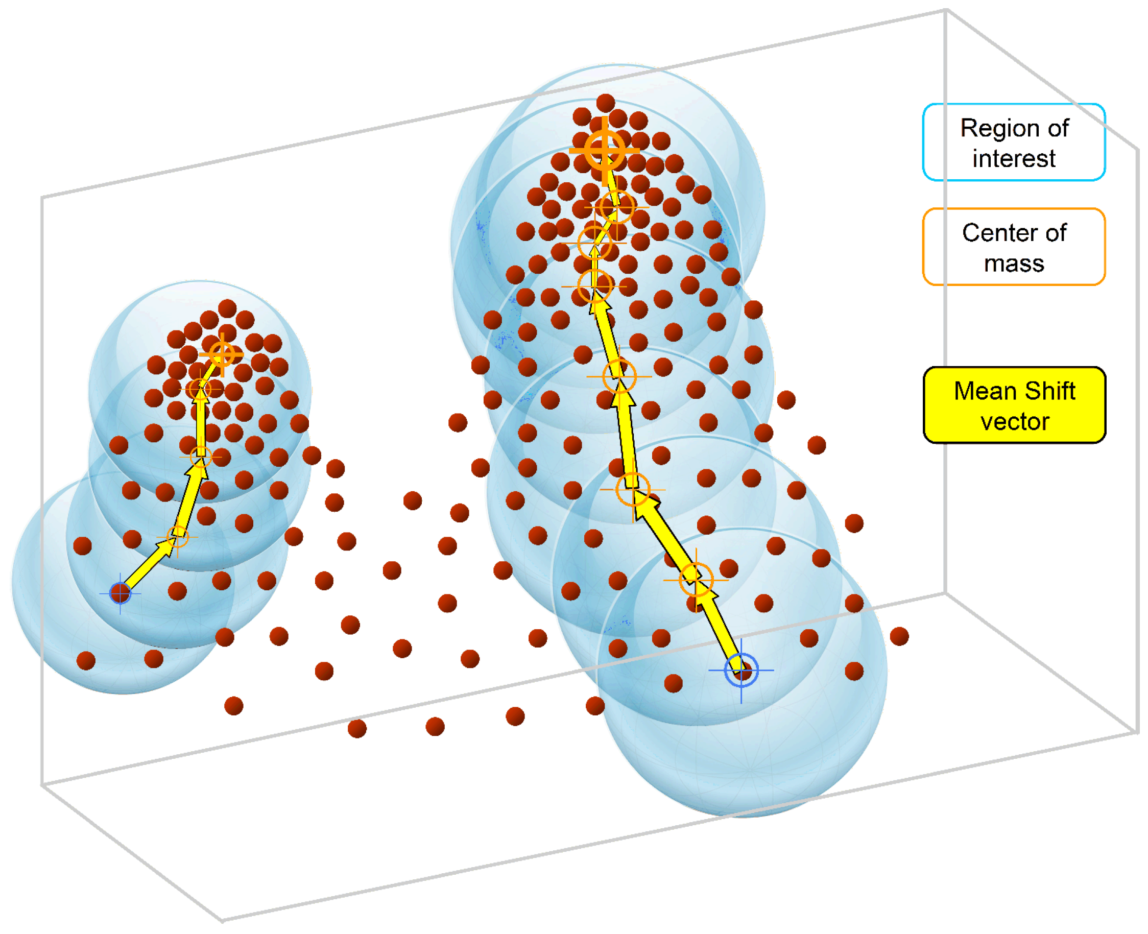
Mean shift is an iterative algorithm using a non-parametric probability density estimator based on the Parzen window kernel function [34]. When used for clustering of unstructured data, the mean shift algorithm aims to move each data point to the densest area in its vicinity until convergence to the local maxima by iteratively performing the shift operation based on kernel density estimation. Figure 3 shows the density estimation procedure with the mean shift vector, which is the difference between the weighted mean and the center of a kernel window (i.e., the region of interest). Given n data points ${\mathbf{x}}_j(j=1,\dots ,n)$ in the d-dimensional space $R^d$, the mean shift vector at point $\mathbf{x}$ is defined as:

$${\mathbf{m}}_{h,G}\left(\mathbf{x}\right)=\frac{\sum _{j=1}^n{\mathbf{x}}_{j}g({∥\frac{\mathbf{x}-{\mathbf{x}}_j}{h}∥}^2)}{\sum _{j=1}^{n}g({∥\frac{\mathbf{x}-{\mathbf{x}}_j}{h}∥}^2)}-\mathbf{x},$$

(1)

where h is the bandwidth parameter and $g(·)$ is called the profile of the kernel $G\left(\mathbf{x}\right)$. By setting:

$$\mathbf{x}(t+1)\leftarrow \mathbf{x}\left(t\right)+{\mathbf{m}}_{h,G}\left[\mathbf{x}\left(t\right)\right],$$

(2)

where t denotes the iteration number, the iterative process converge towards the local maxima. Obviously, a mean shift vector always points toward the direction of the maximum increase in density, and successive vectors can define a path leading to a mode of the estimated density. All data points that have converged to the same mode are grouped together as a cluster. In mean shift theory, a cluster is defined as an area of higher density than the remainder of the dataset, and a dense region in feature space corresponds to a mode (or a local maximum) of the probability density distribution. The ultimate result of the mean shift procedure will associate each point in 3D space with a particular cluster.

For the mean shift algorithm, determination of the kernel bandwidth, the only parameter that needs to be specified, is very critical. It is justified that an adaptive mean shift algorithm automatically calibrating the kernel bandwidth according to local structure information outperforms that using a single bandwidth for the whole feature space. The adaptive mean shift-based clustering scheme presented in our previous study aims to decompose the 3D forest point clouds into segments corresponding to individual tree crowns [26]. It is a two-stage sequential segmentation procedure chain: coarse segmentation (single-scale mean shift-based area partitioning) and fine segmentation (adaptive mean shift-based clustering). The highlight of the adaptive mean shift-based approach is a computationally-efficient method to dynamically calibrate the kernel bandwidth, which is not set to a fixed value or determined as a multi-scale function, but can be varied in a manner that reflects the quantitative information about the local canopy structure. Please refer to [26] for more detailed information about this approach.

The major problem encountered when using mean shift clustering techniques to detect trees is omission and commission errors. The omission errors result from under-segmentation, which implies assigning a LiDAR point cluster to several actual trees, whereas over-segmentation (a single tree segmented into more than one LiDAR clusters) of tree crowns will lead to commission errors. Under-segmentations are more prone to happen than over-segmentations since the tree crown delineation methods based on clustering techniques have the potential of missing field-measured trees: smaller trees are the intermediate and lower height level are unable to be recognized or groups of trees with crowns overlapping each other due to short mutual distances might be treated as one LiDAR segment, in which it is difficult to distinguish and separate individual trees by a clustering-based segmentation technique.

3.2. Concept and Workflow

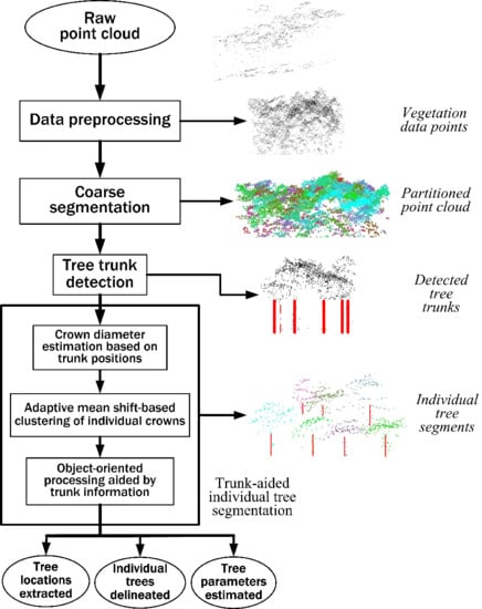
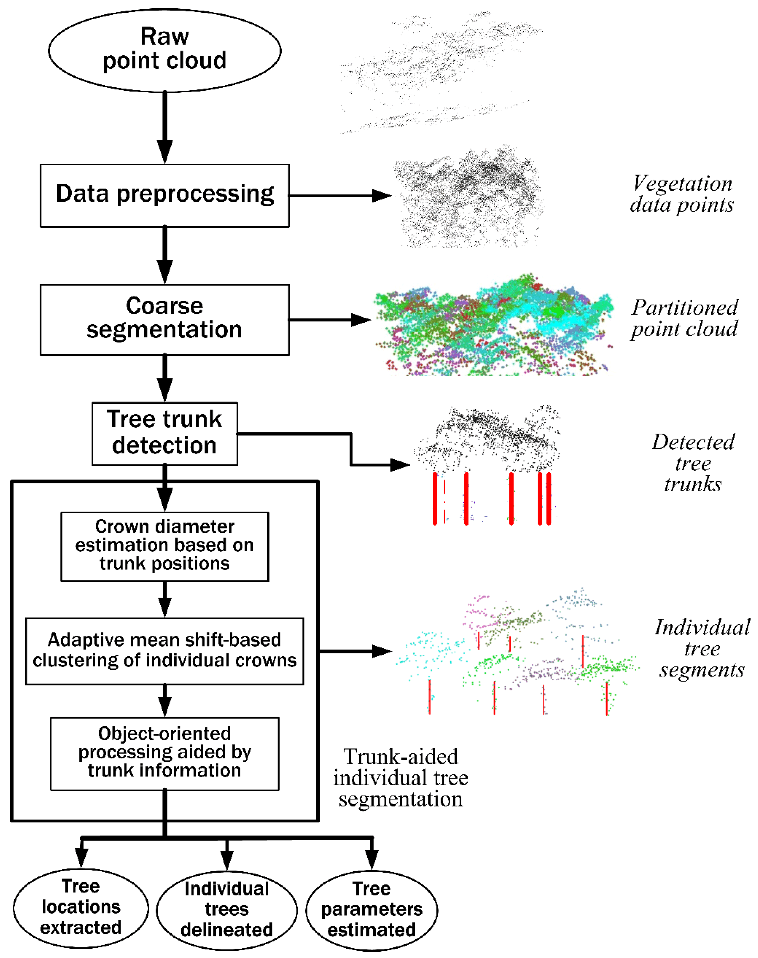
The adaptive mean shift-based clustering technique essentially segments the forest point clouds and delineates individual tree crowns according to the LiDAR point density distribution in 3D space due to the fact that the density of received laser pulses is high at the center of a tree crown and decreases towards the edge of the crown. It performs well in forests or forest layers with regular forms, but its detection accuracy degrades seriously when dealing with forest environments with complex patterns. The main cause is the inadequate tree finding capability inherent in the mean shift-based technique. As a top-down segmentation scheme, it works over the point cloud derived from the laser pulses, mainly sampling the forest canopy structure, but rarely takes into account the LiDAR points under individual tree canopies, which contain structural information reflecting the spatial characteristics of tree trunks. It is advantageous to add a bottom-up strategy into the methodology: the trunk-related information should be utilized to aid in segmentation and delineation of individual trees to improve overall performance.

Taking into account all necessary mathematical processing used in this study, we present a flowchart of methods used in this study, as illustrated in Figure 4, where the ellipses represent data or parameters and the rectangles represent processes or calculations. Each processing step will be described in detail in the following part of this section.

3.3. Data Preprocessing

To focus on individual tree’s delineation and measurement, we need to delete the LiDAR points belonging to the ground surface and the undersized vegetation. Considering that the ground surface is not flat and our proposed approach is based on the relative spacing of each point, we also need to remove the slope effect. First, the raw LiDAR point data were classified into ground points and above-ground points using TerraScan [36]. The aboveground or vegetation points were used in this study. A Digital Terrain Model (DTM) was generated by interpolating the ground points using ordinary kriging, and the vegetation point cloud was normalized by subtracting the DTM height from the raw LiDAR point cloud. After the normalization process, the elevation value (namely the coordinate in the z-dimension) of a point indicates the vertical distance from the ground to the point. Next, data points belonging to non-canopy features in the undersized vegetation strata were cleared. Points whose heights fall in a predefined range $R_{SV}=[0,H_{SV}]$ ($H_{SV}$ is a preset threshold height) were recognized and then removed from the vegetation point cloud. In this study, we deleted all points belonging to the undersized vegetation up to a height value of 1 m from the ground level.

3.4. Coarse Segmentation

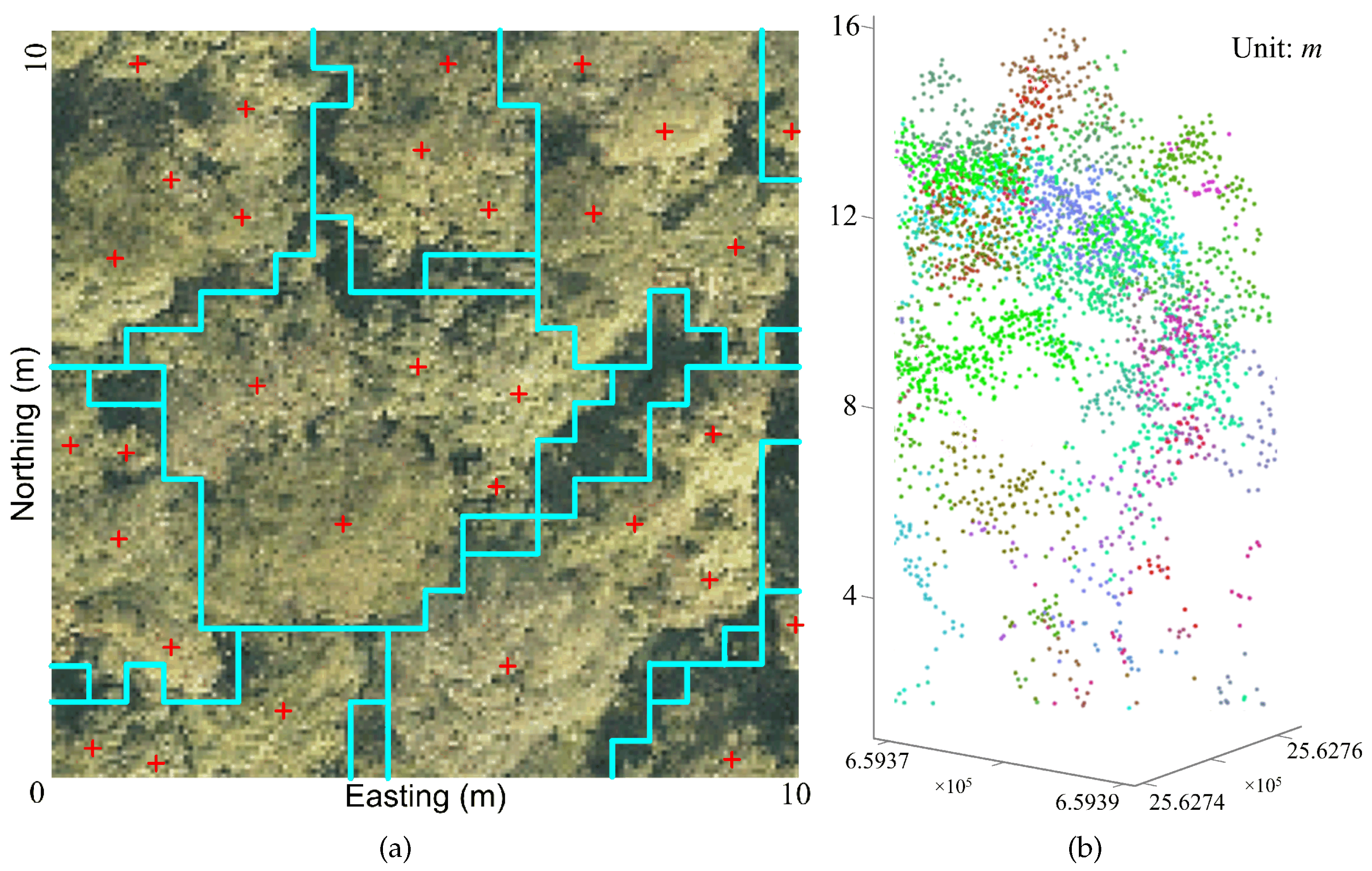
The coarse segmentation aims to partition the 3D space over each forest plot into many small irregular spatial regions, called “partitions” here, each of which contains 3D spatial features representing a single tree or a group of several actual trees. As the sizes of these segments are much smaller compared to that of the original test plot, the subsets of data points in the segments are much easier to handle than the whole dataset contained in a point cloud. For example, when much more complicated analyses and calculations are performed on these segments, which implies more complex mathematics, the total computational load could be reduced to an affordable range. We adopt the single-scale mean shift-based algorithm described in [26] to accomplish coarse segmentation of the LiDAR point cloud. Firstly, a fast mean shift procedure using the simplest kernel function, the uniform kernel, is performed on a part of the dataset (namely the intermediate pulse data) to yield a number of point clusters, each of which reflects the spatial structure of one or more trees. Next, the first pulse data depicting the canopy surfaces are added to expand these clusters to the whole dataset by means of a so-called small square grouping technique. An example of the coarse segmentation results for a small area (10 m × 10 m) selected from a representative subplot is given in Figure 5. For a detailed description of this processing stage, please refer to [26].

3.5. Tree Trunk Detection

The irregular segmented region (a partition of the 3D point cloud data in a forest area of interest) resulting from the coarse segmentation process mentioned above, where obvious under-segmentations occur, usually contains several actual trees. Thus, each individual tree should be further extracted from the partition in the subsequent processing stage. However, only using a crown-based tree delineation method (e.g., the CHM-based watershed segmentation or the mean shift clustering) would result in omission errors (under-detection of trees), or commission errors (over-detection of trees), or both, for the reason that a crown segmentation mostly relies on a detection of tree tops based on local maxima or high densities, but not on a tree trunk detection. A group of trees with LiDAR point patches overlapped cannot be clearly separated by the crown-based segmentation method, whereas their trunks might be isolated from each other using points lying below tree crowns. Apparently, the introduction of the tree trunk detection would help to improve the overall tree detection rate.

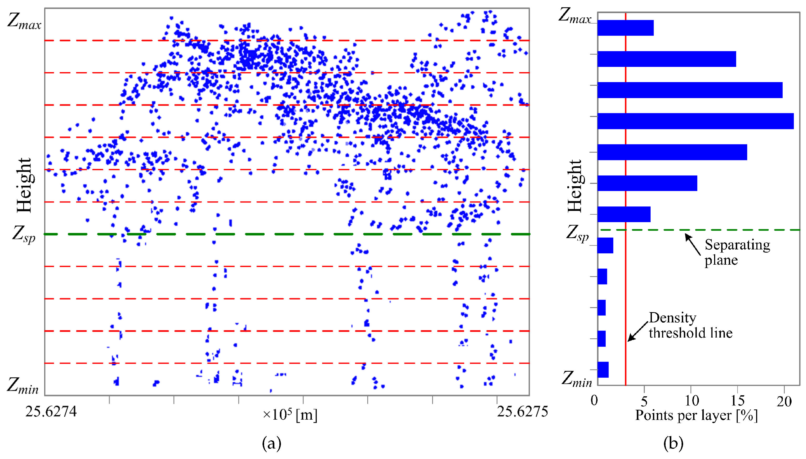
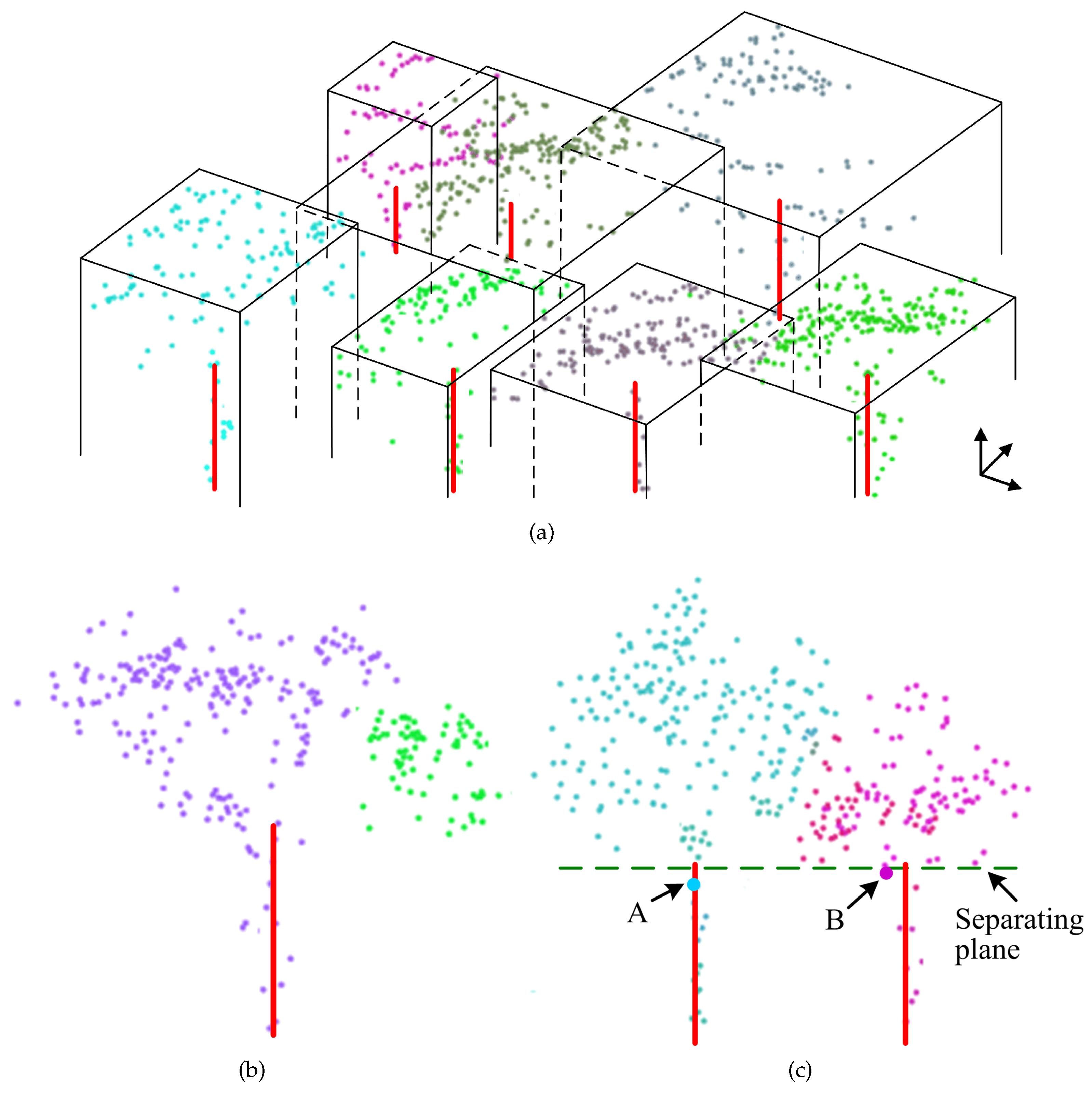
The tree trunk detection adopted in this study works in a two-step algorithm. The first step aims to detach all potential crown points within a specific partition and separate out the trunk section. This goal is achieved by analyzing a vertical histogram of the points within a partition, whose idea is similar to the method presented in [11,37], but easier to implement (Figure 6). Firstly, divide LiDAR points between $Z_{min}$ and $Z_{max}$ ($Z_{min}$ and $Z_{max}$ denote the minimum and maximum elevation values for all points in a partition, respectively) into $N_{lay}$ horizontal layers. Next, generate the histogram of the point distribution along the vertical direction by calculating the number of points per layer and normalizing the results by dividing each of them by the total number of points in the partition. Finally, locate the separating plane that detaches all potential crown points from the trunk section by searching the lowest horizontal layer where the point density exceeds a predefined threshold value: $t{h}_{DPL}$.

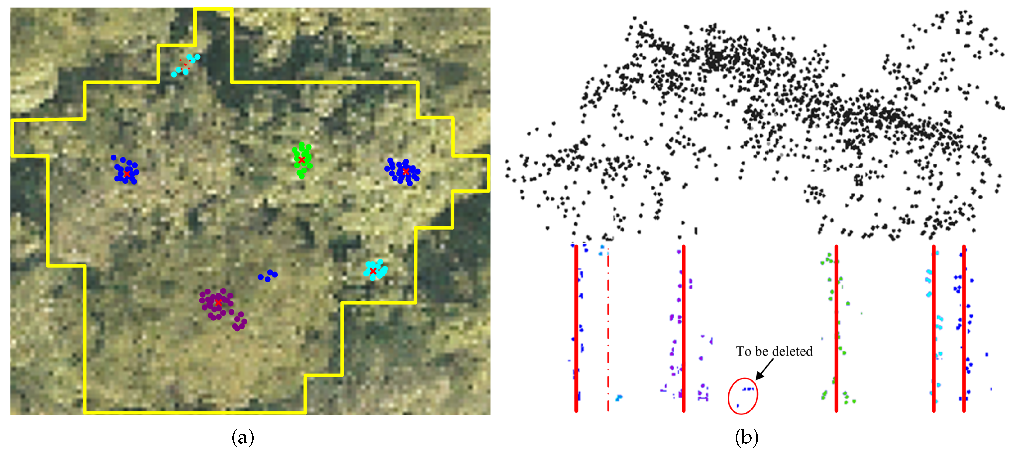
In the second step, the separated trunk points are clustered according to their spatial neighborhood relationships to get an estimation of the number and positions of tree trunks within a specific partition and assign point groups to the estimated trunks. It is assumed that several points that are spatially close together will form a trunk. Isolated points with no or just a few neighbors are assumed to be noise or sparse scrubby vegetation. Due to not knowing the number of trunks a priori, the mean shift algorithm (a non-parametric clustering technique) is also adopted in this step. Prior to cluster analysis, the trunk points are all projected onto a horizontal plane, and a simple mean shift clustering procedure is then performed in the 2D space constituted by these projected points using a flat kernel function:

$$g_u({∥\frac{{\mathbf{x}}^b}{h_b}∥}^2)=\left\{\begin{array}{ccc}1\hfill & & ∥{\mathbf{x}}^b∥\le h_b\hfill \\ 0\hfill & & else,\hfill \end{array}\right.$$

(3)

where ${\mathbf{x}}^b$ denotes the data point in the 2D Euclidean space and $h_b$ is the kernel bandwidth or search window size. Considering that the DBH of the trees in the study area rarely exceeds 0.5 m, we assign a fixed value of 0.75 m (1.5 × 0.5 m) to the bandwidth $h_b$. Any cluster with more than 5 data points is deemed to be a tree trunk; otherwise, it should be treated as noisy data or a segment of lower shrubs or weeds and would be deleted from the trunk points. The approximate trunk position is estimated by finding a cluster’s stationary point. Figure 7 shows the results of tree trunk detection using the above-described mean shift clustering for a typical partition. As can be seen from this example, an obvious commission error, appearing as a falsely-detected trunk, resulted from this tree trunk detection technique.

3.6. Trunk-Aided Mean Shift Clustering for Segmentation of Individual Trees

The aim of this stage is to segment each individual tree from the LiDAR point cloud for a particular forest partition by performing an adaptive mean shift-based clustering analysis with the aid of tree trunk detection results. Although the results contain some errors, they would indicate the general horizontal distribution of trees in a partition, reflecting the basic horizontal structure in a forest area of interest. From this useful information about the local vegetation structure, we can get an estimate of the individual tree crown size, which in turn can be utilized to calibrate the kernel bandwidth of the mean shift procedure adaptively. More importantly, the trunk detection results can provide supplementary information with which the point clusters generated by the adaptive mean shift algorithm are combined to perform the final detection of individual trees. The combinational use of mean shift clustering results and detected tree trunk information in this stage would serve as references against each other to reduce over- and under-segmentations and thus help to improve the overall tree detection accuracy.

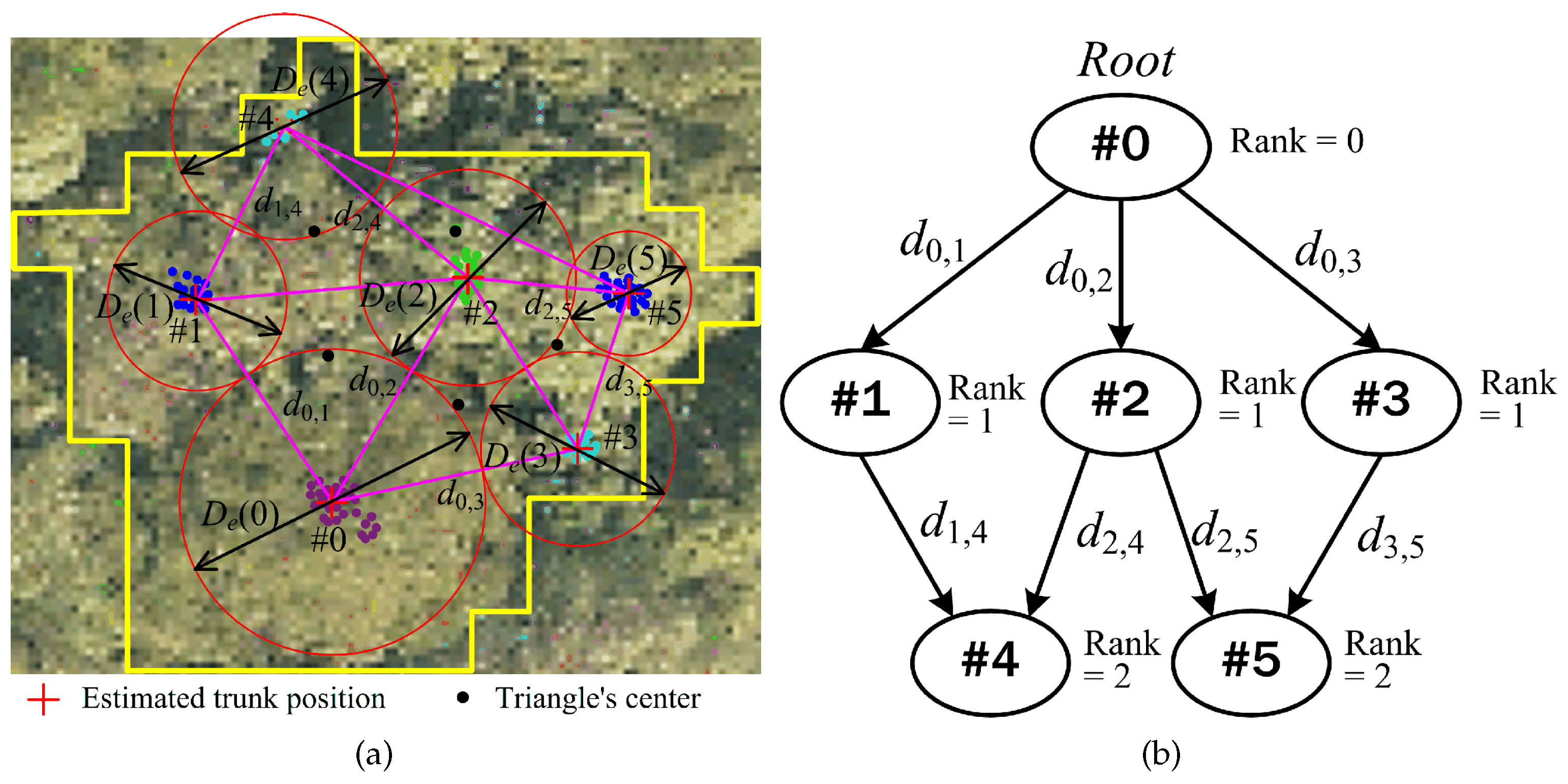
The adaptive mean shift procedure requires the kernel bandwidth to be automatically calibrated according to specific tree crown sizes. However, acquisition of the structural data reflecting the local forest canopy relies on the accurate extraction of individual trees from the LiDAR point clouds. Therefore, this is a chicken and egg debate, and it is very difficult to obtain exact quantitative information about the local spatial structures of the forest canopy prior to complete clustering of individual trees. Yet, it is possible to get rough information about the sizes of individual tree crowns ahead of a tree delineation process, which provides a basis for adaptive determination of the kernel bandwidth. In this study, the data of tree crown widths are roughly estimated based on tree trunk detection results. The estimation algorithm models the individual tree crown as a sphere or a hemisphere, which appears in a 2D circular form when projected onto a horizontal plane, and thus, the estimation problem is reduced to an issue of determining the diameter or radius of these projected circles. The following scheme is applied to achieve the goal of rough estimation of tree crown diameters (Figure 8):

1.

Perform Delaunay triangulation of the 2D point set formed by $N_T$ estimated trunk positions within a partition and calculate each triangle’s center.

2.

Choose the tree trunk with the most LiDAR data points (indicating the highest degree of trueness) as the primary tree (#0 in Figure 8a). Measure the distances from this tree location to centers of all triangles to which it belongs, and take the average of these distances as the radius or half of the diameter of the circle representing the tree’s crown region. In Figure 8a, $D_e\left(0\right)$ is the estimate of the crown diameter for Tree #0.

3.

Use the primary tree as the root to generate a directed acyclic graph (DAG), as illustrated in Figure 8b. Each vertex is assigned a specific rank, the value of which indicates its “distance” to the root. The symbol $d_{i,j}$ appearing beside a directed edge connecting two vertices represents the mutual distance between two neighboring trees with indices of i and j.

4.

For the vertices with the rank value of 1, the crown diameters of their corresponding trees can be roughly determined as follows:

$$D_e\left(k\right)=2d_{0,k}-D_e\left(0\right),k=1,\dots ,K_1,$$

(4)

where $K_1$ is the number of all vertices with a rank of 1.

5.

For other vertices, the rank values of which exceed 1, use the following formula to estimate their crown diameters:

$$D_e\left(k\right)=\frac{1}{N_k}\sum _{i=1}^{N_k}2d_{k_i,k}-D_e\left(k_i\right),k=K_1+1,\dots ,N_T-1,$$

(5)

where $N_k$ is the total number of directed edges ending at Vertex #k and $k_i$ is the index of each directed edge’s starting vertex.

Next, an adaptive mean shift-based clustering analysis is performed on the dataset constituted by all separated tree crown points within a partition. A truncated, multivariate Gaussian function is adopted as the kernel or window in this stage. Each data point in the feature space will be associated with a specific kernel function, which is characterized by the adaptable kernel bandwidth (or window size), which can be varied according to the estimated tree crown diameter. Map the point onto the horizontal plane in Figure 8a to see in which projected circular region it falls. If this point is not in any circle or belongs to two or more circles at the same time, assign the nearest circle to it. Assume the corresponding tree circle has the index number of k, and then, determine the variable kernel bandwidth as follows:

$$h_{var}=D_e\left(k\right),$$

(6)

where $h_{var}$ is the variable kernel bandwidth. Please refer to [26] for more detailed information about this adaptive mean shift algorithm.

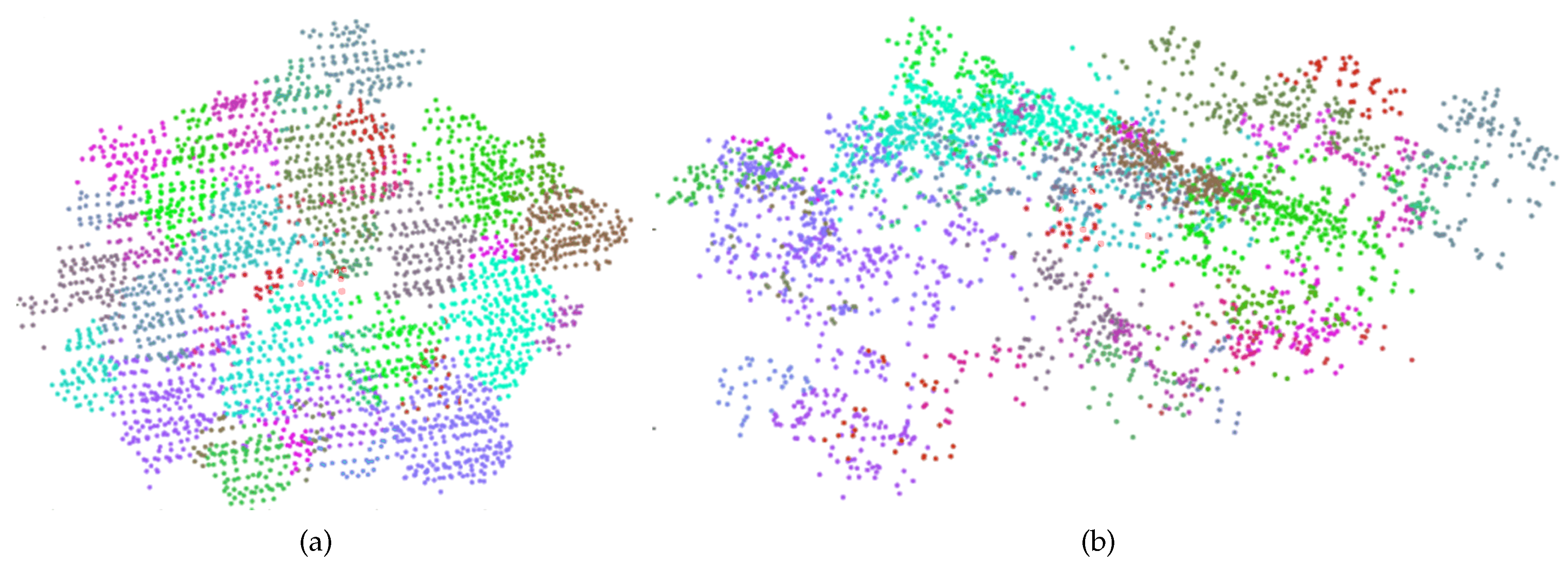
An example of clustering results of the above-described adaptive mean shift algorithm is shown in Figure 9. The major weakness of this clustering algorithm is that it tends to merge nearby trees or smaller trees into one single tree. Owing to the inability to detect suppressed trees or the difficulty in discriminating two overlapping tree crowns or oversized kernel bandwidths, omission errors (or under-segmentations) are very likely to happen in the clustering results (Figure 10a,b). Besides, commission errors can also occur in the segmentation results of the adaptive mean shift-based clustering due to a loose canopy structure or because the derived kernel bandwidth somewhere is too small relative to its local canopy structure (Figure 10c).

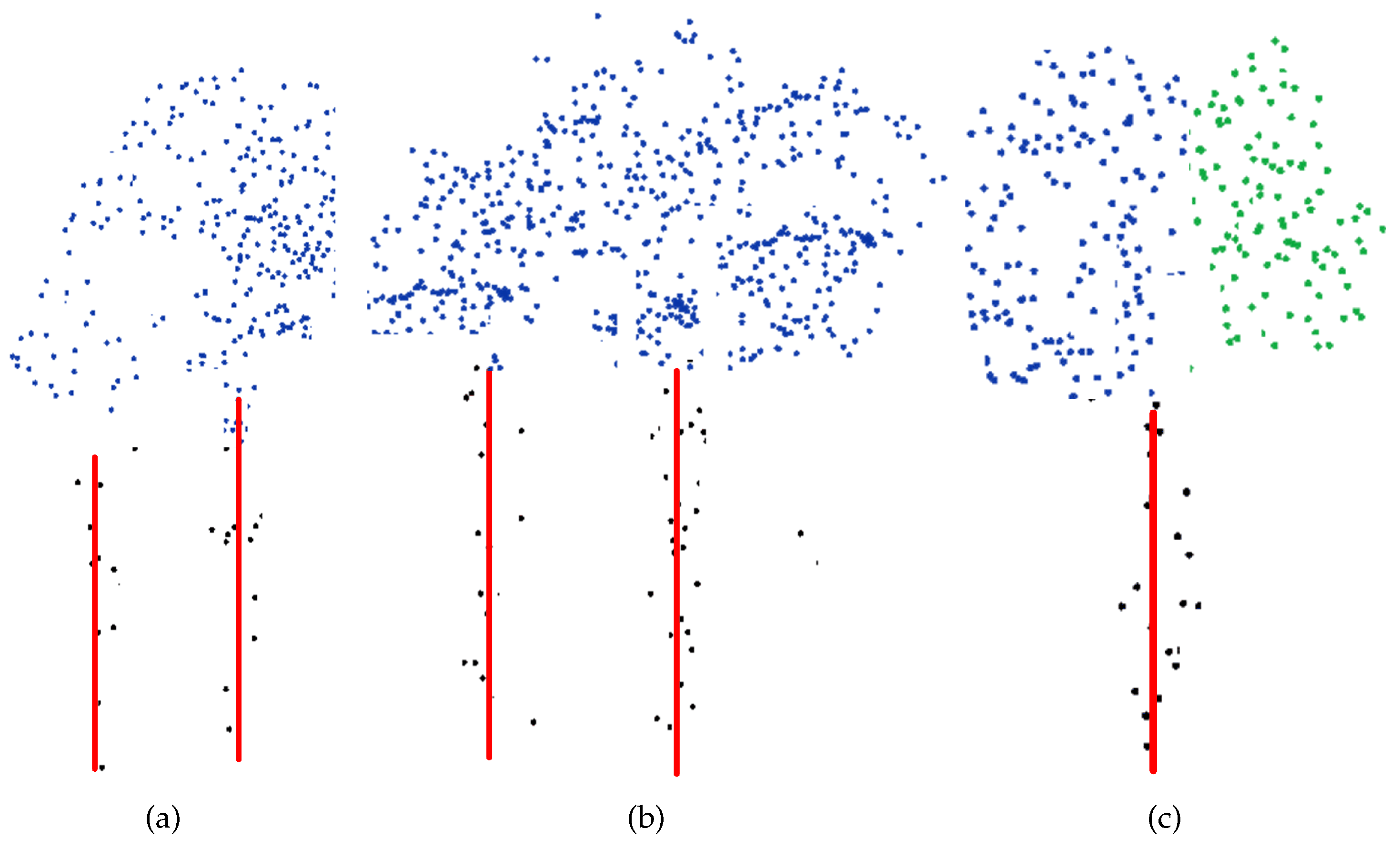
These problems originate from the spatial information contained in the dataset used by the algorithm, which mainly reflects the forest canopy’s structural characteristics. In order to tackle the weaknesses of the adaptive mean shift-based segmentation, additional information should be introduced to perform further analysis of LiDAR segments in the crown section. In this study, we utilize the tree trunk information to aid in the ultimate object-oriented processing, where the combinational use of trunk detection results and clustering results of crown points implies mutual reference based on which final decisions could be made to identify and delineate individual trees. Such a process aims to improve the overall detection accuracy, especially for structurally complex forests where most of the trees overlap. A detailed description of this technique is given in the following:

1.

Check the tree trunk detection results with respect to crown point segments. As the trunk area might not be reliably separated from the crown points and thus there could be errors in trunk detection, it makes sense to use the crown point cloud as a reference to verify the results of tree trunk detection. If there is no crown segment in the region right over an estimated tree trunk, which is defined as a circle with a radius of 0.5 m centered on the trunk’s approximate position, the trunk is considered as a dead tree or a low-growing plant and would be deleted from the trunk section. Any trunk cluster whose lowest point has an elevation value of more than $(Z_{sp}+Z_{min})/2$ would be deemed to be a segment from the canopy and should be ignored. If a point cluster in the trunk section is composed of disjointed segments whose maximum elevation difference exceeds $(Z_{sp}-Z_{min})/2$ (as depicted by the dashed line in Figure 7b), we would regard it as a fictitious tree trunk.

2.

Link the point clusters in the crown section to the validated stem points in the trunk section. Firstly, determine the axis-aligned bounding box for each crown segment. Then, check to see if there are detected tree trunks in these bounding boxes. In case there is only one trunk in a bounding box, associate the trunk points with the crown points contained in the box and combine them to delineate the whole structure for an individual tree (Figure 11a).

3.

If a segment in the crown section is not linked to any trunk points, it would be treated as a part of a tree crown. Merge this segment into the adjacent tree nearest to it. An example of point cloud merging is illustrated in Figure 11b. According to this rule, the right segment rendered in green color, with no trunk under it, would be incorporated into a larger segment on the left.

4.

If there is more than one trunk contained in a bounding box, the point cloud in this box should be split into several parts, the exact number of which depends on the number of identified tree trunks. To achieve this goal, crown points are classified sequentially from bottom to top and will be allocated to the corresponding tree trunks. Each tree crown is built up concurrently beginning from its seed point, which is defined by the highest point of each identified trunk, by including nearby points and excluding points of other crowns based on their relative spacing. In the crown growing process, the spatial distances between the unclassified points and the semi-grown crown points are calculated. A point will be allocated to a target tree crown if the spatial distance to one of the points from that crown is the shortest. This minimum spacing rule-based tree crown growing process is illustrated in Figure 11c.

3.7. Tree-Based Parameter Estimation

Once individual trees are accurately identified, tree structural attributes such as tree height, crown width and height and the number density of trees can be directly derived from the segmented points. From these parameters, other forest parameters, such as DBH, Crown Base Height (CBH), basal area, LAI, wood volume, biomass and species type, could be estimated from allometric equations. As our main objective was to develop a methodology to accurately segment individual trees from LiDAR data, we focus on two parameters for which we had in situ measured values from a ground survey, namely tree height and crown diameter.

The highest point among the segmented points for each tree is considered as the tree top, and the distance to the tree top from the ground is regarded as the height of that tree. Tree heights are commonly underestimated in LiDAR studies because the transmitted laser pulses may miss the actual tree top [38]. Increasing the spatial density of LiDAR points provides a better chance of hitting the tree top, resulting in higher accuracy. The crown diameter is defined as the average of two values of crown widths measured along two perpendicular directions from the location of the tree trunk. The method to estimate individual tree crown diameter presented in [7] is adopted in this study. Firstly, project the points from the topmost crown into the x-y plane, and extract perpendicular profiles of them centered on the tree trunk. Then, fit a fourth-degree polynomial on each profile, and find critical points of the fitted function around the center (namely the trunk position). Next, calculate crown width on each profile as the distance between critical points on each side of the center. Finally, the value for a crown diameter is computed as the average of the crown widths along the two directions or profile.

3.8. Implementation

A prototype system for 3D forest point cloud data processing was developed using the C/C++ programming language based on the Point Cloud Library (PCL) (Open Perception: Menlo Park, CA, USA), an open-source library of algorithms for point cloud processing tasks and 3D geometry processing, to verify our proposed approach, while the calibration and validation of the approach was performed in MATLAB (The MathWorks: Natick, MA, USA). Generic techniques for classification, filtering, segmentation, modeling and visualization of 3D point clouds were implemented with the methods and classes contained in PCL’s modules. The iterative computing procedures for the mean shift-based clustering were accomplished by calling a C++ wrapper that implements a standard mean shift algorithm. In particular, the approach-specific algorithms, such as tree trunk detection, kernel calibration and object-oriented post-processing, were implemented from scratch.

4. Results

4.1. Individual Tree Detection

The 3D segmentation of individual trees was validated by comparing field measurements with LiDAR segments. A LiDAR data segment was linked with a reference tree provided that: (i) the distance to the reference tree was smaller than 60% of the mean tree distance within the subplot; and (ii) the difference between the derived tree height and the height of the reference tree was smaller than 15% of the top height of the subplot. The results of tree detection for more than 1700 trees in 10 sample plots (i.e., 20 test subplots) are presented in

Table 1. Results of individual tree detection for all trees in 20 test subplots.

Subplot ID	Reference Trees	Detected Trees	TP 1	FP 1	FN 1	Recall (r)	Precision (p)
DHS0101	96	93	88	5	8	0.917	0.946
DHS0102	101	96	91	6	11	0.900	0.948
DHS0201	111	106	98	9	13	0.883	0.924
DHS0202	153	145	133	13	21	0.869	0.917
DHS0301	128	122	112	11	16	0.875	0.918
DHS0302	98	96	91	6	8	0.928	0.948
DHS0401	87	85	80	5	7	0.920	0.941
DHS0402	71	71	68	3	3	0.958	0.958
DHS0501	68	68	65	3	3	0.956	0.956
DHS0502	74	73	69	4	5	0.935	0.932
DHS0601	116	113	103	10	13	0.888	0.916
DHS0602	105	104	96	8	9	0.914	0.923
DHS0701	71	70	67	3	4	0.944	0.957
DHS0702	67	68	64	4	3	0.955	0.941
DHS0801	112	108	98	10	14	0.875	0.907
DHS0802	75	76	71	5	4	0.947	0.934
DHS0901	78	76	73	3	5	0.936	0.960
DHS0902	111	106	97	9	14	0.874	0.915
DHS1001	28	28	28	0	0	1.000	1.000
DHS1002	29	29	29	0	0	1.000	1.000
Overall	1779	1733	1621	117	161	0.911	0.935

¹ TP, True Positive; FP, False Positive; FN, false negative.

. To evaluate the accuracy of the detection results quantitatively, two indices (“recall” and “precision”, indicating the tree detection rate and the correctness of detected trees, respectively) based on three types of segmentation results were adopted in this study. The “recall” (r) and “precision” (p) are defined as follows [39]:

$$\begin{array}{c}\hfill r=\frac{TP}{TP+FN},\end{array}$$

(7)

$$\begin{array}{c}\hfill p=\frac{TP}{TP+FP},\end{array}$$

(8)

where TP (True Positive) is the number of individual trees that were segmented correctly, FN (False Negative) represents the number of under-segmentations where a tree was not detected and assigned to a nearby tree and FP (False Positive) indicates the number of over-segmentations where a point cluster was segmented as a tree that did not actually exist. It is worth noting that the “recall” is inversely related to omission error, and the “precision” is inversely related to commission error.

4.2. Tree-Based Parameters

Having matched the segmented LiDAR data with the field survey data, we could carry out a performance evaluation of the tree-based parameter estimation. Two tree structural parameters (tree heights and crown diameters) derived from the LiDAR data were validated with field-measured tree heights and crown diameters. Only correctly-detected trees were used; that is, falsely-detected trees and missed trees were not counted. We used all correctly-detected trees (nearly 900 trees) in 10 test subplots with the IDs DHS0101, DHS0102, DHS0201, DHS0202, DHS0301, DHS0302, DHS0401, DHS0402, DHS0501 and DHS0502 in this experiment. The statistics for the two LiDAR estimated parameters are summarized in the following: the mean relative errors between estimates and ground truth values for tree height and crown diameter were −2.21% and 0.65%, respectively, and the standard deviations or the relative RMS (Root Mean Square) errors in the estimates were 5.85% and 21.92%, respectively. A negative value of the mean error means an underestimation, while a positive value implies an overestimation. Figure 12 correlates the LiDAR-derived and field-measured tree heights and crown widths for the correctly-detected trees. The scatterplots of LiDAR-estimated vs. field-measured tree heights and crown diameters for all correctly-detected trees contained in 10 subplots are shown in Figure 12a,b, respectively. A simple linear regression was used to fit the lines (marked in red) to each dataset. For tree height estimation, the slope of the linear regressions almost equaled one, and the value of $R^2$ was 0.9863. Yet, for the estimates of crown diameter, the correlation result was relatively weak with $R^2$ = 0.8584.

4.3. Tree Position Differences

In this study, the stationary point of a cluster formed by horizontally-projected LiDAR points in the trunk section (or the cluster’s center of gravity) was determined as the approximate position of the tree corresponding to this cluster. This processing was essentially to find the intersections of the detected tree trunks with the ground. Figure 13a shows the histogram of tree positioning errors (namely, the distances between the estimates and the field-measured values of the correctly-detected trees’ horizontal coordinates) using our proposed trunk-aided mean shift approach. As a contrast, the histogram generated by the adaptive mean shift approach presented in [26] is given in Figure 13b.

Table 2. Positioning accuracy comparison for 895 correctly-detected trees.

Method	Mean Difference (m)	Standard Deviation (m)
Proposed trunk-aided mean shift clustering	0.562	0.424
Adaptive mean shift clustering in [26]	0.851	0.653

lists the statistics of tree positioning errors for the two approaches mentioned above.

5. Discussion

This paper addresses the methods of airborne LiDAR-based remote sensing for individual tree-level forest inventory in which the detection of individual trees is one of the key issues. The mean shift-based clustering technique needs no seed points for initialization and works fully in three dimensions, and so, it is becoming a promising technique of producing relatively high accuracy by detecting more small trees in the lower and intermediate forest layer than other methods. Mean shift’s applications in individual tree detection using LiDAR data were explored in [15,24,25]. In our previous work, we developed an adaptive mean shift-based clustering scheme, which automatically calibrated the kernel bandwidth to the local spatial structure of the forest canopy [26]. The approach of tree trunk detection-aided mean shift clustering presented in this paper goes one step further than existing schemes by utilizing additional information below the tree crowns. To assess the overall performance of our proposed trunk-aided mean shift clustering approach, we compare the detection results of this approach with those obtained by several different existing approaches.

Firstly, the overall tree detection rates for trees located in different forest stories within six test subplots with IDs of DHS0101, DHS0102, DHS0201, DHS0202, DHS0301 and DHS0302 were compared between two mean shift-based clustering schemes (the proposed trunk-aided method in this study vs. the adaptive method presented in our previous study [26]) to verify whether the trunk detection process works. As illustrated in

Table 3. Accuracy assessment for different tree classes in six subplots: the proposed trunk-aided mean shift method in this study vs. the adaptive mean shift method presented in our previous study.

Class of Trees	Reference Trees	Proposed Trunk-Aided Method				Adaptive Method Presented in [26]
		Detected Trees	TP	Recall	Precision	Detected Trees	TP	Recall	Precision
Dominant trees	234	232	230	0.983	0.991	232	230	0.983	0.991
Codominant trees	209	207	203	0.976	0.981	205	201	0.962	0.980
Intermediate trees	151	141	120	0.795	0.851	138	117	0.775	0.848
Suppressed trees	93	78	60	0.618	0.769	67	45	0.484	0.672
Total	687	658	613	0.892	0.932	642	593	0.863	0.924

, although the detection rates of both methods decrease with dominance position, the trunk-aided method shows clearly higher accuracies than the other one for each forest story, especially for suppressed trees in the understory: nearly 13% more suppressed trees can be detected. This performance improvement is achieved by significantly reducing both the omission error (indicated by the FN count, reduced from 48 to 33) and commission errors (indicated by the FP count, reduced from 22 to 18). Furthermore, our proposed approach is compared to some representative approaches in terms of the accuracies of individual tree detection, as shown in

Table 4. Comparison of overall detection accuracy among different approaches. CHM, Canopy Height Model.

Method	Detected Trees	TP Count	Recall	Precision	F-Score
Proposed trunk-aided mean shift algorithm	1733	1621	0.911	0.935	0.923
Adaptive mean shift algorithm in [26]	1674	1532	0.861	0.915	0.887
Mean shift algorithm in [15]	1589	1425	0.801	0.897	0.846
Region growing in [2]	1531	1343	0.755	0.877	0.811
k-means clustering in [19]	1548	1367	0.768	0.883	0.821
CHM-based method in [40]	1408	1191	0.669	0.846	0.747

. In addition to the indicators of “recall” (r) and “precision” (p), the “F-score” ($F=2\times (r\times p)/(r+p)$) is used in the comparison to evaluate the overall detection accuracy. Except the adaptive mean shift-based clustering algorithm presented in [26], the approaches chosen for this accuracy comparison include: a region growing approach presented in [2], a k-means clustering approach presented in [19], a mean shift-based approach described in [15] and a CHM-based approach adopted in [40]. For more detailed descriptions about these individual tree detection approaches, please refer to [26]. From the data listed in Table 4, the proposed trunk-aided mean shift approach has the highest tree detection rates among all approaches used in this comparative experiment, and the accuracy improvement of our previous work (the adaptive mean shift-based clustering algorithm presented in [26]) by applying the tree trunk detection strategy is noticeable: the overall detection accuracy in terms of “recall” is increased by 5%.

In order to compare the overall tree detection performance among different approaches in a statistically-rigorous fashion, the statistical significance of differences in detection accuracy was evaluated in terms of the overall accuracy metric: the “F-score”. As there is no parametric test suitable for this task, a Monte Carlo permutation test presented by [41] was adopted here to determine the statistical significance of the difference between two F-scores. In this test, 999 permutations were generated, and for each permutation, the pairings of the actual trees with the predicted trees defined by two detection approaches were randomly shuffled; the F-scores were recomputed; and the difference between the two derived F-scores was estimated. Assuming the common situation in which a two-sided test (the null hypothesis that there is no significant difference between the two F-scores) at the five percent level of significance is undertaken, the difference between two F-scores derived with the same datasets would be regarded as being statistically significant if the computed proportion was less than 0.05. The results of a selection of pairwise comparisons are summarized in

Table 5. Pairwise comparisons of the accuracy statements based on the F-scores derived for different tree detections. All tests shown were two-sided and the 5% level of significance selected.

Detection 1	Detection 2	${\mathit{F}}_1$	${\mathit{F}}_2$	${\mathit{F}}_1-{\mathit{F}}_2$	Significant?
Trunk-aided mean shift	Adaptive mean shift	0.923	0.887	0.036	Yes, 2%
Trunk-aided mean shift	Fixed-bandwidth mean shift	0.923	0.846	0.077	Yes, 1%
Trunk-aided mean shift	Region growing	0.923	0.811	0.112	Yes, 0.5%
Trunk-aided mean shift	k-means clustering	0.923	0.821	0.102	Yes, 0.5%
Trunk-aided mean shift	CHM-based method	0.923	0.747	0.176	Yes, 0.3%
Adaptive mean shift	Fixed-bandwidth mean shift	0.887	0.846	0.041	Yes, 2%
Fixed-bandwidth mean shift	Region growing	0.846	0.811	0.035	Yes, 2%

.

Obviously, the proposed trunk-aided mean shift approach accounts for an accuracy improvement of the overall tree detection rate (see Table 4 and Table 5). Such an improvement of the tree detection performance could be expected since in many forest stands, neighboring trees with crowns overlapping each other do not appear as two distinct clusters in the point clouds, but their trunks can be clearly separated for the simple reason that the point structure of trunks is less ambiguous compared with crown shapes that are partially merged. 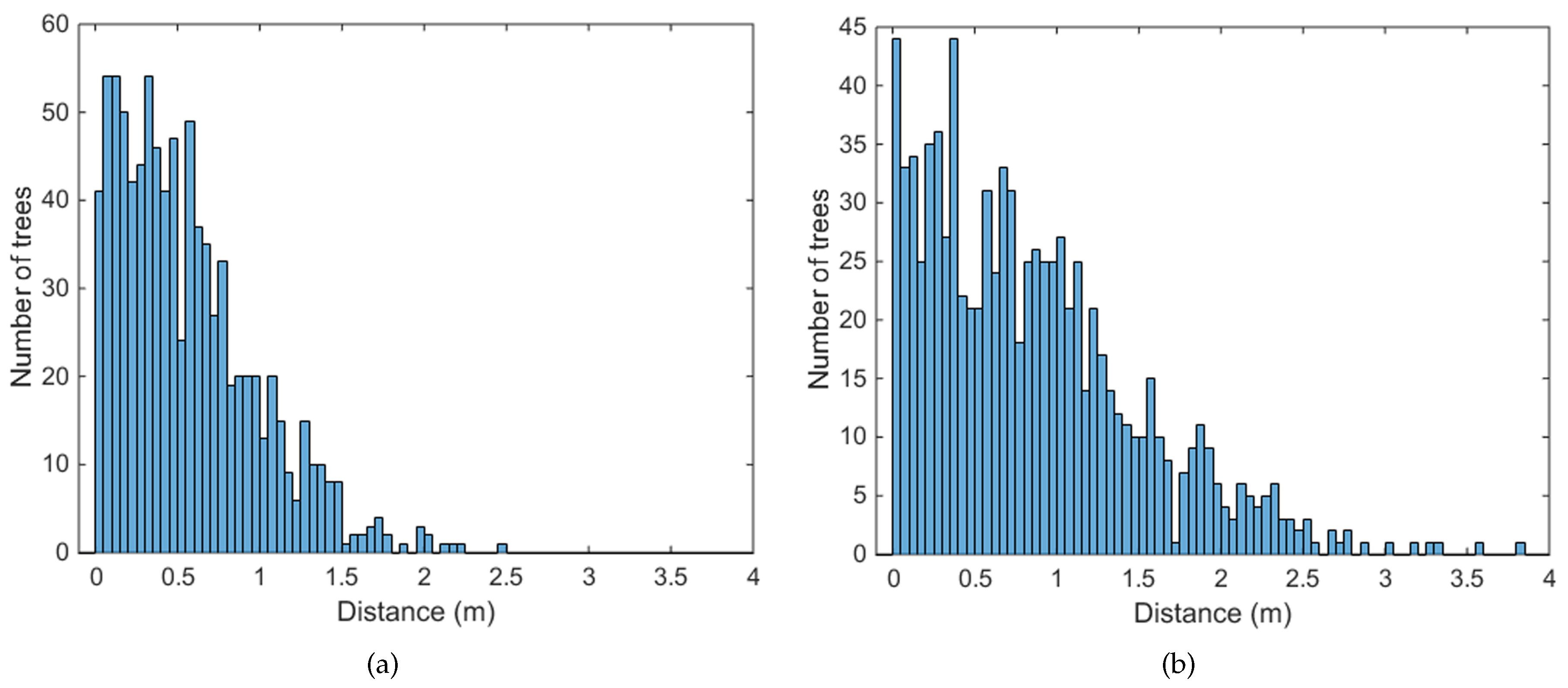The refinement of the detection rate is especially apparent for the intermediate and suppressed trees, as shown in Table 3. Another strength of the proposed techniques is that the accuracy in tree positioning is significantly improved (see Table 2). This is mainly due to the fact that the intersection of the detected tree trunk with the ground must be more precise than the approximate tree position derived from the stationary point of a data cluster.

The major limitation or the biggest uncertainty of the proposed approach is that not all tree trunks can be correctly detected. The performance of trunk extraction depends on the LiDAR point density and the forest type [11,28]. The trunk detection works successfully, if there are enough laser hits at the trunk and if the trunk area can be reliably separated from the crown points. Otherwise, when reflections of the laser beam in the trunk area are rare and trunk points cannot be clearly clustered, or when many suppressed or small trees are located below the taller trees, trunk detection would fail, and thus, the achieved improvement of the overall tree detection would be low. The second limitation, not just for this approach, but a common problem for individual tree-level forest inventory systems using aerial remote sensing technologies, is the under-segmentation issue [27]: still, 8.9% of trees cannot be detected correctly in the studied forest plots using our approach. The reason is that laser beams are less likely to penetrate the forest canopy and hit suppressed trees, and this will disable the algorithms to extract the tree crowns or trunks in the segmentation stage. Other drawbacks of the approach are caused by the simplified removal of ground-covering vegetation, the simplified technique of determining the separating plane between the trunk and crown areas and insufficient rules to decide if a point group represents a trunk. Due to these drawbacks, a detected tree trunk may be fictitious, or the crown points belonging to a partition cannot be separated with respect to the detected trunks.

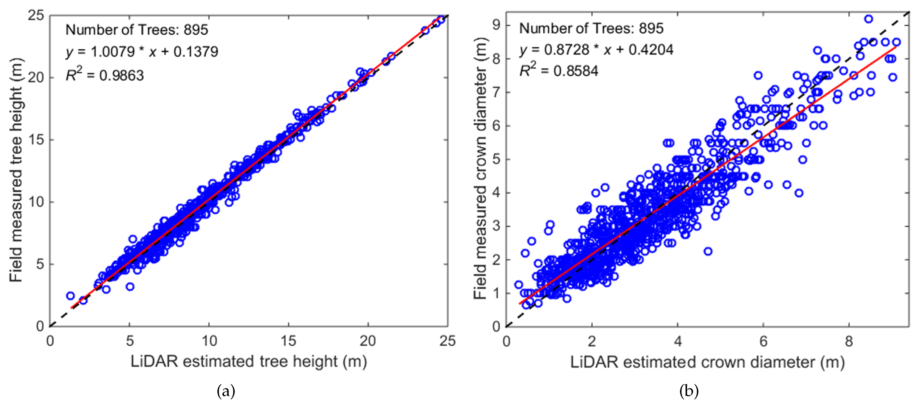
Performance evaluation of the tree-based structural parameter estimation can be conducted by statistics calculation and regression analysis. The linear fit for the tree height’s scatterplots reveals a slope nearly equal to one (1.0079) and an offset of 0.1379; this manifests a systematic underestimation of tree heights by the LiDAR data, which is consistent with other similar studies [2,15,19,40], as shown in

Table 6. Accuracy comparisons of tree height and crown diameter estimation among different methods.

Method	Tree Height		Crown Diameter
	Mean Relative Error	Relative RMS Error	Mean Relative Error	Relative RMS Error
Proposed trunk-aided mean shift	−2.21%	5.85%	0.65%	21.92%
Adaptive mean shift in [26]	−2.45%	7.17%	0.93%	33.59%
Mean shift in [15]	−2.84%	8.52%	0.92%	39.47%
Region growing in [2]	−2.92%	8.16%	1.37%	42.75%
k-means clustering in [19]	−2.68%	7.83%	0.96%	36.98%
CHM-based method in [40]	−3.17%	9.76%	1.84%	50.72%

. The underestimates were due to the lower probability that an emitted laser pulse will strike the top of a tree rather than elsewhere on the tree crown. Additionally, each laser beam will penetrate tree foliage to some degree before being reflected back to the sensor. The regression analysis results also indicate that the average crown width is less accurately estimated, with a relative RMS error of 21.92%, than the tree height. Most of the variance associated with crown diameter can be attributed to the difference between overlapping and non-overlapping crown widths since LiDAR can only measure non-overlapping tree crowns (the algorithm for crown diameter estimation on the segmented LiDAR points aims at measuring the non-overlapping crowns), while the field measurements consider tree crowns to their full extent and therefore measured overlapping crown widths. Another portion of the variance for crown diameter can also be attributed to uncertainties in the ground surveys themselves because of random measurement errors induced by terrain conditions, measuring apparatus or field personnel. Compared with other approaches presented in the above-mentioned literature, the proposed trunk-aided mean shift approach could achieve higher accuracy in estimation of tree heights and crown diameters for individual trees (see Table 6). This is mainly due to the more precise crown characterization ability offered by the proposed approach than other ones.

Further accuracy refinements for individual tree detection and tree parameter estimation could be achieved by increasing the average LiDAR point density, which refers to the nominal value influenced by the laser pulse repetition frequency, flight pattern, flying height, flying speed and strip overlap [2,11]. The common means to increase the LiDAR point density include reducing the flying speed, increasing the overlapping of laser strips, accelerating the emission of laser pulses, etc. Alternately, the overall point density could be increased by optimizing the flight pattern; for instance, flight lines can be surveyed twice or even more [28]. Apparently, a laser scanner with a higher point density could provide sufficient data points reflected from the tree trunk and thereby optimize the trunk detection accuracy. Furthermore, a higher LiDAR point density increases the chance of a laser pulse return from the highest point in each tree canopy, thus reducing underestimation of tree heights. Moreover, further improvements of individual segmentation processes are possible by more sophisticated post-processing of the clustering results based on shape-related rules or using a priori knowledge about the forest. For instance, LiDAR clusters could be tested with respect to closeness. Furthermore, a cluster could not be accepted if its size exceeds tolerances about the tree shape. These issues will be addressed in our future research. Considering there are some limitations for tree segmentation based solely on LiDAR measurements, we also plan to use the proposed techniques in conjunction with aerial imagery, which provides better planform geometry and color (spectral) information, to further improve individual tree segmentation.

6. Conclusions

In this study, we developed an adaptive mean shift-based approach aided by the tree trunk detection technique to segment individual trees and estimate tree structural parameters from 3D point clouds. It is an improved clustering scheme incorporating a bottom-up segmentation strategy, which has the potential to be successfully applied to structurally complex forests. By applying the proposed approach to LiDAR data acquired in a multi-layered evergreen mixed forest located in South China and comparing it with existing point-based approaches in terms of tree detection rates and biophysical parameter estimation accuracies, we have shown that the combination of adaptive mean shift clustering and detected tree trunk information can lead to a significant performance improvement in individual tree-level forest measurement. This is mainly due to the more precise tree characterization ability inherent in the proposed approach by detecting more vegetation features in the mode space that are hard to discriminate by conventional clustering techniques. This study demonstrates the ability of our proposed approach to offer full 3D forest structure characterization in both vertical and horizontal dimensions, which creates a platform to develop new LiDAR remote sensing techniques at the individual tree level to quantify the wood volume, biomass and even biological diversity of forests. By including high-resolution imagery along with the LiDAR point-cloud data, the object-oriented segmentation at the species level allows for a complete characterization of forests from remote sensing platforms.