Band Priority Index: A Feature Selection Framework for Hyperspectral Imagery

Abstract

Hyperspectral Band Selection (BS) aims to select a few informative and distinctive bands to represent the whole image cube. In this paper, an unsupervised BS framework named the band priority index (BPI) is proposed. The basic idea of BPI is to find the bands with large amounts of information and low correlation. Sequential forward search (SFS) is used to avoid an exhaustive search, and the objective function of BPI consist of two parts: the information metric and the correlation metric. We proposed a new band correlation metric, namely, the joint correlation coefficient (JCC), to estimate the joint correlation between a single band and multiple bands. JCC uses the angle between a band and the hyperplane determined by a band set to evaluate the correlation between them. To estimate the amount of information, the variance and entropy are used as the information metric for BPI, respectively. Since BPI is a framework for BS, other information metrics and different mathematic functions of the angle can also be used in the model, which means there are various implementations of BPI. The BPI-based methods have the advantages as follows: (1) The selected bands are informative and distinctive. (2) The BPI-based methods usually have good computational efficiencies. (3) These methods have the potential to determine the number of bands to be selected. The experimental results on different real hyperspectral datasets demonstrate that the BPI-based methods are highly efficient and accurate BS methods.

1. Introduction

Hyperspectral images contain hundreds of bands with a fine resolution, e.g., 0.01 $\mathsf{\mu }$m, which makes it possible to reduce overlap between classes, and, therefore, enhances the potential to discriminate subtle spectral difference [1,2]. However, the high dimensionality of dataset also brings several problems, such as heavy computational burden and storage cost. In addition, the high resolution of the spectrum makes the bands highly correlated. Therefore, to process data effectively, dimensionality reduction (DR) is important and necessary. Dimensionality reduction techniques can be broadly split into two categories: feature extraction and feature selection (i.e., band selection) [3,4]. Feature extraction reduces the data dimensionality by extracting a set of new features from the original ones through some function mapping. For instance, Principle Component Analysis (PCA) [5] is one of the well-known feature extraction methods, and other feature extraction methods include Nonnegative Matrix Factorization (NMF) [6], Independent Component Analysis [7], Local Linear Embedding (LLE) [8], Maximum Noise Fraction (MNF) [9], and so on. The feature selection reduces the feature space by selecting a subset of features from the original features. In hyperspectral imagery, Band Selection (BS) is preferable for feature extraction because BS methods select a subset of bands without losing their physical meaning and have the advantage of preserving the relevant original information in the data. Therefore, in this paper, we focus on BS methods.

Band Selection (BS) has been paid increasing attention in recent years. BS methods can be roughly divided into two categories: supervised BS [4] and unsupervised BS [10]. The supervised methods try to find the most informative bands with respect to the available prior knowledge, whereas unsupervised methods do not assume any object information. Although the prior information of the class label enables the supervised methods to achieve better performance than unsupervised methods, the prior knowledge is often unavailable in practice, and, in this case, supervised BS methods are not suitable. Therefore, there is a need to develop unsupervised BS methods.

In recent years, many unsupervised BS methods have been proposed. Some of them are based on band-ranking, where different criteria are used to measure the importance of bands. These include Information Divergence BS (IDBS) [10], Constrained Band Selection (CBS) [10], Linearly Constraint Minimum Variance (LCMV) [10], Maximum-Variance PCA (MVPCA) [11] and Mutual Information [12]. Other BS methods take bands’ correlation into consideration and resort to finding the bands combination with the optimal indexes, such as Optimal Index Factor (OIF) [13,14], Maximum Ellipsoid Volume (MEV) [15], Maximum Information (MI) [16], Minimum Dependent Information (MDI) [17], Linear-Prediction-based BS (LPBS) [18,19], Manifold Ranking (MR) [20], Volume-Gradient-based BS (VGBS) [21] and other similar methods [22,23,24]. Recently, exploiting correlation through clustering algorithms has attracted more attentions in the field of BS [25]. Some methods based on clustering have been proposed, such as Affinity Propagation (AP) [26,27], Exemplar Component Analysis (ECA) [28,29], K-means clustering BS [30] and so on [31,32]. In the clustering-based methods, each band is considered as a data point, and the dataset is partitioned into groups of similar bands (clusters) without any class label information.

To design an unsupervised BS method, there are three major points that should be considered: (1) effective metrics for designing selection criteria; (2) a suitable subset searching strategy which ensures the algorithm has a good efficiency; and (3) the number of bands that should be selected. To address these issues, in this paper, we propose a new BS approach, named the Band Priority Index (BPI), which is a model or framework for BS and different metrics can be used in the model. The BPI model applies the sequential forward search (SFS) strategy [33] to avoid the exhaustive search. By combining with SFS, the desired bands are selected one by one. In each round of lookup, the BPI model computes the score of each unselected band and selects the band with the largest score as the optimal band, then the newly selected band is added into the selected band set, and next round of lookup begins. The process is repeated in this manner until the desired number of bands have been obtained. After the searching strategy has been determined, we need to design a suitable objective function for BPI, the objective function computes the score of each candidate band and the score denotes the contribution or the priority of the band. Generally, there are two basic ideas guiding the design of the selection criterion of an unsupervised BS method. First, the process of dimensionality reduction almost inevitably results in the loss of information, to minimize the loss, we resort to retaining the bands within large amounts of information. Second, we also want that the selected bands have low redundancy with each other, which ensures that the selected band set can provide sufficiently useful information for further applications. A good BS method should consider both information and redundancy (usually measured by band correlation). Therefore, the objective function of BPI consists of two parts: the information metric and the correlation metric: the former estimates the amount of information of a candidate band, while the latter measures the joint correlation between the candidate band and the currently selected band set.

The advantages of the BPI model can be summarized as follows: (1) BPI considers the amount of information and band correlation simultaneously, and, therefore, the selected bands are useful for further applications such as pixel classification. (2) BPI has a good computational efficiency, because the correlation metric can be incrementally calculated by using recursive formulas and the calculation of amounts of information is usually not computationally complex. (3) BPI is a model for BS; the metrics in the objective function can be modified or replaced depending on specific applications, which means that BPI has various implementations. (4) The BPI-based methods have the potential to determine the number of bands to be selected.

The remainder of this paper is organized as follows: Section 2 introduced some related works associated with the proposed method. Section 3 specifically explains the BPI model. Section 4 presents experiments on three different real-world hyperspectral images. Finally, Section 5 shows some concluding remarks.

2. Related Works

2.1. OIF

In 1982, Chavez et al. proposed the formula of Optimal Index Factor (OIF) to find the best band combination of a multispectral dataset [13]. This formula computes the optimal index of a combination with n bands:

$$OIF=\frac{{\sum }_{i=1}^n{\sigma }_i}{{\sum }_{i=1}^n{\sum }_{j=i+1}^n\left|R_{i,j}\right|}$$

(1)

$$R_{i,j}=\frac{{\sum }_{k=1}^N(x_{i,k}-{\mu }_i)(x_{j,k}-{\mu }_j)}{\sqrt{{\sum }_{k=1}^N{(x_{i,k}-{\mu }_i)}^2{\sum }_{k=1}^N{(x_{j,k}-{\mu }_j)}^2}}$$

(2)

where ${\sigma }_i$ $(i=1,2,\dots ,n)$ denotes the standard deviation of the ith band $x_i$, and $x_i$ is a column vector with N pixels. $x_{i,k}$ and $x_{j,k}$ denote the kth pixels of $x_i$ and $x_j$, respectively; ${\mu }_i$ and ${\mu }_j$ denote the averages of $x_i$ and $x_j$, respectively; and $R_{i,j}$ denotes the correlation coefficient between them. In fact, it is easy to find that the numerator and denominator of OIF, respectively, evaluate the amount of information and the band correlation of the band combination; thus, OIF is perfectly consistent with the basic ideas of BS, that is, an unsupervised BS method should consider both amount of information and band correlation.

However, OIF is originally proposed for the multispectral images with only seven bands, and the number n of OIF is set to be 3, so the exhaustive search can be executed rapidly, but for a hyperspectral image with hundreds of bands, exhaustive strategies cannot be used due to the huge computational time. Besides, in practical applications, the bands selected by OIF are not always the optimum combination, because the numerator and denominator of OIF are the sums of standard deviations and correlation coefficients, respectively, which means OIF is not sufficiently sensitive to the band correlation and thus is likely to select the bands with high correlation [14].

2.2. Variants of OIF

To overcome the drawbacks of OIF, some similar indexes were proposed. For instance,  Xijun and Jun [14] proposed a simplified version of OIF, which is defined as follows:

$$SOIF=\frac{2{\sigma }_t}{R_{t-1,t}+R_{t,t+1}}$$

(3)

where SOIF denotes the score of the band $x_t$. Different from OIF, the simplified version of OIF uses three adjacent bands to calculate the score of one band, and a specific number of bands with the maximum scores will be selected. Compared with OIF, the variant cares more about the effect of the correlation among adjacent bands. However, this index only considers the band correlation among adjacent bands but neglects that among nonadjacent bands. Considering that some nonadjacent bands are also likely highly correlated, so even though this index can select fewer neighboring bands, the selected bands may be still with high correlation. In fact, for the hyperspectral images, the adjacent bands are usually highly correlated with each other, so, for most bands, the denominators of SOIF (i.e., $R_{t-1,t}+R_{t,t+1}$) are almost the same, then the value of SOIF is mainly determined by the numerator, which means that this index also pays not sufficiently attention to the band correlation. Although other similar indexes have been proposed [34,35], a common drawback of these OIF-based methods is that they cannot well evaluate the correlation among the bands in the selected band set, so the bands obtained by them are not always with large amounts of information and low correlation.

3. The Proposed Method

3.1. Band Priority Index

Because an exhaustive search for the optimal solution is prohibitive from a computational viewpoint [36,37], we apply a simple suboptimal search method in this paper, namely, the sequential forward search (SFS) method [33]. SFS is a simple greedy search algorithm, which belongs to the heuristic suboptimal search methods. It starts from the empty set of features, and adds the feature x that maximizes the cost function $f(Y_k+x)$ when combined with the features $Y_k$ that have already been selected, until a feature subset with the desired quantity is obtained. Therefore, the proposed method selects one band for each time, and in each round of lookup, the band that optimizes the objective function would be selected and added into the selected band set, then next iteration begins. This sequence is repeated in this manner until desired number of bands have been obtained.

When the searching strategy has been determined, we need to design a suitable objective function for the proposed model. In this paper, a new index named the band priority index (BPI) is proposed to evaluate the contribution of the candidate bands. Considering that a good unsupervised BS method should consider the amount of information and band correlation simultaneously, and referring to the selection criterion of OIF, we define the objective function of BPI as follows:

$$s_t=c_t\times {\delta }_t$$

(4)

where $s_t$ denotes the score of the tth band $x_t$; $c_t$ denotes the joint band correlation between the band $x_t$ and the currently selected band set; and ${\delta }_t$ represents the amount of information of $x_t$. The score $s_t$ measures the contribution or the priority of $x_t$, the larger the score is, the more the contribution is. Obviously, the band with a larger score is more prior to be selected, therefore, $s_t$ is called as the BPI of the band $x_t$. It should be noted that $c_t$ is negatively proportional to the band correlation, in other words, the larger the value for $c_t$ is, the less the band correlation is. Hence, the key issue is to find effective metrics to be used in the model.

3.2. Correlation Metric

3.2.1. Joint Correlation Coefficient

In this section, we proposed a new band correlation metric, i.e., the joint correlation coefficient (JCC), to estimate the joint correlation between the candidate band and the currently selected band set. JCC is defined as the sine of the angle between the candidate band and the hyperplane spanned by the selected bands. It is derived from the correlation coefficient and the cosine version of JCC can be regarded as the extension of the correlation coefficient into the high-dimensional space. The correlation coefficient is defined in Equation (2). For a dataset $X=[x_1,x_2,\dots ,x_L]\in {\mathbb{R}}^{N\times L}$, where N and L denote the numbers of pixels and bands, respectively, assume the mean value of each band has been removed. Then, the correlation coefficient between $x_i$ and $x_j$ can be simplified as follows:

$$R_{i,j}=\frac{x_i^T{x}_j}{\parallel x_i\parallel \parallel x_j\parallel }=cos{\theta }_{i,j}$$

(5)

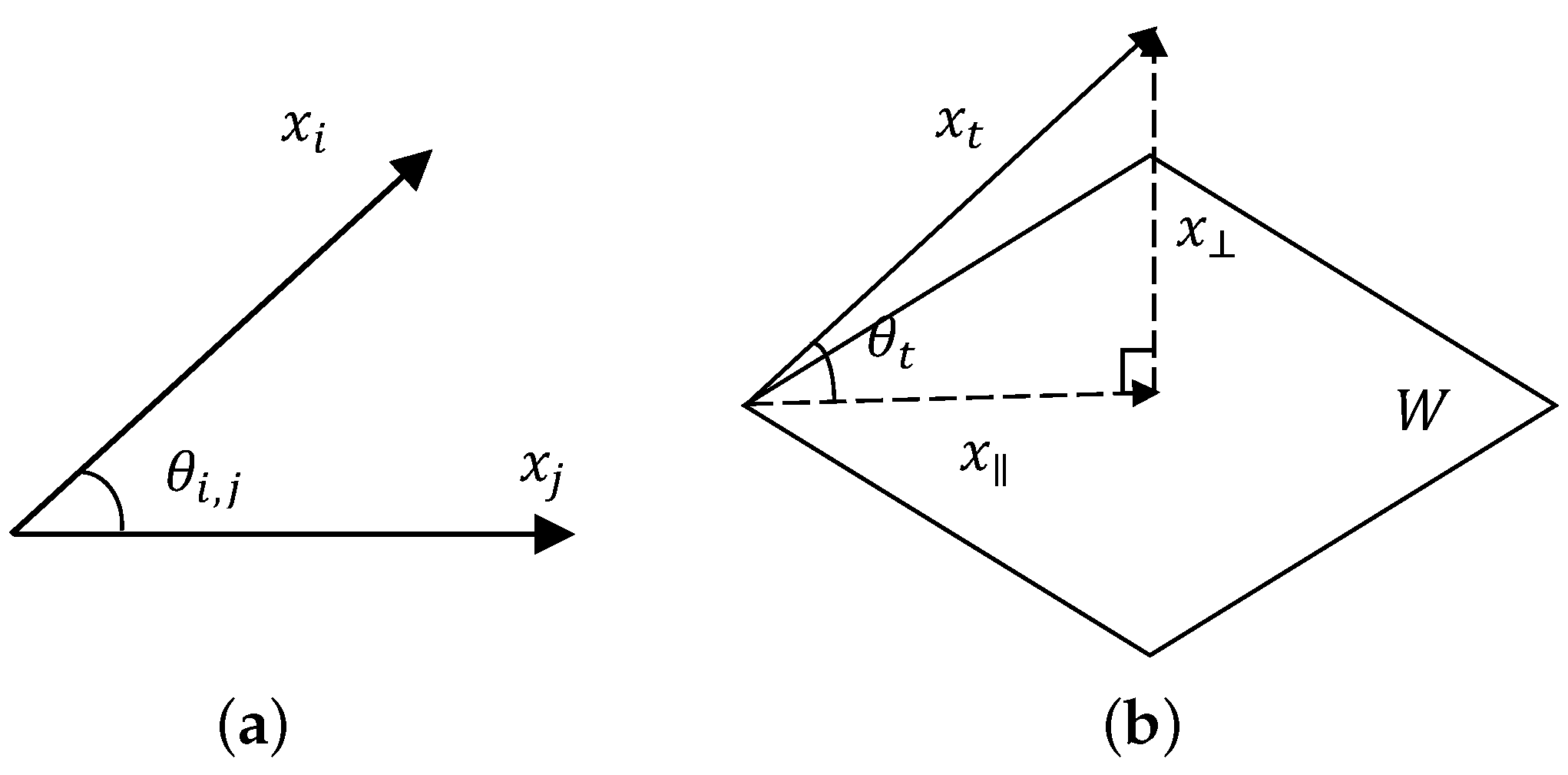
where $x_i^T{x}_j$ denotes the vector inner product; $\parallel x_i\parallel$ denotes the Euclidean norm of $x_i$; and ${\theta }_{i,j}$ denotes the angle between the bands $x_i$ and $x_j$ (for the correlation coefficient, ${\theta }_{i,j}$ lies in the interval $[0,\pi ]$ radians). In Figure 1a, it is evident that the correlation coefficient actually measures the band correlation by computing the angle between two bands. Enlightened by this, we can extend the correlation coefficient to a high-dimensional space, and use the angle between a single band and the hyperplane spanned by other bands to evaluate the correlation among them. Hence, we defined the sine of the angle between a single band and the hyperplane spanned by a set of bands as JCC. Interestingly, when only one band has been selected, the cosine version of JCC is exactly the correlation coefficient between the candidate band and the selected band, therefore, the cosine version of JCC can be regarded as the extension of the correlation coefficient in the high-dimensional space. However, it should be noted that the correlation coefficient is a pairwise correlation metric, namely, it is used to estimate the correlation between two bands, whereas the new metric JCC is able to measure the joint correlation between a single band and multiple bands. Thus, for the BPI model, the band correlation is evaluated jointly instead of pairwise.

Figure 1b shows an example in 3-D, in which $x_t$ and W denote a candidate band and the hyperplane spanned by two selected bands, respectively, and ${\theta }_t$ denotes the angle between them. It should be noted that, for the BPI model, we define that ${\theta }_t$ lies in the interval $[0,\pi /2]$ radians. Then, similar to the correlation coefficient, the larger the value for ${\theta }_t$ is, the less band correlation is. For instance, in the worst case, the ${\theta }_t$ equals zero, the band $x_t$ can be linearly expressed by the selected bands, which means $x_t$ is totally linearly correlated with the selected bands and thus can be regarded as a totally redundant band. In the best case, the ${\theta }_t$ equals ninety degrees, then the band $x_t$ is perpendicular to any band in the selected band set, and it is reasonable to consider that $x_t$ has no correlation with the selected bands. Therefore, the angle between the candidate band and the selected band set can estimate the joint correlation between them.

The JCC or the angle ${\theta }_t$ can be obtained by computing the orthogonal projection of $x_t$ onto the vector space (or hyperplane) W. A vector space is defined as a set that is closed under finite vector addition and scalar multiplication. For instance, suppose that we have obtained k selected bands and the currently selected band set is denoted as $Z=[x_{id\left(1\right)},x_{id\left(2\right)},\dots ,x_{id\left(k\right)}]\in {\mathbb{R}}^{N\times k}$, where $id\left(i\right)$ denotes the index number of the ith selected band, and then the vector space spanned by the bands in Z can be expressed as follows:

$$W=span\left\{Z\right\}=\{x:x=\sum _{i=1}^k{a}_i{x}_{id\left(i\right)},a_i\in \mathbb{R}\}$$

(6)

Then, according to Figure 1b, JCC can be obtained by computing

$$JC{C}_t=sin{\theta }_t=\frac{\parallel x_{\perp }\parallel }{\parallel x_t\parallel }$$

(7)

where $JC{C}_t$ estimates the joint correlation between $x_t$ and Z; and $x_{\parallel }$ is the orthogonal projection of $x_t$ onto W. Similarly, $x_{\perp }$ is the orthogonal projection of $x_t$ onto the orthogonal complement of W. The two orthogonal components can be computed by

$$x_{\parallel }=P{x}_t$$

(8)

$$P=Z{\left(Z^{T}Z\right)}^{-1}{Z}^T$$

(9)

$$x_{\perp }=P^{\perp }{x}_t$$

(10)

$$P^{\perp }=I-P$$

(11)

where I is an identity matrix; P is called the orthogonal projector; and $P^{\perp }$ is the orthogonal complement of P [38]. It is worth noting that P (or $P^{\perp }$) is symmetric and idempotent, i.e.,

$$P=P^T$$

(12)

$$P^2=P$$

(13)

For simplicity, we use the standardized bands (i.e., the unit vector in the direction of each band) to compute the angle between the candidate band and the selected band set. Assume that the standardized bands are denoted as $\overline{X}=[{\overline{x}}_1,{\overline{x}}_2,\dots ,{\overline{x}}_L]\in {\mathbb{R}}^{N\times L}$, and the currently selected band set is denoted as $Z=[{\overline{x}}_{id\left(1\right)},{\overline{x}}_{id\left(2\right)},\dots ,{\overline{x}}_{id\left(k\right)}]\in {\mathbb{R}}^{N\times k}$, then Equation (7) can be simplified as follows:

$$JC{C}_t=\frac{\parallel x_{\perp }\parallel }{\parallel x_t\parallel }=\parallel P^{\perp }{\overline{x}}_t\parallel$$

(14)

Hence, we can use the JCC as the correlation metric $c_t$ for the BPI model, i.e.,

$$c_t=JC{C}_t=\parallel P^{\perp }{\overline{x}}_t\parallel$$

(15)

It should be noted that, although we choose the JCC as the default correlation metric for the BPI model in this paper, other trigonometric functions of ${\theta }_t$ (e.g., $tan{\theta }_t$) or even the angle ${\theta }_t$ itself can also be used as the correlation metric in BPI. However, for $cos{\theta }_t$, it cannot be directly used, because $cos{\theta }_t$ is very close to 1 when there have been several bands obtained; in this case, using its inverse as the correlation metric will cause that BPI is insensitive to the band correlation, too. Therefore, we do not recommend directly using $cos{\theta }_t$ as the correlation metric without additionally proper processing. As for $tan{\theta }_t$ and ${\theta }_t$, when they are, respectively, applied as the correlation metric, the results are almost the same as using $sin{\theta }_t$, which occurs because, when ${\theta }_t$ is close to zero, these three metrics are close to each other. Since JCC (i.e., $sin{\theta }_t$) is more easily computed, we choose it as the default choice for correlation metric.

3.2.2. Incremental Calculation of JCC

However, directly computing JCC is impractical, because the projector P (or $P^{\perp }$) is an $N\times N$ matrix, where N is the number of pixels and is usually very large, which means the calculation and storage of P (or $P^{\perp }$) are unacceptable in practice. Fortunately, JCC can be incrementally calculated by using recursive formulas without computing and storing the projector P or $P^{\perp }$. As aforementioned, JCC is computed by

$$y_t=P^{\perp }{\overline{x}}_t$$

(16)

$$JC{C}_t=sin{\theta }_t=\parallel y_t\parallel$$

(17)

where $y_t$ denotes the orthogonal projection of $x_t$ onto the orthogonal complement of the vector space W, namely, $y_t=x_{\perp }$ (Figure 1b). Assume that the number of desired bands is n; to find all the desired bands, we need perform n rounds of lookups. For the convenience of illustration, in the ith round, $P^{\perp }$ is denoted as $P_i^{\perp }$, and $y_t$ and $sin{\theta }_t$ of the candidate band $x_t$ are, respectively, denoted as follows:

$$y_t^{\left(i\right)}=P_i^{\perp }{\overline{x}}_t$$

(18)

$$JC{C}_t^{\left(i\right)}=sin{\theta }_t^{\left(i\right)}=\parallel y_t^{\left(i\right)}\parallel$$

(19)

After the newly selected band $x_{id\left(i\right)}$ has been found and its normalized band ${\overline{x}}_{id\left(i\right)}$ has been added into Z, the next round of lookup begins. Then, in the $(i+1)$th round, for the same candidate band $x_t$, according to Equations (9)–(13), we have:

$$\begin{array}{cc}\hfill y_t^{\left(i\right)}& =P_i^{\perp }{\overline{x}}_t\hfill \\ & ={\overline{x}}_t-\left[\begin{array}{cc}Z& {\overline{x}}_{id\left(i\right)}\end{array}\right]{\left[\begin{array}{cc}{Z}^{T}Z& Z^T{\overline{x}}_{id\left(i\right)}\\ {\overline{x}}_{id\left(i\right)}^{T}Z& {\overline{x}}_{id\left(i\right)}^T{\overline{x}}_{id\left(i\right)}\end{array}\right]}^{-1}\left[\begin{array}{c}{Z}^T\\ {\overline{x}}_{id\left(i\right)}^T\end{array}\right]{\overline{x}}_t\hfill \\ & =P_i^{\perp }{\overline{x}}_t-P_i^{\perp }{\overline{x}}_{id\left(i\right)}{\left({\overline{x}}_{id\left(i\right)}^T{P}_i^{\perp }{\overline{x}}_{id\left(i\right)}\right)}^{-1}{\overline{x}}_{id\left(i\right)}^T{P}_i^{\perp }{\overline{x}}_t\hfill \\ & =P_i^{\perp }{\overline{x}}_t-P_i^{\perp }{\overline{x}}_{id\left(i\right)}{\left({\overline{x}}_{id\left(i\right)}^T{P}_i^{\perp }{\overline{x}}_{id\left(i\right)}\right)}^{-1}{\overline{x}}_{id\left(i\right)}^T{P}_i^{\perp }{P}_i^{\perp }{\overline{x}}_t\hfill \\ & =y_t^{\left(i\right)}-y_{id\left(i\right)}^{\left(i\right)}(\parallel y_{id\left(i\right)}^{\left(i\right)}{{\parallel }^2)}^{-1}{y_{id\left(i\right)}^{\left(i\right)}}^T{y}_t^{\left(i\right)}\hfill \end{array}$$

(20)

which demonstrates that the current $y_t^{(i+1)}$ is only associated with $y_t^{\left(i\right)}$ and $y_{id\left(i\right)}^{\left(i\right)}$, and both the terms have been computed and stored in the previous round. Moreover, we notice that both $y_t^{\left(i\right)}$ and $y_{id\left(i\right)}^{\left(i\right)}$ are the $N\times 1$ vectors, and $\parallel y_{id\left(i\right)}^{\left(i\right)}{\parallel }^2$ is a scalar, thus, the calculation of Equation (20) only involves low-complexity vector multiplication and scalar multiplication. Furthermore, Equation (20) can be further justified as

$$y_t^{(i+1)}=y_t^{\left(i\right)}-y_{id\left(i\right)}^{\left(i\right)}[{y_{id\left(i\right)}^{\left(i\right)}}^T{y}_t^{\left(i\right)}/\parallel y_{id\left(i\right)}^{\left(i\right)}{\parallel }^2]$$

(21)

where ${\left(y_{id\left(i\right)}^{\left(i\right)}\right)}^T{y}_t^{\left(i\right)}$ is computed first and is also a scalar, thus Equation (21) avoids the generation of the high-order matrix variables during the calculation, which is useful for saving computing time and storage space. By using Equation (21), it is unnecessary to compute P (or $P^{\perp }$) in each round, we can directly obtain the value of JCC (i.e., $sin\theta$) incrementally, and, at the same time, the computational complexity is reduced significantly.

3.3. Information Metric

On the other hand, for the BPI model, we need to choose an effective information metric to evaluate the amounts of information of bands. In this paper, we, respectively, apply two widely-used information metrics, namely, the variance and the information entropy, as the information metric ${\delta }_t$ for the BPI model; and the corresponding methods are denoted as BPI-VAR and BPI-EN, respectively.

The variance is the expectation of the squared deviation of a random variable from its mean; it measures how far a set of (random) numbers are spread out from their average value. In hyperspectral remote sensing, variance is often used to estimate the amounts of information of bands, and the value for variance can be regarded as the classification separability to some extent. For a candidate band $x_t$, its variance is defined as follows:

$$var\left(x_t\right)=\sum _{i=1}^N{(x_{t,i}-{\mu }_t)}^2$$

(22)

where $x_{t,i}$ and ${\mu }_t$ represent the ith pixel and the average of $x_t$, respectively. Then, for the BPI-VAR method, $c_t=sin{\theta }_t$ and ${\delta }_t=var\left(x_t\right)$.

In the field of information theory, the information entropy is defined as the average amount of information produced by a stochastic source of data [39]. It estimates the disorder or uncertainty of a set of variables, and the band that has large entropy can be considered as the band with a large amount of information. Similarly, for the band $x_t$, its entropy is computed by

$$e\left(x_t\right)=-\sum _{i=1}^N{p}_{i}log{p}_i$$

(23)

where $p=[p_1,p_2,\dots ,p_N]$ is the image histogram of the band $x_t$ and is normalized as a probability distribution. Hence, for the BPI-EN method, we have $c_t=sin{\theta }_t$ and ${\delta }_t=e\left(x_t\right)$.

3.4. Number of Selected Bands

In practice, another important issue for BS should be considered is the determination of the number of bands to be selected. Interestingly, the BPI model has the potential to find how many bands should be selected. We find that the score of the newly selected band is always smaller than the previously selected bands’ scores. Based on this property, the BPI-based methods can determine the number of selected bands. According to Equation (4), the scores of two sequentially selected bands $x_{id\left(i\right)}$ and $x_{id(i+1)}$ are measured by:

$$\left\{\begin{array}{c}{s}_{id\left(i\right)}^{\left(i\right)}=c_{id\left(i\right)}^{\left(i\right)}\times {\delta }_{id\left(i\right)}\hfill \\ s_{id(i+1)}^{(i+1)}=c_{id(i+1)}^{(i+1)}\times {\delta }_{id(i+1)}\hfill \end{array}\right.$$

(24)

where $s_{id\left(i\right)}^{\left(i\right)}$ denotes the score of the ith selected band $x_{id\left(i\right)}$. Then, we need to prove that

$$s_{id\left(i\right)}^{\left(i\right)}\ge s_{id(i+1)}^{(i+1)}$$

(25)

However, they have no direct relationship, so we introduce a third variable: $s_{id(i+1)}^{\left(i\right)}$, which is the score of band $x_{id(i+1)}$ in the ith round. Then, it is equivalent to proving that

$$s_{id\left(i\right)}^{\left(i\right)}\ge s_{id(i+1)}^{\left(i\right)}\ge s_{id(i+1)}^{(i+1)}$$

(26)

Obviously, $s_{id\left(i\right)}^{\left(i\right)}$ is larger than $s_{id(i+1)}^{\left(i\right)}$ because the band $x_{id\left(i\right)}$ is the optimal band in the ith round. Hence, we just need to prove that $s_{id(i+1)}^{\left(i\right)}$ is larger than $s_{id(i+1)}^{(i+1)}$, which is equivalent to proving that

$$s_t^{\left(i\right)}\ge s_t^{(i+1)}$$

(27)

Hence, our goal is to prove that for the same candidate band $x_t$, its score of the current round is smaller than that of the previous round. According to Equation (4), it is also equivalent to proving that $c_t^{\left(i\right)}\ge c_t^{(i+1)}$; since JCC is used as the correlation metric in this paper, our final goal is to prove

$$sin{\theta }_t^{\left(i\right)}\ge sin{\theta }_t^{(i+1)},({\theta }_t\in [0,\pi /2])$$

(28)

Hence, we compute the equation as follows:

$$\Delta ={sin}^2{\theta }_t^{\left(i\right)}-{sin}^2{\theta }_t^{(i+1)}={y_t^{\left(i\right)}}^T{y}_t^{\left(i\right)}-{y_t^{(i+1)}}^T{y}_t^{(i+1)}$$

(29)

According to Equation (21), it can be found that

$$\Delta =\frac{\parallel {y_{id\left(i\right)}^{\left(i\right)}}^T{y}_t^{\left(i\right)}{\parallel }^2}{\parallel y_{id\left(i\right)}^{\left(i\right)}{\parallel }^2}\ge 0$$

(30)

Therefore, Equations (25)–(28) have been proven, and we can see that the scores of the newly selected bands decrease as the number of iteration increases. This phenomenon is because, as more bands have been included in the selected band set, the remaining bands are more correlated with the selected band set.

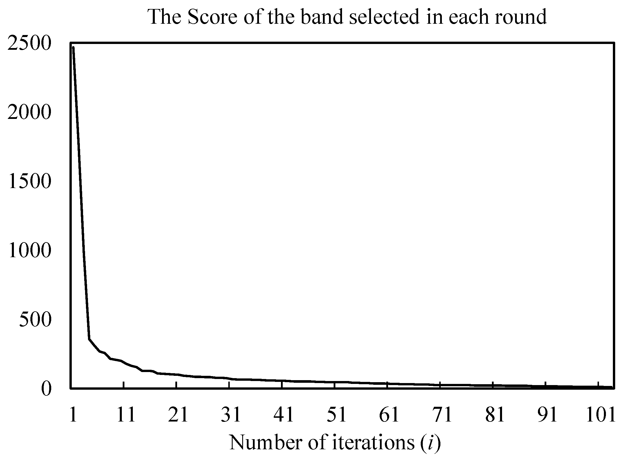
When the number of the selected bands exceeds a specific size, the score of the newly selected band becomes relatively small, which means the contribution of the bands becomes less and adding more bands into the selected band set no longer increases the total amount of information of the band combination significantly, in this case, the BS algorithm can be terminated. For instance, Figure 2 shows the scores of the bands selected by BPI-VAR in each round from a real hyperspectral dataset. It can be seen that the scores of each newly selected band is smaller than that of previously selected band, and the slope of the curve becomes quite small when sufficiently number of bands have been selected, which can be used to determine the number of selected bands. Here, a simple way to compute the decreasing rate is

$$r\left(k\right)=\frac{s_{id\left(k\right)}-s_{id(k-1)}}{s_{id(k-1)}}$$

(31)

where $r\left(k\right)$ denotes the decreasing rate of the kth selected band. Then, during the process of BS, when the average of three sequentially selected bands’ rate is less than a threshold $ϵ$, the BS algorithm can be terminated. In this paper, the parameter $ϵ$ is set to be 0.05 in default.

3.5. Computational Complexity Analysis

The BPI model also has the advantage of high computational efficiency. The correlation metric JCC can be incrementally calculated by using the recursive Equation (21), thus the computation of this part is not computationally complex. As for the computation of amounts of information, its computational complexity depends on the choice of information metrics, and, for most information metrics, the calculation is also not complex. Here, we use the floating point operations (flops) to measure the computational complexity of proposed methods, and the procedures of BPI-based methods are given in Algorithm 1, which shows that the calculation of the JCC has been reduced significantly and only results in about $3nNL$ flops in total; when using the variance as the information metric, the calculation of amounts of information results in about $NL$ flops; and, when using entropy as the information metric, it results in about $2NL$ flops. Therefore, the total flops of BPI-VAR and BPI-EN are about $3nNL+NL$ and $3nNL+2NL$, respectively. This demonstrates that the BPI-based methods have quite good computational efficiencies.

Algorithm 1 The BPI Algorithm

Input: Observations $X=[x_1,x_2,\cdots ,x_L]\in {\mathbb{R}}^{N\times L}$, the number of selected bands n. Here, $id\left(i\right)(i=1,2,\dots ,n)$ denotes the index number of the ith selected band. Band Selection Step 1: Compute the amounts of information of bands in X and denote them as $D=[{\delta }_1,{\delta }_2,\dots ,{\delta }_L]\in {\mathbb{R}}^L$. Step 2: Select the band with maximum information as the initial selected band, which is denoted as $x_{id\left(1\right)}$. Set the initial selected band set as $\mathsf{\Phi }=\left\{x_{id\left(1\right)}\right\}$ Step 3: Let $Y=[y_1,y_2,\cdots ,y_L]=\overline{X}$, where $\overline{X}$ denotes the normalized band set of X, then set counter $i=2$. while $i<n+1$ or (31) is not met do Step 4: Calculate the $c_t$ of the tth normalized band ${\overline{x}}_t,(t=1,2,\dots ,L)$, i.e., $$y_t=y_t-y_{id(i-1)}[y_{id(i-1)}^T{y}_t/\parallel y_{id(i-1)}{\parallel }^2]$$ $$c_t=\parallel y_t\parallel$$ Step 5: Find the band that has the largest score as the optimal band, and add it into $\mathsf{\Phi }$, i.e., $$s_t=c_t\times {\delta }_t$$ $$id\left(i\right)=\underset{t}{argmax}\left(s_t\right)$$ $$\mathsf{\Phi }=\mathsf{\Phi }\cup \left\{x_{id\left(i\right)}\right\}$$ If the tth band $x_t$ has already been selected, its $y_t$ and $s_t$ will not be calculated and compared. Step 6: $i\leftarrow i+1$ end while Output: Selected band set $\mathsf{\Phi }$.

4. Experiments

In this section, we evaluate the performance of the BPI model on three different real-world hyperspectral datasets. Two of implementations of BPI, namely, the BPI-VAR and BPI-EN methods, are used in our experiments. For comparison, six different unsupervised BS methods are used: LCMV Band Correlation Constraint (LCMV-BCC) [10], LCMV Band Correlation Minimization (LCMV-BCM) [10],Volume-Gradient-based BS (VGBS) [21],Exemplar Component Analysis (ECA) [28], Manifold Ranking (MR) [20] and the Simplified OIF-based method (SOIF) [14]. Among these methods, LCMV-BCC and LCMV-BCM are classical BS methods, VGBS; ECA and MR are newly proposed state-of-the-art methods; and SOIF method has a similar design idea with the proposed method. The LCMV-based methods aim to select the bands that best represent the whole image cube, and the representative ability of a candidate band is measured by its correlation with the whole image dataset. VGBS is a geometry-based method, which tries to find the band set with the maximum ellipsoid volume. The bands with the maximum volume gradients are removed one by one, until the desired number of bands remains. ECA is based on an effective clustering algorithm [29], so it performs quite well in practice. MR is based on many advanced machine learning algorithms including clustering, clone selection and manifold ranking [20]. As for SOIF, it is similar to the BPI model and also computes the indexes of bands, the bands with the largest scores are selected as the desired bands. The comparison includes three aspects: pixel classification results, band correlation and computing time. Additionally, some tests about the recommended number of selected bands are also introduced in this section.

4.1. Hyperspectral Datasets

(1)

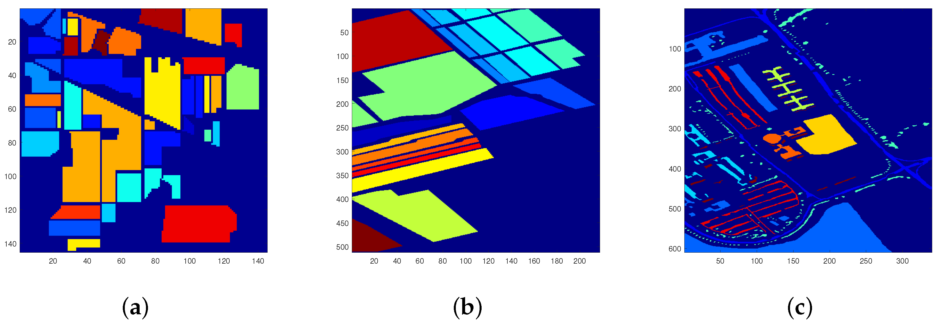
Indian Pine Dataset [40]: The first hyperspectral image we used has been researched extensively. The image was collected by the AVIRIS sensor over the Indian Pine region in Northwestern Indiana in 1992, and it has $145\times 145$ pixels (about 20 m per pixel) and 220 bands with a wavelength range from 400 to 2500 nm (Figure 3a). In our experiments, bands 1–3, 103–112, 148–165, and 217–220 were removed due to atmospheric water vapor absorption and low signal to noise ratio (SNR) [16], leaving 185 valid bands to be used. Of the 16 classes in the image, only nine classes are used in our experiment and the others are removed because of the lack of sufficient samples (

Table 1. Number of samples for ground objects in Indian Pine dataset.

Class	Training Samples	Testing Samples
1. Corn-notill	143	1291
2. Corn-mintill	83	751
3. Grass/Pasture	49	448
4. Grass/Trees	74	673
5. Hay-windrowed	48	441
6. Soybeans-notill	96	872
7. Soybeans-meantill	246	2222
8. Soybeans-clean	61	553
9. Woods	129	1165
Total	929	8416

) [16].

(2)

Salinas Dataset [41]: The second image was collected by the 224-band AVIRIS sensor over Salinas Valley, California, and was characterized by a high spatial resolution (3.7-m pixels) (Figure 3b). The dataset has a medium size of $512\times 217$ pixels, and the spectral range is from 370 to 2507 nm. For this dataset, we discarded the 20 water absorption bands, which were the bands: 108–112, 154–167, and 224. In our experiments, all 16 classes in the Salinas dataset are used.

(3)

Pavia University Dataset [42]: The third image is a hyperspectral image at the University of Pavia acquired by the ROSIS-3 optical sensor (Figure 3c). The dataset has 103 spectral bands with a spectral range from 0.43 to 0.86 $\mathsf{\mu }$m. The image size is $610\times 340$ with a spatial resolution of about 1.3 m. In the image, nine classes are labeled and used: Asphalt, Meadows, Gravel, Trees, Painted Metal Sheets, Bare Soil, Bitumen, Self-Blocking Bricks, and Shadows [43].

4.2. Classification Performance

To evaluate the performance of different methods, the pixel classifications of the three hyperspectral images are conducted, respectively, with two different classifiers: K-Nearest Neighborhood (KNN) and Support Vector Machine (SVM) [44]. In our experiments, the neighbors in KNN are set to be 3; as for SVM, Gaussian Radial Basis Function (RBF) is used as the kernel function and the one-against-all scheme [45] is used for multi-class classification. For all three datasets, we randomly select 10% samples from each class to construct the training set, and the rest are used for testing. In the following, we will discuss the BS results on different images with respect to two classifiers. Two kinds of results are shown in this section: the first kind are the band number-accuracy curves and the second kind are the averaged accuracy bars (i.e., the average of accuracy curve). It should be noted that the classification accuracy is defined as the proportion of correctly classified pixels to all the corresponding class pixels in the image.

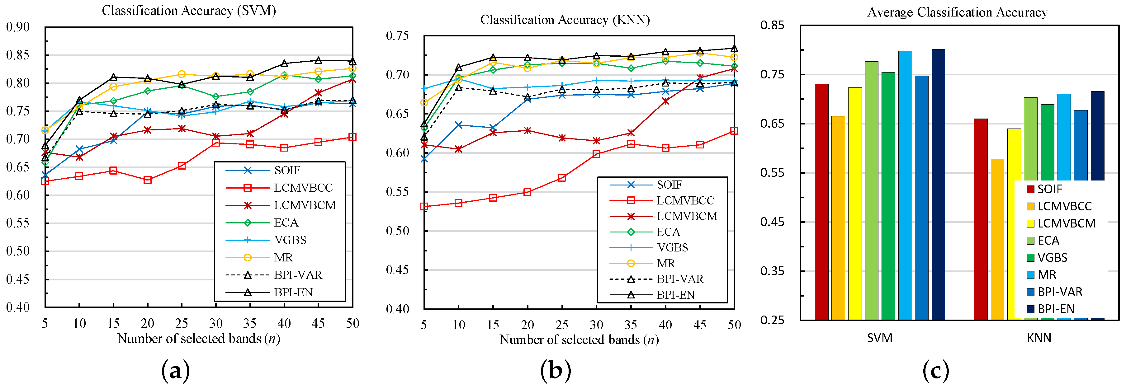
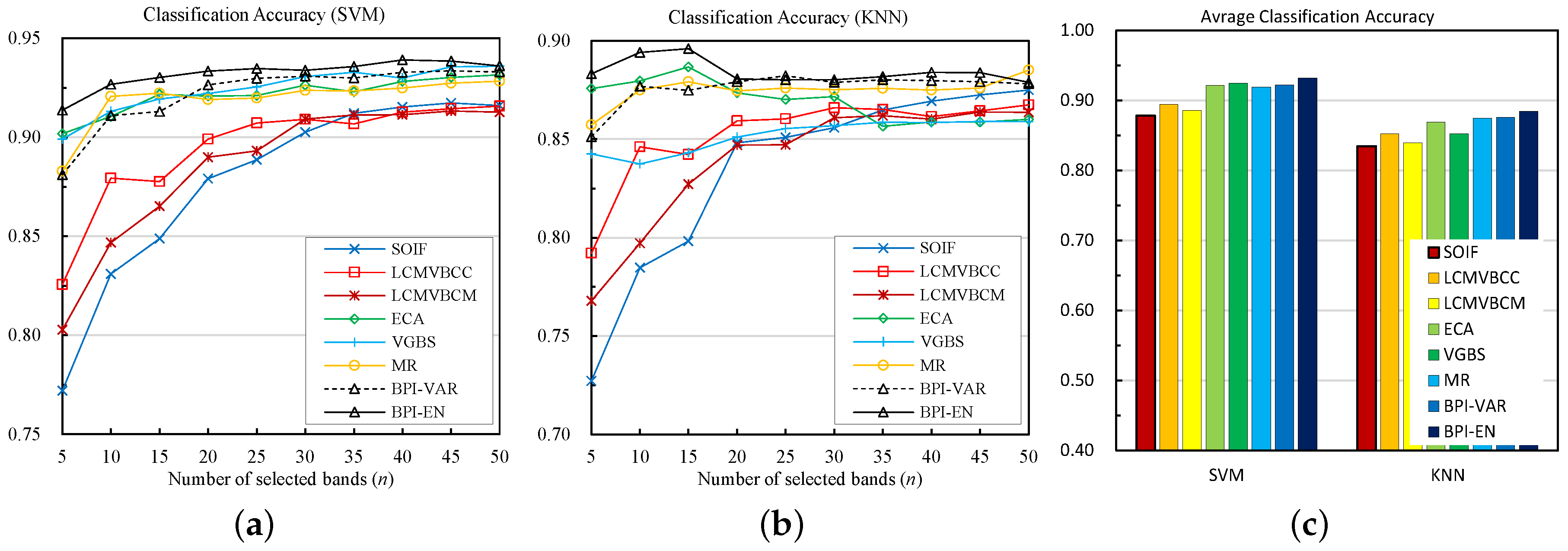
For the Indian Pine dataset, we can see in Figure 4 that the overall classification accuracies of all the methods increase as the number of the selected bands increases. When using SVM, the BPI-EN method shows the best overall performance, followed by MR, ECA, VGBS and BPI-VAR. The performances of VGBS and BPI-VAR are similar to each other. The SOIF, LCMV-BCM and LCMV-BCC methods cannot compete with the two proposed methods, especially when selecting a small number of bands. As for KNN classifier, likewise, BPI-EN performs the best, followed by MR, ECA, VGBS and BPI-VAR. For this classifier, VGBS is slightly superior to BPI-VAR. Additionally, the average results of selecting different numbers of bands are shown in Figure 4c, from which we can see that BPI-EN obtains the best overall classification performance, followed by MR, ECA, VGBS, BPI-VAR, SOIF and LCMV-BCM, whereas the LCMV-BCC method performs poorly.

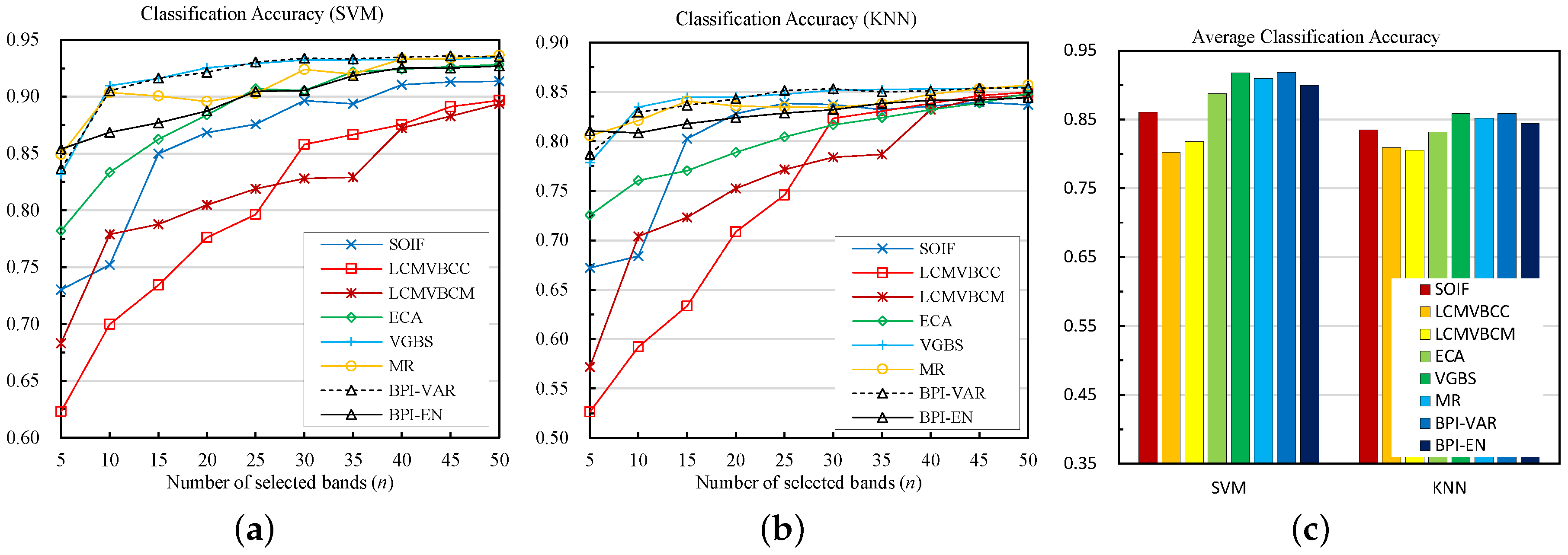
For the Salinas dataset, similarly, BPI-EN outperforms other methods. BPI-VAR, ECA, VGBS and MR also perform well (Figure 5). Other methods cannot compete with these four methods, especially when selecting small numbers of bands. When using SVM, BPI-EN is always superior to others, and BPI-VAR, ECA, VGBS and MR show similar performances, while the remaining methods perform not as well as these four methods. Figure 5c further demonstrates that BPI-EN has the best overall performance, and the overall performance of BPI-VAR is almost the same with ECA and slightly better than those of VGBS and MR. When using KNN, the BPI-EN method still performs the best, followed by BPI-VAR, MR, ECA, VGBS and others. BPI-EN always performs better than others, and BPI-VAR also performs much better the competitors when selecting more than 15 bands. Figure 5c also indicates that the BPI-EN and BPI-VAR methods have the best overall performances for this classifier.

As for the Pavia University dataset, things are a little different (Figure 6). BPI-VAR and VGBS perform the best, followed by MR, BPI-EN, ECA and other methods. When using the SVM classifier, the BPI-VAR and VGBS methods obtain almost the same classification performances, MR also performs well, and the accuracy of ECA is slightly lower than that of MR and BPI-EN. The remaining methods still cannot compete with these best methods. When using KNN, VGBS and BPI-VAR performs best, followed by MR, BPI-EN and other methods. ECA performs worse when compared with the results of SVM, while the BPI-VAR and BPI-EN still obtain good performances. Figure 6c shows the average results of these methods; for this dataset, BPI-VAR and VGBS ranks the first, followed by MR and BPI-EN. These four methods outperform the other methods significantly.

After introducing the classification results, we give some in-depth analysis. In general, the proposed methods are more effective than the other competitors. BPI-EN obtains the best overall performances among all the methods we used. BPI-VAR also performs well; it performs the best on the Pavia University dataset. This is mainly due to the BPI model can evaluate the contribution of bands properly, the band correlation and amounts of information are well considered by the proposed methods. For instance, when compared with the similar method, namely, the SOIF method, our proposed methods have achieved significant improvements on the performances for classification. Even compared with state-of-the-art methods such as MR, ECA and VGBS, the BPI-EN method performs better than them, and the BPI-VAR can compete with them, which verifies that the BPI-based methods are effective. We also notice that the classification performances are influenced by the number of selected bands. There is a phenomenon that the performance is better when the band number is larger. Considering that the purpose of BS is to enhance the computational efficiency and reduce the storage burden at the same time, fewer bands while good classification performance is encouraged for a BS method; therefore, if the selected band number is not large but the performance of classification is satisfying, we can think that the BS method is effective and of great value. The proposed methods (especially the BPI-EN method) have shown satisfactory overall performances in experiments, and when selecting a small number of bands, the superiority is more evident, which demonstrates that the BPI-based methods are valuable and have a good significance in practical applications. Additionally, we also conduct experiments using the whole image cube and the results are as follows: Indian Pine [SVM (0.8382) and KNN (0.7449)], Salinas [SVM (0.9406) and KNN (0.8806)] and Pavia University [SVM (0.9396) and KNN (0.8691)]. Comparing the BS methods (Figure 4, Figure 5 and Figure 6) with the full band method, we can find that the proposed BPI-EN method does not reduce the classification accuracy very much. For each image and classifier, abandoning most redundant bands only leads to a small reduction in accuracy (<3%) for the classification task. This denotes that the proposed methods are very effective. Although only a limited number of bands are selected, we can achieve an acceptable performance. Therefore, the classification experiments on three different datasets verify that the bands selected by the proposed method are informative for classification, and the proposed methods are highly accurate BS methods.

4.3. Band Correlation

In this section, we evaluate the average band correlation among the bands selected by different methods. We use the average correlation coefficients (ACC) to estimate the overall band correlation among the selected bands. The larger the value for JCC is, the larger the average band correlation is.

Table 2. Correlation of the fifteen bands selected from different datasets.

ACC	SOIF	LCMVBCC	LCMVBCM	VGBS	ECA	MR	BPI-VAR	BPI-EN
Indian	0.65	0.98	0.99	0.19	0.30	0.25	0.34	0.17
Salinas	0.79	0.88	0.88	0.39	0.46	0.22	0.38	0.32
PaviaU	0.99	0.98	0.99	0.58	0.66	0.67	0.50	0.54

shows the ACC of the fifteen bands selected from different datasets, and the index numbers of the fifteen bands selected from the Indian Pine dataset are listed in

Table 3. Fifteen bands selected by different methods for the Indian Pine dataset.

	Fifteen Bands
SOIF	15	20	21	22	23	24	25	26	27	28	29	30	31	72	88
LCMV-BCC	106	135	139	154	160	165	167	178	179	180	181	182	183	184	185
LCMV-BCM	103	104	106	107	110	117	120	140	143	154	160	165	168	178	179
VGBS	10	15	17	20	26	29	31	32	36	54	58	59	72	85	86
ECA	1	10	28	29	31	32	33	54	58	59	72	87	95	97	156
MR	4	25	39	50	52	55	58	61	131	151	153	159	161	162	185
BPI-VAR	14	15	16	17	19	22	26	29	30	31	32	39	54	58	72
BPI-EN	5	9	22	23	30	37	39	43	54	55	67	73	108	121	142

. In Table 2, the bands obtained by SOIF and the two LCMV-based methods are highly correlated, whereas the selected bands obtained by the other methods are with much lower correlation. Furthermore, according to Table 3, it can be found that most of the bands obtained by the SOIF, LCMV-BCC and LCMV-BCM methods are neighboring bands, whereas the other five methods select less neighboring bands. In fact, for the hyperspectral images, the neighboring bands are usually highly correlated with each other, so the methods that select too many neighboring bands cannot ensure that the selected band set has low correlation, and, thus, may result in relatively poor classification performances. The results in Table 2 and Table 3 and Figure 4, Figure 5 and Figure 6 have verified this point; the bands selected by the proposed methods, MR, ECA and VGBS are with low correlation, and, correspondingly, the classification performances of them are relatively better than others.

It is worth noting that these results also verify that the SOIF method cannot always consider the band correlation properly. It can be seen in Table 2 that, although SOIF can consider the band correlation to some extent, it does not perform consistently. For instance, when selecting bands from the Indian Pine and Salinas datasets, the selected bands are with acceptable correlation, but, when selecting bands from the Pavia University dataset, they are with quite high correlation. This occurs because that the SOIF method uses the correlation coefficients as the denominator of the objective function, and the correlation coefficients between neighboring bands are often very close to 1 because of their high correlation with each other, which means, for most candidate bands, their SOIF’s denominators are almost the same, and thus their scores are mainly determined by the amounts of information of bands. Therefore, the SOIF method sometimes cannot pay sufficiently enough attention on the band correlation, which deteriorates its performance. As for the two LCMV-based methods, they also select one band for each time, and the band that is the most correlated with the whole image cube would be regarded as the optimal band. It is easy to find that LCMV-based methods also do not pay much attention on the band correlation among the selected bands, therefore, the bands obtained by this kind of methods are also usually highly correlated.

4.4. Computing Time

In this section, we compare the computing time of different methods. The computing time of selecting fifteen bands from different datasets is listed in

Table 4. Computing time of selecting fifteen bands from different datasets.

Time (s)	SOIF	LCMVBCC	LCMVBCM	VGBS	ECA	MR	BPI-VAR	BPI-EN
Indian	0.26	2.24	1.88	2.09	1.85	2.67	0.62	0.79
Salinas	2.99	21.62	17.16	24.09	17.32	47.01	3.83	4.14
PaviaU	1.32	13.24	8.84	7.78	6.64	29.54	3.23	3.55

.

In Table 4, the proposed methods have good computational efficiencies. Among all the methods, SOIF spends the least time, followed by BPI-VAR and BPI-EN, of which computing time is just a little more than that of SOIF, but is always lower than the other methods’ computing time. The SOIF method has a small number of steps, so it has a good computational efficiency. Specifically, the SOIF method only needs to compute the standard deviation of each band and the correlation coefficients of all the adjacent band pairs. All these steps only result in about $2NL$ flops, where N and L are the numbers of pixels and bands, respectively. As for the proposed methods, the procedures not only include the calculation of amounts of information but also the computation of JCCs, which results in the additional computational complexity. However, due to the adoption of recursive formulas, JCCs can be computed incrementally, which reduces the complexity of the algorithm significantly. For instance, the total computational complexity of BPI-VAR is about $3nNL+NL$, which is slightly larger than that of SOIF. Considering that the proposed methods have shown much better classification performances than the SOIF method, a little more time cost is acceptable. When compared with the methods excluding SOIF, the BPI-based methods cost the least time. VGBS needs to compute the covariance matrix of total bands and perform Singular Value Decomposition (SVD), which result in about $N{L}^2+L^3$ flops, so its computational complexity is higher than the BPI-based methods. Although the clustering algorithm applied by ECA is quite effective for most clustering algorithms, the computational burden is still high when compared with the proposed methods. The MR is quite complicated; it involves clustering, clone selection and manifold ranking, which are all time-consuming. Although the MR method performs quite well in the classification experiments, it costs the most time, which is a significant drawback of this method. The LCMV-based methods require to evaluate the correlation between each candidate band and the whole image cube, which is relatively computational complex, so they cost much time, too. To sum up, these results have identified that the proposed methods have good computational efficiencies and can obtain the desired bands in a short time.

4.5. Number of Selected Bands

In practice, it is difficult to determine the number of bands to be selected, a reasonable way is to choose the number of bands close to the number of classes in the dataset. Generally, the number of classes can be determined by using a virtual dimensionality (VD) estimation approach proposed in [46], but this results in additional computational burden and the classes number is sometimes not well estimated because it is also difficult to choose suitable values for the parameters in VD. Therefore, if the BS method can determine the number of bands properly and not increase the computational complexity very much, we can think the method is of great value. Interestingly, the proposed BPI-based methods have the potential to determine the number of selected bands automatically, and, most importantly, the parameters in our strategy of determining the selected bands number can be set easily and this process causes little additional computational burden in applications, therefore, the BPI model has a good value for practical applications.

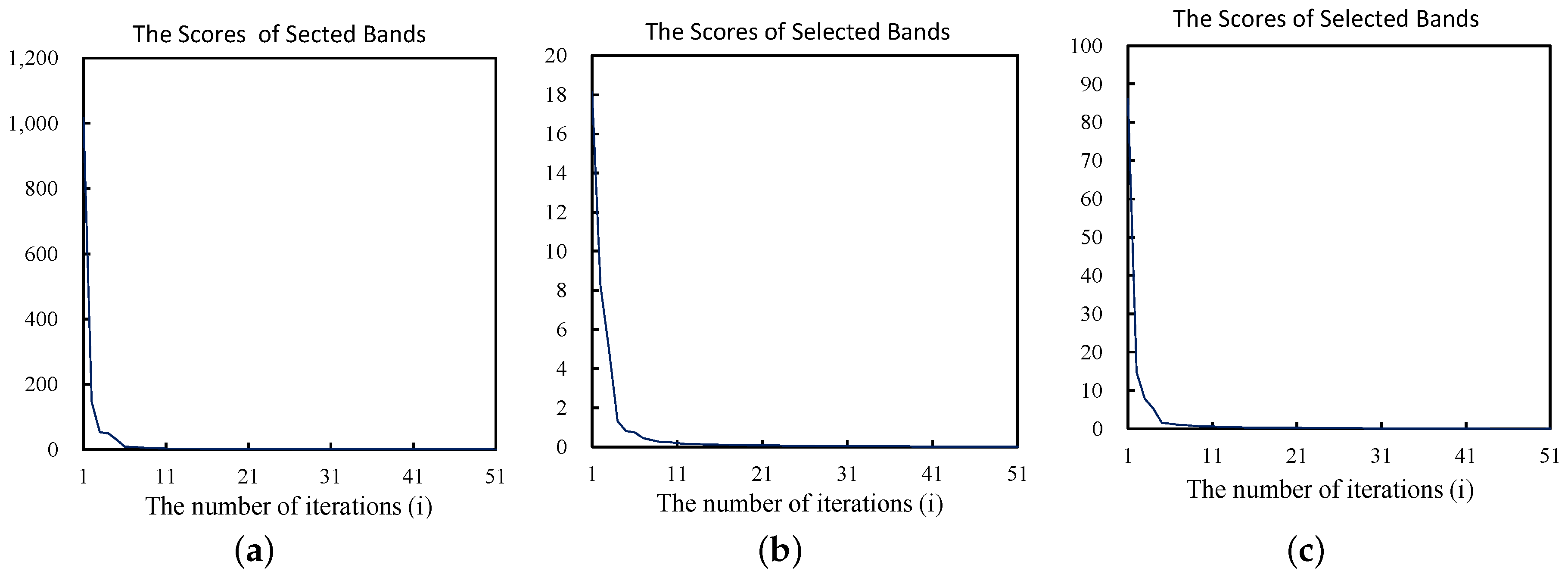
Therefore, in this section, we use the strategy described in Section 3.4 as the stop criterion for the proposed BS algorithm and test the recommended number of selected bands. For all the three datasets, we set the parameters $ϵ$ as 0.05, and the recommended numbers (n) of selected bands are, respectively, listed in

Table 5. Recommended Number of Selected Bands ($ϵ=0.05$).

	Indian Pine	Salinas	Pavia U
BPI-EN	12	24	16
BPI-VAR	7	15	20

, from which we can see that the recommended numbers are suitable. Furthermore, taking the BPI-VAR method as an example, the scores of the bands selected from different datasets in each iteration are illustrated in Figure 7, from which we can see that the curves of scores have clear inflection points and the slope of curve becomes quite small when sufficient number of bands have been selected. When the number exceeds the recommended number, the scores of the newly selected bands are relatively small and can be neglected when compared with the first several selected bands’ scores. Considering that the scores of bands also denote the contribution of bands, it is reasonable to consider that the remaining bands cannot supply much additional information for the current band combination, and, thus, the BS algorithm can be stopped.

4.6. Summary

From all the experiments on three different hyperspectral datasets, some important results can be summarized. In band selection, both the amount of information and band correlation should be considered. The BPI model can find a good trade-off between the amount of information and band correlation, and the experimental results have verified that the bands obtained by the proposed methods are informative and distinctive, and therefore the selected bands can achieve a satisfactory performance. In our experiments, the performance of BPI-EN is better than other methods, even when compared with the state-of-the-art methods such as MR, VGBS and ECA. The BPI-VAR also shows satisfactory performances in applications, its performance is close to that of the VGBS method and much better than other competitive methods excluded MR and ECA. It is worth noting that BPI-EN performs slightly better than BPI-VAR, which demonstrates that the choice of information metric has significant influence on the performance of the BPI method. Additionally, the proposed methods always produce good and stable performances of classification in any datasets, which demonstrates that the proposed methods have a good robustness. Furthermore, the BPI model has a good computational efficiency, and the experimental results verifies that the BPI-based methods can obtain desired bands in a short time. Finally, the BPI model also has the potential to determine the suitable number of bands to be selected; the recommended number can be regarded as a reference value for the number of selected bands. In conclusion, the effectiveness of BPI has been verified.

5. Conclusions

In this paper, a Band Priority Index (BPI) model for hyperspectral feature selection is proposed to effectively find a diverse band combination that contains discriminative and informative bands for hyperspectral image analysis. The BPI model adopts the SFS strategy, so the desired bands are obtained one by one. A new objective function is designed for BPI, and it consists of two parts: the information metric and the correlation metric. To evaluate the correlation between a candidate band and the selected band set, we proposed a new correlation metric named the joint correlation coefficient (JCC), which is defined as the sine of the angle between the candidate band and the hyperplane determined by selected bands. JCC can estimate the band correlation between a single band and multiple bands jointly instead of pairwise. The variance and entropy are, respectively, chosen as the information metric for BPI, and thus, we give two implementations of BPI, i.e., the BPI-VAR and BPI-EN methods. Experimental results on three different datasets demonstrate that the BPI-based methods are highly efficient and accurate BS methods. Moreover, the BPI-based methods have the potential to determine the number of bands to be selected. Finally, our future research interest is to find effective information metrics to improve the BPI model’s performance.

References

- Landgrebe, D. Hyperspectral image data analysis. IEEE Signal Process. Mag. 2002, 19, 17–28. [Google Scholar] [CrossRef]
- Landgrebe, D. On Information Extraction Principles for Hyperspectral Data; Purdue University: West Lafayette, IN, USA, 1997; 34p. [Google Scholar]
- Brown, A.J. Spectral curve fitting for automatic hyperspectral data analysis. IEEE Trans. Geosci. Remote Sens. 2006, 44, 1601–1608. [Google Scholar] [CrossRef] [Green Version]
- Damodaran, B.B.; Courty, N.; Lefèvre, S. Sparse Hilbert Schmidt independence criterion and surrogate-kernel-based feature selection for hyperspectral image classification. IEEE Trans. Geosci. Remote Sens. 2017, 55, 2385–2398. [Google Scholar] [CrossRef]
- Jolliffe, I.T. Principal Component Analysis and Factor Analysis. In Principal Component Analysis; Springer: Berlin, Germany, 1986; pp. 115–128. [Google Scholar]
- Lee, D.D.; Seung, H.S. Learning the parts of objects by non-negative matrix factorization. Nature 1999, 401, 788–791. [Google Scholar] [CrossRef] [PubMed]
- Hyvärinen, A.; Hurri, J.; Hoyer, P.O. Independent component analysis. In Natural Image Statistics; Springer: London, UK, 2009; pp. 151–175. [Google Scholar]
- Roweis, S.T.; Saul, L.K. Nonlinear dimensionality reduction by locally linear embedding. Science 2000, 290, 2323–2326. [Google Scholar] [CrossRef] [PubMed]
- Green, A.A.; Berman, M.; Switzer, P.; Craig, M.D. A transformation for ordering multispectral data in terms of image quality with implications for noise removal. IEEE Trans. Geosci. Remote Sens. 1988, 26, 65–74. [Google Scholar] [CrossRef] [Green Version]
- Chang, C.I.; Wang, S. Constrained band selection for hyperspectral imagery. IEEE Trans. Geosci. Remote Sens. 2006, 44, 1575–1585. [Google Scholar] [CrossRef]
- Chang, C.I.; Du, Q.; Sun, T.L.; Althouse, M.L. A joint band prioritization and band-decorrelation approach to band selection for hyperspectral image classification. IEEE Trans. Geosci. Remote Sens. 1999, 37, 2631–2641. [Google Scholar] [CrossRef]
- Guo, B.; Gunn, S.R.; Damper, R.I.; Nelson, J.D. Band selection for hyperspectral image classification using mutual information. IEEE Geosci. Remote Sens. Lett. 2006, 3, 522–526. [Google Scholar] [CrossRef]
- Chavez, P.; Berlin, G.L.; Sowers, L.B. Statistical method for selecting landsat MSS. J. Appl. Photogr. Eng. 1982, 8, 23–30. [Google Scholar]
- Xijun, L.; Jun, L. An adaptive band selection algorithm for dimension reduction of hyperspectral images. In Proceedings of the International Conference on Image Analysis and Signal Processing (IASP 2009), Taizhou, China, 11–12 April 2009; pp. 114–118. [Google Scholar]
- Sheffield, C. Selecting band combinations from multispectral data. Photogramm. Eng. Remote Sens. 1985, 51, 681–687. [Google Scholar]
- Liu, X.S.; Ge, L.; Wang, B.; Zhang, L.M. An unsupervised band selection algorithm for hyperspectral imagery based on maximal information. J. Infrared Millim. Waves 2012, 31, 166–176. [Google Scholar] [CrossRef]
- Sotoca, J.M.; Pla, F.; Sanchez, J.S. Band selection in multispectral images by minimization of dependent information. IEEE Trans. Syst. Man Cybern. Part C (Appl. Rev.) 2007, 37, 258–267. [Google Scholar] [CrossRef]
- Du, Q.; Yang, H. Similarity-based unsupervised band selection for hyperspectral image analysis. IEEE Geosci. Remote Sens. Lett. 2008, 5, 564–568. [Google Scholar] [CrossRef]
- Zhang, W.; Li, X.; Dou, Y.; Zhao, L. Fast linear-prediction-based band selection method for hyperspectral image analysis. J. Appl. Remote Sens. 2018, 12, 016027. [Google Scholar] [CrossRef]
- Wang, Q.; Lin, J.; Yuan, Y. Salient band selection for hyperspectral image classification via manifold ranking. IEEE Trans. Neural Netw. Learn. Syst. 2016, 27, 1279–1289. [Google Scholar] [CrossRef] [PubMed]
- Geng, X.; Sun, K.; Ji, L.; Zhao, Y. A fast volume-gradient-based band selection method for hyperspectral image. IEEE Trans. Geosci. Remote Sens. 2014, 52, 7111–7119. [Google Scholar] [CrossRef]
- Wang, L.; Jia, X.; Zhang, Y. A novel geometry-based feature-selection technique for hyperspectral imagery. IEEE Geosci. Remote Sens. Lett. 2007, 4, 171–175. [Google Scholar] [CrossRef]
- Zare, A.; Gader, P. Hyperspectral band selection and endmember detection using sparsity promoting priors. IEEE Geosci. Remote Sens. Lett. 2008, 5, 256–260. [Google Scholar] [CrossRef]
- Zhang, W.; Li, X.; Zhao, L. Hyperspectral band selection based on triangular factorization. J. Appl. Remote Sens. 2017, 11, 025007. [Google Scholar] [CrossRef]
- Mitra, P.; Murthy, C.; Pal, S.K. Unsupervised feature selection using feature similarity. IEEE Trans. Pattern Anal. Mach. Intell. 2002, 24, 301–312. [Google Scholar] [CrossRef] [Green Version]
- Qian, Y.; Yao, F.; Jia, S. Band selection for hyperspectral imagery using affinity propagation. IET Comput. Vis. 2009, 3, 213–222. [Google Scholar] [CrossRef]
- Frey, B.J.; Dueck, D. Clustering by passing messages between data points. Science 2007, 315, 972–976. [Google Scholar] [CrossRef] [PubMed]
- Sun, K.; Geng, X.; Ji, L. Exemplar component analysis: A fast band selection method for hyperspectral imagery. IEEE Geosci. Remote Sens. Lett. 2015, 12, 998–1002. [Google Scholar]
- Rodriguez, A.; Laio, A. Clustering by fast search and find of density peaks. Science 2014, 344, 1492–1496. [Google Scholar] [CrossRef] [PubMed]
- Ahmad, M.; Haq, D.I.U.; Mushtaq, Q.; Sohaib, M. A new statistical approach for band clustering and band selection using K-means clustering. IACSIT Int. J. Eng. Technol. 2011, 3, 606–614. [Google Scholar]
- MartÍnez-UsÓMartinez-Uso, A.; Pla, F.; Sotoca, J.M.; García-Sevilla, P. Clustering-based hyperspectral band selection using information measures. IEEE Trans. Geosci. Remote Sens. 2007, 45, 4158–4171. [Google Scholar] [CrossRef]
- Datta, A.; Ghosh, S.; Ghosh, A. Combination of clustering and ranking techniques for unsupervised band selection of hyperspectral images. IEEE J. Sel. Top. Appl. Earth Obs. Remote Sens. 2015, 8, 2814–2823. [Google Scholar] [CrossRef]
- Pudil, P.; Ferri, F.; Novovicova, J.; Kittler, J. Floating search methods for feature selection with nonmonotonic criterion functions. In Proceedings of the 12th IAPR International Conference on Pattern Recognition, 1994, Vol. 2—Conference B: Computer Vision & Image Processing, Jerusalem, Israel, 9–13 October 1994; Volume 2, pp. 279–283. [Google Scholar]
- Zhong, C.; Li, L.; Bu, F. Study of modified band selection methods of hyperspectral image based on optimum index factor. In Proceedings of the International Symposium on Optoelectronic Technology and Application 2014: Optical Remote Sensing Technology and Applications, Beijing, China, 13–15 May 2014; Volume 9299, p. 929911. [Google Scholar]
- Zhang, L.; Shao, Z.F. Hyperspectral remote sensing image classification based on improved OIF and SVM algorithm. Sci. Surv. Mapp. 2014, 9263, 92632P. [Google Scholar]
- Jain, A.; Zongker, D. Feature selection: Evaluation, application, and small sample performance. IEEE Trans. Pattern Anal. Mach. Intell. 1997, 19, 153–158. [Google Scholar] [CrossRef]
- Fukunaga, K. Introduction to Statistical Pattern Recognition; Academic Press: Cambridge, MA, USA, 2013. [Google Scholar]
- Zhang, X.D. Matrix Analysis and Applications; Cambridge University Press: Cambridge, UK, 2017. [Google Scholar]
- Kullback, S. Information Theory and Statistics; Courier Corporation: North Chelmsford, MA, USA, 1997. [Google Scholar]
- Baumgardner, M.F.; Biehl, L.L.; Landgrebe, D.A. 220 Band AVIRIS Hyperspectral Image Data Set: June 12, 1992 Indian Pine Test Site 3. Purdue Univ. Res. Repos. 2015. [Google Scholar] [CrossRef]
- Gualtieri, A.; Chettri, S.R.; Cromp, R.; Johnson, L. Support Vector Machine Classifiers as Applied to AVIRIS Data. In Proceedings of the Summaries of the Eighth JPL Airborne Earth Science Workshop, Pasadena, CA, USA, 9–11 February 1999. [Google Scholar]
- Dópido, I.; Li, J.; Gamba, P.; Plaza, A. A New Hybrid Strategy Combining Semisupervised Classification and Unmixing of Hyperspectral Data. IEEE J. Sel. Top. Appl. Earth Obs. Remote Sens. 2014, 7, 3619–3629. [Google Scholar] [CrossRef]
- Sui, C.; Tian, Y.; Xu, Y.; Xie, Y. Unsupervised band selection by integrating the overall accuracy and redundancy. IEEE Geosci. Remote Sens. Lett. 2015, 12, 185–189. [Google Scholar]
- Duda, R.O.; Hart, P.E.; Stork, D.G. Pattern Classification; Wiley: New York, NY, USA, 1973; Volume 2. [Google Scholar]
- Rifkin, R.; Klautau, A. In defense of one-vs-all classification. J. Mach. Learn. Res. 2004, 5, 101–141. [Google Scholar]
- Chang, C.I.; Du, Q. Estimation of number of spectrally distinct signal sources in hyperspectral imagery. IEEE Trans. Geosci. Remote Sens. 2004, 42, 608–619. [Google Scholar] [CrossRef]
Figure 1.
The geometric explanation of the correlation coefficient and the new correlation metric: (a) the correlation coefficient; and (b) the joint correlation metric (here, for illustration convenience, assume that each band is a 3 by 1 vector).
Figure 2.
The scores of the bands selected by BPI-VAR from Pavia University dataset (Section 4.1).
Figure 3.
Ground truth maps of different datasets: (a) Indian Pine dataset; (b) Salinas dataset; and (c) Pavia University dataset.
Figure 4.
Classification results of the Indian Pine dataset: (a) SVM; (b) KNN; and (c) Average accuracy Bars.
Figure 5.
Classification results of the Salinas dataset: (a) SVMl (b) KNNl and (c) Average accuracy Bars.
Figure 6.
Classification results of the Pavia University dataset: (a) SVM; (b) KNN; and (c) Average accuracy Bars.
Figure 7.
Scores of the selected bands obtained by the BPI-VAR method: (a) Indian Pine dataset; (b) Salinas dataset; and (c) Pavia University dataset.