Vegetation Water Use Based on a Thermal and Optical Remote Sensing Model in the Mediterranean Region of Doñana

Abstract

Terrestrial evapotranspiration (ET) is a central process in the climate system, is a major component in the terrestrial water budget, and is responsible for the distribution of water and energy on land surfaces especially in arid and semiarid areas. In order to inform water management decisions especially in scarce water environments, it is important to assess ET vegetation use by differentiating irrigated socio-economic areas and natural ecosystems. The global remote sensing ET product MOD16 has proven to underestimate ET in semiarid regions where ET is very sensitive to soil moisture. The objective of this research was to test whether a modified version of the remote sensing ET model PT-JPL, proven to perform well in drylands at Eddy Covariance flux sites using the land surface temperature as a proxy to the surface moisture status (PT-JPL-thermal), could be up-scaled at regional levels introducing also a new formulation for net radiation from various MODIS products. We applied three methods to track the spatial and temporal characteristics of ET in the World Heritage UNESCO Doñana region: (i) a locally calibrated hydrological model (WATEN), (ii) the PT-JPL-thermal, and (iii) the global remote sensing ET product MOD16. The PT-JPL-thermal showed strong agreement with the WATEN ET in-situ calibrated estimates (ρ = 0.78, ρ_1month-lag = 0.94) even though the MOD16 product did not (ρ = 0.48). The PT-JPL-thermal approach has proven to be a robust remote sensing model for detecting ET at a regional level in Mediterranean environments and it requires only air temperature and incoming solar radiation from climatic databases apart from freely available satellite products.

1. Introduction

The global water cycle is changing due to the combined effects of climate change and human interventions during the 21st century [1]. One of the greatest challenges is keeping water consumption at sustainable levels, which is more complex due to the increasing population in a context of climate uncertainty [2,3] and 3.5–4.4 billion people estimated under water scarcity conditions in 2050 [4]. Many regions of the world can expect a combination of increasing temperatures (largely increasing evaporative demand) and decreasing precipitation patterns, which leads to increased stress on tackling water demand [5]. A prime example of this is the Mediterranean region, which is consistently projected as a “hotspot” of drying trends and prolonged water scarcity conditions [6,7].

The Iberian Peninsula is predicted to be among the most affected areas by severe droughts by the end of the 21st century [8]. In this region, where irrigated agriculture represents over 80% of the total extracted water [9], land use shifts towards higher market-valued crops represent a major driver of change, which will markedly increase water withdrawals [10]. In the Guadalquivir basin in Spain, irrigation water requirements are expected to increase between 15% and 20% by 2050 [11]. This may cause a redistribution of water between the surface and groundwater [12]. Monitoring the variations in the hydrological cycle components more closely, among them evapotranspiration (ET), is of major importance in countries facing intensified drought spills [13,14].

After precipitation, ET is the major component in the terrestrial water budget [15]. Evapotranspiration at specific locations can be estimated by using methods such as lysimeters, the Bowen-ratio, or Eddy Covariance (EC) [16]. However, ET estimations at large-scales are complex to achieve due to spatial heterogeneity in the land surface [17,18,19]. As the only connecting term between the water cycle and the land surface energy budget [20,21,22], ET can be estimated by hydrological models (HMs) relying on the water balance or by land surface models (LSMs) computed through the mass-transfer equations between the land surface and the atmosphere [23].

Conceptual lumped HMs consider an undivided entity with individual values of input variables and parameters [24]. Spatially distributed HMs or prognostic LSMs enable ET to be estimated at large scales in a spatially explicit manner [25]. This type of models requires a priori information on land use and surface properties, which are not always up-to-date and may be complex for retrieving in situations of fast land use changes such as new irrigation developments. Diagnostic or historical LSMs using remote sensing (RS) datasets to prescribe vegetation and other surface variables can provide spatially distributed fluxes and fast updating on the land surface [26,27]. Diagnostic RS-LSMs need limited a priori data on soil and vegetation parameters to estimate ET and can rely on remotely sensed land surface temperature (LST) as a proxy to the surface moisture status [28].

The complexity of RS-based models to retrieve ET depends on the process considered [29,30]. ET can be directly estimated as a residual of the surface energy balance equation or can be based on potential evapotranspiration adjusted to actual rates using different constraints factors from remote sensing. The Penman-Monteith (PM) equation [31,32] is the base to compute ET in some global RS-ET products such as the first widely available ET product MOD16 [33,34] whose main challenge relies on estimating surface and aerodynamic resistances to the water vapor [35]. Hu et al. [36] found that MOD16 best performs in temperate and fully humid climates and produces a consistent underestimation of ET in semiarid regions such as Spain, Portugal, the neighborhood of the Black Sea and the Caspian Sea, and semiarid climatic zones in the conterminous United States [37]. In these regions and under water stress conditions, ET is very sensitive to soil moisture. In MOD16, canopy resistance to water vapor relies on vegetation-related RS inputs (e.g., LAI) [38] and stomatal conductance while soil resistance to water vapor relies on the vapor pressure deficit (VPD) and relative humidity (RH), which are indicators of water stress [33,34]. The Priestley-Taylor equation [39] bridges the limitation of estimating these resistances by using an empirical multiplier α_PT [40]. The Priestley-Taylor Jet Propulsion Laboratory (PT-JPL) model combines the PT-approach with the reduction of potential ET based on eco-physiological constraints to land-atmosphere water fluxes [41]. With the aim to minimize the need for RH climatic reanalysis data and to improve the performance in semiarid regions, García et al. [42] proposed a modification of the PT-JPL model (PT-JPL-thermal herein) by introducing the LST with a thermal inertia approach as a proxy to the soil moisture status.

This approach has proven to perform well in the drylands under Mediterranean and monsoonal conditions and to perform better than other RS models as the PM model adapted by Leuning et al. [15]. Although the PT-JPL-thermal model has been benchmarked at EC flux sites [42], it has not been tested with modelled net radiation or at regional levels. The main objectives of this work were: (i) to assess whether the RS PT-JPL-thermal model that uses the thermal inertia approach for soil evaporation can perform similarly to a hydrological model calibrated with in-situ data that requires soil moisture-associated parameters to retrieve ET, (ii) to compare and assess the ET derived from the PT-JPL-thermal against the global ET product MOD16, which estimates soil evaporation as a function of VPD and RH climatic reanalysis, in the Mediterranean region of Doñana including natural ecosystems (wetland, shrubland, and coniferous forest) and irrigated areas (mixed-irrigated areas and rice fields).

2. Study Area

The study area presents Mediterranean climate under Atlantic influence with warm and dry summers and temperate and semi-humid winters. The temperatures range from 24 °C on average in the summertime to 10 °C on average in the winter [43]. The average rainfall is about 560 mm of which more than 80% occurs between October and March. The study area covers the Doñana National Park (54,251 ha) differentiating between three natural ecosystems: seasonal wetlands, shrublands, and coniferous forests, which rest over the aquifer Almonte-Marismas, extensive rice fields [44] on the right and left bank of the Guadalquivir river, and mixed-irrigation croplands established in the ancient marshes. In particular, the mixed-irrigation BXII converted into arable land in the 1960s [45] is one of the most-water-intensive irrigated areas in the Guadalquivir River basin with approximately 15,000 hectares and above 6000 m³/ha per year.

The study area is of great international importance. The Doñana National Park is included in the Ramsar Convention as one of the largest wetlands in Europe [46]. It was designated a World Heritage Site by UNESCO in 1995 and buffered by a Natural Park, which entered the endangered Montreux Record of Ramsar sites in 1990 [47]. The high variability of land uses in the Doñana region, where conflicts between the environment conservation and socio-economic development have increased [48], makes this region a particularly interesting water-scarcity hot-spot for assessing water demand on different land uses and water availability conditions (Figure 1).

3. Materials and Methods

3.1. Remote Sensing Dataset

Multiple remote sensing observations were acquired from the Moderate Resolution Imaging Spectroradiometer (MODIS) using sensors from both Aqua and Terra satellites. Satellite data were used in combination with in situ meteorological data (air temperature and radiation) as inputs for the PT-JPL-thermal model. MODIS land products were retrieved from The Earth Observing System Data and Information System (EOSDIS), which is a core capability in National Aeronautics Space Administration (NASA) Earth Science Data Systems Program. All the selected MODIS products (version 5) were acquired at 1 km pixel resolution for the study period between 2003 to 2012. The temporal resolution of the data sets were: (1) daily for land surface temperature (LST), land emissivity (${\epsilon }_S$) and MODIS overpass time from MOD11A1 and MYD11A1, (2) 8-day-composites for land surface temperature (LST) from MOD11A2 and MYD11A2, (3) 8-day-composites of leaf area index (LAI) and fraction of photo-synthetically active radiation (f_APAR) from MOD15A2, broadband surface albedo (α) acquired from MCD43B3, and (4) 16-day-composites of normalized difference vegetation index (NDVI) retrieved from MOD13A2. To interpolate to daily from 8 and 16 day-composites variables, the same value was used for the entire period.

3.2. Meteorological Data

Meteorological data were obtained from the agro-climatic station Lebrija I (36.98°N, 6.13°W, https://www.juntadeandalucia.es/agriculturaypesca/ifapa/ria/), which is a station site of the Agroclimatic Information Network of Andalusia (RIAA). This station is controlled by a CR10X data logger with sensors to measure T_air (T_max, T_min, and T_mean), relative humidity RH (RH_max, RH_min, and RH_mean), solar radiation R_s, precipitation P, wind speed and direction, and reference evapotranspiration ET_o, transferred by GSM modems for quality control and data validation [49].

3.3. Remote Sensing ET Model (PT-JPL-Thermal)

The PT-JPL-thermal model is described in García et al. [42], which is a modified version of the PT-JPL model in Fisher et al. [41] using thermal remote sensing data. In this work, the PT-JPL-thermal model was spatially distributed over the study area for a 10-year period at a daily time-scale. Daily estimations provided by the model were further aggregated per month to be comparable to the other evaluated models’ temporal-scale. The PT-JPL-thermal model retrieves actual evapotranspiration (ET) in mm/day by estimating actual canopy transpiration (ET_c) and soil evaporation (ET_s) as two layers (Equation (1)). The quantity of water intercepted by the canopy was not considered in the formulation of the model as seen in García et al. [42].

$$ET = E{T}_c+E{T}_s$$

(1)

Potential crop evapotranspiration $ETp$ is downscaled to actual ET by considering biophysical limitations from the canopy and the soil. $ETp$ depends on net radiation (R_n) and soil heat flux (G). G was considered negligible at the daily scale, which was outlined in Fisher et al. [41] for monthly time steps (see Purdy et al. [50] for further expansion on G). R_n is the sum of longwave (R_L) and shortwave radiation (R_S) where incoming longwave radiation ($R_{L_{inst}}^{\downarrow }$) depends on the air temperature at the time of the MODIS overpass ($T_{ai{r}_{MODIS-time}}$) and outgoing $R_{L_{inst}}^{\uparrow }$ relies on surface emissivity (${\epsilon }_S$) and LST. LST, ${\epsilon }_S$ and $T_{ai{r}_{MODIS-time}}$ were retrieved from daily Aqua MYD11A1 for each pixel, replacing the LST, ${\epsilon }_S$ and $T_{ai{r}_{MODIS-time}}$ by Terra MOD11A1 values only in case of no data due to clouds or other factors. The ${\epsilon }_S$ was calculated as the average of the two thermal channels from the MODIS sensor.

Shortwave radiation was calculated based on local shortwave radiation data and broadband surface albedo from MCD43B3. A conversion factor, J, between instantaneous and daily radiation variables based on the diurnal sinusoidal course of shortwave and net radiation was used [51].

This specific formulation using MODIS data was expanded from García et al. [52] and Bisht et al. [53] and to our knowledge it has been formulated herein with these data sources for the first time. To simplify the comprehension of the model, all the equations and variables used to retrieve the ET as the combination of canopy transpiration and soil evaporation are detailed in

Table 1. Equations and variables used to estimate daily values of ET in the PT-JPL-thermal model. α_PT = 1.26 Priestley-Taylor coefficient, Δ slope of the saturation-to-vapor pressure curve (Pa K⁻¹), γ psychrometric constant (0.066 kPa C⁻¹), $G$ soil heat flux (Wm⁻²) negligible at the daily scale as in Fisher et al. [41], k_Rn = 0.6 [59], LAI from MOD15A2, $\sigma$ Stefan-Boltzmann constant (5.67 × 10⁻⁸ Wm⁻²), c and d constants (0.261 and 7.77 × 10⁻⁴ respectively), T_max and T_min (°C) max and min climatic T_air [60], N (h) time lag between sunrise and sunset (https://www.esrl.noaa.gov/gmd/grad/researchp.html), d time lag for maximum temperature before sunset (1.86 h), $MODI{S}_{time}$ from MYD11A1 or MOD11A1 depending on clouds, c time lag for minimum air temperature after sunrise (−0.17 h), ${\epsilon }_S$ average of emissivity bands 31 and 32, LST from MYD11A1 or MOD11A1 (depending on clouds), $R_{S_{day}}^{\downarrow }$ (MJ/m²/day) climatic data [60], ${\alpha }_{BSA}$ and ${\alpha }_{WSA}$ broadband black and white-sky albedo, t (h) time lag between sunrise time from NOAA and $MODI{S}_{time}$, f_APAR fraction of absorbed photosynthetic active radiation, f_IPAR fraction of intercepted photosynthetic active radiation as a function of the NDVI acquired from MOD13A2 [41], T_opt optimum temperature for plant growth (25 °C) as in García et al. [42], T_am daily mean T_air (°C), ($LS{T}_{Day}-LS{T}_{Night}$) maximum daily LST oscillations from 8-day MYD11A2 and MOD11A2, ϑ latitude, and φ solar declination factor.

Variable Description	PT-JPL-Thermal Equations	Reference
Evapotranspiration	$ET = E{T}_c+E{T}_s$	[41]
Canopy Transpiration	$E{T}_c = ET{p}_c·f_g·f_m·f_t$	[41]
Potential Canopy Transpiration	$ET{p}_c = {\alpha }_{PT}·\frac{\mathsf{\Delta }}{\mathsf{\Delta }+\gamma }·\left(R_{nc}-G\right)$	[41]
•  Net Canopy Radiation	$R_{n_c} = R_n-R_{n_s}$	[41]
•  Net Soil Radiation	$R_{n_s} = R_n·e^{\left(-k_{Rn}·LAI\right)}$	[59]
•  Net Radiation	$R_n = R_L^{\downarrow }-R_L^{\uparrow }+R_S^{\downarrow }-R_S^{\uparrow } = R_L+ R_S$	[41]
Instant. In. Longwave Radiation	$R_{L_{inst}}^{\downarrow } = \sigma ·{(T_{ai{r}_{MODIS-time}}+273.15)}^4· \left[1-\left(c·e^{\left(-d \left(T_{ai{r}_{MODIS-time}}{}^2\right)\right)}\right)\right]$	[61]
Air Temperature at MODIS pass-time	$T_{ai{r}_{MODIS-time}} = \left(T_{max}-T_{min} \right)·sin\left(\frac{\pi ·m}{N+2·d}\right)+T_{min}$	[62]
Number of Hours from Tmin until Sunset	$m = MODI{S}_{time}-\left(12-\left(\frac{N}{2}\right)+c\right)$	[62]
Instant Out. Longwave Radiation	$R_{L_{inst}}^{\uparrow } = -{\epsilon }_S·\sigma ·LS{T}^4$	[52]
Daily Shortwave Radiation	$R_{S_{day}} = R_{S_{day}}^{\downarrow }· \left(1-\alpha \right)$	[52]
Albedo	$\alpha = 0.8 · {\alpha }_{BSA}+ 0.2 · {\alpha }_{WSA}$	[63]
Instant. Shortwave Radiation	$R_{S_{inst}} = \frac{R_{S_{day}}}{J}·\frac{24}{N}$	[51]
Conversion Factor Day-inst	$J = \frac{2}{sin\left(\frac{pi·t}{N}\right)}$	[51]
Instantaneous Net Radiation	$R_{n_{inst}} = R_{L_{inst}}+R_{S_{inst}}$
Daily Net Radiation	$R_{n_{day}} = R_{n_{inst}}·J·\frac{N}{24}$	[53]
Canopy Transpiration Constraints
•  Green Canopy Fraction	$f_g = f_{APAR}/f_{IPAR}$	[41]
•  Plant Moisture Constraint	$f_m = \frac{f_{APAR}}{f_{APARmax}}$	[41]
•  Plant Temperature Constraint	$f_t = 1.1814/\left[\left(1+e^{0.2·\left(T_{opt}-10-T{a}_m\right)}\right)\right]/\left[\left(1+e^{0.3·\left(-T_{opt}-10+T{a}_m\right)}\right)\right]$	[52]
Soil Evaporation	$E{T}_S = ET{p}_s·f_{sm}$	[41]
Potential Soil Evaporation	$ET{p}_s = {\alpha }_{PT}·\frac{\mathsf{\Delta }}{\mathsf{\Delta }+\gamma }·\left(R_{n_s} -G\right)$	[41]
Soil Evaporation Constraints
•  Soil Moisture Constraint	$f_{sm} = \frac{ATI-AT{I}_{min}}{AT{I}_{max}-AT{I}_{min}}$	[42]
Apparent Thermal Inertia	$ATI = C·\frac{1-\alpha }{\left(LS{T}_{Day}-LS{T}_{Night}\right)}$	[42]
Solar Flux Correction Factor	$C = sin\vartheta ·sin\phi ·(1-ta{n}^2\vartheta ·ta{n}^2\phi )+cos\vartheta ·cos\phi ·arccos\left(-tan\vartheta ·tan\phi \right)$	[64]

.

3.3.1. Canopy Transpiration

Potential canopy evapotranspiration $ET{p}_c$ was downscaled to actual $E{T}_c$ by determining the fraction of the canopy actively transpiring (f_g) and considering some reductions to potential transpiration due to a moisture constraint (f_m) and a temperature constraint (f_t) for canopy transpiration.

The green canopy fraction (f_g) is the ratio between the photosynthetic active radiation absorbed by the vegetation cover (f_APAR) acquired from the 8-day-composite MOD15A2, and the photosynthetic active radiation intercepted (f_IPAR), which is estimated as a function of the NDVI acquired from the 16-day-composite MOD13A2 as in Fisher et al. [41]. The plant moisture constraint (f_m) considers a reduction of light utilization for canopy transpiration in response to water stress [41]. The plant temperature constraint (f_t) considers a decrease of canopy transpiration when the temperature differs from an optimum temperature range. Originally, T_opt was calculated individually for every pixel by selecting the value of air temperature associated with a maximum NDVI and irradiance and minimum VPD, which is shown in Fisher et al. [41]. García et al. [42] found that this approach led to unrealistic T_opt values in Mediterranean environments, obtaining better results using the Carnegie-Ames-Stanford Approach model (CASA) [42,54]. In addition, the PT-JPL was not very sensitive to T_opt in arid areas tested by García et al. [42] and, therefore, to avoid calibrations of T_opt depending on the site, it was fixed in 25 °C as in other global studies such as Yuan et al. [55] across a wide range of biomes.

3.3.2. Soil Evaporation

Potential soil evaporation $ET{p}_s$ was downscaled to actual $E{T}_s$ by applying a soil moisture constraint $(f_{sm})$, which is outlined in García et al. [42]. The soil thermal inertia (TI) can be indicative of soil moisture content variations [56]. A simple approximation to this concept is the apparent thermal inertia (ATI) derived from multi-spectral remote sensing images [57,58]. ATI results from combining the RS surface albedo $\alpha$, maximum daily land surface temperature oscillations ($LS{T}_{Day}-LS{T}_{Night}$), and a solar flux correction factor. The formulation of $f_{sm}$ based on ATI in this paper relies on the minimum and maximum seasonal ATI, respectively. Assuming that maximum ATI values occur at saturated soil moisture content conditions and that minimum ATI corresponds to the residual soil moisture content in the soil, $f_{sm}$ would estimate the difference between actual soil moisture content and field capacity [58]. As the ATI requires both day and night LST, which increased significantly the number of gaps when using daily data, we assumed that 8-day data can capture well the general soil moisture dynamics. The daily maximum $LS{T}_{Day}$ (daily minimum $LS{T}_{Night}$) temperature was estimated for each pixel and 8-day period as the maximum (minimum) value between the day (night) observations from Terra and Aqua MOD11A2 and MYD11A2.

3.4. Hydrological Model WATEN

Developed in Moyano et al. [65], WATEN is a conceptual model that approaches water balances where streamflow data are not available. The model is calibrated with the energy data to pump the drainage discharge from an irrigation district to the river and was applied to the mixed-irrigation BXII from 2002 to 2012. The accuracy of WATEN fitted the ideal Theil’s proportion distribution for good model performance and reached a correlation coefficient up to ρ = 0.93 and a coefficient of efficiency e₂ = 0.90. WATEN requires climatic, crop-soil, and farm management data and relies on the water balance (Equation (2)) to solve ET and drainage (D) based on changes in soil moisture (S) in mm/month.

Considering $\mathsf{\Delta }t$ = 1 month, we obtain the equation below.

$$P_i+I_i = E{T}_i+D_i+S_i-S_{i-1}$$

(2)

where P_i is the precipitation in month i, I_i is irrigation, D_i is drainage, and ($S_i-S_{i-1}$) is soil moisture variation between one month and the preceding.

To estimate ET, potential crop evapotranspiration ETp is adjusted from reference evapotranspiration ET_o by local basal crop coefficient values and downscaled according to soil moisture variations. The maximum amount of water retained by the soil and made available to the plant is characterized by the total available moisture (TAM). When moisture depletion reaches this value, the plant would not extract any water and transpiration would not occur. The readily available moisture (RAM) is a fraction of TAM depending on the crop and its development phase. Soil moisture depletion (SMD ≅ TAM − S), which is the amount of water depleted from the root zone, facilitates the estimation of losses and gain estimates of the water budget [32]. This is expressed as $S_i-S_{i-1} = -(SM{D}_i-SM{D}_{i-1})$. When the depletion level is below RAM, ET reaches potential levels. For a moisture depletion between RAM and TAM levels, ET is reduced from potential levels (Equation (3)).

$$ET = \{\begin{array}{ll}E{T}_P,& SMD\le RAM\\ E{T}_P·\frac{TAM-SMD}{TAM-RAM},& SMD>RAM\end{array}$$

(3)

Considering the fraction of effective precipitation (R_P) and irrigation (R_I), drainage accounts for the fractions of precipitation $P·\left(1-R_P\right)$ and irrigation $I·\left(1-R_I\right)$ not-efficiently used by the soil-canopy unit. When the soil presents the maximum moisture it can hold, SMD = 0, the water that is supplied by irrigation or precipitation is drained (Equation (4)).

$$D = \{\begin{array}{ll} P·\left(1-R_P\right)+I·\left(1-R_I\right),& SMD > 0 \\ P·\left(1-R_P\right)+I·\left(1-R_I\right)+P·R_P+I·R_I-SM{D}_{i-1}-ET,& SMD = 0\end{array}$$

(4)

Soil moisture depletion SMD is calculated in Equation (5) with a maximum SMD = TAM.

$$SMD = \{ \begin{array}{ll}SM{D}_{i-1}+ET-P·R_P-I·R_I,& \hfill 0 < SMD < TAM\\ TAM,& \hfill SMD > TAM\end{array}$$

(5)

The model was calibrated through the energy consumption required to pump the drainage discharge from the study area (BXII) to the river. The calibration period covered a decade of study from 2002 to 2012 with a Nash–Sutcliffe coefficient e₂ = 0.90 between observed and estimated drainage discharge data.

3.5. Remote Sensing Global Evapotranspiration Product MOD16 ET

MOD16 ET is a globally available algorithm (freely accessible from http://ntsg.umt.edu/project/mod16) for ET retrieval based on the Penman-Monteith equation [31], Firstly introduced by Mu et al. [33] based on a revision of the algorithm proposed by Cleugh et al. [66], the algorithm resolves, during the day-time, the crop and surface resistances to transpiration and evaporation flows to the atmosphere. In Mu et al. [34], the algorithm was updated by considering the ET contribution during night-time and other improvements on the vegetation cover fraction, stomatal conductance, or aerodynamic conductance. The logic behind the MOD16 ET algorithm utilizes daily air pressure, air temperature, humidity, and radiation as meteorological data with remote sensing data derived from MODIS including land cover, LAI, f_APAR, and α. In this study, the monthly ET product has been used.

3.6. Validation of the PT-JPL-Thermal ET

RS ET estimations derived from (i) the 2-sources PT-JPL-thermal model and (ii) the global 2-sources ET product MOD16 were compared against WATEN ET calibrated data in the mixed-irrigation BXII from 2003 to 2012 where WATEN outputs were available. Monthly ET estimations as well as the average seasonal (monthly) and inter-annual ET dynamics were evaluated and compared. In this work, ET has been expressed in mm/day because of the importance in this region of irrigation in which ET is usually given per mm/day. This value is calculated by dividing monthly ET by the number of days in the month.

Table 2. Model inputs and parameters required for ET retrieval from WATEN, PT-JPL-thermal, and MOD16. TAM total available moisture (mm/month), RAM readily available moisture (mm/month), R_I fraction of effective irrigation, R_P fraction of effective precipitation, ET evapotranspiration (mm/month), D drainage (mm/month), SMD soil moisture depletion (mm/month), LAI leaf area index, f_APAR fraction of photosynthetically active radiation, α albedo, LST land surface temperature, ${\epsilon }_S$ emissivity, EVI enhanced vegetation index, and GMAO Global Modelling and Assimilation Office.

	WATEN	PT-JPL-Thermal	MOD16
Inputs
• RS Data		LAI, fAPAR (MOD15A2)	LAI, fAPAR (MOD15A2)
		Broadband α (MCD43B3)	Broadband α (MOD43C1)
		NDVI (MOD13A2)	EVI (MOD13A2)
		Day LST, ${\epsilon }_S$, $T_{ai{r}_{MODIS-time}}$ (MOD11A1, MYD11A1)	Land cover (MOD12Q1)
		$LS{T}_{Day}, LS{T}_{Night}$(MOD11A2, MYD11A2)
• Climatic Data	Precipitation P	Average maximum and minimum air temperature Tair	Meteorological reanalysis data GMAO:
	Reference ETo	Incoming daily shortwave radiation $R_{S_{day}}^{\downarrow }$	• Air temperature • Air pressure • Humidity • Radiation
• Other in-situ Data	Sowing/harvesting dates		Biome-type-look-up-table
	Crop growth stages
	Crop coefficients
	Irrigation I
Calibrated Parameters	TAM, RAM, RI, RP
Outputs	ET, D, SMD	ET	ET

illustrates the inputs and parameters required to derive ET from the three methods. Potential ETp data series from PT-JPL-thermal and MOD16 ET were further compared against ETp at the agro-climatic station at (BXII), Lebrija I.

The performance of the PT-JPL-thermal and MOD16 ET models was evaluated through the Pearson correlation coefficient ρ (Equation (6)), p probability value, the Mean Absolute Error (MAE) (Equation (7)), the bias (Equation (8)), and the Root Mean Square error (RMSE) (Equation (9)).

$${\rho }_{x,y} = \frac{cov\left(x,y\right)}{{\sigma }_y·{\sigma }_x}$$

(6)

$$MAE = \frac{1}{n}{\displaystyle \sum }_{i = 1}^n|y_i-x_i|$$

(7)

$$bias = \frac{1}{n}{\displaystyle \sum }_{i = 1}^n (y_i-x_i)$$

(8)

$$RMSE = \sqrt{\frac{1}{n}·{\displaystyle \sum }_{i = 1}^n{\left(y_i-x_i\right)}^2}$$

(9)

where cov (x,y) is the covariance between the observed ET values x_i and the estimated RS ET values, y_i; σ_x and σ_y are the standard deviation of the variables, and ($y_i - x_i$) the estimated RS model error.

The coefficient of efficiency (e₂) [67] was used to determine the relative magnitude of the residual variance compared to the measured data variance [68] (Equation (10)).

$$e_2 = 1-\frac{{{\displaystyle \sum }}_{i = 1}^n{\left(y_i-x_i\right)}^2}{{{\displaystyle \sum }}_{i = 1}^n{\left(x_i-\overline{x}\right)}^2}$$

(10)

In addition, Theil’s inequality decomposition was useful for breaking down the error in monthly ET rates into three different characteristic sources: bias (u_m) in which large values indicate a systematic error, variance (u_s) in which large values indicate large difference in the fluctuation of the series, and covariance (u_c) in which low values indicate unsystematic errors due to randomness [69,70] (Equation (11)).

$$\begin{array}{ll}1 = u_m+u_s+u_c & \\ & = \frac{n·{(\overline{y}-\overline{x})}^2}{{{\displaystyle \sum }}_{i = 1}^n{\left(y_i-x_i\right)}^2}+\frac{\left(n-1\right)·{({\sigma }_y-{\sigma }_x)}^2}{{{\displaystyle \sum }}_{i = 1}^n{\left(y_i-x_i\right)}^2}\\ & +\frac{2\left(n-1\right)·\left(1-{\rho }_{x,y}\right)·{\sigma }_y·{\sigma }_x}{{{\displaystyle \sum }}_{i = 1}^n{\left(y_i-x_i\right)}^2}\end{array}$$

(11)

According to Pindyck and Rubinfeld [69], Theil’s inequality components distribution is close to the optimal value when the sum of all three components follows the ideal distribution u_m ≅ u_s ≅ 0 and u_c ≅ 1. Otherwise, undesirable occurrences would point to a revision of the evaluated model.

3.7. Assessment of PT-JPL-Thermal vs. MOD16 ET in the Doñana Region

We compared the PT-JPL-thermal ET estimations against the globally available product MOD16 ET series over the Mediterranean region of Doñana (number of pairs n_p = 152,640, i.e., 1272 region-pixels in the 120 month-period from 2003 to 2012). ET annual values, inter-annual variability, and seasonality patterns (monthly) were assessed and compared for different land use (in Figure 1) on a pixel basis.

Multi-year average ET values normalized to the total average in the region (ET/ET_av) were used to assess the agreement between models in the spatial distribution of the ET estimates. Multi-year average ET values were also compared in terms of land use (n_p = 906 in the irrigated areas, n_p = 366 in the natural ecosystems).

Seasonal (monthly) and inter-annual patterns of ET over the study period were compared on a pixel basis by correlation coefficients (n_p = 120 i.e., 120 months per pixel, and n_p = 10 i.e., 10 years per pixel), which were further partitioned and analyzed by the individual month and land cover class.

4. Results

4.1. Validation of the PT-JPL-Thermal ET

The daily PT-JPL-thermal ET was aggregated into monthly estimates (mm/day) and compared against the in-situ calibrated hydrological model WATEN ET and MOD16 ET.

Annual ET values are shown in Figure 2c. The 10-year ET average from 2003 to 2012 was 739 mm for PT-JPL-thermal and 352 mm for MOD16, which represented a 7% overestimation and 49% underestimation compared to WATEN (ET = 691 mm), respectively. The ET time series resulting for the period of 2003 to 2012 is shown in Figure 2a. The average seasonality derived from the PT-JPL-thermal ET and WATEN ET, which is shown in Figure 2b, presented maximum ET values in June while MOD16 ET maximum values were in April/May. The PT-JPL-thermal ET showed a high agreement with WATEN results after a lag of one month.

Figure 3 shows the relationship between the PT-JPL-thermal and MOD16 monthly average ET values versus WATEN ET over the study period between 2003 to 2012.

Table 3. The Pearson correlation coefficient ρ significant * at p < 0.001, the Nash-Sutcliffe e₂, the Mean Absolute Error (MAE), the bias, and the Root Mean Square error (RMSE) for the monthly ET and average climatology ET derived from the PT-JPL-thermal and MOD16 vs. WATEN.

Monthly ET	ρ	e2	MAE	Bias	RMSE
				(mm/day)
PT-JPL-t vs. WATEN	0.78 *	0.59	0.74	0.13	0.9
PT-JPL-t vs. WATEN1month-lag	0.94 *	0.87	0.39	0.13	0.51
MOD16 vs. WATEN	0.48 *	−0.27	1.17	−0.92	1.58
MOD16 vs. WATEN1month-lag	0.18 *	−0.42	1.22	−0.94	1.67
ETaverage seasonality
PT-JPL-t vs. WATEN	0.83 *	0.67	0.68	0.13	0.78
PT-JPL-t vs. WATEN1month-lag	0.99 *	0.96	0.25	0.13	0.29
MOD16 vs. WATEN	0.65 *	−0.28	1.15	−0.92	1.54
MOD16 vs. WATEN1month-lag	0.17 *	−0.43	1.18	−0.92	1.63

illustrates the performance of the models based on the estimators proposed (ρ coefficient, e₂, MAE, bias, and RMSE) for monthly and annual average values. In general, the PT-JPL-thermal showed higher performance than MOD16. The PT-JPL-thermal vs. WATEN correlation remarkably increased when considering the one-month lag between both models although MOD16 accuracy was even lower in this case.

The Theil’s inequality components distribution of the ET estimations derived from the PT-JPL-thermal and MOD16 ET models versus WATEN ET is illustrated in

Table 4. Theil’s inequality components distribution for monthly ET derived from PT-JPL-thermal and MOD16 vs. WATEN. Ideal Theil’s inequality components distribution: u_m ≅ u_s ≅ 0 and u_c ≅ 1.

Monthly ET	Theil’s Inequality Components
	um	us	uc
PT-JPL-thermal vs. WATEN	0.02	0.02	0.96
MOD16 vs. WATEN	0.34	0.48	0.18

.

Potential evapotranspiration ETp from MOD16 did, however, significantly correlate with the on-site ETp at the agro-climatic station Lebrija I (ρ = 0.98, bias = 0.2 mm/day) and ETp derived from the PT-JPL-thermal also resulted in high correspondence with the ETp at Lebrija I (ρ = 0.99, bias = 0.17 mm/day) (Figure 4).

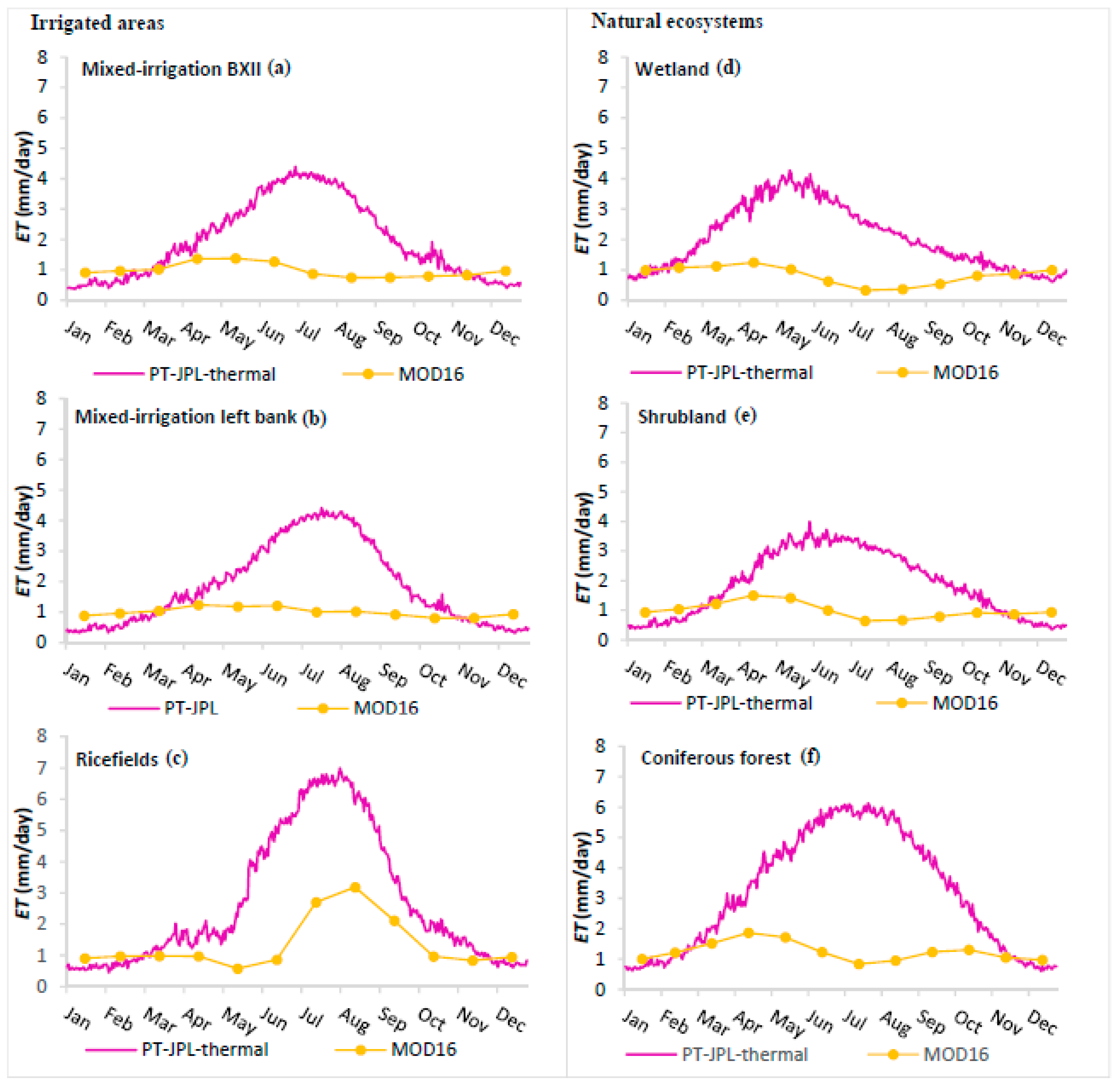
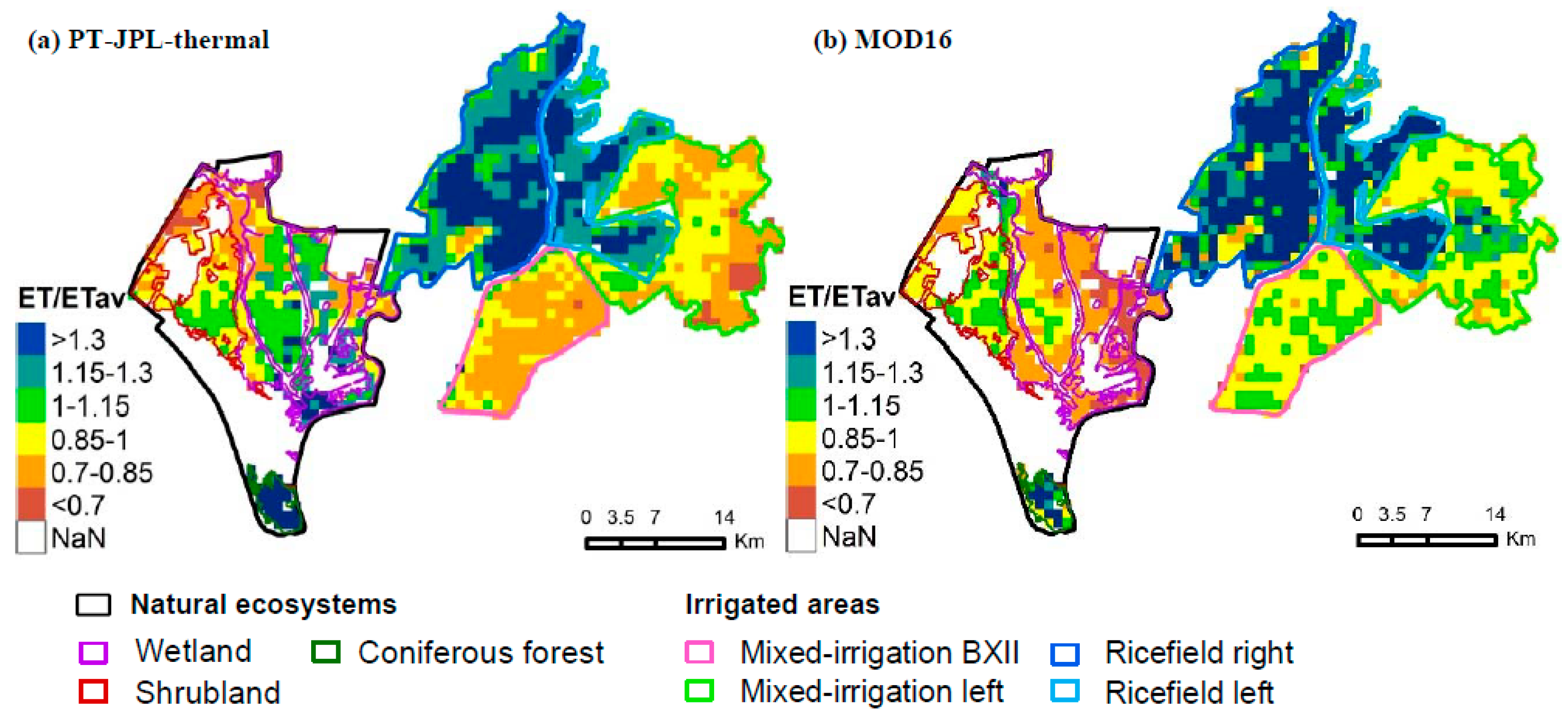
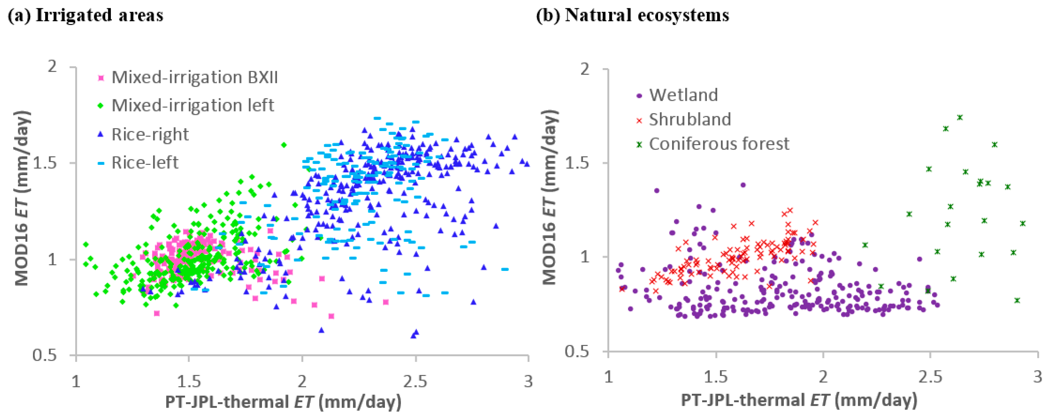
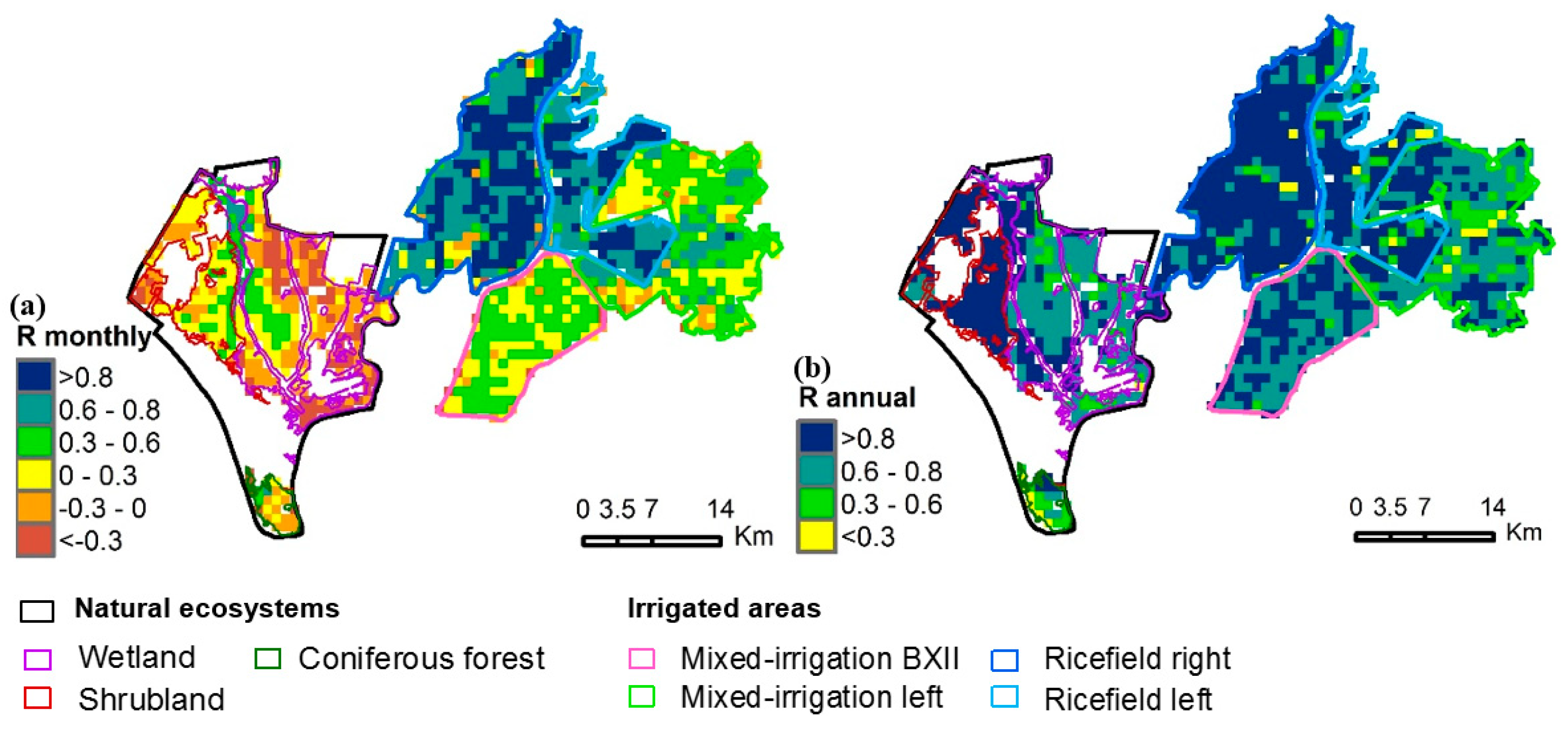
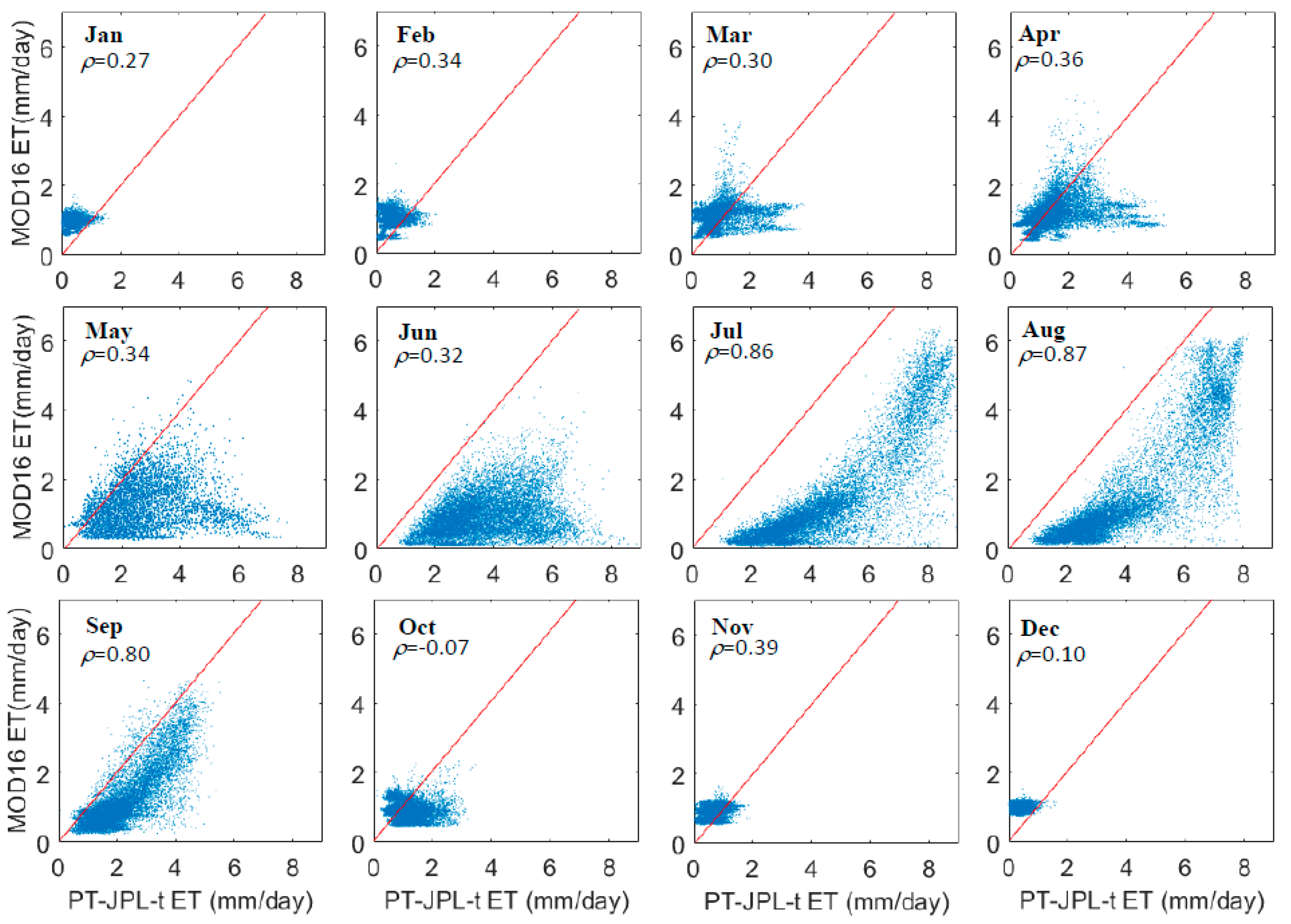
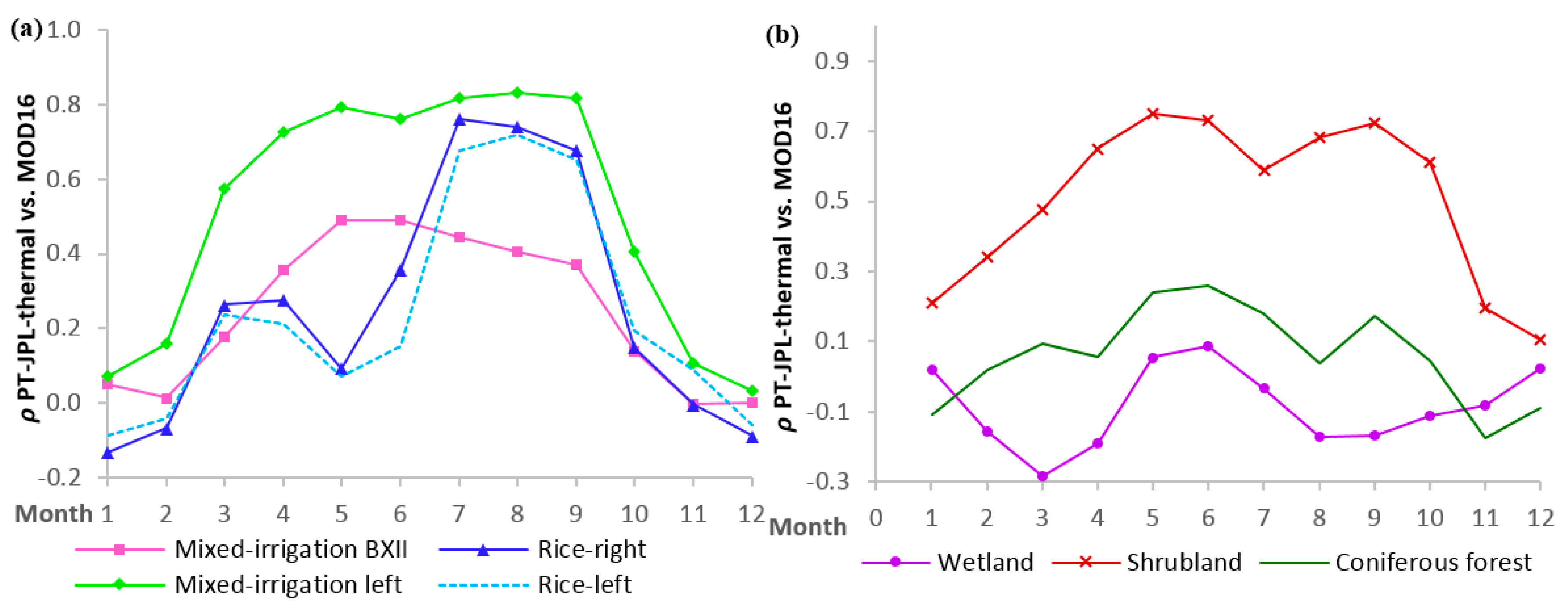
4.2. Assessment of PT-JPL-Thermal vs. MOD16 ET in the Doñana Region

From 2003 to 2012, the average evapotranspiration ET_av in the region including irrigated areas and natural ecosystems was estimated in 657 mm/year and 379 mm/year by the PT-JPL-thermal and MOD16, respectively. MOD16 reached 58% of the PT-JPL-thermal estimated ET_av. The monthly average ET in the region, which is shown in Figure 5a, showed a low correlation (ρ ≅ 0.48) and a large bias = −23.6 mm between models for a number of pairs n_p = 120 months. At an annual time-scale for a n_p = 10 years, the agreement between models increased (ρ ≅ 0.94, p < 0.001) and the bias remained large (see Figure 5b).

In the Doñana region, MOD16 showed a systematic negative bias with respect to the PT-JPL-thermal estimation for all the land cover classes. In addition, the timing of the peak intra-annual ET values did not coincide between models (Figure 6). The mixed-irrigation lands shown in Figure 6a,b presented maximum ET values in the summer (June to August) for the PT-JPL-thermal and spring (April to May) for MOD16. The rice fields presented maximum ET values from July to August for both the PT-JPL-thermal and MOD16 (Figure 6c). In the natural ecosystems, the PT-JPL-thermal showed maximum ET values in May for the wetland (Figure 6d), in June for the shrubland (Figure 6e), and in July for the coniferous forest (Figure 6f) while MOD16 detected maximum ET values in April for the three natural ecosystems.

The spatial patterns of the normalized ET values (ET/ET_av) in Figure 7 showed high agreement between models in which both depict the areas with higher and lower ET rates accordingly except for the wetland. Both models identified the higher normalized ET values in the rice fields and coniferous forests, and identified ET values close to the region average ET_av in the mixed-irrigation areas and shrublands. However, a significant disagreement between both models was found in the ET for the wetland. It resulted well above and below the ET_av in the region in the estimations derived from the PT-JPL-thermal and MOD16, respectively.

The scatterplots in Figure 8a,b show the relationship between the multi-year daily average ET estimations derived from the PT-JPL-thermal and MOD16 over the period from 2003 to 2012, which differentiate by irrigated areas and natural ecosystems. The correlation was found significant in the irrigated areas with ρ = 0.74 (p < 0.001) and a bias = −0.73 mm/day. In contrast, the correlation values were low in the natural ecosystems with ρ = 0.17 (p < 0.01) and a bias = −0.90 mm/day except for the shrubland, which showed a correlation value ρ = 0.68 (p < 0.001) and a bias of −0.59 mm/day.

Figure 9a,b show the temporal correlation values between model estimations at seasonal (months) and inter-annual scales. Higher correlation values were found in the inter-annual ET dynamics compared to the seasonal correlations.

The scatterplots in Figure 10 show the relationships between the PT-JPL-thermal and MOD16 ET estimations for all the land covers grouped for each month (n_p = 12,720 i.e., 1272 pixels in 10 years). Significantly higher correlation values were found in the summer months (i.e., July, August, and September) than in the period from October to March while the rest of the months did not show any significant correlation.

This information is complemented by Figure 11a,b, which show specific correlation values for each month and land cover class.

A high significant correlation was found in the irrigated areas during the months of maximum water demand (Figure 11a). In the natural ecosystems, a non-significant correlation was found (Figure 11b). Particularly for the wetland, the correlation coefficient was ρ = 0.07 with p = 0.25. For the coniferous forests, the correlation coefficient was ρ = −0.04 with p = 0.86. However, a significant correlation was observed in the shrubland during the spring and summer months (ρ > 0.7).

5. Discussion

5.1. Validation of the PT-JPL-Thermal ET

The ET derived from the PT-JPL-thermal showed, for all the estimators proposed (Table 3), a better performance than the estimated ET from MOD16 in which the high bias obtained indicates a significant underestimation of ET rates. Moreover, significant differences were observed in the ET dynamics between models with non-coincident timing of the peak annual values.

The PT-JPL-thermal ET dynamics at a monthly scale (Table 3) showed satisfactory agreement with WATEN ET and better results with the WATEN one-month lag. WATEN is a finite differences model run in one-month discrete time intervals whose inputs data may induce a lag in its calculation. Additionally, due to in-field irrigation data not available for modeling, WATEN uses water transfer data to the reservoir that stores the water to be applied as irrigation in the BXII [65]. All this introduces uncertainty regarding the time scale. The amount of variance and the e₂ coefficient indicate that the PT-JPL-thermal model is able to accurately capture the ET dynamics. However, MOD16 e₂ negative values suggest a high variance in the residuals which, together with the high values of the calculated errors, indicate a low capability for reproducing the WATEN ET dynamics. In addition, the Theil’s distribution components of the ET estimations (Table 4) obtained with the PT-JPL-thermal were close to ideal. With a low bias, there is well-represented variance and non-systematic residual errors in the ET estimations. For MOD16, the Theil’s inequality components distribution showed a poor model performance under our Mediterranean conditions.

When considering the average seasonality in the ET dynamics (Table 3), the PT-JPL-thermal estimates showed better results than the ET dynamics at a monthly scale with a higher amount of variance explained and smaller errors. On the other hand, the WATEN ET seasonality was not accurately represented by MOD16, which showed a similar e₂ coefficient and error values than those obtained at a monthly scale over the whole study period.

Since potential ET values estimated by Penman-Monteith (used in MOD16) and Priestley-Taylor (used in the PT-JPL-thermal) were similar (Figure 4), it could be assumed that differences between meteorological data sets used in the two RS models were negligible. This points out to the downscaling process from potential to actual ET as the source of disagreement, i.e., the use of the VPD (by MOD16) instead of the thermal approach (by the PT-JPL-thermal) to downscale to ET. With regard to semiarid irrigated areas, high values of VPD may reflect the surrounding arid conditions but do not take into account the real values of water availability [42]. Similar conclusions were achieved by Cicuéndez et al. [71] when comparing MODIS GPP with EC-derived GPP showing the importance of water availability apart from VPD. In addition, MOD16 considers the surface of the soil covered by water to be zero when RH is less than 70%. RH records were below 70% over the irrigation season from 2003 to 2012 at the agro-climatic station Lebrija I and, in consequence, MOD16 assumed the wet surface fraction as non-existent, which led to an underestimation of ET. Likewise, Biggs et al. [38] found the evaporative fraction from the irrigated cotton (the major cultivated crop in the mixed-irrigation BXII) to be underestimated in 67%. The significant correlation between the PT-JPL-thermal and WATEN ET estimations proved that the use of the thermal inertia concept as a proxy indicator of moisture status together with the re-formulation of the outgoing longwave radiation makes it possible to reproduce the dynamics of ET under our Mediterranean conditions in a more accurate manner than using the VPD alone.

5.2. Assessment of PT-JPL-Thermal vs. MOD16 ET in the Doñana Region

In the whole Doñana region, MOD16 estimations were also significantly lower than the PT-JPL-thermal ET values (Figure 5). Yet, a high agreement between models’ ET estimation was found in the whole region inter-annual dynamics (Figure 5b) and at a pixel level (Figure 9b) with ρ values around 0.8 in most of the pixels. As previously found by Mu et al. [72], although VPD alone may fail to capture the seasonality of water stress in some areas (Figure 9a), the inter-annual variability of water stress could be captured by VPD alone in most areas (Figure 9b), which indicated the adaptation of this approach for inter-annual global studies [72].

The PT-JPL-thermal ET estimations reasonably approached documented ET rates in the region per land cover class. The mixed-irrigation areas were found to evapotranspirate 4–5 mm/day in the summertime by using the PT-JPL-thermal approach (Figure 6a,b) in accordance with the on-site calibrated WATEN ET estimations in the mixed-irrigation BXII. In the rice fields, the irrigation supply is documented to be 6.3 mm/day on average in a five-month crop-cycle [73], which is reasonably approached by the PT-JPL-thermal ET estimations (Figure 6c). Previous studies [74] in Mediterranean-climate wetlands showed similar ET average values than those estimated by the PT-JPL-thermal from May to October (i.e., 6 mm/day with σ = 1.9 mm/day vs. 4 mm/day), which indicates that MOD16 may be underestimating evaporative fluxes (Figure 6d). Penatti et al. [75] obtained similar results in the world’s largest wetland (Pantanal) with a significant ET underestimation after winter and spring rainfall-periods. For the shrubland, (Figure 6e) MOD16 may underestimate ET due to a land use characterized as poorly vegetated surfaces, which is seen in previous findings in the Central Great Plains of the United Sates [37]. Although MOD16 has been documented to overestimate ET in forested areas over the Northeast Asia monsoon region [36,76], it was found to underestimate ET for coniferous forests under Mediterranean conditions as well (Figure 6f).

Intra-annual dynamics derived from the PT-JPL-thermal ET coincided with on-site irrigation management and natural ecosystems patterns in the region, while MOD16 ET presented some inconsistencies. The two mixed-irrigation areas (BXII and left bank) showed maximum MOD16 ET values in April contrary to the irrigation-patterns in the region (June to August), which were more accurately identified by the PT-JPL-thermal approach (Figure 6a,b). For the rice fields, both MOD16 and the PT-JPL-thermal identified maximum ET values in July and August (Figure 6c) according to the rice fields management in the region, which involves a five-month cultivation-cycle from May to September after which plots are drained and rice is harvested in October [73]. In the natural ecosystems, maximum PT-JPL-thermal ET fluxes were observed when the evaporative demand from the atmosphere ETp was high and when water was available and easily accessible. The PT-JPL-thermal was able to capture the natural ecosystems different ET patterns depending on their capability to access water. Therefore, the wetland ET dynamics were accurately captured (Figure 6d), showing the highest ET fluxes in April-May when water is available after rainfall and vegetation sprouts [77]. Our results match ET intra-annual dynamics previously documented by Drexler et al. [74] in a similar Mediterranean-climate wetland in the Sacramento-San Joaquin Delta in California. For the shrubland (Figure 6e), maximum rates were observed later in the spring (i.e., around June) coincident with the spring green-up period, which is supported by deep infiltration of winter and early spring precipitation, which was previously observed by Nagler et al. [78] in semiarid shrublands. In the coniferous forest, (Figure 6f) maximum ET values occurred later in the summer (i.e., July–August), which coincided with maximum ETp values and showed their root capability to access deeper soil moisture layers [79]. On the contrary, MOD16 showed the maximum ET values in April and the lowest ET values in July for the three ecosystems equally since this model relies on large-scale meteorological variables to estimate ET and is not able to capture ecosystems differences. In addition, the lowest ET values identified by MOD16 in July indicate the low capability of this model to assess ET fluxes in dry atmospheres with adequate soil moisture availability [33]. Since MOD16 bases the soil evaporation on RH and VPD alone, it does not take into account the availability of water in deep layers accessible for the shrublands’ and forests’ roots during part of the summer. This is especially important in the Doñana region because of the presence of the aquifer Almonte-Marismas on which the region rests, which assures water availability for some natural vegetation.

The ET spatial patterns derived from both model estimations clearly depict the land use distribution in the region with a significant agreement between models except in the wetland (Figure 7) where MOD16 ET values were lower than the average values in the region while the PT-JPL-thermal ET values were higher. MOD16 uses a land cover map for parameterization and, therefore, a differentiation of land uses was expected. The fact that the land use map does not include a wetland class may partially explain the low ET rates in this area. In addition, the RH criterion used in MOD16 [34] results in an erroneous elimination of the surface water cover fraction from April to October in the study region (RH below 70%). However, the PT-JPL-thermal is able to capture the distinct moisture dynamics among land cover classes accurately, which produces spatially consistent values within land uses and identifies large differences among them (Figure 7). This indicates that the physical concept of thermal inertia is applicable to different patterns of moisture availability such as areas with free water surfaces, irrigated crops, and natural vegetation extracting the water from deep layers.

Within land uses, the correlation of the multi-year average ET between the models at the pixel level was relatively high (ρ = 0.74) in the irrigated areas (Figure 8a) while, in the natural ecosystems, the agreement was much lower (ρ = 0.17) (Figure 8b). In the irrigated areas, despite the ET underestimation by MOD16, both methods seem to differentiate pixels with more and less evaporation accordingly (Figure 8a). However, the two models do not coincide in identifying the pixels with higher and lower ET values in the natural ecosystems especially in the wetland (Figure 8b). The availability of water for natural ecosystems due to the underlying Almonte-Marismas aquifer might be better captured by the thermal inertia approach used by the PT-JPL-thermal than with the HR and VPD approach used by MOD16. In addition, higher correlation values (ρ > 0.80) were found in the months of maximum water demand and high evapotranspiration from July to September (Figure 10). In particular, the rice fields and mixed-irrigation left bank showed the highest agreement in these months (Figure 11) in contrast to the natural ecosystems (except for the shrubland). A possible explanation is that the land cover product used by MOD16 to constrain ET values depending on land use is correctly assigned to the shrublands but fails in the wetland (classified as grassland) and coniferous forest (classified as permanent wetland and grassland).

6. Conclusions

We compared two RS evapotranspiration models in natural ecosystems and irrigated lands within the UNESCO protected Doñana Mediterranean region from 2003 to 2012. The intensification of human activity in the surroundings protected areas jeopardizes the effectiveness of these areas for preventing the degradation of natural ecosystems. RS-based evapotranspiration models provide a valuable tool for assessing human pressures and the risk of natural ecosystems collapse. We validated the ET estimates obtained from the modified PT-JPL model (PT-JPL-thermal) that introduces land surface temperature (LST) with a thermal inertia approach as a proxy to the soil moisture status against the on-site calibrated hydrological model WATEN and compared inter and intra-annual ET patterns with the globally available product MOD16 ET. The PT-JPL-thermal was found to reasonably reproduce the ET dynamics under our Mediterranean conditions (ρ = 0.78, ρ_{1-month lag} = 0.94) in contrast to MOD16 ET estimates, which pointed to poor model performance in the region. We found that MOD16 would allow us (i) to easily identify land uses with the lowest and largest water use and (ii) to assess inter-annual variability of ET in water-limited regions. However, the large negative bias (58% underestimation) found on MOD16 ET estimations in the evaluated land uses (irrigated areas plus natural ecosystems: wetland, shrubland, coniferous forest) would not allow MOD16 to approach the ET quantification under water-limited conditions. The PT-JPL-thermal reasonably approached ET rates in the region, revealing well-differentiated and coherent spatio-temporal patterns among the evaluated land uses. This study has proven that the use of the thermal inertia concept as a proxy indicator to soil moisture status, together with the re-formulation of the outgoing longwave radiation, is capable of reproducing ET at a regional level in semiarid environments. This requires only air temperature and incoming solar radiation from climatic databases apart from standard satellites and products freely available for ET estimations. In addition, this study highlights the potentiality to estimate ET of a simpler model less vulnerable to the uncertainties of multiple types of forcing data in comparison to more theoretically accurate models that require complex parameters difficult to characterize globally.

References

1. Prudhomme, C.; Giuntoli, I.; Robinson, E.L.; Clark, D.B.; Arnell, N.W.; Dankers, R.; Fekete, B.M.; Franssen, W.; Gerten, D.; Gosling, S.N. Hydrological droughts in the 21st century, hotspots and uncertainties from a global multimodel ensemble experiment. Proc. Natl. Acad. Sci. USA 2014, 111, 3262–3267. [Google Scholar] [CrossRef] [PubMed] [Green Version]
2. Alexandratos, N.; Bruinsma, J. World Agriculture towards 2030/2050: The 2012 Revision; ESA Working Paper; FAO: Rome, Italy, 2012. [Google Scholar]
3. Schewe, J.; Heinke, J.; Gerten, D.; Haddeland, I.; Arnell, N.W.; Clark, D.B.; Dankers, R.; Eisner, S.; Fekete, B.M.; Colón-González, F.J. Multimodel assessment of water scarcity under climate change. Proc. Natl. Acad. Sci. USA 2014, 111, 3245–3250. [Google Scholar] [CrossRef] [PubMed] [Green Version]
4. Flörke, M.; Schneider, C.; McDonald, R.I. Water competition between cities and agriculture driven by climate change and urban growth. Nat. Sustain. 2018, 1, 51–58. [Google Scholar] [CrossRef]
5. Curtis, S.; Gamble, D.W.; Popke, J. Sensitivity of crop water need to 2071–95 projected temperature and precipitation changes in Jamaica. Earth Interact. 2014, 18, 1–17. [Google Scholar] [CrossRef]
6. Hoerling, M.; Eischeid, J.; Perlwitz, J.; Quan, X.; Zhang, T.; Pegion, P. On the increased frequency of Mediterranean drought. J. Clim. 2012, 25, 2146–2161. [Google Scholar] [CrossRef]
7. Tanasijevic, L.; Todorovic, M.; Pereira, L.S.; Pizzigalli, C.; Lionello, P. Impacts of climate change on olive crop evapotranspiration and irrigation requirements in the Mediterranean region. Agric. Water Manag. 2014, 144, 54–68. [Google Scholar] [CrossRef]
8. Diffenbaugh, N.S.; Pal, J.S.; Giorgi, F.; Gao, X. Heat stress intensification in the Mediterranean climate change hotspot. Geophys. Res. Lett. 2007, 34, 224–228. [Google Scholar] [CrossRef]
9. Minacapilli, M.; Consoli, S.; Vanella, D.; Ciraolo, G.; Motisi, A. A time domain triangle method approach to estimate actual evapotranspiration: Application in a Mediterranean region using MODIS and MSG-SEVIRI products. Remote Sens. Environ. 2016, 174, 10–23. [Google Scholar] [CrossRef]
10. Lambin, E.F.; Turner, B.L.; Geist, H.J.; Agbola, S.B.; Angelsen, A.; Bruce, J.W.; Coomes, O.T.; Dirzo, R.; Fischer, G.; Folke, C. The causes of land-use and land-cover change: Moving beyond the myths. Glob. Environ. Chang. 2001, 11, 261–269. [Google Scholar] [CrossRef]
11. Chavez-Jimenez, A.; Granados, A.; Garrote, L.; Martín-Carrasco, F. Adapting water allocation to irrigation demands to constraints in water availability imposed by climate change. Water Resour. Manag. 2015, 29, 1413–1430. [Google Scholar] [CrossRef]
12. Scanlon, B.R.; Jolly, I.; Sophocleous, M.; Zhang, L. Global impacts of conversions from natural to agricultural ecosystems on water resources: Quantity versus quality. Water Resour. Res. 2007, 43, 215–222. [Google Scholar] [CrossRef]
13. Oki, T.; Kanae, S. Global hydrological cycles and world water resources. Science 2006, 313, 1068–1072. [Google Scholar] [CrossRef] [PubMed]
14. Chirouze, J.; Boulet, G.; Jarlan, L.; Fieuzal, R.; Rodriguez, J.; Ezzahar, J.; Raki, S.E.; Bigeard, G.; Merlin, O.; Garatuza-Payan, J. Intercomparison of four remote-sensing-based energy balance methods to retrieve surface evapotranspiration and water stress of irrigated fields in semi-arid climate. Hydrol. Earth Syst. Sci. Discuss. 2014, 1165–1188. [Google Scholar] [CrossRef] [Green Version]
15. Leuning, R.; Zhang, Y.; Rajaud, A.; Cleugh, H.; Tu, K. A simple surface conductance model to estimate regional evaporation using MODIS leaf area index and the Penman-Monteith equation. Water Resour. Res. 2008, 44, 652–655. [Google Scholar] [CrossRef]
16. Allen, R.G.; Pereira, L.S.; Howell, T.A.; Jensen, M.E. Evapotranspiration information reporting: I. Factors governing measurement accuracy. Agric. Water Manag. 2011, 98, 899–920. [Google Scholar] [CrossRef]
17. Anderson, M.C.; Kustas, W.P.; Norman, J.M. Upscaling and downscaling—A regional view of the soil–plant–atmosphere continuum. Agron. J. 2003, 95, 1408–1423. [Google Scholar] [CrossRef]
18. Wang, K.; Dickinson, R.E.; Wild, M.; Liang, S. Evidence for decadal variation in global terrestrial evapotranspiration between 1982 and 2002: 1. Model development. J. Geophys. Res. Atmos. 2010, 115. [Google Scholar] [CrossRef] [Green Version]
19. Song, L.; Zhuang, Q.; Yin, Y.; Zhu, X.; Wu, S. Spatio-temporal dynamics of evapotranspiration on the Tibetan Plateau from 2000 to 2010. Environ. Res. Lett. 2017, 12, 014011. [Google Scholar] [CrossRef] [Green Version]
20. Guzinski, R.; Nieto, H.; Stisen, S.; Fensholt, R. Inter-comparison of energy balance and hydrological models for land surface energy flux estimation over a whole river catchment. Hydrol. Earth Syst. Sci. 2015, 19, 2017–2037. [Google Scholar] [CrossRef] [Green Version]
21. Xing, W.; Wang, W.; Shao, Q.; Yu, Z.; Yang, T.; Fu, J. Periodic fluctuation of reference evapotranspiration during the past five decades: Does Evaporation Paradox really exist in China? Sci. Rep. 2016, 6, 39503. [Google Scholar] [CrossRef] [PubMed] [Green Version]
22. Fisher, J.B.; Melton, F.; Middleton, E.; Hain, C.; Anderson, M.; Allen, R.; McCabe, M.F.; Hook, S.; Baldocchi, D.; Townsend, P.A. The future of evapotranspiration: Global requirements for ecosystem functioning, carbon and climate feedbacks, agricultural management, and water resources. Water Resour. Res. 2017, 53, 2618–2626. [Google Scholar] [CrossRef] [Green Version]
23. Senay, G.; Leake, S.; Nagler, P.; Artan, G.; Dickinson, J.; Cordova, J.; Glenn, E. Estimating basin scale evapotranspiration (ET) by water balance and remote sensing methods. Hydrol. Process. 2011, 25, 4037–4049. [Google Scholar] [CrossRef]
24. Beven, K.; Freer, J. Equifinality, data assimilation, and uncertainty estimation in mechanistic modelling of complex environmental systems using the GLUE methodology. J. Hydrol. 2001, 249, 11–29. [Google Scholar] [CrossRef]
25. Fortin, V.; Chahinian, N.; Montanari, A.; Moretti, G.; Moussa, R. Distributed hydrological modelling with lumped inputs. IAHS Publ. 2006, 307, 135. [Google Scholar]
26. Olioso, A.; Chauki, H.; Courault, D.; Wigneron, J.-P. Estimation of evapotranspiration and photosynthesis by assimilation of remote sensing data into SVAT models. Remote Sens. Environ. 1999, 68, 341–356. [Google Scholar] [CrossRef]
27. Xu, X.; Li, J.; Tolson, B.A. Progress in integrating remote sensing data and hydrologic modeling. Prog. Phys. Geogr. 2014, 38, 464–498. [Google Scholar] [CrossRef]
28. Yilmaz, M.T.; Anderson, M.C.; Zaitchik, B.; Hain, C.R.; Crow, W.T.; Ozdogan, M.; Chun, J.A.; Evans, J. Comparison of prognostic and diagnostic surface flux modeling approaches over the Nile River basin. Water Resour. Res. 2014, 50, 386–408. [Google Scholar] [CrossRef] [Green Version]
29. Kalma, J.D.; McVicar, T.R.; McCabe, M.F. Estimating land surface evaporation: A review of methods using remotely sensed surface temperature data. Surv. Geophys. 2008, 29, 421–469. [Google Scholar] [CrossRef]
30. Karimi, P.; Bastiaanssen, W.G. Spatial evapotranspiration, rainfall and land use data in water accounting—Part 1: Review of the accuracy of the remote sensing data. Hydrol. Earth Syst. Sci. 2015, 19, 507–532. [Google Scholar] [CrossRef]
31. Monteith, J.L. Evaporation and environment. Symp. Soc. Exp. Biol. 1965, 19, 205–234. [Google Scholar] [PubMed]
32. Allen, R.G.; Pereira, L.S.; Raes, D.; Smith, M. Crop Evapotranspiration—Guidelines for Computing Crop Water Requirements; FAO Irrigation and Drainage Paper 56; FAO: Rome, Italy, 1998; Volume 300, p. D05109. [Google Scholar]
33. Mu, Q.; Heinsch, F.A.; Zhao, M.; Running, S.W. Development of a global evapotranspiration algorithm based on MODIS and global meteorology data. Remote Sens. Environ. 2007, 111, 519–536. [Google Scholar] [CrossRef]
34. Mu, Q.; Zhao, M.; Running, S.W. Improvements to a MODIS global terrestrial evapotranspiration algorithm. Remote Sens. Environ. 2011, 115, 1781–1800. [Google Scholar] [CrossRef]
35. Zhang, Y.; Leuning, R.; Hutley, L.B.; Beringer, J.; McHugh, I.; Walker, J.P. Using long-term water balances to parameterize surface conductances and calculate evaporation at 0.05° spatial resolution. Water Resour. Res. 2010, 46. [Google Scholar] [CrossRef] [Green Version]
36. Hu, G.; Jia, L.; Menenti, M. Comparison of MOD16 and LSA-SAF MSG evapotranspiration products over Europe for 2011. Remote Sens. Environ. 2015, 156, 510–526. [Google Scholar] [CrossRef]
37. Velpuri, N.M.; Senay, G.B.; Singh, R.K.; Bohms, S.; Verdin, J.P. A comprehensive evaluation of two MODIS evapotranspiration products over the conterminous United States: Using point and gridded FLUXNET and water balance ET. Remote Sens. Environ. 2013, 139, 35–49. [Google Scholar] [CrossRef]
38. Biggs, T.W.; Marshall, M.; Messina, A. Mapping daily and seasonal evapotranspiration from irrigated crops using global climate grids and satellite imagery: Automation and methods comparison. Water Resour. Res. 2016, 52, 7311–7326. [Google Scholar] [CrossRef]
39. Priestley, C.; Taylor, R. On the assessment of surface heat flux and evaporation using large-scale parameters. Mon. Weather Rev. 1972, 100, 81–92. [Google Scholar] [CrossRef]
40. Zhang, K.; Kimball, J.S.; Mu, Q.; Jones, L.A.; Goetz, S.J.; Running, S.W. Satellite based analysis of northern ET trends and associated changes in the regional water balance from 1983 to 2005. J. Hydrol. 2009, 379, 92–110. [Google Scholar] [CrossRef]
41. Fisher, J.B.; Tu, K.P.; Baldocchi, D.D. Global estimates of the land–atmosphere water flux based on monthly AVHRR and ISLSCP-II data, validated at 16 FLUXNET sites. Remote Sens. Environ. 2008, 112, 901–919. [Google Scholar] [CrossRef]
42. García, M.; Sandholt, I.; Ceccato, P.; Ridler, M.; Mougin, E.; Kergoat, L.; Morillas, L.; Timouk, F.; Fensholt, R.; Domingo, F. Actual evapotranspiration in drylands derived from in-situ and satellite data: Assessing biophysical constraints. Remote Sens. Environ. 2013, 131, 103–118. [Google Scholar] [CrossRef]
43. Muñoz-Reinoso, J.C. Doñana mobile dunes: What is the vegetation pattern telling us? J. Coast. Conserv. 2018, 1–10. [Google Scholar] [CrossRef]
44. García De Jalón, S.; Iglesias, A.; Cunningham, R.; Díaz, J.I.P. Building resilience to water scarcity in southern Spain: A case study of rice farming in Doñana protected wetlands. Reg. Environ. Chang. 2014, 14, 1229–1242. [Google Scholar] [CrossRef]
45. Martín-López, B.; García-Llorente, M.; Palomo, I.; Montes, C. The conservation against development paradigm in protected areas: Valuation of ecosystem services in the Doñana social–ecological system (southwestern Spain). Ecol. Econom. 2011, 70, 1481–1491. [Google Scholar] [CrossRef]
46. Green, A.J.; Bustamante, J.; Janss, G.F.E.; Fernández-Zamudio, R.; Díaz-Paniagua, C. Doñana Wetlands (Spain). In The Wetland Book II: Distribution, Description and Conservation; Finlayson, C.M., Milton, R., Prentice, C., Davidson, N.C., Eds.; Springer: Dordrecht, The Netherlands, 2017. [Google Scholar]
47. Serrano, L.; Diaz-Paniagua, C.; Gomez-Rodriguez, C.; Florencio, M.; Marchand, M.A.; Roelofs, J.G.; Lucassen, E.C. Susceptibility to acidification of groundwater-dependent wetlands affected by water level declines, and potential risk to an early-breeding amphibian species. Sci. Total Environ. 2016, 571, 1253–1261. [Google Scholar] [CrossRef] [PubMed]
48. García-Novo, F.; Marín-Cabrera, C. Doñana: Water and Biosphere; Doñana 2005, Confederación Hidrográfica del Guadalquivir; Ministerio de Medio Ambiente: Seville, Spain, 2006.
49. Estévez, J.; Gavilán, P.; García-Marín, A. Data validation procedures in agricultural meteorology—A prerequisite for their use. Adv. Sci. Res. 2011, 6, 141–146. [Google Scholar] [CrossRef]
50. Purdy, A.; Fisher, J.; Goulden, M.; Famiglietti, J. Ground heat flux: An analytical review of 6 models evaluated at 88 sites and globally. J. Geophys. Res. Biogeosci. 2016, 121, 3045–3059. [Google Scholar] [CrossRef]
51. Jackson, R.; Hatfield, J.; Reginato, R.; Idso, S.; Pinter, P., Jr. Estimation of daily evapotranspiration from one time-of-day measurements. Agric. Water Manag. 1983, 7, 351–362. [Google Scholar] [CrossRef]
52. García, M.; Villagarcía, L.; Contreras, S.; Domingo, F.; Puigdefábregas, J. Comparison of three operative models for estimating the surface water deficit using ASTER reflective and thermal data. Sensors 2007, 7, 860–883. [Google Scholar] [CrossRef]
53. Bisht, G.; Venturini, V.; Islam, S.; Jiang, L. Estimation of the net radiation using MODIS (Moderate Resolution Imaging Spectroradiometer) data for clear sky days. Remote Sens. Environ. 2005, 97, 52–67. [Google Scholar] [CrossRef]
54. Potter, C.S.; Randerson, J.T.; Field, C.B.; Matson, P.A.; Vitousek, P.M.; Mooney, H.A.; Klooster, S.A. Terrestrial ecosystem production: A process model based on global satellite and surface data. Glob. Biogeochem. Cycles 1993, 7, 811–841. [Google Scholar] [CrossRef]
55. Yuan, W.; Liu, S.; Yu, G.; Bonnefond, J.-M.; Chen, J.; Davis, K.; Desai, A.R.; Goldstein, A.H.; Gianelle, D.; Rossi, F. Global estimates of evapotranspiration and gross primary production based on MODIS and global meteorology data. Remote Sens. Environ. 2010, 114, 1416–1431. [Google Scholar] [CrossRef] [Green Version]
56. Peters, J.; De Baets, B.; De Clercq, E.M.; Ducheyne, E.; Verhoest, N.E. The potential of multitemporal Aqua and Terra MODIS apparent thermal inertia as a soil moisture indicator. Int. J. Appl. Earth Obs. Geoinf. 2011, 13, 934–941. [Google Scholar]
57. Mitra, D.; Majumdar, T. Thermal inertia mapping over the Brahmaputra basin, India using NOAA-AVHRR data and its possible geological applications. Int. J. Remote Sens. 2004, 25, 3245–3260. [Google Scholar] [CrossRef]
58. Verstraeten, W.W.; Veroustraete, F.; van der Sande, C.J.; Grootaers, I.; Feyen, J. Soil moisture retrieval using thermal inertia, determined with visible and thermal spaceborne data, validated for European forests. Remote Sens. Environ. 2006, 101, 299–314. [Google Scholar] [CrossRef]
59. Norman, J.M.; Kustas, W.P.; Humes, K.S. Source approach for estimating soil and vegetation energy fluxes in observations of directional radiometric surface temperature. Agric. For. Meteorol. 1995, 77, 263–293. [Google Scholar] [CrossRef]
60. IFAPA. Estación Meteorológica de Lebrija I. Available online: http://www.juntadeandalucia.es/agriculturaypesca/ifapa/ria/servlet/FrontController?action=Static&url=fechas.jsp&c_provincia=41&c_estacion=3 (accessed on 7 March 2017).
61. Idso, S.B.; Jackson, R.D. Thermal radiation from the atmosphere. J. Geophys. Res. 1969, 74, 5397–5403. [Google Scholar] [CrossRef]
62. Parton, W.J.; Logan, J.A. A model for diurnal variation in soil and air temperature. Agric. Meteorol. 1981, 23, 205–216. [Google Scholar] [CrossRef]
63. Rasmussen, M.O.; Sørensen, M.K.; Wu, B.; Yan, N.; Qin, H.; Sandholt, I. Regional-scale estimation of evapotranspiration for the North China Plain using MODIS data and the triangle-approach. Int. J. Appl. Earth Obs. Geoinf. 2014, 31, 143–153. [Google Scholar] [CrossRef]
64. Iqbal, M. An Introduction to Solar Radiation; Academic Press: Toronto, ON, USA, 1983. [Google Scholar]
65. Moyano, M.C.; Tornos, L.; Juana, L. Water balance and flow rate discharge on a receiving water body: Application to the B-XII Irrigation District in Spain. J. Hydrol. 2015, 527, 38–49. [Google Scholar] [CrossRef]
66. Cleugh, H.A.; Leuning, R.; Mu, Q.; Running, S.W. Regional evaporation estimates from flux tower and MODIS satellite data. Remote Sens. Environ. 2007, 106, 285–304. [Google Scholar] [CrossRef]
67. Nash, J.E.; Sutcliffe, J.V. River flow forecasting through conceptual models part I—A discussion of principles. J. Hydrol. 1970, 10, 282–290. [Google Scholar] [CrossRef]
68. Moriasi, D.N.; Arnold, J.G.; Van Liew, M.W.; Bingner, R.L.; Harmel, R.D.; Veith, T.L. Model evaluation guidelines for systematic quantification of accuracy in watershed simulations. Trans. ASABE 2007, 50, 885–900. [Google Scholar] [CrossRef]
69. Pindyck, R.S.; Rubinfeld, D.L. Econometric Models and Economic Forecasts; Irwin/McGraw-Hill: Boston, MA, USA, 1998; Volume 4. [Google Scholar]
70. Watson, P.K.; Teelucksingh, S.S. A Practical Introduction to Econometric Methods: Classical and Modern; University of West Indies Press: Mona, West Indies, 2002. [Google Scholar]
71. Cicuéndez, V.; Rodríguez-Rastrero, M.; Huesca, M.; Uribe, C.; Schmid, T.; Inclán, R.; Litago, J.; Sánchez-Girón, V.; Merino-de-Miguel, S.; Palacios-Orueta, A. Assessment of soil respiration patterns in an irrigated corn field based on spectral information acquired by field spectroscopy. Agric. Ecosyst. Environ. 2015, 212, 158–167. [Google Scholar] [CrossRef]
72. Mu, Q.; Zhao, M.; Heinsch, F.A.; Liu, M.; Tian, H.; Running, S.W. Evaluating water stress controls on primary production in biogeochemical and remote sensing based models. J. Geophys. Res. Biogeosci. 2007, 112, 863–866. [Google Scholar] [CrossRef]
73. JdA. El cultivo del arroz en Andalucía. Secretaría general de Agricultura, Ganadería y Desarrollo Rural, España. Available online: https://www.juntadeandalucia.es/agriculturaypesca/portal/export/sites/default/comun/galerias/galeriaDescargas/cap/servicio-estadisticas/Estudios-e-informes/agricultura/herbaceos-extensivos/arr07121.pdf (accessed on 7 March 2017).
74. Drexler, J.Z.; Anderson, F.E.; Snyder, R.L. Evapotranspiration rates and crop coefficients for a restored marsh in the Sacramento–San Joaquin Delta, California, USA. Hydrol. Process. 2008, 22, 725–735. [Google Scholar] [CrossRef]
75. Penatti, N.C.; de Almeida, T.I.R.; Ferreira, L.G.; Arantes, A.E.; Coe, M.T. Satellite-based hydrological dynamics of the world’s largest continuous wetland. Remote Sens. Environ. 2015, 170, 1–13. [Google Scholar] [CrossRef]
76. Jang, K.; Kang, S.; Lim, Y.J.; Jeong, S.; Kim, J.; Kimball, J.S.; Hong, S.Y. Monitoring daily evapotranspiration in Northeast Asia using MODIS and a regional Land Data Assimilation System. J. Geophys. Res. Atmos. 2013, 118, 1277. [Google Scholar] [CrossRef]
77. Ontillera, R.R.; González-Nóvoa, J.A. Marismas de Doñana. Ecosistemas de Doñana; MAPAMA: Madrid, Spain.
78. Nagler, P.; Glenn, E.; Kim, H.; Emmerich, W.; Scott, R.; Huxman, T.; Huete, A. Relationship between evapotranspiration and precipitation pulses in a semiarid rangeland estimated by moisture flux towers and MODIS vegetation indices. J. Arid Environ. 2007, 70, 443–462. [Google Scholar] [CrossRef]
79. Garcia, M.; Fernandez, N.; Gonzalez-Dugo, M.P.; Delibes, M. Impact of Annual Drought on the Water and Energy Exchanges in the Doñana Region (SW Spain). In Proceedings of the Symposium Earth Observation and Water Cycle Science, Frascati, Italy, 18–20 November 2009. [Google Scholar]
Figure 1. Map of the study area including (i) irrigated areas: mixed-irrigation areas (BXII District and left bank) and rice fields, (ii) natural ecosystems in the Doñana National Park: wetland, shrubland, and coniferous forest.
Remotesensing 10 01105 g001
Figure 2. (a) Monthly ET (mm/day), (b) average ET seasonality (mm/day), (c) annual ET (mm/year) derived from WATEN, PT-JPL-thermal, and MOD16 in the mixed-irrigation BXII for the period between 2003 to 2012.
Remotesensing 10 01105 g002
Figure 3. Scatterplot of monthly ET (mm/day) from the PT-JPL-thermal and MOD16 versus WATEN ET in the mixed-irrigation BXII.
Remotesensing 10 01105 g003
Figure 4. (a) Monthly ETp (mm/day) derived from the agro-climatic station Lebrija I versus ETp from the PT-JPL-thermal and MOD16 over 2003 to 2012. (b) Average monthly correlation of ETp (mm/day) from PT-JPL-thermal and MOD16 against ETp at Lebrija I.
Remotesensing 10 01105 g004
Figure 5. (a) Region-averaged ETav (mm/day), (b) region-averaged ETav (mm/year) derived from the PT-JPL-thermal and MOD16 in the study region (irrigated areas plus natural ecosystems) from 2003 to 2012.
Remotesensing 10 01105 g005
Figure 6. PT-JPL-thermal and MOD16 ET seasonality over the period between 2003 to 2012. (ac) in the irrigated areas (rice fields and mixed-irrigated lands) and (df) in the natural ecosystems (wetland, shrubland and coniferous forest).
Remotesensing 10 01105 g006
Figure 7. Normalized ET values: ET/ETav where ET is the multiyear average ET per pixel and ETav is the average ET within the region over the period between 2003 to 2012. (a) PT-JPL-thermal ETav = 1.81 mm/day and (b) MOD16 ETav = 1.03 mm/day.
Remotesensing 10 01105 g007
Figure 8. PT-JPL-thermal vs. MOD16 multi-year average ET estimations (mm/day) in (a) the irrigated areas and (b) the natural ecosystems.
Remotesensing 10 01105 g008
Figure 9. Temporal correlation between PT-JPL-thermal and MOD16 (a) seasonal (np = 120, 120 months per pixel), (b) inter-annual (np = 10, 10 years per pixel).
Remotesensing 10 01105 g009
Figure 10. Monthly ET (mm/month) from PT-JPL-thermal vs. MOD16 in the study region (irrigated areas plus natural ecosystems), np = 12,720 (1272 region-pixels in 10 years from 2003–2012).
Remotesensing 10 01105 g010
Figure 11. Correlation coefficients of the PT-JPL-thermal vs. MOD16 ET monthly patterns from 2003 to 2012 for: (a) the irrigated areas and (b) the natural ecosystems.
Remotesensing 10 01105 g011