Assessing the Pattern Differences between Satellite-Observed Upper Tropospheric Humidity and Total Column Water Vapor during Major El Niño Events

Abstract

As part of the activities for the Global Energy and Water Exchanges (GEWEX) water vapor assessment project, the consistency of satellite-observed upper tropospheric humidity (UTH) and total column water vapor (TCWV) is examined. The examination is focused on their respective patterns during major El Niño events. The analysis shows that the two datasets, consisting of one measurement of vertically averaged relative humidity in the upper troposphere and one of absolute water vapor integrated over the atmospheric vertical column with dominant contribution from the lower troposphere, are consistent over the equatorial central–eastern Pacific, both showing increases of water vapor during major El Niño events as expected. However, the magnitude of drying in the TCWV field over the western Pacific is much weaker than that of moistening over the central–eastern Pacific, while the UTH field exhibits equivalent magnitude of drying and moistening. Furthermore, the drying in the UTH field covers larger areas in the tropics. The difference in their patterns results in an opposite phase in the time series during a major El Niño event when a tropical average is taken. Both UTH and TCWV are closely correlated with major climate indices. However, they have significantly different lag correlations with the Niño 3.4 index in both the sign (positive or negative) and lag time over tropical oceans.

1. Introduction

A water vapor assessment was initiated by the Global Energy and Water Exchanges (GEWEX) project (hereafter, the GEWEX water vapor assessment is abbreviated as G-VAP) to intercompare and evaluate three essential climate variables (ECVs) of water vapor, including total column water vapor (TCWV), upper tropospheric humidity (UTH), and profiles of water vapor. The TCWV and profiles of water vapor datasets have been widely used by the science community for weather and climate studies. An inventory of these datasets submitted to and analyzed by G-VAP is available at http://gewex-vap.org/?page_id=13. The UTH datasets submitted to G-VAP include satellite observations from the High-Resolution Infrared Radiation Sounder (HIRS), the Advanced Microwave Sounding Unit B (AMSU-B) and Microwave Humidity Sounder (MHS), and the Meteosat Visible and InfraRed Imager (MVIRI) and Spinning Enhanced Visible and InfraRed Imager (SEVIRI). Though the amount of UTH accounts for only a very small portion of TCWV, it is a significant absorption source of the outgoing longwave radiation, and thus UTH has a profound impact in the climate feedback processes [1,2,3]. The G-VAP assessment covers evaluations of both the overall characteristics of participating data records for each of these ECVs and the consistency among ECVs. The first phase of G-VAP concluded in 2017 with a report to the World Climate Research Programme (WCRP) [4]. Many related research works and assessments have advanced our understanding of water vapor measurements from satellite sensors and their general advantages and limitations for climate applications; see, for example, [5,6,7,8,9,10].

As we enter the second phase of the assessment with new versions and extended time series of datasets, the present study updates and expands on the analysis of the consistency between satellite-derived UTH and TCWV variables as part of the G-VAP activities. Noting that TCWV is largely weighted by water vapor in the lower troposphere, an analysis between UTH and TCWV shows how the distribution of water vapor in the upper troposphere differs from that in the lower troposphere and what aspects are consistent between the two measurements. During major El Niño events, tropical water vapor fields exhibit distinct characteristics. The enhanced signals facilitate the examination of datasets. El Niño and La Niña are the warm and cold phases, respectively, of the El Niño–Southern Oscillation (ENSO). The Southern Oscillation describes a bimodal variation in sea level barometric pressure between observation stations at Darwin, Australia and Tahiti. Normally, lower pressure over Darwin and higher pressure over Tahiti sustains easterly trade winds. An El Niño event is associated with the weakening of the easterly trade winds and the warming of ocean water in the central and eastern equatorial Pacific. During El Niño events, the western Pacific often experiences drought, while heavy precipitation occurs in the coastal region of equatorial South America [11]. Through teleconnection, the occurrences of El Niño and La Niña events have major influences on the weather and climate around the world. For example, recent studies found that the ENSO phase has an influence on the annual cycle characteristics of United States tornadoes [12]. El Niño events tend to dry southern Africa in various patterns and magnitudes of precipitation anomalies, with strong El Niño events resulting in rainfall deficits often less than −0.88 standardized units [13]. The response of China’s hydroclimate anomalies to a strong El Niño event is significant via El Niño and warm Indian Ocean-induced circulation anomalies [14]. The ENSO has a strong impact on the total northern hemispheric polar cold air mass amount below a potential temperature of 280 K [15].

The two longest-available climate data records (CDRs) of satellite observations for UTH and TCWV that are submitted to G-VAP are examined in this study. These are the HIRS UTH and the Hamburg Ocean Atmosphere Parameters and Fluxes from Satellite Data (HOAPS) datasets, respectively. Both datasets are derived from fundamental CDRs that are available at public domains. The UTH and TCWV variations are closely associated with the ENSO [6,9,16,17,18,19,20,21]. As an integral part of atmospheric systems, distributions of UTH and TCWV are governed by the large-scale atmospheric circulations. Atmospheric water vapor is closely related to anomalies in sea surface temperature (SST) through the Clausius–Clapeyron equation; see, for example, [9,22]. ENSO events are commonly defined by anomalies of SST, and an examination of corresponding changes in the UTH and TCWV contributes to a fuller picture of the atmospheric systems during these events.

Within G-VAP, the UTH assessment includes intercomparisons of UTH, assessments on variability of UTH datasets, and consistency comparisons of UTH with other water vapor datasets. Global UTH has been routinely measured by satellite sensors. The HIRS sounders have been observing UTH since 1978. The MVIRI and SEVIRI from geostationary satellites have collected data since 1983. Microwave measurement of UTH started in 1998 with AMSU-B and then MHS. New measurements have been added in recent years with hyperspectral sounders including the Atmospheric Infrared Sounder (AIRS), Infrared Atmospheric Sounding Interferometer (IASI), and Cross-Track Infrared Sounder (CrIS). Efforts in developing upper tropospheric water vapor datasets from different satellite sensors established the climatology of UTH [17,23,24,25,26,27], and further studies advanced our understanding of its variability [16,21,28,29,30,31]. UTH datasets have been used in numerous studies that cover a wide variety of topics. It has been shown that the moistening of UTH plays a key role in the feedback mechanism for amplifying anthropogenic climate change [32,33,34]. The HIRS UTH channel measurements were combined with other satellite datasets to analyze the climatological interactions between deep convection, upper-tropospheric humidity, and atmospheric greenhouse trapping [35]. UTH measurements supported other observations in detecting the changes of large-scale tropical circulations that define the Hadley and Walker circulations [36] and tropical width [37]. The focus of the present study is to investigate the variability patterns of UTH compared to those of TCWV during ENSO events as part of the G-VAP assessment.

The results reported in this article represent a subset of the assessment activities, that is, the consistency assessment between satellite-derived HIRS UTH and HOAPS TCWV, in the second phase of the G-VAP analyses. In the first phase, a consistency comparison was performed using an older version of the TCWV dataset (version 3.2 of HOAPS) over the time period of 1988–2009 [4]. In the second phase, the HIRS UTH patterns are compared to a new version of HOAPS (version 4.0) to reveal their similarities and differences in variability patterns for an extended common time period of 1988–2014. In the following, Section 2 describes datasets used. Section 3 discusses variability patterns for both UTH and TCWV datasets. Conclusions are provided in Section 4.

2. Dataset Specifications

The HIRS is a sensor carried by the National Oceanic and Atmospheric Administration (NOAA) series of satellites and by the Meteorological operational satellite (MetOp) - A and - B. The HIRS UTH data are derived from the HIRS Channel 12 CDR version v3.0 from the National Centers for Environmental Information (NCEI), available at https://www.ncdc.noaa.gov/cdr/fundamental/hirs-ch12-brightness-temperature. The data record’s digital object identifier (DOI) is located at https://0-doi-org.brum.beds.ac.uk/10.7289/V5N58JC9. Data were processed to correct limb-effect and to clear cloudy pixels [38]. Observations from different satellites have been intercalibrated to a reference satellite, for which NOAA-12 is designated [17]. The operational HIRS sensors underwent three major designs. Sensors with designs 2, 3, and 4 have been flown on nine, three, and four satellites, respectively. The HIRS sensor on NOAA-12 was a HIRS/2 sensor. In choosing a reference satellite, several factors were considered, including that HIRS/2 instruments were on more than half of the satellites, that NOAA-12 had the second longest time series (NOAA-14 had the longest) among the HIRS/2 satellites, and that its orbital drift was relatively small (compared to NOAA-14). The upper tropospheric humidity (in the relative humidity unit of %) is calculated based on the relationship between UTH and HIRS channel 12 brightness temperatures (T_6.7) derived by Soden and Bretherton [39]:

$$UTH=\frac{cos\theta }{p_0}{e}^{\left(31.5-0.115T_{6.7}\right)}$$

(1)

in which $\theta$ is the viewing angle and $p_0$ is derived from the climatological values of the pressure of the 240 K isotherm divided by 300 hPa ($p_0$ = p[T = 240 K]/300 hPa). For limb-corrected data, the term cos$\theta$ is equal to one. The HIRS UTH dataset has a monthly global coverage based on clear-sky observations with a spatial resolution of 2.5° × 2.5° degrees, covering the period November 1978–December 2016.

The HOAPS set is a completely satellite-based climatology of precipitation, evaporation, and freshwater budget (evaporation minus precipitation) as well as related turbulent heat fluxes and atmospheric state variables including, among others, TCWV. All variables are derived from the Special Sensor Microwave Imager (SSM/I) and SSMI/Sounder (SSMIS) passive microwave radiometers onboard the Defence Meteorological Satellite Program satellites F08, F10, F11, F13, F14, F15, F16, F17, and F18, except for the SST, which is taken from Advanced Very High Resolution Radiometer (AVHRR) measurements [40]. SSM/I and SSMIS data has been carefully quality-controlled, recalibrated, and intercalibrated [41]. A general overview of HOAPS is given by Andersson et al. [42]. More specifically, TCWV is derived with a one-dimensional variational (1D-Var) retrieval scheme using SSM/I-like channels (19.35, 22.235, 37.0, and 85.5 GHz). Both horizontal and vertical polarizations of the channels are used as input, except for the 22.235 GHz channel, which measures only vertically polarized radiation. As background to the 1D-Var, the profiles database described in [43] is used. The physics of the retrieval are described in more detail in [44]. Details on the TCWV product quality can be found in, for example, [45]: it is characterized by a unique combination of stability and temporal coverage. The TCWV product from HOAPS has a global coverage, that is, within ±180° longitude and ±80° latitude, and is only defined over the ice-free ocean surface. The product is available as monthly averages and 6-hourly composites on a regular latitude/longitude grid with a spatial resolution of 0.5° × 0.5° degrees, of which the monthly data are used in the present study. HOAPS 4.0 covers the period July 1987–December 2014 and is DOI-referenced (10.5676/EUM_SAF_CM/HOAPS/V002 [46]).

3. Variability

3.1. Time Series

To show the temporal variation of UTH and TCWV during ENSO events, Figure 1 plots the time series of the two variables over ocean areas in 20°S–20°N. The upper panel shows monthly mean values of UTH and TCWV, and the lower panel shows the corresponding anomalies. The figure displays strong seasonal variations of both UTH and TCWV. Since the HIRS observation started in 1978, there were three major El Niño events, occurring in 1982–83, 1997–98, and 2015–16. The HOAPS TCWV time series covered one of these major events (1997–98). Significant changes during the major El Niño events in the time series are found in both UTH and TCWV.

Comparing UTH to TCWV time series, it is interesting to note that the phase of the UTH time series is mostly opposite to that of TCWV, especially during the one major El Niño event in the common period (1997–98 event). The contrast is a result of different characteristics in the two observations. During a major El Niño event, lower atmospheric water vapor significantly increases in the eastern Pacific and in several other regions through teleconnections associated with the increase of SST. The water vapor increase in the lower atmosphere is reflected by the positive TCWV anomalies over large areas of the tropics. During such an event, the increase of lower atmospheric water vapor facilitates the transport of water vapor to the upper troposphere. However, the increase of UTH is constrained to a relatively smaller region. Beyond the confined region, the water vapor in the upper troposphere dissipates, resulting in a smaller area of the positive UTH anomalies compared to that of positive TCWV anomalies in the tropics. The UTH field is more closely related to changes in both the ascending and descending branches of general circulations. Over the Pacific, changes in atmospheric circulations during an El Niño event can bring higher UTH to the central–eastern Pacific, but it also decreases UTH significantly in other tropical Pacific areas. Notably, UTH decreases in the western Pacific, where the strength of the ascending branch of the general circulation decreases, and in the subtropics, where the descending branches in both hemispheres strengthen. The areas of decreased UTH are larger than the areas where UTH increases. When an area average of UTH over the tropical zonal belt (20°S–20°N) is taken, it numerically results in negative anomalies. During several less major El Niño events in the analyzed common periods, that is, 2002–03, 2006–07, and 2009–10, negative anomalies in the zonal mean of UTH and positive anomalies in the zonal mean of TCWV (consistent with overall increases in SST) are also observed.

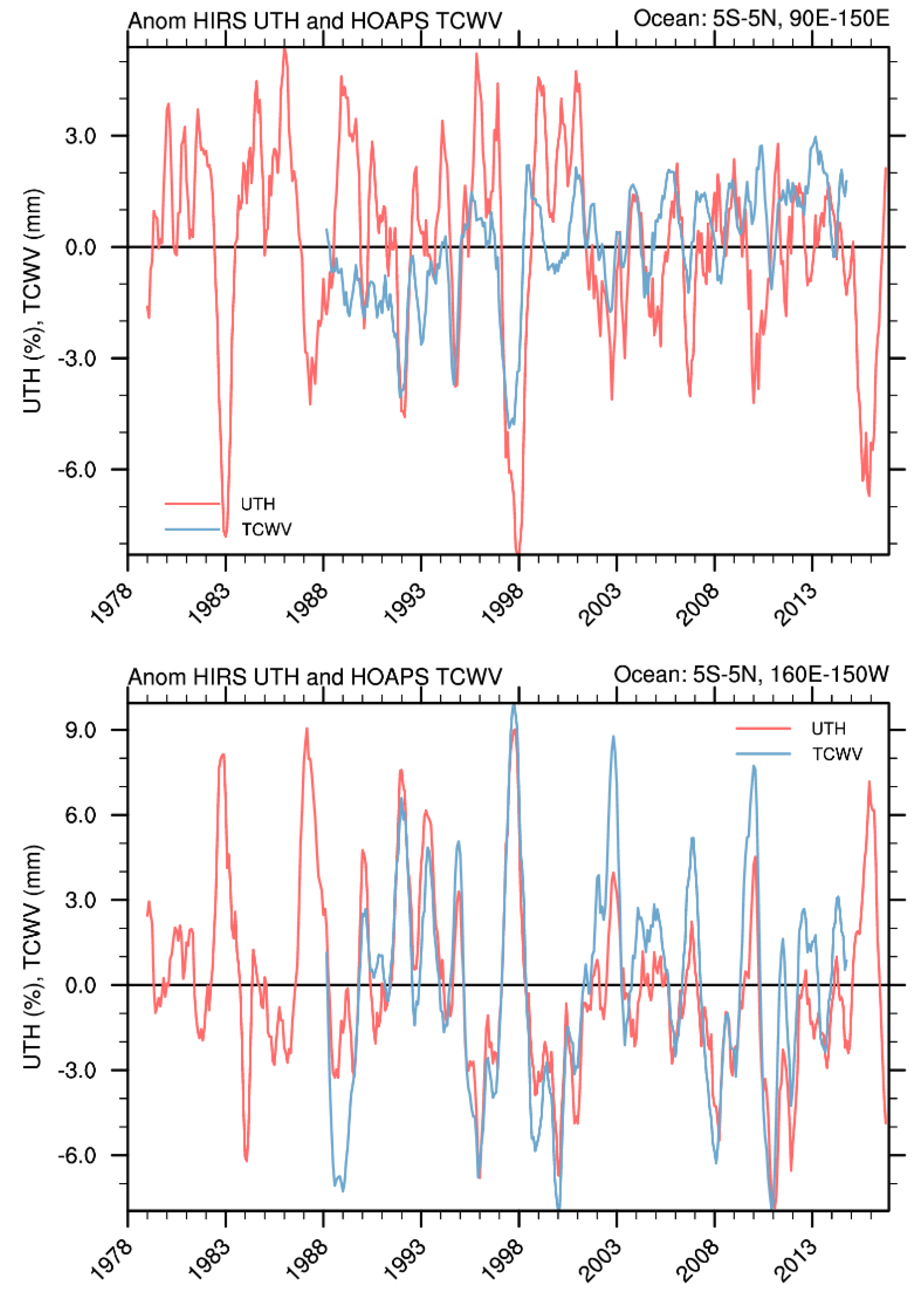
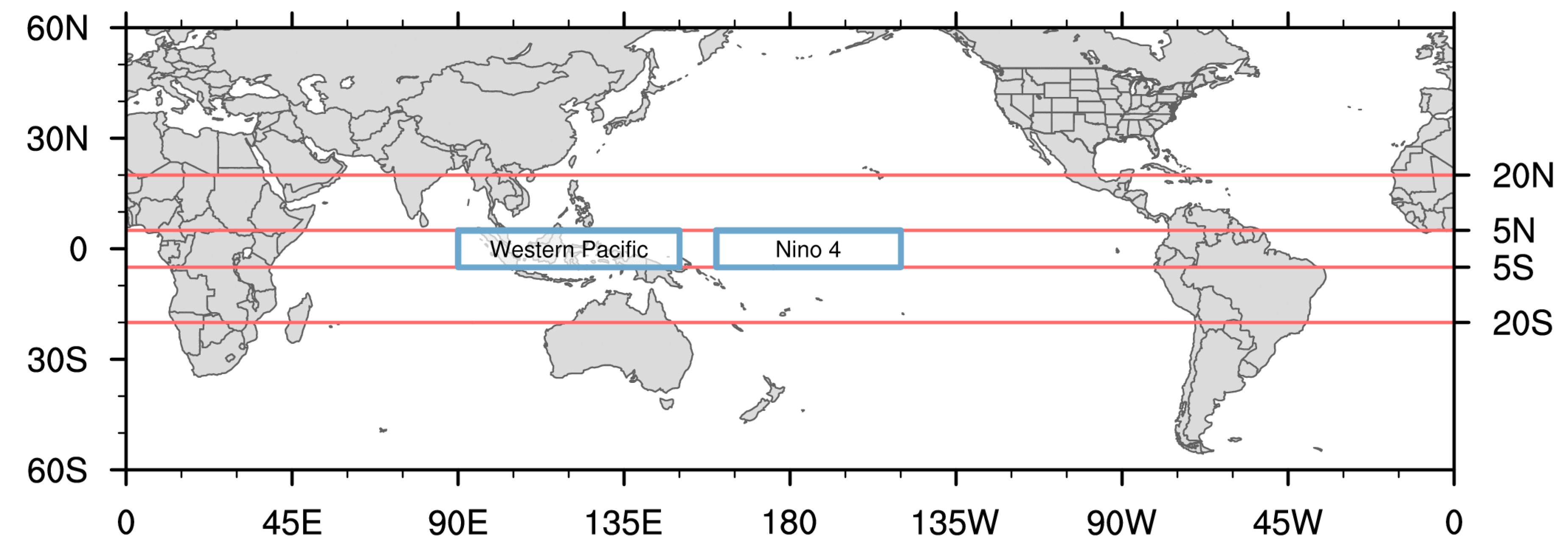
To further illustrate the regional variability of UTH, Figure 2 shows the time series of UTH and TCWV over the equatorial western and central Pacific for 5°S–5°N. The upper panel displays the area-averaged anomaly time series in the equatorial western Pacific between 90°E and 150°E, and the lower panel is the anomaly time series over the Niño 4 region. These two regions are mapped in Figure 3. When the averaging is reduced from the zonal to regional scale, the phase of the UTH time series is highly consistent with that of TCWV time series during ENSO events, especially over the Niño 4 region.

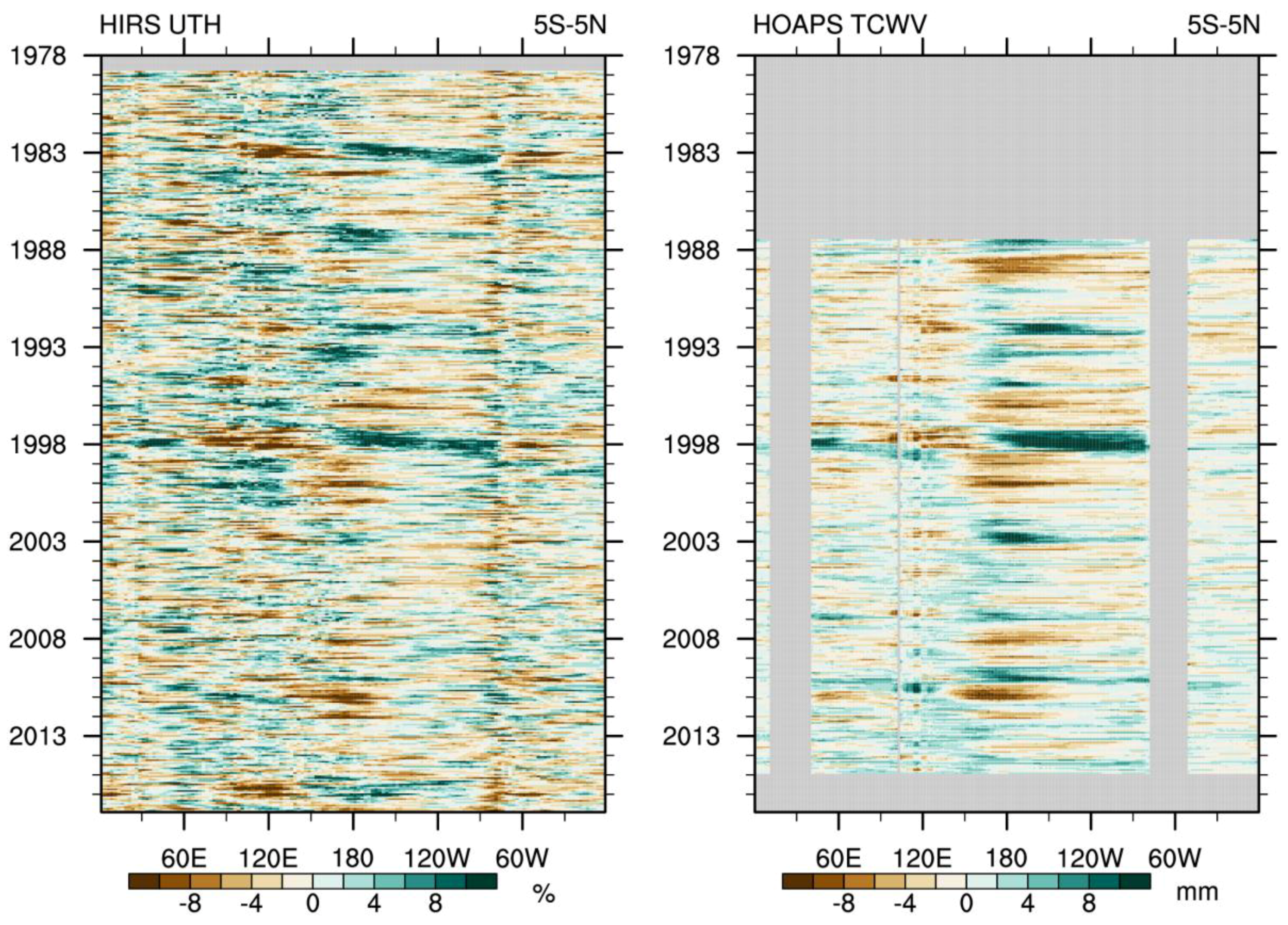
Hovmöller analysis is a useful tool in displaying details of spatial variability in a time series. Figure 4 shows longitude–time evolutions of monthly UTH (left panel) and TCWV (right panel) anomalies around the equator, averaged between 5°S and 5°N. The stripes near 30°E and 60°W in the TCWV panel indicate land surfaces over which TCWV data are unavailable. The onset of the 1997–98 El Niño, as defined by the Oceanic Niño Index (ONI) (calculated using the three-month running mean of Extended Reconstructed Sea Surface Temperature (ERSST) v5 [47] SST anomalies in the Niño 3.4 region (5°N–5°S, 120°–170°W)), started in May 1997. Both the TCWV and UTH series show that preceding this El Niño event (at the end of 1996), there was a positive anomaly of water vapor near the dateline. This is consistent with the finding of higher water vapor concentration in previous studies of the 1997–98 El Niño [48,49,50]. The studies linked the higher water vapor to a build-up of heat content in the atmosphere due to stronger-than-normal trade winds associated with a weak La Niña in 1995–96. Soon after the onset of the 1997–98 El Niño, positive anomalies of TCWV rapidly extended from the dateline to the eastern end of the equatorial Pacific. However, the shift of positive anomalies in the UTH field that started at the dateline to the eastern Pacific was more gradual through the course of the El Niño event, resulting in a lag behind the TCWV positive anomalies in the eastern Pacific. As the water vapor built up all the way from the lower atmosphere (implied by TCWV) to the upper troposphere (marked by UTH) at the peak of the El Niño, there was also a significantly increased water vapor mixing ratio at 215 hPa over the eastern Pacific [51], indicating that the deep convection extended to the tropopause. During the time of water vapor increase in the eastern Pacific, a dry region developed in the western Pacific in both the TCWV and UTH fields.

The UTH panel shows that the 1982–83 and 1997–98 El Niño events evolved in similar patterns, but the 2015–16 event was different from the earlier two major events. Unlike the previous events, there was a notable increase of water vapor at the eastern end of the Pacific for the 2015–16 event at about the same time as the onset of the UTH increase near the dateline. The overall intensity of the UTH increase in the 2015–16 event was not as strong as that in the previous two major events.

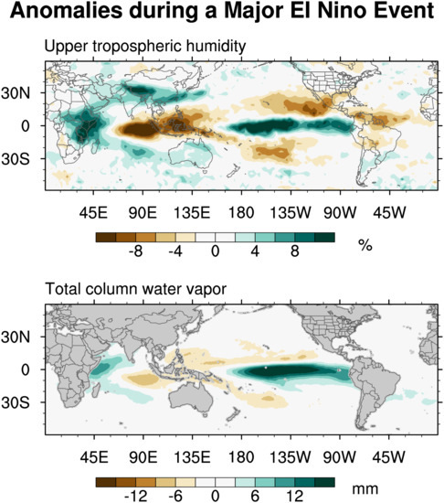
3.2. Anomalies during Major El Niño and La Niña Events

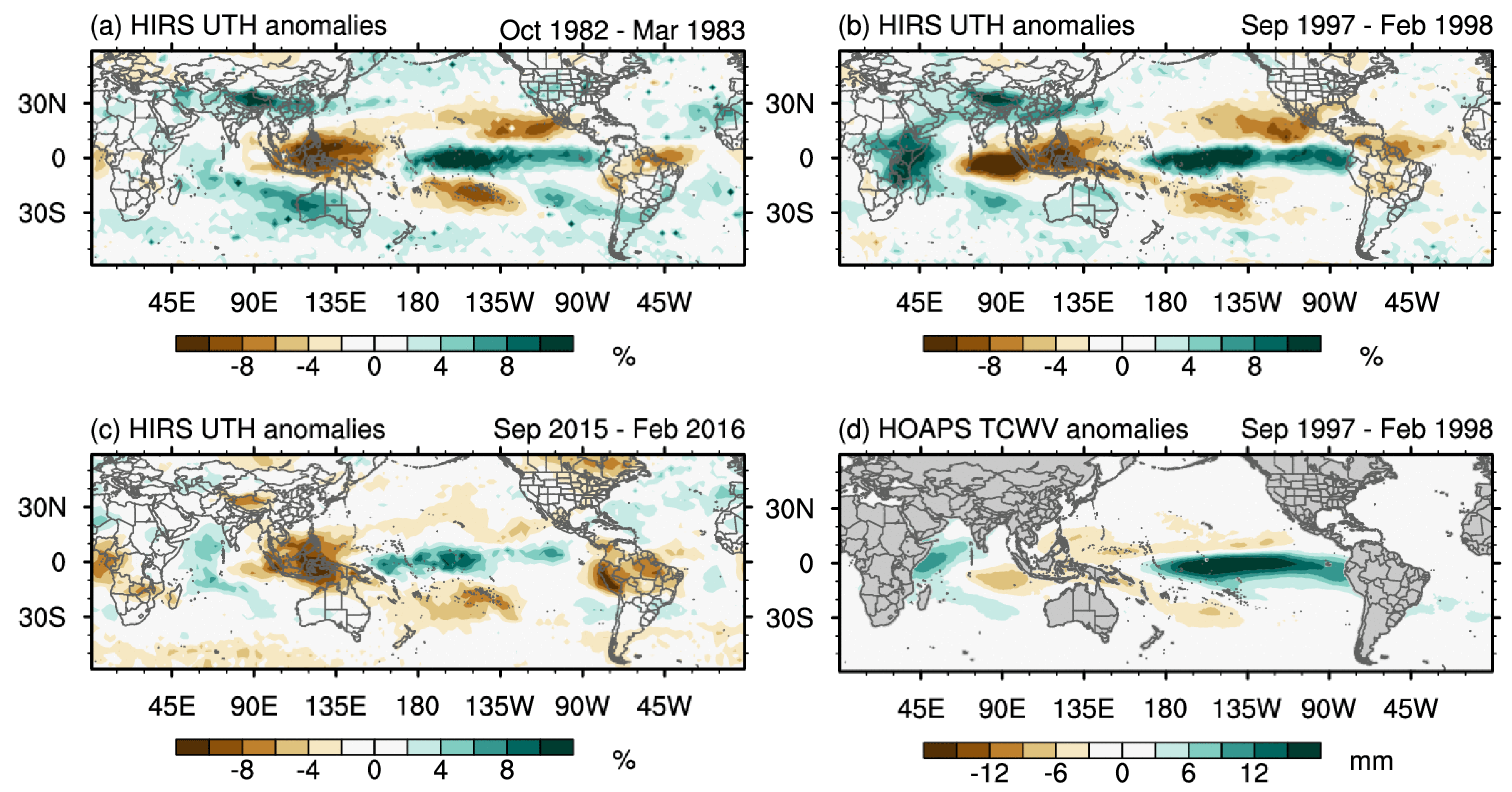
The spatial anomalies of UTH and TCWV during major El Niño and La Niña events are shown in Figure 5 and Figure 6. In the time series of the HIRS UTH, there were three very strong El Niño events (1982–83, 1997–98, and 2015–16). During these events, several SST anomaly indices, including the commonly used ONI, Niño 3 Index, Niño 3.4 Index, and Niño 4 Index, exceeded 2 °C. Figure 5a–c displays UTH anomalies averaged over six months in the peak of the three El Niño events, respectively. The six months are determined based on the largest anomalies in ONI (available at: http://www.cpc.ncep.noaa.gov/products/analysis_monitoring/ensostuff/ensoyears.shtml). Figure 5a–c shows that the three El Niño events all exhibited the strongest positive anomalies over the equatorial central Pacific, extending to the eastern Pacific. Compensating subsidence driven by the El Niño convection produced negative anomalies on each side of the positive anomalies. The equatorial Pacific’s positive anomalies were flanked to the north and south by negative anomalies over the subtropical Pacific from 10°–30°N and 10°–30°S. To the east and west, they were similarly coupled with negative anomalies over the western Pacific into the Indian Ocean and also over Brazil. Farther west, large positive anomalies covered extensive areas of the western Indian Ocean.

Despite similarities, differences are evident among the three El Niño events. The 1982–83 El Niño event produced significant positive UTH anomalies over southwestern Australia through teleconnection that were not matched by the other two events. The 1997–98 events had the strongest equatorial negative anomalies over the eastern Indian Ocean, and much larger positive anomalies over equatorial eastern Africa compared to the 1982–83 and 2015–16 events. The equatorial Pacific positive anomalies in the 2015–16 event were smaller than the earlier two major events. Its positive anomaly area at the eastern Pacific tilted to higher latitudes and the negative areas over the northern South America continent were more prominent.

Though the commonly used indicators of El Niño strength are mostly based on positive anomalies of SST in the equatorial central–eastern Pacific, other indicators, such as the Multivariate El Niño/Southern Oscillation Index (MEI), incorporate SST with additional measurements. The MEI index integrates sea-level pressure, zonal and meridional components of the surface wind, SST, surface air temperature, and total cloudiness fraction of the sky in the calculation [52]. The MEI time series (https://www.esrl.noaa.gov/psd/enso/mei/#data) shows that, among the three strongest El Niño events since 1950, the 1982–83 and 1997–98 events reached the MEI value 3.0, while the 2015–16 El Niño event’s MEI value was 2.5. This is reflected in the smaller positive anomalies found in the 2015–16 central–eastern Pacific UTH. A study on the characteristics of extreme El Niño events showed that the 2015–16 El Niño was marked by a record-breaking warm anomaly in the central Pacific, but was weaker in many measures than the two previous extreme El Niño events [53]. In another study [54] that compared the three El Niño events using reanalyses from the Modern-Era Retrospective Analysis for Research and Applications (MERRA) 2, it was found that the 2015–16 event had a shallower thermocline over the eastern Pacific with a weaker zonal contrast of subsurface water temperatures along the equatorial Pacific. Figure 5c shows that though the positive anomalies over the equatorial central–eastern Pacific were not as large as those in the 1982–83 and 1997–98 events, the negative (dry) anomalies over Indonesia were nearly as significant. In the austral spring of 2015, Indonesia experienced huge forest fires that caused a haze crisis in neighboring countries [53].

The shorter TCWV time series has coverage for the 1997–98 El Niño, one of the three events discussed above, and the anomaly field for this event is displayed in Figure 5d. The locations of positive and negative anomalies in the tropics are very similar to those in the UTH field; however, the positive anomalies over the central–eastern Pacific are significantly larger than the negative anomalies over Indonesia and the eastern Indian Ocean. The TCWV teleconnections are less pronounced compared to the UTH.

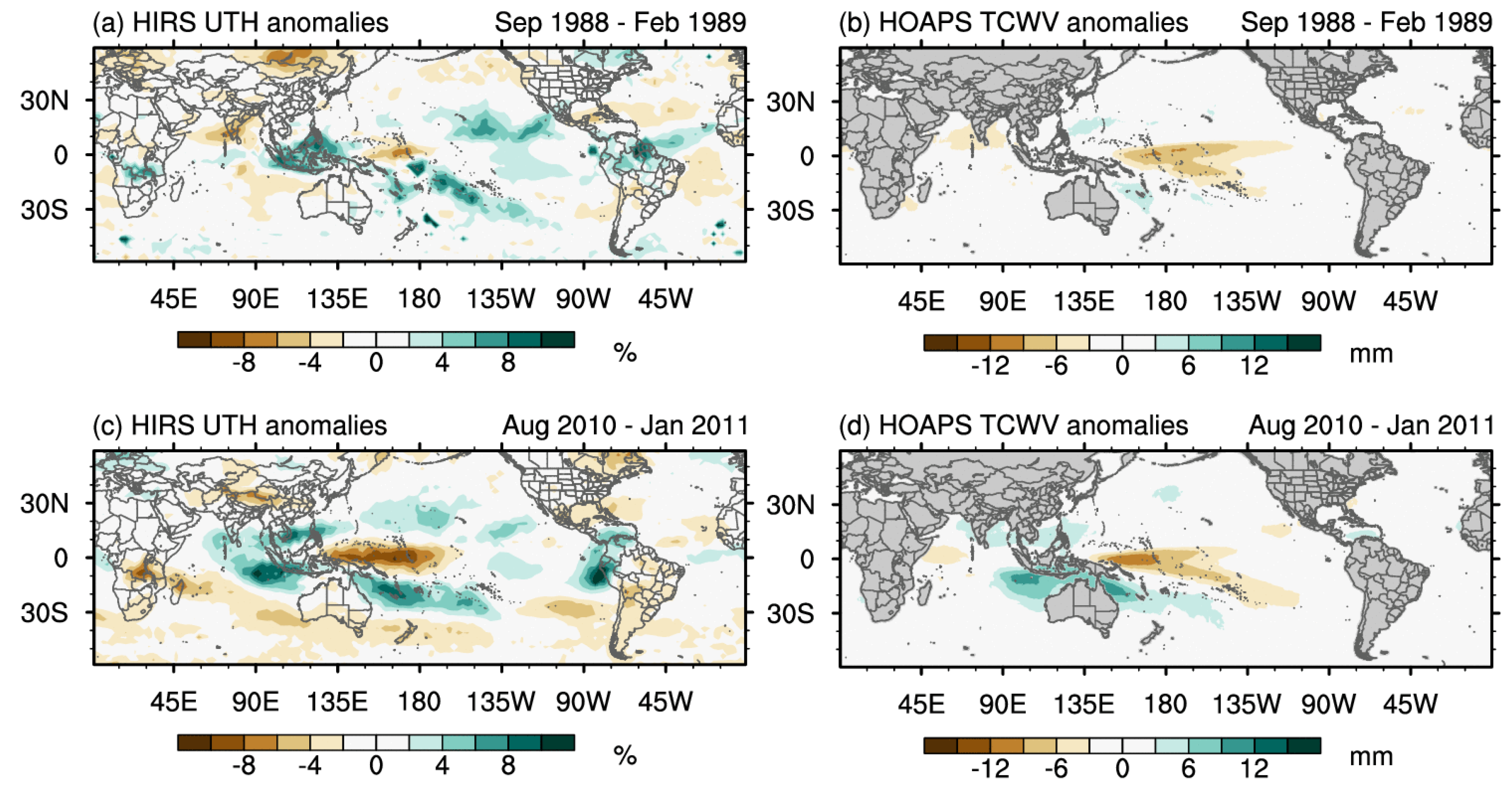
Figure 6 shows the anomaly fields averaged over six months near the peak of La Niña for two of the strong events during the common period of the UTH and TCWV time series. The 1988–89 event reached the ONI value of −1.8 and the MEI value of −1.5, and the 2010–11 event reached the two index values of −1.7 and −1.9, respectively. During La Niña events, the central Pacific and Indonesia exhibited mostly opposite anomaly patterns compared to the El Niño patterns depicted in Figure 5. La Niña events tend to lead to significant increases of UTH in the equatorial western Pacific and subtropics and decreases of UTH in the equatorial central Pacific. Either neutral or slightly positive UTH anomalies may be found in the equatorial eastern Pacific during these events. Such positive anomalies in this region are usually not present in the TCWV fields during strong La Niña events. Again, the TCWV teleconnections are less pronounced compared to the UTH. In general, the strength of La Niña, as depicted as UTH or TCWV anomalies, appears to be more consistent with MEI than with ONI.

3.3. Correlation Analysis

The UTH and TCWV variations are regulated by large-scale climate systems. The relationships can be highlighted by correlation analyses with indices that capture climate patterns in various regions of the globe and in various lengths of the phases [55]. The one-point (pairwise) correlation maps between water vapor datasets and two climate indices, namely, the Niño 3.4 and Pacific Decadal Oscillation (PDO), are computed to examine the variability in a climate context. Many studies have shown profound influences of these index phases on global and regional climates [6,56,57,58]. The correlations show how closely the UTH and TCWV distributions relate to the variables used in tracking the climate indices. The analysis also detects teleconnection patterns with climate indices in various regions of the world.

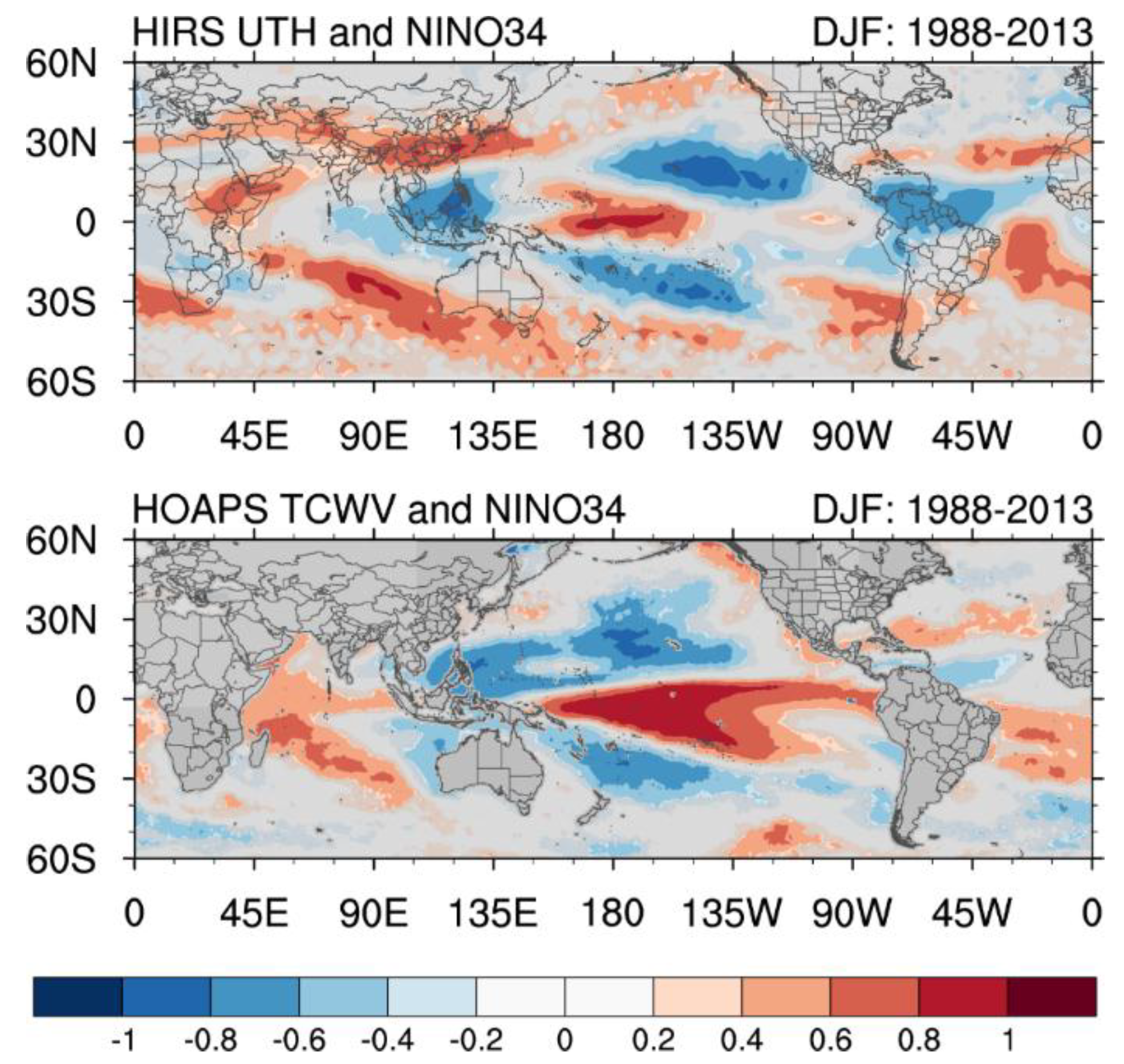
The Niño 3.4 index is based on the anomalies of SST of the region 5°N–5°S and 120–170°W, and it is often used to define El Niño and La Niña events [59]. Correlations between the time series of UTH at each grid point and the time series of the Niño 3.4 SST anomaly are displayed in the upper panel of Figure 7. Similarly, the correlations between TCWV and the Niño 3.4 SST anomaly are displayed in the lower panel. As the ENSO events are more active during the boreal winter season, the correlation maps for December, January, and February (DJF) are shown. The correlation pattern is linked to the mirrored effects of El Niño and La Niña. The upper panel of Figure 7 shows that over the tropics, the highest correlation (~0.8) between HIRS UTH and Niño 3.4 anomalies is over the central equatorial Pacific in the Niño 4 domain. Large correlations of the opposite sign are found over the western Pacific near Indonesia and in the subtropics: one at 20–30°N and another at 20–30°S over the Pacific. During El Niño events, these areas with negative correlations correspond to either weakened ascending branches of the atmospheric circulations (the western Pacific) or strengthened descending branches during El Niño. The increase in Niño 3.4 SST facilitates the transportation of more moisture into the upper troposphere over the central and eastern equatorial Pacific, while the subsidence may dry the upper troposphere over both the northern and southern subtropical Pacific. The opposite is often mirrored during La Niña events. The increase of SST in the eastern Pacific can affect regions outside of the tropics by altering prevailing wind patterns around the globe. Positive correlations as large as those over the central equatorial Pacific in the UTH field are found over the Asia continent near 30°N and over the South Indian Ocean near 30°S. For the TCWV correlation field, large correlation values of both positive and negative signs are more confined to the Pacific Ocean, and to a lower extent, to the Indian Ocean.

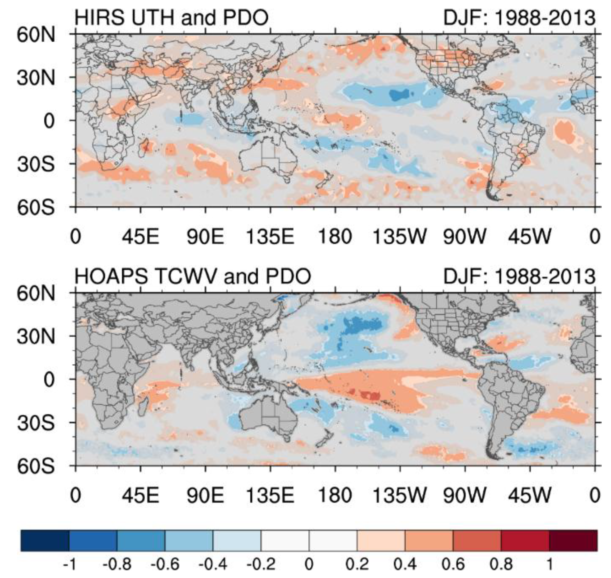
The correlations between water vapor datasets and the PDO index [56] for DJF are shown in Figure 8 for UTH (upper panel) and TCWV (lower panel). There are relatively large positive correlations extending from the western subtropics to mid-latitudes of the Pacific Ocean in the UTH field. Positive UTH correlations are also found in the central equatorial Pacific. There is a negative correlation area in the eastern Pacific near 20°N, where water vapor is likely reduced by the stronger subsidence during the positive phase of PDO, and thus negative correlations are enhanced. Following the PDO index, this area more likely experiences weakened subsidence during the negative phase of PDO. For the TCWV correlation field, though, the northern mid-latitude positive correlations are located in the eastern Pacific. Positive correlations are more prominent along the equatorial Pacific. The similarity in the locations of negative and positive areas between Figure 7 and Figure 8 illustrates a strong linkage between PDO and ENSO events. Using observational data and the output of 19 models from the Coupled Model Intercomparison Project Phase 5 (CMIP5), Lin et al. [60] demonstrated that El Niño is 300 percent more frequent than La Niña in positive PDO phases, and 58 percent less frequent in negative PDO phases.

3.4. Lag Correlations

Though both UTH and TCWV have high correlations with climate indices, the phases of correlations with indices can be lagging. Lag correlation analyses of various atmospheric and hydrological variables with SST indices have been extensively studied and often used for forecasts [61,62,63]. 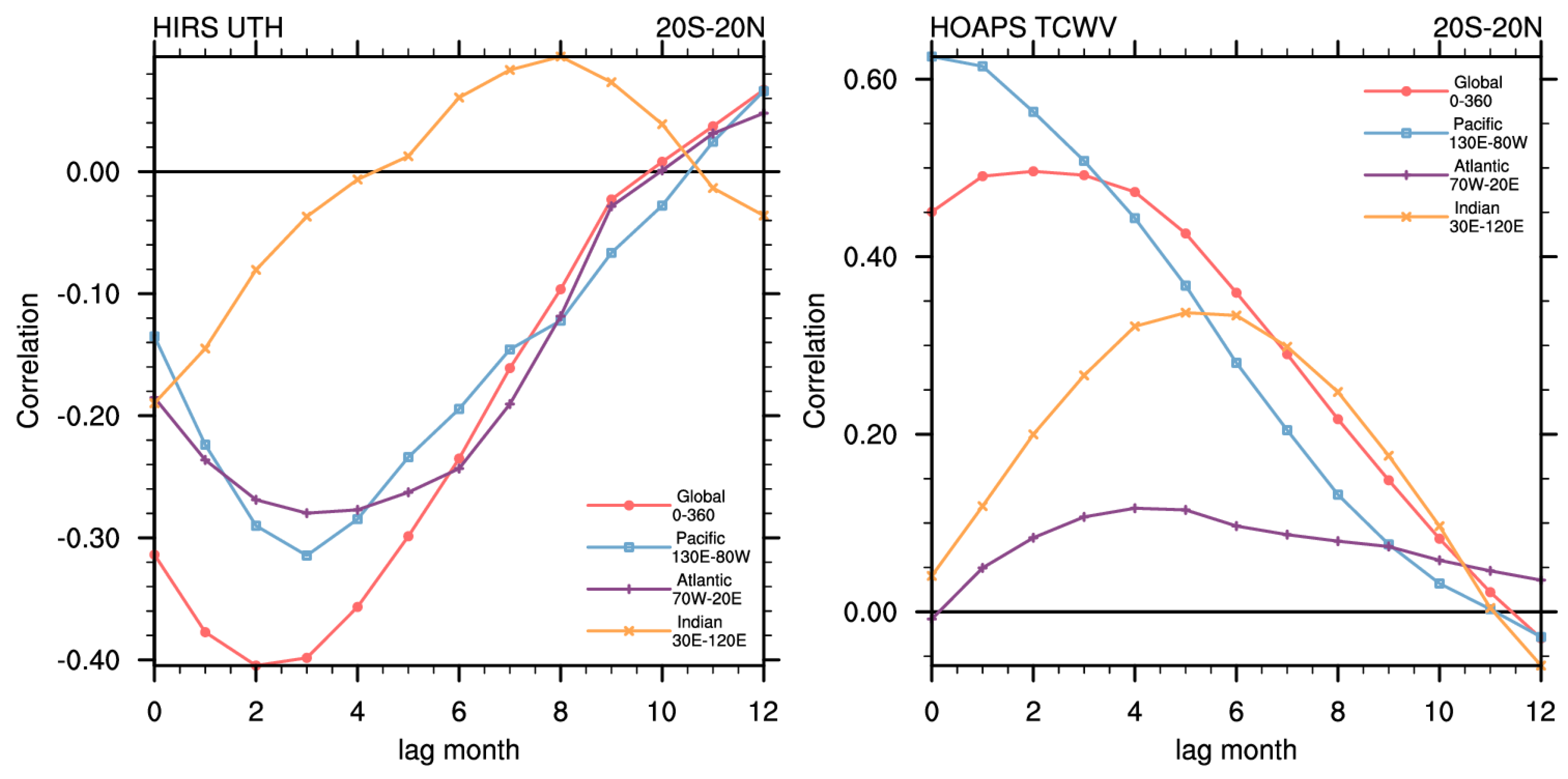The correlations present additional details of teleconnections in different regions as an integral part of the global system, through interactions of atmospheric systems such as large-scale transport of air masses with various frequencies of waves [64,65] and other systems. The lag correlation analyses of UTH and TCWV with the Niño 3.4 index over the zonal mean 20°S–20°N and over three tropical oceans within 20°S–20°N are shown in Figure 9. Averaged over 20°S–20°N, correlations for TCWV with the Niño 3.4 index are mostly positive over all regions considered, including around-the-globe and the three oceans analyzed. However, because of large cancelling effects and negative anomalies being more dominant during El Niño events in UTH between the equatorial and subtropical latitudes, UTH correlations are mostly negative for around-the-globe and for the Pacific and Atlantic Oceans. Only the Indian Ocean shows a peak of positive lag at eight months. Over the Pacific, the TCWV correlation does not have a lag from the Niño 3.4 index, while for UTH, there is a negative lag of three months.

When the analysis is focused on the equatorial belt 5°S–5°N (Figure 10), with the removal of subtropical effects, the Pacific UTH correlation changes sign to having a positive correlation with the Niño 3.4 index. The average of the around-the-globe correlation for UTH is very small due to approximately equal amount of positive and negative correlations cancelling each other out. The correlations for the Atlantic and Indian Oceans are negative through ENSO teleconnection effects. For the TCWV, the correlation patterns over 5°S–5°N are relatively similar to those over 20°S–20°N, and the teleconnection effect on the Atlantic and Indian Oceans remains positive. Based on Figure 7, TCWV is much more sensitive to the ascending branch over the equatorial Pacific, to the point where it would drown out the subtropical signals in a 20°S–20°N average. UTH is more balanced, but tilted a bit towards the subtropical signals, thus adding more compensating effects into the average. These differences arise from the different characteristics of the two water vapor datasets. The moisture on the equator is largely bottom-up, driven by surface fluxes from the SST anomalies, so they show up more strongly in TCWV. Meanwhile, the subtropical signals are driven more by compensating subsidence in the subtropics, which are more top-down and show up more in UTH.

4. Conclusions

As part of the GEWEX water vapor assessment activities, this study examines the temporal and spatial patterns of UTH and TCWV during major El Niño events. Both UTH and TCWV exhibit significant variations in relation to El Niño conditions. However, the phase of the UTH variation in a tropical-wide zonal mean can be in the opposite mode from that of the TCWV. The variation of UTH is more dependent on the locations of atmospheric circulations, and there are larger areas of drying than those of moistening in the upper troposphere during a major El Niño event in the tropics (20°S–20°N). During such an event, the TCWV increases significantly over large areas of the tropics, while the corresponding decrease of TCWV in other, smaller areas of the tropics usually occurs in smaller magnitudes. In the meantime, the UTH variation pattern is very different. Decreases of UTH are observed over large areas of the tropics, corresponding to both the weakened ascending branch of the general circulation in the western Pacific and the enhanced descending branches along the Pacific subtropics. Furthermore, the magnitude of negative UTH anomalies is equivalent or larger than the magnitude of positive anomalies. The most significant increase of UTH is found primarily over a narrow belt of the equatorial central–eastern Pacific. This results in opposite phases between UTH and TCWV in the time series when a tropical zonal average is taken. However, when only the equatorial central–eastern Pacific region is considered for UTH, the temporal variation phase of UTH is consistent with that of TCWV.

The study also shows that the variations of UTH and TCWV are closely correlated with major climate indices such as Niño 3.4 and PDO. Both UTH and TCWV are able to capture major sources of climate variability. However, differences are shown between the UTH and TCWV correlation patterns with the climate indices. Large values of correlations in the TCWV fields are more confined to the Pacific Ocean. The differences in dependencies of atmospheric general circulations for UTH and TCWV also result in significantly different lag correlation patterns with the Niño 3.4 index between UTH and TCWV. Over the tropical oceans, the TCWV fields show almost all positive correlations of various lag times. The TCWV over the Pacific has no lag with the Niño 3.4 index. However, the UTH fields have negative correlations except for the Indian Ocean when the average is taken from 20°S–20°N. The Pacific UTH correlation becomes positive and does not lag with the Niño 3.4 index only when the analysis is focused on the equatorial Pacific.