Lead Detection in Polar Oceans—A Comparison of Different Classification Methods for Cryosat-2 SAR Data

Abstract

In polar regions, sea-ice hinders the precise observation of Sea Surface Heights (SSH) by satellite altimetry. In order to derive reliable heights for the openings within the ice, two steps have to be fulfilled: (1) the correct identification of water (e.g., in leads or polynias), a process known as lead classification; and (2) dedicated retracking algorithms to extract the ranges from the radar echoes. This study focuses on the first point and aims at identifying the best available lead classification method for Cryosat-2 SAR data. Four different altimeter lead classification methods are compared and assessed with respect to very high resolution airborne imagery. These methods are the maximum power classifier; multi-parameter classification method primarily based on pulse peakiness; multi-observation analysis of stack peakiness; and an unsupervised classification method. The unsupervised classification method with 25 clusters consistently performs best with an overall accuracy of 97%. Furthermore, this method does not require any knowledge of specific ice characteristics within the study area and is therefore the recommended lead detection algorithm for Cryosat-2 SAR in polar oceans.

1. Introduction

Satellite altimeter missions have been providing precise measurements of the Sea Surface Height (SSH) on a nearly global scale for more than 25 years. This data set has significantly improved our understanding of the sea level dynamics. However, in the polar regions, the altimetry measurements are contaminated by the sea-ice resulting in a degradation in the precision or even usefulness of the results. Radar altimeter observations in the vicinity of sea-ice typically result in an over-estimation of SSH [1]. Knowledge of the locations of openings within the sea-ice, known as leads, can help improve the SSH estimation and the understanding of the global climate. For instance, the SSH derived through leads is assumed to be the instantaneous ocean elevation which can be used to estimate the sea-ice freeboard [2,3]. Therefore, it is clear to see that a reliable SSH is essential for the estimation of the freeboard thickness. Freeboard estimates can be negatively biased when an unreliable lead detection is imposed and the SSH precision is degraded by ice samples detected as leads [1]. Accordingly, the reliable identification of leads is an essential criteria for precisely monitoring the Arctic ice volume decrease, as well as for Arctic sea level change studies.

Indications to the usefulness of satellite altimetry for finding open water within sea-ice were provided as early as 1980 by Dwyer and Godin [4]. They were able to determine the sea-ice boundary using GEOS-3 satellite altimetry data with the knowledge that within sea-ice regions, the altimetry backscattering properties are in stark contrast to that of open water. The altimeter returned signal, known as a waveform, provides this backscattering information. Leads are known to produce high power and single peak specular returns in altimeter waveforms. This is because leads typically have a smooth (relative to the radar wavelength) surface as they generally are absent of any wave field, meaning a large percentage of the radiated energy is reflected back towards the antenna of the satellite [4,5].

To date, many methods to find leads based on altimeter observations have been implemented. Laxon [5] developed a parameter based on the maximum power of ERS satellite altimeter waveforms, pulse peakiness, which could be used for charting the open water areas within the Arctic regions. Connor et al. [6] also used the pulse peakiness parameter with Envisat data to find leads in order to make estimates of the sea-ice freeboard. Röhrs and Kaleschke [7] used a maximum power threshold on Cryosat-2 (CS-2) SAR altimeter waveforms to identify leads. Zygmuntowska et al. [8] developed a supervised classification method based on Bayesian classification [9] applied to ASIRAS (airborne version of the SIRAL instrument on-board CS-2) waveform shape parameters. Passaro et al. [10] developed a parameter based on the stack waveforms of CS-2 known as the stack peakiness. This parameter also considers multiple consecutive observations in an attempt to isolate a lead at the nadir position. Müller et al. [11] developed an unsupervised classification method based on K-medoids partitional clustering [12] of model waveform features and classification of observation data relative to the model using K-nearest neighbor (KNN) classification [13]. Shen et al. [14] aimed to find an optimal classifier–feature assembly for sea-ice classification. They tested a number of waveform feature statistical methods with different combinations of waveform features. Just recently, Lee et al. [15] proposed a promising new method for detecting leads using CS-2 waveforms. Their method is based on a waveform mixture analysis, which assumes that each footprint of the waveform is a linear combination of leads and various types of sea-ice.

Most of the above mentioned studies include a validation of the presented results. However, since they are based on different input data, different ground truth data sets and different accuracy metrics, they are not directly comparable. To overcome this deficiency and to recommend the best classification method for further applications is the motivation of this investigation.

Within this study, four lead classification methods are tested for CS-2 SAR data and evaluated using high resolution imagery acquired during CS-2 dedicated underflights. The aim is to find the best existing CS-2 SAR altimeter lead classification algorithm that provides low false classification. The four classification methods under investigation are (1) the waveform maximum power as introduced, e.g., by Röhrs and Kaleschke [7]; (2) the multi-parameter classification method primarily based on pulse peakiness developed by Ricker et al. [16]; (3) a method based on the stack peakiness presented by Passaro et al. [10]; and (4) the unsupervised classification method published by Müller et al. [11].

This is the first study that compares different classification approaches using exactly the same input data and the same very high resolution (<1 m) ground truth. Previous studies have used space-based evaluation techniques that have suffered from a relatively low resolution, meaning that small scale leads are not observed by the ground truth and, therefore, they bias the classification results. Furthermore, observations with time differences of multiple hours have been utilized, also distorting the results. In contrast, here, almost time coincident ground truth data is used.

This paper is structured as follows. Section 2 describes the CS-2 altimeter SAR data sets and some of their processing parameters as well as the ground truth image data sets. A brief description of each employed lead classification method together with an overview of the threshold optimization technique is given in Section 3. A quantitative comparison of all lead classification methods relative to the ground truth combined with a discussion of the results is provided in Section 4. Finally, the conclusion summarizes the results and provides the reader with a recommendation for the “best” lead classification method based on the available data.

2. Data Sets and Study Areas

This section will discuss the CS-2 data sets, the ground truth used for evaluating the classification methods, and the corresponding study areas.

2.1. CryoSat-2 Data

The CS-2 mission is the first satellite altimeter utilizing the so-called Delay-Doppler or SAR concept in some geographical regions, among them large parts of the Polar Oceans (depending on a changing mode mask [17]). The basic idea behind the SAR principle is that the antenna size is synthetically increased (in the along-track direction) allowing to create a coherence of the emitted pulses [18]. SAR altimeters are described as being beam-limited in the along-track direction while being pulse-limited in the across-track direction. Along-track processing improves the respective resolution and furthermore, the multi-looked processing greatly improves the signal-to-noise ratio [19]. While the footprint of CS-2 yields about 300 m in the along-track direction, in the cross-track direction up to 15 km are covered by the signal [20].

For this study, in addition to the averaged multi-looked waveforms, full stack data is needed. ESA grants access to an online service called Grid Processing On-Demand (GPOD), which provides the full stack (L1B-S) for the CS-2 mission. The CS-2 data sets used within this study (mainly multi-looked waveforms and derived parameters) are all taken from the SAR Versatile Altimetric Toolkit for Ocean Research & Exploitation (SARvatore) GPOD service (see acknowledgments). The GPOD service allows for free and easy access to two main data products, namely ESA Baseline C L1B-S and L2 data [21]. The online service allows for tailored processing of each product. Dinardo [22] has described in detail the processing steps for L1B data. For the present study, a Hamming window is applied before the along-track Fast Fourier Transform in an attempt to stop signals coming from leads that are outside the synthetic along-track 3 dB beam-width (main-lobe), as recommended by Passaro et al. [10].

2.2. Ground Truth Data

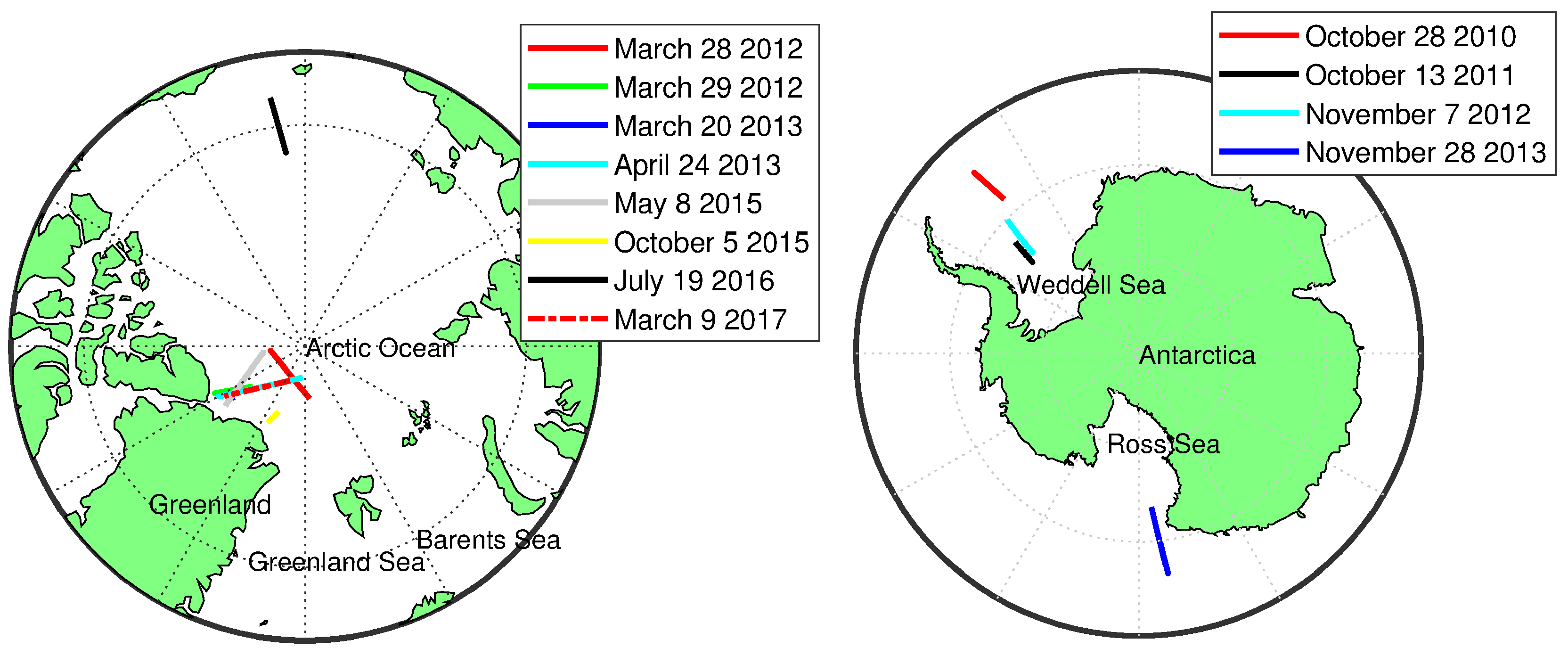
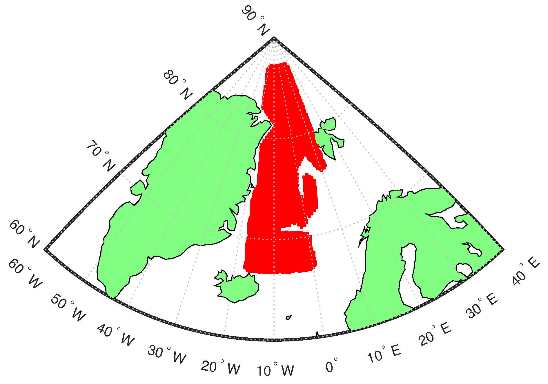
For evaluating lead classification results, the contemporaneity between altimetry measurements and ground truth observations is of great importance in order to exclude any differences due to sea-ice drifts. The NASA Operation IceBridge (OIB) mission [23] includes several CS-2 underflights, following the CS-2 groundtracks in Arctic and Antarctica with very short time discrepancy in overpassing [24]. Moreover, airborne sensors acquire cloud-free images with a very high resolution.

The ground truth validation data used within this study is the Operation IceBridge Digital Mapping System (DMS) L1B geolocated and orthorectified images [25]. These images are panchromatic and provide a very high resolution, making them an ideal choice for lead detection. The pixel resolution for a flight height of 450 m is about 10 cm × 10 cm, resulting in an image size of approximately 775 m × 690 m. Within this study, the images are resampled into 1 m resolution in order to reduce the computational costs. This resolution is deemed sufficient for detecting even small leads, especially since the CS-2 resolution is significant lower (see Section 2.1).

2.3. Flight Lines

In order to ensure a reliable validation, CS-2 observations are selected on tracks that are simultaneous and almost time-coincident with the airborne underflights from the NASA Operation IceBridge mission. In total, 12 data sets were found defining the validation data set from polar regions within this study (eight on the northern hemisphere, four on the southern hemisphere). Figure 1 illustrates the locations of these data sets for the Arctic and Antarctic regions, respectively. The majority of the data sets are taken from the spring season.

Airborne images that were acquired later than 90 min after the satellite overpass and earlier than 90 min before the satellite overpass are discarded from the analysis. This threshold is chosen as an optimum balance between having sufficient data to perform this study and preventing lead positional errors due to the sea-ice motion which may bias the statistical results. Additionally, adapting the methodology from Ricker et al. [16] to coarsely discriminate between open ocean and sea-ice, only those data observed with a sea-ice concentration greater than 70% are used, since the theoretical basis for lead detection may no longer hold in low sea-ice concentration areas. The sea-ice concentration values used in this study are the interpolated sea-ice concentration values available from the Ocean and Sea-Ice Satellite Application Facility (OSI SAF) (see acknowledgments).

3. Methodology

This section gives an overview of the employed four lead classification methods, whose performances will be compared within this paper. Moreover, the methods used for ground truth image classification and for optimal threshold definition will be described.

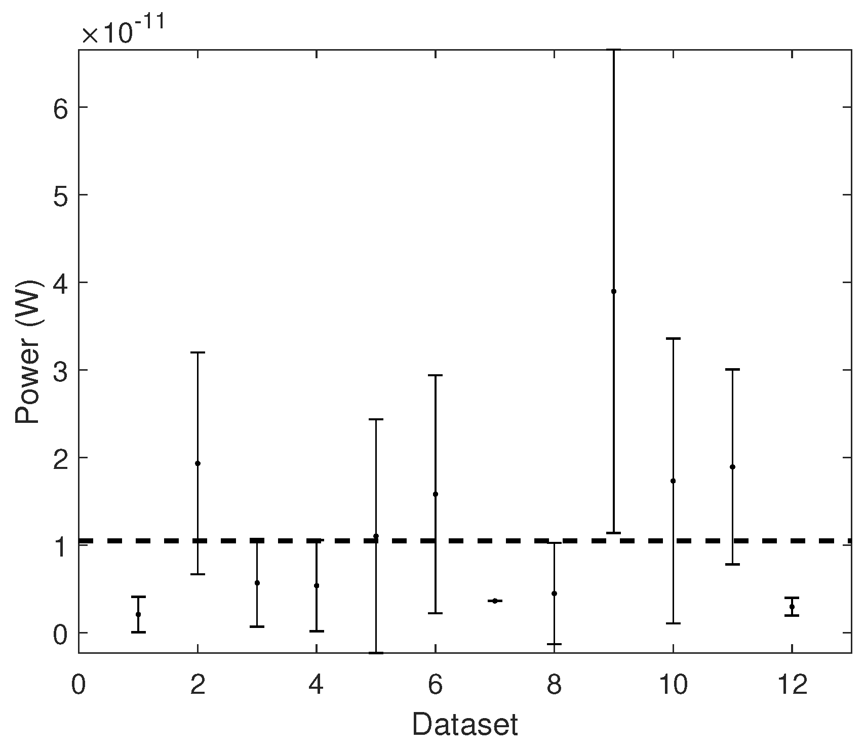
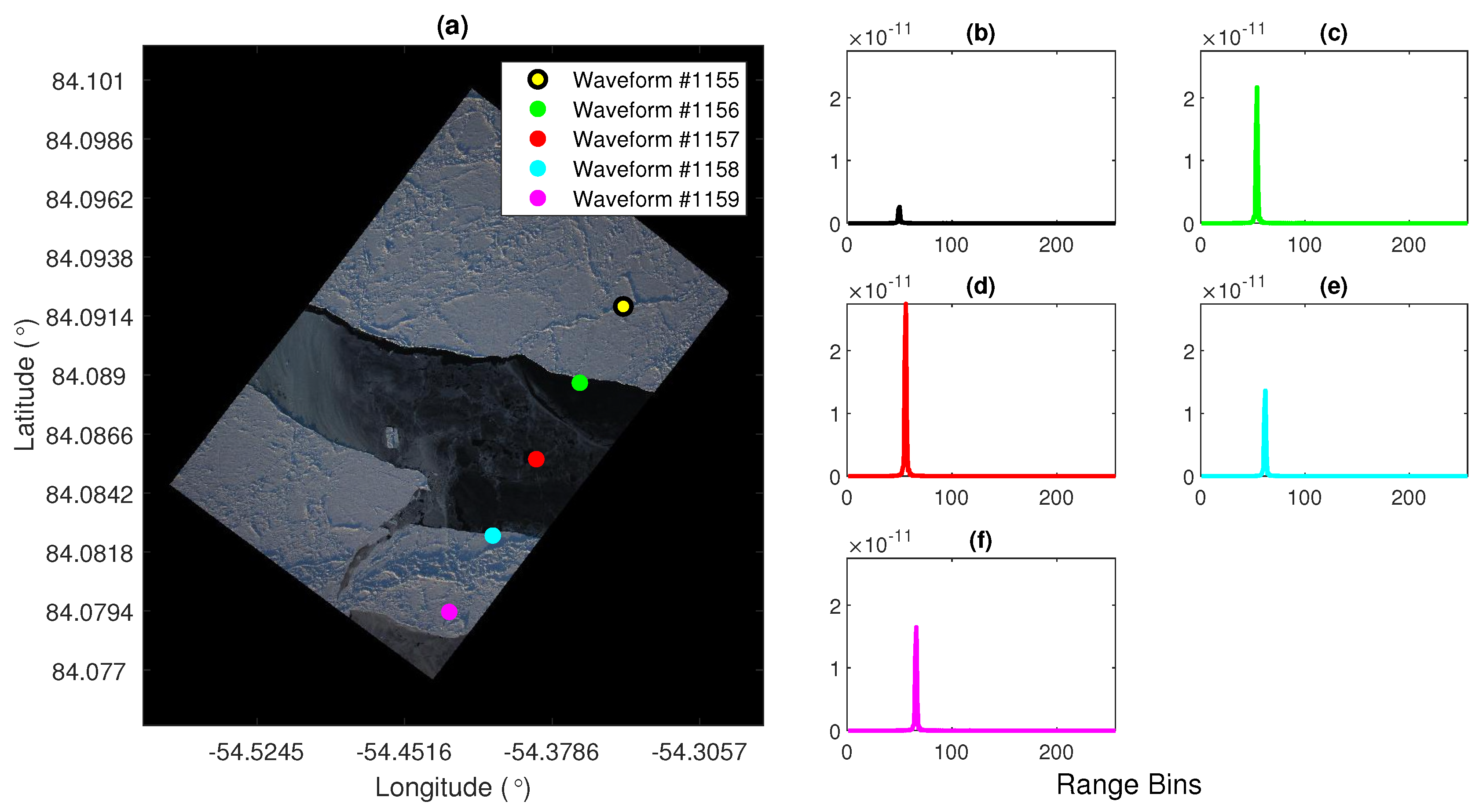
3.1. Maximum Power Classifier (MAX)

The maximum power classifier [7] has the simplest implementation of all the classification methods used within this study. It relies on the application of a threshold to the maximum power of multi-looked altimetry waveforms. If the maximum power is above the threshold, then the corresponding observation is classified as a lead. In a similar previous study, Wernecke and Kaleschke [1] found the maximum power classifier to be the best lead classification method with their ground truth validation data—MODIS satellite imagery. Although the maximum power classifier has an easy implementation, it does require knowledge of the study area in order to correctly define the threshold, which is usually not assured. Moreover, the maximum waveform power—and thus the correct threshold—is known to vary substantially across different regions and seasons [10].

3.2. Multi-Parameter Classification Method (MULTI)

The second lead classification method used in this study is the one proposed by Ricker et al. [16], which uses six parameters in order to discriminate a lead observation from one over sea-ice. The parameters are:

• Pulse Peakiness (PP): Defined as the ratio of the waveform maximum power to the accumulated power and also in this case scaled by the number of range bins. Larger values are indicative of the presence of a lead within the altimeter footprint.
• Stack Kurtosis (K): An additional measure of the peakiness of the range integrated stack power [26]. A high value suggests that the distribution is prone to an outlier, e.g., caused by the presence of a lead within the altimeter footprint.
• Stack Standard Deviation (SSD): This value provides information to the variation of surface backscattering power with incidence angle [26]. Therefore, small values of SSD are used as an indicator for the presence of leads.
• Modified PP (two parameters $P{P}_l$ and $P{P}_r$ to consider the bins “left” and “right” of the maximum power bin): This is meant to disregard lead observations which are not at nadir. The assumption here is that off-nadir lead reflections do no show as specular a reflection as an observation at nadir.
• Sea-ice concentration: This is used as a coarse discrimination between ocean and ice areas. Only observations in areas with significant sea-ice concentration (>70%) are allowed as leads in case all other conditions are met.

The MULTI method also requires the definition of thresholds for all parameters, which are used to discriminate lead observations from sea-ice observations. Furthermore, the correct setup of the thresholds requires knowledge of the sea-ice characteristics and are usually not transferable between different regions.

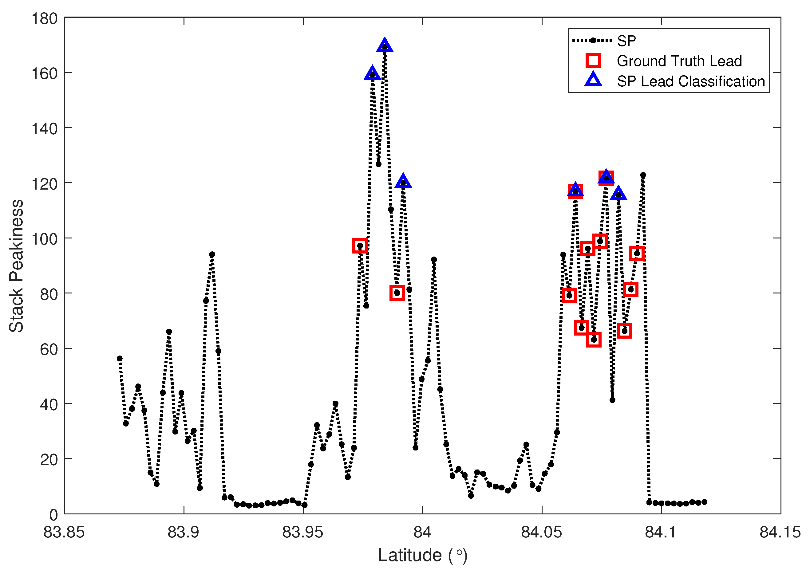
3.3. Stack Peakiness Classifier (STACK)

The stack kurtosis and SSD can be used to classify a waveform that might contain a lead, but they are independently insufficient in isolating a nadir return from a stack of waveforms which has observed a lead backscatter. This was the motivation of Passaro et al. [10] to develop the Stack Peakiness (SP) parameter that is defined using the Range Integrated Power (RIP) normalized against its maximum value. For CS-2 Baseline C, the SP parameter must be computed using the stack data available from the GPOD website, as it is not available in the official Baseline C L2 data product. However, it is included in the Baseline D L2 data.

The assumption behind the algorithm is that larger local maxima in SP are likely to be evoked by a lead at nadir. Therefore, a multi-observation analysis occurs before a lead classification is made, which considers the current, forward and aft observations. The forward and aft observations must be above the median SP ($S{P}_{median}$) plus Median Absolute Deviation MAD ($S{P}_{MAD}$) of all CS-2 tracks within this study for the current observation to be considered a lead. This is done in an attempt to reduce false lead observations as a lead within the altimeter footprint influences the SP value even when not at nadir. The current observation must also be above a predefined minimum threshold ($S{P}_{minlead}$) in order for it to be classified as a lead.

The SP strategy developed in Passaro et al. [10] had the objective of isolating one single return in each lead, without distinguishing other reflecting surfaces. In contrast, within this study all observations above a lead are considered as part of the statistical analysis. This therefore increases the percentage of points considered as erroneous ice detections in this study (see Section 4).

The performance of this classification method depends on the correct threshold definition as much as the two previous methods. Section 3.5 will handle the threshold optimization.

3.4. Unsupervised Classifier (UNSU)

The unsupervised classification method developed by Müller et al. [11] is believed to be the first attempt using this method applied to satellite altimetry over sea-ice areas. There are many different approaches to unsupervised learning including clustering (e.g., K-means, K-medoids [27]), latent variable models (e.g., Hidden Markov Models [28]) and others. Müller et al. [11] employed the clustering K-medoids algorithm for their unsupervised classification on pulse-limited altimetry waveforms (Envisat and SARAL). In this study, the unsupervised classification method is tested for the first time with SAR altimeter data.

The first step in the unsupervised classification process is to cluster or group model data applying the K-medoids algorithm. The six waveform features defined by Müller et al. [11] are also used for the clustering in this study, with minor changes in some computation parameters:

• Waveform maximum (Wm): As described in Section 3.1, the maximum power can be used to characterize the surface below the satellite altimeter.
• Trailing edge decline (Ted): The Ted is a characterization of the trailing edge of the waveform, i.e., from the maximum power range bin to the last range bin, by means of a fitting to a power series model. A rapid decay (low value) would be associated to the typical waveform shape of a lead.
• Waveform noise (Wn): In the context presented here, the Wn represents the MAD of the residuals to the fitting of the power series model. Very small values for specular lead type returns are expected.
• Waveform width (Ww): The amount of range bins with their power greater than 1% of the waveform maximum is used to determine the waveform width. A small waveform width is expected in the presence of a lead.
• Leading edge slope (Les): The first waveform bin containing more than 12.5% of the waveform maximum power subtracted from the maximum power bin provides relative information regarding the Les. Again, low values are indicative of a lead surface.
• Trailing edge slope (Tes): Conversely, the Tes is obtained by a subtraction of the maximum waveform power bin from the last bin position containing more than 12.5% of the waveform maximum power. The characteristics of the Tes is similar to the Les for single peak waveforms, but it can also be used to identify strong multiple peaks.

The features produce varying orders of magnitudes, which causes biased weighting within the K-medoids algorithm. Therefore, before used for clustering, all features are reduced using the standard score (sometimes referred to as z-score) to give more reliable clustering results [29].

In order to have a model that is representative of as many waveform types as possible, a large collection of waveforms is required from the CS-2 mission. This has to include waveforms from sea-ice, leads and ocean surfaces. The maximal extent of the Arctic sea-ice is in March [30] and therefore, the beginning of the melt-season (April/May) is assumed as the most likely period to cover as many sea-ice types as possible. Figure 2 shows the location of the model data taken for this study from the Greenland Sea. The data used corresponds to when CS-2 was operating in SAR mode during the time period of April through to May 2015, corresponding to 361,977 model waveforms.

To initialize the K-medoids algorithm, the number of clusters k needs to be decided. The value for k should be larger than the final amount of surface classifications, i.e., $k>3$ (lead, sea-ice and ocean). Müller et al. [11] used $k=30$ which was empirically derived by means of visual analysis of the resulting clusters and sums of distances. Within this study, a test of seven cluster numbers is performed ranging from $k=5$ to $k=35$ in steps of 5.

After the K-medoids algorithm has finished, the clusters have to be classified manually to one of the surface types. The final step is then to classify observation data relative to the classified cluster model. This is done using K-Nearest Neighbor (KNN) classification. The KNN size must also be chosen and this is done using a 10-fold cross-validation method as described in detail in Müller et al. [11].

3.5. Threshold Optimization

Three of the four classification methods under investigation (namely MAX, MULTI, and STACK) depend on one or more predefined thresholds that can be determined using a reliable ground truth. Wernecke and Kaleschke [1] developed an optimization technique, which is also applied here. It minimizes a cost function to derive the threshold value $\mathsf{\Theta }$

$$\mathrm{cost}\left(\mathsf{\Theta }\right)=w\times \mathrm{False}\mathrm{Ice}\left(\mathsf{\Theta }\right)+\mathrm{False}\mathrm{Lead}\left(\mathsf{\Theta }\right)$$

(1)

where w is a weighting defining how the false classifications are minimized. “False Ice” are observations classified as ice but are actually lead samples and “False Leads” are observations classified as leads but are actually ice samples. For small values of w (i.e., <1) False Lead observations are primarily reduced and for $w=1$, the total false classifications are minimized. The ground truth is used to randomly separate the data into a training (50%) and testing (50%) subset with an equal number of sea-ice and lead samples within each subset. $\mathsf{\Theta }$ is derived from the training subset by testing all potential threshold values as initial guesses to the Nelder and Mead [31] minimization algorithm. The random sub-sampling is repeated 200 times in order to find the global minimum of the cost function and to have an estimation of the spread of performance on each testing subset. This is done for different values of w.

For MULTI, only the PP and modified PP parameters thresholds are derived using this optimization. This is done in an attempt to reduce computation time. The sea-ice concentration value does not depend on the satellite altimeter so the threshold of 70% remains. The thresholds of 40 and 4 from Ricker et al. [16] for K and SSD respectively also remain as it was found that the vast majority of lead observations fell inside these thresholds.

For STACK, the $S{P}_{median}$ and $S{P}_{MAD}$ found through the ground tracks used in this study resulted in $S{P}_{median}=9.76$ and $S{P}_{MAD}=6.33$, meaning a slightly lower sum compared to Passaro et al. [10]. For this reason, it was decided to use the values from the literature. When developing the $S{P}_{minlead}$, due to the random sampling of the data, the multi-observation analysis was not conducted for the threshold optimization.

The optimized threshold values and their corresponding weight value are given in

Table 1. Optimized thresholds and their corresponding weight.

w	Max. Power	$\mathit{PP}$	${\mathit{PP}}_{\mathit{l}}$	${\mathit{PP}}_{\mathit{r}}$	SP
0.5	$4.356\times {10}^{-11}$ W	120.75	175.08	30.84	345.02
1	$2.714\times {10}^{-11}$ W	116.18	152.58	158.11	300.43
2	$1.892\times {10}^{-11}$ W	99.93	63.25	145.29	156.61
3	$1.051\times {10}^{-11}$ W	99.67	63.38	124.28	102.86
4	$4.513\times {10}^{-12}$ W	96.71	66.05	69.28	91.28
5	$4.958\times {10}^{-12}$ W	97.01	63.92	51.59	78.61
6	$3.609\times {10}^{-12}$ W	97.03	64.15	50.89	73.47
7	$2.219\times {10}^{-12}$ W	97.00	62.25	56.19	71.14
8	$1.654\times {10}^{-12}$ W	97.15	53.80	51.43	70.41
9	$1.399\times {10}^{-12}$ W	90.18	63.20	53.98	70.41
10	$1.359\times {10}^{-12}$ W	80.47	57.32	30.40	54.03

. All of them are used to generate different classification results that are shown and discussed in Section 4.

3.6. Ground Truth Image Classification

In order to be able to compare and validate the different altimeter lead classification methods, a reliable ground truth image classification must be used. In optical images, such as the ones from IceBridge used here, leads are known to have typically dark optical features that translates to low image pixel intensities. Lead attributes can be dynamic due to different types of thin ice within the lead itself, formed by rapid ice growth due to the cold polar temperatures. Additionally, leads with thin ice may even be covered by snow and frost flowers [32].

The ground truth data for this study is set up applying the automatic Sea-Ice Lead Detection Algorithm using Minimum Signal (SILDAMS) developed by Onana et al. [33], which has been shown to give favorable results using NASA Operation IceBridge image data. The SILDAMS algorithm is based on an affine time-frequency distribution analysis which uses the minimum signal transform in order to perform a localization around low frequencies. The minimum signal is given by

$$S_{min}^z\left(f\right)=f^{2\pi z}{e}^{-2\pi zf}$$

(2)

where f represents the frequency or image pixel intensities and z is a positive parameter for adjusting the spectral width (bandwidth). With a careful selection of the z parameter, it is possible to highlight features of interest from the image, such as leads. The bandwidth parameter is defined as $z=0.001$, since this value has been shown by Onana et al. [33] to provide good results for images acquired in clear conditions with daylight. As one of the OIB data sets (taken on 28 October 2010) was acquired in ever decreasing lighting conditions. From a visual analysis of the images, it was decided to change z according to the lighting conditions from $z=0.003$ for the first 450 images, to $z=0.005$ (from 451 to 1035), $z=0.006$ (from 1036 to 1103), and $z=0.015$ (for the remainder of the images).

The last step in the image classification is to apply a threshold to the minimum signal transformation of the image. Within this study, only a binary classification is used between sea-ice and lead/open water. In accordance with Onana et al. [33], a threshold of $0.3$ is used for water detection (smaller values = sea ice; larger values = lead). This results in a binary map for each image with a one indicating a lead pixel and a zero indicating a sea-ice pixel. Nearest-neighbor interpolation is then used to associate the binary classification to the CS-2 surface sample ground track.

All images are assumed to be cloud-free since a manual inspection of completeness of laser measurements from the laser-based Airborne Topographic Mapper (ATM) revealed almost no missing values.

Onana et al. [33] specify the lead detection capability of SILDAMS to be 99%. The manual inspection of the ground truth data set established in the present study shows that all open water areas are correctly flagged without any false detections. However, the distinction between open water and thin ice was only correct at about 90%. For this reason, the open water class also contains thin ice—which is uncritical for altimetry waveform classification which can also not differentiate very thin ice from leads [6].

4. Results and Discussion

In order to be able to assess each altimeter classification method, they must be compared with the same ground truth, which is derived from the image classification described earlier. This section provides and discusses the results of the ground truth evaluation and comparison between each altimeter classification method. In total, there are 14,231 satellite observations from all the data sets, and of these, 365 observations (i.e., about 2.5%) are defined as leads (including leads with thin ice) according to the ground truth.

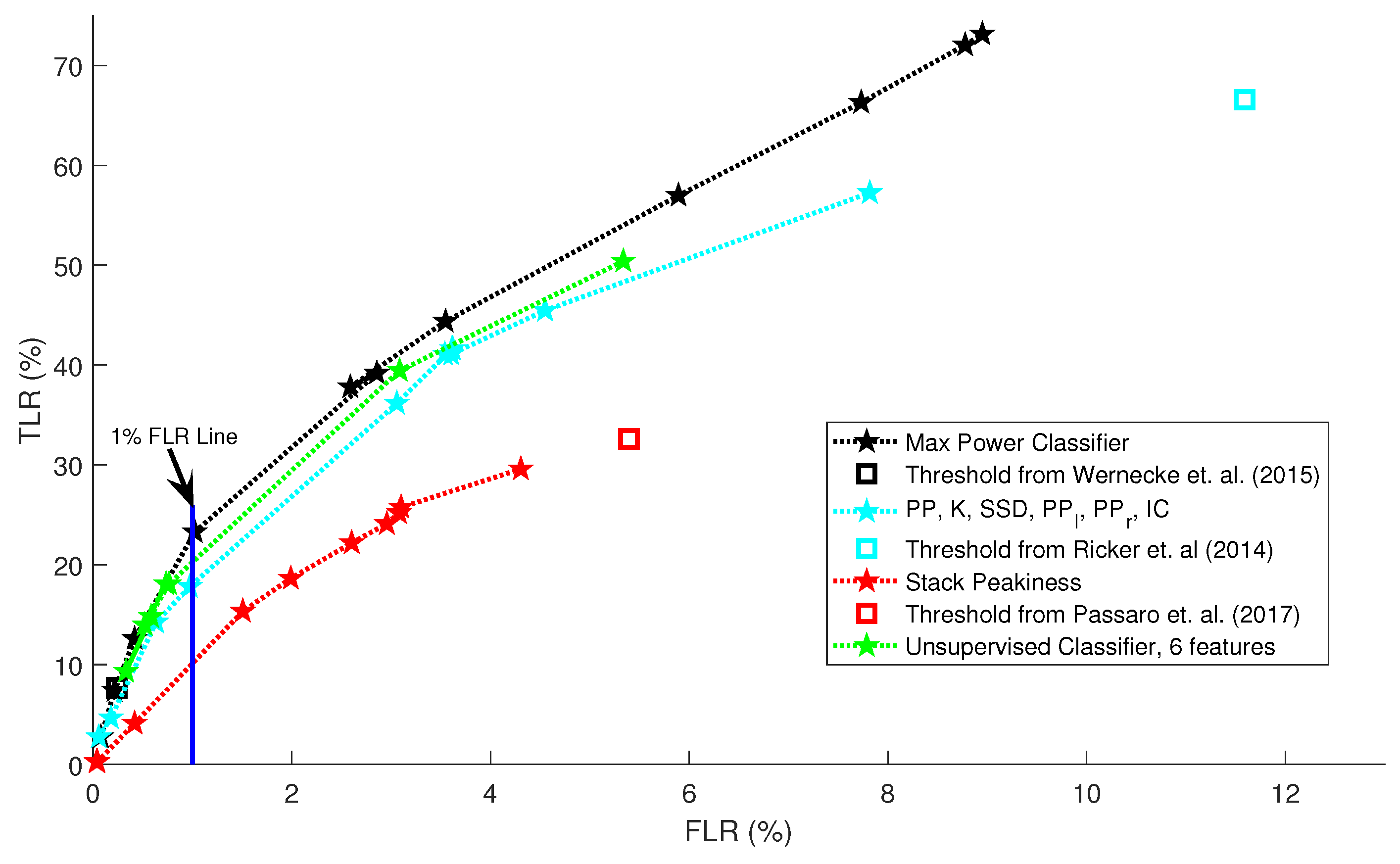
4.1. Quantitative Comparison between Altimeter Classification and Ground Truth

A Receiver Operating Characteristics (ROC) graph [34] is used to visualize the performance of the different classifiers (see Figure 3). It shows the change in performance of the different altimeter classification methods relative to the ground truth depending on different thresholds. Two criteria are computed for the evaluation: the True Lead Rate (TLR), which is the percentage of leads classified by the altimeter classification and confirmed by the ground truth classification (see Equation (3)) and the False Lead Rate (FLR), which is the percentage of altimeter lead classifications that are classified as sea-ice by the ground truth to the total sea-ice ground truth samples (see Equation (4)).

$$\mathrm{TLR}=\frac{\mathrm{True}\mathrm{Lead}}{\mathrm{True}\mathrm{Lead}+\mathrm{False}\mathrm{Ice}}$$

(3)

$$\mathrm{FLR}=\frac{\mathrm{False}\mathrm{Lead}}{\mathrm{False}\mathrm{Lead}+\mathrm{True}\mathrm{Ice}}$$

(4)

True Lead is the number of observations classified as lead confirmed by the ground truth. False Ice is classified as ice observations but are lead samples according to the ground truth. False Lead observations are classified as a lead but are ice samples according to the ground truth. True Ice are observations classified as ice samples and are confirmed by the ground truth.

The aim of the ROC graphs in Figure 3 is threefold: It helps to find the best threshold for each classification method, it can be used for an inter-comparison of the methods, and it provides a quantitative performance measure for all classifiers. In general, with an increasing weight w (as defined in Equation (1)) there is an increase in the TLR and also the FLR for all classifiers with a higher rate of increase in the TLR. However, this behavior is not linear, and there seems to be a maximum TLR reachable for each method. When further increasing the weight (i.e., lowering the threshold) this only results in a larger FLR. This effect was already shown by Wernecke and Kaleschke [1].

Simply from looking at Figure 3, it is not immediately clear what is the best threshold/number of clusters to use. This strongly depends on the application, i.e., on the acceptable FLR. In case it is important to reach a very low FLR, a conservative threshold (small weight) should be used. This comes at the cost of identified leads. However, if the application requires as many leads as possible, one should use a higher w. All three classifiers reach TLR between 30% and 55% when FLR of 5% are acceptable. From Figure 3, it seems that the MAX classification method performs best for the majority of weights compared to all other classification methods, followed closely by UNSU and MULTI. The STACK classification method appears to be the poorest performing classifier, showing a narrow ROC curve with a small TLR/FLR ratio that is about half of that from MAX. The highest overall TLR of about 75% is achieved by MAX (with FLR of about 10%).

In order to quantify and compare the performance of the different classifiers, a fixed FLR is defined and the corresponding TLR are compared. A FLR of 1% is chosen as an optimum balance between a relatively high TLR and low number of false open water observations. For the MAX classifier, this results in a TLR at 23.05% (closest threshold $w=3$; $1.05\times {10}^{-11}$ W). The MULTI method results in a 18.09% TLR (closest threshold $w=3$; $PP=99.67$, $P{P}_l=63.38$, $P{P}_r=124.28$). The STACK gives a performance of 10.38% TLR (closest threshold $w=3$; $S{P}_{minlead}=102.86$). The above TLR values were derived by a polynomial curve fitting to the points of each threshold classifier. From all threshold based classifiers, this appears to show that the maximum power classifier is performing the best relative to the ground truth.

The UNSU classification method is independent from any threshold definition. Instead, the classification performance clearly depends on the number of clusters used within the process (see Section 3.4). It can be noted that for smaller k, there is typically a larger TLR and FLR. However, in contrast to the threshold-based methods, a continuous change in performance is not observed for a change in cluster number. This is illustrated in Figure 4; the figure shows the ROC graph for UNSU in dependence of k. The optimal cluster number depends on the size and variability of the input waveform data set. If only a small number of clusters is allowed, the number of observations per cluster (i.e., the cluster size) increases and the probability for correct classification decreases. In other words: the clustering is too coarse [35]. This is the case for $k\le 10$. If k is large enough, the results only change marginally, depending on the manual preprocessing step assigning each cluster to one surface type (lead, ice, or ocean). The cluster number with FLR closest to 1% will be chosen as the optimum for this study. This corresponds to $k=25$ and results in a 18.08% TLR and 0.73% FLR. The interpolated value at 1% FLR is 22.37% TLR.

ROC graphs are useful for analyzing the performance of classifiers relative to a ground truth, and to identify the best parameters (i.e., thresholds or number of clusters) for the respective application. However, in order to understand the overall performance of the different altimeter classifiers, different accuracy metrics must be analyzed. Producer and user accuracies are used for this purpose for both sea-ice and lead samples. While producer accuracies give an indication of the probability that a ground truth sample will be correctly classified, the user accuracy is an indication to the reliability of the classification and is defined as the ratio of the sum of correct classifications (leads and ice) to the total number of classifications [36].

Table 2. Accuracies for each classifier in (%). Values provided for FLR of about 1% ($w=3$, $k=25$). The best performance for each of the accuracy metrics is marked in bold.

	MAX	MULTI	STACK	UNSU
FLR	1.02	0.79	1.51	0.73
Overall Accuracy	97.03	96.94	96.36	97.18
Lead User Accuracy	37.44	32.50	21.13	39.29
Lead Producer Accuracy (TLR)	23.29	17.81	15.34	18.08
Ice User Accuracy	98.00	97.86	97.79	97.87
Ice Producer Accuracy	98.98	99.03	98.49	99.26

lists the overall lead and sea-ice accuracies for each altimeter classification with respect to the ground truth. The largest overall accuracy is achieved by the unsupervised classification method at 97.2%. This method also yields the best lead user accuracy and the largest ice producer accuracy. However, the lead producer accuracy scores only second behind the maximum power classifier. Even if the numbers in some of the metrics only slightly differ, it is obvious that the two methods utilizing the maximum power for the classification (UNSU and MAX) score better than the other two (MULTI and STACK). While interpreting the numbers, it should be kept in mind, that all values have been optimized to score a FLR of about 1%. Since only integer weighting factors w are used, slightly different FLR are achieved and the numbers are not fully comparable. The good performance of UNSU is even emphasized, taking the lower FLR into account.

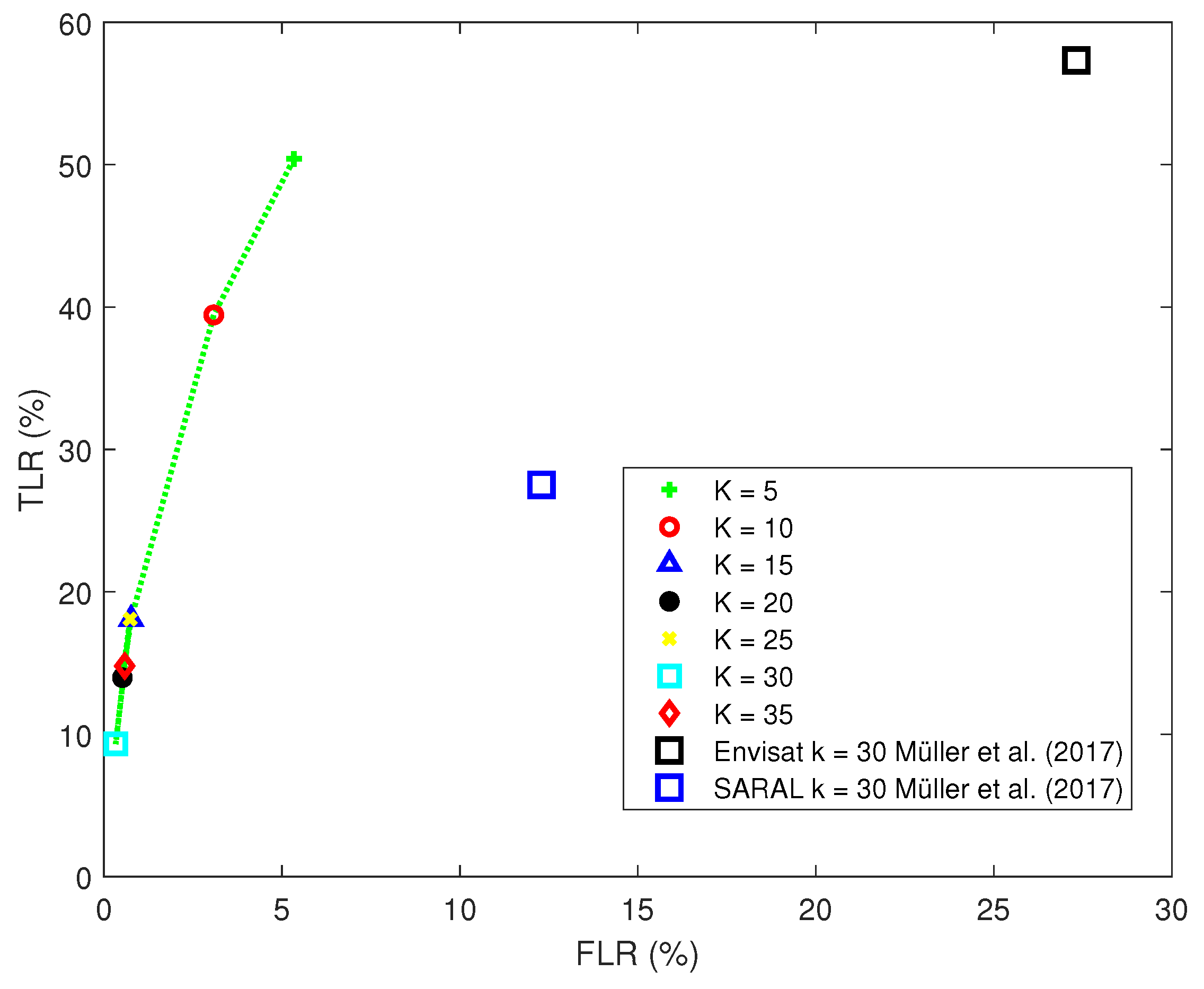
4.2. Comparison to Other Studies

The statistics presented above are not directly comparable to results from previous studies. This is mainly due to different input data sets (e.g., different missions [11] or different Cryosat-2 Baselines [1]), different thresholds used within the studies [1,10,16], and a different ground truth used for validation. Most of the older studies used ground truth data sets whose resolutions were limited to many meters (40 m to 250 m; instead of 1 m used here) and therefore, potentially, many leads have been missed. Furthermore, the time between image acquisition and satellite overpass has been limited here to 90 min, meaning there is less of a possibility of induced sea-ice drift related biases in the ground truth results.

In comparison to Passaro et al. [10], the validation approach differs significantly. Their study was focused on the detection of leads with different sizes, whereas here, the detection of altimetry returns over leads is the aim. Thus, instead of counting each lead observation separately, they considered consecutive lead observations to be the same lead. If a single observation from a lead with multiple observations was correctly classified, the overall lead was assumed to be correctly classified. This directly influences the corresponding statistics and for that reason, the results presented in this study appear poorer. However, for lead prospection, they found that the MULTI classification performed on par with the STACK when compared using the ratio of correctly classified leads to false detections.

Müller et al. [11] used exactly the same metrics to validate their results, however, a different ground truth was applied. From Figure 4 it seems that in this study a better performance can be achieved. This is presumably related to the fact that CS-2 has an improved along-track resolution with respect to Envisat and SARAL (i.e., SAR stack data compared to classical pulse-limited altimetry performs better). Though, in order to prove this, the validation of Müller et al. [11] should be repeated based on a high-resolution ground truth.

4.3. Discussion of Altimeter Classification Methods

Threshold Definition: From the previous sections it became clear that those classification methods based on the maximum waveform power perform better than the rest. However, the success of MAX strongly depends on the defined threshold. Many factors affect the backscattering power received at the altimeter antenna. This is clearly evident in Figure 5, which shows the mean and standard deviation of the maximum power at lead surfaces (at nadir) according to the ground truth for each data set used within this study. The mean power varies greatly across each data set which can be a completely different region or season. The backscattering power is not just a function of the lead within the altimeter footprint but also the sea-ice, lead width, lead orientation, refrozen areas of the lead, melt-ponds and more within the illuminated area. These all contribute to varying statistics across different study areas and also make it very difficult to establish an absolute threshold that can be used for all regions and seasons. Figure 5 also displays the threshold developed for the MAX classifier. Since it is optimized based on all data, it matches relatively well. However, some leads are completely missed. This can be even worse for other regions, seasons, or conditions not included in this study.

Nevertheless, it is clear that the maximum power is a good discriminator between leads and sea-ice compared to other index-based classification methods. The definition of a relative power threshold as proposed by Passaro et al. [10] could account for the problem of finding an absolute value and still exploit the returned power as classifier. In that study, the relative power threshold was calculated as the ratio between the maximum power of CS-2 returns classified as leads to the median of the maximum power observations for a given region/segment. A fixed power ratio threshold of 10 was derived a posteriori based on a comparison with Sentinel-1 SAR images across different regions and time of the year. The subsequent classification based on this threshold gave the best ratio of correctly classified leads to false detections among the methods trialled in their study.

Lead Location: Another important effect influencing the performance of all classifiers are off-nadir leads. When located within the satellites footprint but not directly in nadir, they strongly impact the returned radar echo even if not detected by the ground truth. This effect becomes more evident when high-resolution ground truth is used. MULTI and STACK both define dedicated parameters to disregard off-nadir leads. These methods rely on the assumption that the multi-looked waveform (in case of MULTI) or the RIP (in case of STACK) will be less peaky for a lead that is not at the nadir position. However, this is not always true. From Figure 6, it can clearly be seen that even for sea-ice observations (waveform #1159), the multi-looked waveform still exhibits a very peaky shape and therefore, the $P{P}_l$ and $P{P}_r$ will unlikely disregard these waveforms. This is confirmed by the classification result of MULTI, which identifies all measurements except the first one as lead observation (waveforms #1156 to #1159). Once a lead falls inside the altimeter footprint, the backscatter return is highly influenced by the presence of this lead and therefore, doubt is cast in the ability of the modified PP in disregarding off-nadir returns as the multi-looked waveform can still be influenced by leads in off-nadir positions.

The STACK method also claims to handle off-nadir leads. However, it relies on the assumption that a lead within the vicinity of the altimeter will be crossed by the satellite track (e.g., will be the local maximum), which is not always the case. Cross-track off-nadir leads cannot be detected by this method.

This is evident in Figure 7: local maxima in SP (i.e., measurements identified as leads; blue triangles) do not always correspond to a lead at the nadir position (red squares). An example of when the SP works well is visible between 84.05${}^{\circ }$ and 84.1${}^{\circ }$ latitude. Here, the two SP peaks correspond to lead surfaces at nadir according to the ground truth. These particular lead observations are orientated along-track relative to the satellite and belong to the same lead.

All results presented here are also influenced by a potential CS-2 mispointing angle in along-track direction (pitch angle) related to biases of the on-board star trackers [37]. Such an effect may result in the location of the CS-2 surface sample also being biased. This is especially relevant for narrow leads where, for example, the SP would peak in the observation before the lead (assuming satellite pitched up) resulting in a false classification.

In order to unambiguously isolate nadir leads from off-nadir leads, the usage of the CS-2 InSAR mode will be beneficial. The exploitation of signals from both antennas will allow for an exact location of the reflection point of the signal (in cross track direction). However, depending on the CS-2 geographically mode mask, currently, these data sets are only available in a few areas, mostly not in sea-ice ocean regions.

Stack Information: From the four methods under investigation, STACK and MULTI use the full CS-2 stack information, with respectively derived parameters (SSD and SP). Theoretically, one may expect that this additional information helps to improve the lead classification. However, it seems that using only stack data without taking the maximum power into account is not an optimal method. This might also be related to residual side-lobe effects in the RIP even after the application of the Hamming window function. Passaro et al. [10] have shown that without the use of the Hamming window, leads that have influenced the signal through the side-lobes can influence the statistics of the stack data. The SP value is being influenced by high power returns in the non-nadir look angles. This has the effect of making the RIP return for these observations wider than what might be expected for a lead at nadir and therefore, it contributes to a lower SP value. An analysis of the RIP for the locations shown in Figure 6 found that the sea-ice (#1155) SP was much larger than that of the central lead location (#1157) and this was attributed to residual side-lobe effects as much larger RIP was observed in the non-nadir look angles. In spite of this, it will be useful to combine stack information with maximum power information to develop an improved classification approach.

Unsupervised Classification: From all the lead classification methods presented in this study, the UNSU method has performed the best when aiming at a low FLR of better than 1%. In general, the UNSU method has a similar performance as the MAX classifier, and the difference between the two classification methods is minimal. The most prominent feature among the six features used in the unsupervised classification method is the maximum power for distinguishing lead surfaces. This may explain the similar performances when using the MAX approach.

The most distinct advantage of the unsupervised classification method is that no training data is necessary and that the approach does not rely on the development of a threshold. Therefore, no prior knowledge of the study area is required. The only requirement is that the general characteristics of altimeter waveforms are understood and meaningful features are defined. The clustering can be done in one region (e.g., the Greenland Sea) and transferred to other study areas (such as the Arctic Ocean or the Weddell Sea) in case all relevant waveform types are included in the clustering process. This will not affect the classification results.

The used cluster number k has only marginal influence on the classification results in case the order of magnitude is correct and matches to the number of waveform features and variability of waveforms used for the clustering process. Moreover, the approach is applicable to different altimetry missions (e.g., Envisat and SARAL [11]) and different measurement techniques (i.e., traditional pulse-limited and SAR altimetry) with only slight modifications to the waveform features used for the clustering. In contrast, all threshold-based methods must be tuned for each mission separately. Last but not least, the UNSU method can be adopted for the marginal sea-ice zones to include ocean returns in the classification whereas the other methods are not easily adaptable to ocean retrievals.

5. Conclusions and Outlook

The aim of this paper is to find a CS-2 altimeter lead classification algorithm that provides low false classification. Four altimeter classification methods are trialled and compared to high resolution automatically classified airborne images. Twelve dedicated airborne underflight image data sets acquired within 90 min before and after satellite overpass are used for the validation of all altimeter classification methods.

The unsupervised classification method (UNSU) is found to be the best classification method within this study with an overall accuracy at 97%. The maximum power classification method (MAX) closely followed with basically the same overall accuracy. The achieved lead user accuracies are 39% and 37%, respectively. Both methods perform very similar and in the case that larger false detection rates (larger than about 1%) are acceptable, the maximum power classifier is superior. The performance is expected to be further improved when a relative power threshold is applied instead a fixed one for all data sets. It is clear from this study that the maximum power index remains the most favorable index for reducing false lead observations. The two methods that do not use this parameter perform worse within this study.

In contrast to all other methods under investigation, the unsupervised classification method does not rely on any knowledge of the study area, especially on ground truth for threshold optimization. Moreover, it is applicable to all altimetry missions independent of the used measurement technique (pulse-limited or SAR). For these reasons, the unsupervised classification method (with 20 to 30 clusters) is the recommended lead classification method for Cryosat-2 SAR data.

The tested altimeter classifications within this paper have high misclassification compared to previous studies. This can be primarily associated with a much more robust and high resolution ground truth validation, which is much higher than the CS-2 along-track resolution.

The CS-2 waveforms are found to be very sensitive to the presence of leads within the altimeter footprint even when the lead does not cross the nadir point. This influences each waveform feature in the vicinity of a lead and thus, can result in many false classifications. The modified pulse peakiness (MULTI) and the stack peakiness (STACK) were designed to disregard off-nadir leads. However, these parameters are still strongly influenced by the presence of leads within the altimeter footprint, especially if these are located cross-track (in parallel to the satellite’s track).

The utilization of CS-2 stack data in modified pulse peakiness and the stack peakiness methods cannot outperform the approaches using the maximum power parameter (alone or in connection with other parameters). Thus, a combination of stack data with a relative maximum power is expected to help to improve the existing classifiers.

The CS-2 mission also provides the opportunity to operate in SAR-interferometric (SARIn) mode which may help to reliably separate all types of off-nadir leads from nadir leads. Armitage and Davidson [38] have shown that the localization of nadir leads can be improved compared to the use of SAR mode. However, currently, the availability of SARIn mode is limited to certain regions.

References

1. Wernecke, A.; Kaleschke, L. Lead Detection in Arctic Sea Ice from Cryosat-2: Quality Assessment, Lead Area Fraction and Width Distribution. Cryosphere 2015, 9, 2167–2200. [Google Scholar] [CrossRef]
2. Laxon, S.; Peacock, N.; Smith, D. High Interannual Variability of Sea Ice Thickness in the Arctic Region. Lett. Nat. 2003, 425, 947–950. [Google Scholar] [CrossRef] [PubMed]
3. Farrell, S.L.; Laxon, S.W.; McAdoo, D.C.; Yi, D.; Zwally, H.J. Five Years of Arctic Sea Ice Freeboard Measurements from the Ice, Cloud and land Elevation Satellite. J. Geophys. Res. 2009, 114. [Google Scholar] [CrossRef]
4. Dwyer, R.E.; Godin, R.H. Determining Sea-Ice Boundaries and Ice Roughness using GEOS-3 Altimeter Data; Technical Report; NASA Wallops Flight Center: Wallops Island, VA, USA, 1980.
5. Laxon, S. Sea Ice Altimeter Processing Scheme at the EODC. Int. J. Remote Sens. 1994, 15, 915–924. [Google Scholar] [CrossRef]
6. Connor, L.N.; Laxon, S.W.; Ridout, A.L.; Krabill, W.B.; McAdoo, D.C. Comparison of Envisat Radar and Airborne Laser Altimeter Measurements Over Arctic Sea Ice. Remote Sens. Environ. 2009, 113, 563–570. [Google Scholar] [CrossRef]
7. Röhrs, J.; Kaleschke, L. An Algorithm to Detect Sea Ice Leads by Using AMSR-E Passive Microwave Imagery. Cryosphere 2012, 6, 343–352. [Google Scholar] [CrossRef] [Green Version]
8. Zygmuntowska, M.; Khvorostovsky, K.; Helm, V.; Sandven, S. Waveform Classification of Airborne Synthetic Aperture Radar Altimeter over Arctic Sea Ice. Cryosphere 2013, 7, 1315–1324. [Google Scholar] [CrossRef] [Green Version]
9. Friedman, N.; Kohavi, R. Bayesian Classification. In Handbook of Data Mining and Knowledge Discovery; Oxford University Press: New York, NY, USA, 2002; pp. 282–288. [Google Scholar]
10. Passaro, M.; Müller, F.L.; Dettmering, D. Lead Detection using CryoSat-2 Delay Doppler Processing and Sentinel-1 SAR images. Adv. Space Res. 2017. [Google Scholar] [CrossRef]
11. Müller, F.L.; Dettmering, D.; Bosch, W.; Seitz, F. Monitoring the Arctic Seas: How Satellite Altimetry can be used to Detect Open Water in Sea-Ice Regions. Remote Sens. 2017, 9, 551. [Google Scholar] [CrossRef]
12. Park, H.S.; Jun, C.H. A Simple and Fast Algorithm for K-medoids Clustering. Expert Syst. Appl. 2009, 36, 3336–3341. [Google Scholar] [CrossRef]
13. Cover, T.M.; Hart, P.E. Nearest Neighbor Pattern Classification. IEEE Trans. Inf. Theory 1967, 13. [Google Scholar] [CrossRef]
14. Shen, X.; Zhang, J.; Zhang, X.; Meng, J.; Ke, C. Sea Ice Classification Using Cryosat-2 Altimeter Data by Optimal Classifier–Feature Assembly. IEEE Geosci. Remote Sens. Lett. 2017, 14, 1948–1952. [Google Scholar] [CrossRef]
15. Lee, S.; Kim, H.C.; Im, J. Arctic Lead Detection using a Waveform Mixture Algorithm from CryoSat-2 Data. Cryosphere 2018, 12, 1665–1679. [Google Scholar] [CrossRef]
16. Ricker, R.; Hendricks, S.; Helm, V.; Skourup, H.; Davidson, M. Sensitivity of CryoSat-2 Arctic Sea-ice Freeboard and Thickness on Radar-Waveform Interpretation. Cryosphere 2014, 8, 1607–1622. [Google Scholar] [CrossRef] [Green Version]
17. Jiang, L.; Schneider, R.; Andersen, O.B.; Bauer-Gottwein, P. CryoSat-2 Altimetry Applications over Rivers and Lakes. Water 2017, 9, 211. [Google Scholar] [CrossRef]
18. Raney, R.K. The Delay/Doppler Radar Altimeter. IEEE Trans. Geosci. Remote Sens. 1998, 36, 1578–1588. [Google Scholar] [CrossRef]
19. Martin-Puig, C.; Ruffini, G. SAR Altimeter Retracker Performance Bound over Water Surfaces. In Proceedings of the 2009 IEEE International Geoscience and Remote Sensing Symposium, Cape Town, South Africa, 12–17 July 2009; pp. 449–452. [Google Scholar]
20. European Space Agency. Cryosat Product Handbook. 2012. Available online: http://emits.sso.esa.int/emits-doc/ESRIN/7158/CryoSat-PHB-17apr2012.pdf (accessed on 21 September 2017).
21. Scagliola, M.; Fornari, M. Main Evolutions and Expected Quality Improvements in Baseline C Level 1b Products. Aresys Technical Note, C2-TN-ARS-GS-5154, Issue 1.3. 2015. Available online: https://earth.esa.int/documents/10174/1773005/C2-BaselineC_L1b_improvements_1.3 (accessed on 27 July 2018).
22. Dinardo, S. Guidelines for the SAR (Delay-Doppler) L1b Processing; Technical Note, XCRY-GSEG-EOPS-TN- 14-0042 Version 2; European Space Agency, ESRIN: Frascati, Italy, 2013; Available online: https://wiki.services.eoportal.org/tiki-download_wiki_attachment.php?attId=2540 (accessed on 30 September 2017).
23. Studinger, M.; Koenig, L.; Martin, S.; Sonntag, J. Operation icebridge: Using instrumented aircraft to bridge the observational gap between icesat and icesat-2. In Proceedings of the 2010 IEEE International Geoscience and Remote Sensing Symposium, Honolulu, HI, USA, 25–30 July 2010; pp. 1918–1919. [Google Scholar]
24. Xia, W.; Xie, H. Assessing three waveform retrackers on sea ice freeboard retrieval from Cryosat-2 using Operation IceBridge Airborne altimetry datasets. Remote Sens. Environ. 2018, 204, 456–471. [Google Scholar] [CrossRef]
25. Dominguez, R. IceBridge DMS L1B Geolocated and Orthorectified Images, Version 1; Updated 2017; NASA National Snow and Ice Data Center Distributed Active Archive Center: Boulder, CO, USA, 2010.
26. Wingham, D.J.; Francis, C.R.; Baker, S.; Bouzinac, C.; Brockley, D.; Cullen, R.; de Chateau-Thierry, P.; Laxon, S.; Mallow, U.; Mavrocordatos, C.; et al. CryoSat: A Mission to Determine the Fluctuations in Earth’s Land and Marine Ice Fields. Adv. Space Res. 2006, 37, 841–871. [Google Scholar] [CrossRef]
27. Hastie, T.; Tibshirani, R.; Friedman, J. The Elements of Statistical Learning; Springer-Verlag: New York, NY, USA, 2009; Volume 2. [Google Scholar]
28. Durbin, R.; Eddy, S.R.; Krogh, A.; Mitchison, G. Biological Sequence Analysis; Cambridge University Press: Cambridge, UK, 1998. [Google Scholar]
29. Banks, D.; House, L.; McMorris, F.; Arabie, P.; Gaul, W. (Eds.) Classification, Clustering, and Data Mining Applications: Proceedings of the Meeting of the International Federation of Classification Societies (IFCS), Illinois Institute of Technology, Chicago, 15–18 July 2004; Studies in Classification, Data Analysis, and Knowledge Organization; Springer: Berlin/Heidelberg, Germany, 2004. [Google Scholar]
30. Kvingedal, B. On Sea Ice Variability in the Nordic Seas. Ph.D. Thesis, University of Bergen, Bergen, Norway, 2005. Available online: http://web.gfi.uib.no/publikasjoner/pdf/Kvingedal.pdf (accessed on 3 November 2017).
31. Nelder, J.A.; Mead, R. A Simplex Method for Function Minimization. Comput. J. 1965, 7, 308–313. [Google Scholar] [CrossRef]
32. Perovich, D.K.; Richter-Menge, J.A. Surface Characteristics of Lead Ice. J. Geophyis. Res. 1994, 99, 16341–16350. [Google Scholar] [CrossRef]
33. Onana, V.D.P.; Kurtz, N.T.; Farrell, S.L.; Koenig, L.S.; Studinger, M.; Harbeck, J.P. A Sea-Ice Lead Detection Algorithm for Use With High-Resolution Airborne Visible Imagery. IEEE Trans. Geosci. Remote Sens. 2013, 51. [Google Scholar] [CrossRef]
34. Fawcett, T. An Introduction to ROC analysis. Pattern Recogn. Lett. 2006, 27, 861–874. [Google Scholar] [CrossRef]
35. Xue, R.; Wunsch, D.C.; IEEE Computational Intelligence Society. Clustering; IEEE Press Series on Computational Intelligence; IEEE Press: Hoboken, NJ, USA; Wiley: Piscataway, NJ, USA, 2009. [Google Scholar]
36. Story, M.; Congalton, R.G. Accuracy Assessment: A User’s Perspective. Am. Soc. Photogramm. Remote Sens. Remote Sens. Brief 1986, 52, 397–399. [Google Scholar]
37. Galin, N.; Wingham, D.J.; Cullen, R.; Francis, R.; Lawrence, I. Measuring the Pitch of CryoSat-2 Using the SAR Mode of the SIRAL Altimeter. IEEE Geosci. Remote Sens. Lett. 2014, 11, 1399–1403. [Google Scholar] [CrossRef]
38. Armitage, T.W.K.; Davidson, M.W.J. Using the Interferometric Capabilities of the ESA CryoSat-2 Mission to Improve the Accuracy of Sea Ice Freeboard Retrievals. IEEE Trans. Geosci. Remote Sens. 2014, 52. [Google Scholar] [CrossRef]
Figure 1. Illustration of Operational IceBridge (OIB) flight lines taken for validation in the Arctic Region (left) and the Antarctic Region (right).
Remotesensing 10 01190 g001
Figure 2. Map of the locations (red areas) of CS-2 waveforms used for the unsupervised classification model taken within the time period of April–May 2015.
Remotesensing 10 01190 g002
Figure 3. ROC graph depicting the change in performance for different thresholds and different cluster numbers. Each line and marker represents a different altimeter classification method and the different weight for optimized threshold respectively. The square markers represent thresholds that were determined in previous studies. The 1% False Lead Rate (FLR) line is also shown.
Remotesensing 10 01190 g003
Figure 4. ROC graph depicting the change in performance for different cluster sizes. The performances calculated from the study from Müller et al. [11] are also shown.
Remotesensing 10 01190 g004
Figure 5. Mean and standard deviation of maximum power for leads across all data sets with the optimized threshold ( 1 . 05 × 10 11 W) for FLR = 1% developed here shown as a dotted line.
Remotesensing 10 01190 g005
Figure 6. CS-2 descending track #15632 (taken on 20 March 2013) showing five waveform surface sample locations (a). Image is acquired at 17:03:15 GPS time, approximately 30 min before satellite overpass. Waveforms associated with the locations are also shown. (b) is waveform #1155; (c) #1156; (d) #1157; (e) #1158 and (f) #1159.
Remotesensing 10 01190 g006
Figure 7. Evolution of CS-2 stack peakiness in data set taken on 20 March 2013. Observations classified as leads by the STACK classifier are marked in blue. Actual nadir leads identified by the ground truth are highlighted in red.
Remotesensing 10 01190 g007