Troposphere Water Vapour Tomography: A Horizontal Parameterised Approach

Abstract

Global Navigation Satellite System (GNSS) troposphere tomography has become one of the most cost-effective means to obtain three-dimensional (3-d) image of the tropospheric water vapour field. Traditional methods divide the tomography area into a number of 3-d voxels and assume that the water vapour density at any voxel is a constant during the given period. However, such behaviour breaks the spatial continuity of water vapour density in a horizontal direction and the number of unknown parameters needing to be estimated is very large. This is the focus of the paper, which tries to reconstruct the water vapor field using the tomographic technique without imposing empirical horizontal and vertical constraints. The proposed approach introduces the layered functional model in each layer vertically and only an a priori constraint is imposed for the water vapor information at the location of the radiosonde station. The elevation angle mask of 30° is determined according to the distribution of intersections between the satellite rays and different layers, which avoids the impact of ray bending and the error in slant water vapor (SWV) at low elevation angles on the tomographic result. Additionally, an optimal weighting strategy is applied to the established tomographic model to obtain a reasonable result. The tomographic experiment is performed using Global Positioning System (GPS) data of 12 receivers derived from the Satellite Positioning Reference Station Network (SatRef) in Hong Kong. The quality of the established tomographic model is validated under different weather conditions and compared with the conventional tomography method using 31-day data, respectively. The numerical result shows that the proposed method is applicable and superior to the traditional one. Comparisons of integrated water vapour (IWV) of the proposed method with that derived from radiosonde and European Centre for Medium-Range Weather Forecasts (ECMWF) ERA-Interim data show that the root mean square (RMS)/Bias of their differences are 3.2/−0.8 mm and 3.3/−1.7 mm, respectively, while the values of traditional method are 5.1/−3.9 mm and 6.3/−5.9 mm, respectively. Furthermore, the water vapour density profiles are also compared with radiosonde and ECMWF data, and the values of RMS/Bias error for the proposed method are 0.88/0.06 g/m³ and 0.92/−0.08 g/m³, respectively, while the values of the traditional method are 1.33/0.38 g/m³ and 1.59/0.40 g/m³, respectively.

1. Introduction

Global Navigation Satellite System (GNSS) tropospheric tomography has become a new tool for studying the three-dimensional (3-d) distribution of atmospheric water vapour information. 3-d water vapour information can not only reflect the changes in water vapour images at different altitudes, but also show the vertical motion of water vapour to provide more information about tropospheric environmental variations [1,2,3]. The concept of troposphere tomography using low-cost L1 Global Positioning System (GPS) receivers was first proposed by [1], and realised by [2] based on the constant parameterisation method using the slant wet delay (SWD) obtained from GPS observation. Although the suggestions were to use L1-only receivers in [1], most investigations of GNSS tomography use two frequency receivers to remove the influence of the ionosphere delay properly. Additionally, [4] and [5] proposed a ray-traced method to obtain the tropospheric slant delays. Subject to the constellation of GNSS satellites and the geometric distribution of ground-based receivers in a regional network, some voxels are not crossed by any satellite ray when following the method proposed by [2], which leads to an inversion problem of the tomographic observation equation. To solve this problem, some constraints (horizontal, vertical, and boundary constraints) were imposed on the tomographic model in previous studies [2,6,7,8,9,10,11,12,13]. Furthermore, water vapour profiles derived from Constellation Observing System for Meteorology, Ionosphere, and Climate (COSMIC) radio occulation data was also imposed on the tomographic model as an initial value in the iterative reconstruction algorithm [14]. Some studies also show that the integrated water vapour (IWV) map derived from interferometric synthetic aperture radar (InSAR) can be used for improving the accuracy of the troposphere tomographic results [15,16,17]. [11] proposed a new parameterised method that can yield a superior result compared to the constant parameterization method. Nonetheless, the tomography area of interest is still discretised into a number of 3-d voxels and the rank deficiency issue mentioned above is unresolved except for adding some empirical constraints.

However, these empirical constraints are not reasonable for the tomographic reconstruction of regional water vapour field under many cases, and even enable the tomographic water vapour information to deviate from its actual distribution. As a result, a horizontal parameterised tomography approach is proposed in this paper without discretising the study area horizontally and avoiding the use of empirical horizontal and vertical constraints. The merits of the proposed approach are: (1) avoiding imposing the empirical constraints to the final tomographic model, which ensures the accuracy of the tomographic result; (2) only using signals with satellite elevation angles larger than 30°, which overcomes the problems of ray bending and the large error in slant water vapor (SWV) at low elevation angles; and (3) reducing the number of estimated parameters and strengthening the stability of the tomographic model. Finally, the proposed approach is validated using GPS data from the Satellite Positioning Reference Station Network (SatRef) in Hong Kong under different weather conditions and over a longer-term test.

This paper is organised as follows: Section 2 provides a detailed description of the horizontal parameterised approach for GNSS tropospheric tomography. The weighted strategy for the tomographic model is discussed in Section 3. Some tomographic experiments are performed and the tomographic results are compared with the radiosonde and ECMWF data in Section 4. Conclusions are provided in Section 5.

2. Principle of the Proposed Parameterised Approach for Tropospheric Tomography

Usually, two kinds of parameters derived from GNSS observations are used as input information for tropospheric tomography. The first is SWD, which is the same input data used by [2] and [6] for obtaining the atmospheric wet refractivity fields. Another input parameter is SWV, which can be used to reconstruct the 3-d information of water vapour field [14,18,19]. [20] has proved that the two different classes of tomographic results can be interchangeably converted. Here, SWV observations are selected as input data for reconstructing the water vapour information.

2.1. Estimation of Slant Water Vapor (SWV) Value

The SWV is defined as the total water vapour content along the radio signal from satellite antenna to receiver antenna and can be expressed as follows [2]:

$${\mathrm{S}}_{\mathrm{WV}}={10}^{-6}\cdot {\displaystyle \int \rho (s)ds}$$

(1)

where ${\mathrm{S}}_{\mathrm{WV}}$ refers to the slant water vapor (unit: mm). $\rho (s)$ is the water vapour density value (unit: g/m³). $ds$ is the discretised distance along the signal ray (unit: km). Here, ${\mathrm{S}}_{\mathrm{WV}}$ is converted from the calculated tropospheric parameter ${\mathrm{S}}_{\mathrm{W}\mathrm{D}}$ following the formula below [21]:

$${\mathrm{S}}_{\mathrm{WV}}=\frac{{10}^5}{R_v\cdot (k_3/T_m+k_2^{\text{'}})}\cdot {\mathrm{S}}_{\mathrm{W}\mathrm{D}}$$

(2)

where $R_v$ is the specific gas constant of water vapour (461.495 J/K/kg) while $k_3$ and $k_2^{\text{'}}$ are the constants with the values of 3.776 × 10⁵ K²/hPa and 16.52 K/hPa, respectively. $T_m$ refers to the weighted mean tropospheric temperature, which is calculated following the method proposed by [22] based on the measured surface temperature. The calculated ${\mathrm{S}}_{\mathrm{WD}}$ value is projected by the estimated parameters that are derived from the GPS observations based on the GAMIT/GLOBK (v10.5) software [23] and the formula is expressed by [2] as:

$${\mathrm{S}}_{\mathrm{WD}}=m_w\left(E_{le}\right)\cdot {\mathrm{Z}}_{\mathrm{WD}}+m_w\left(E_{le}\right)\cdot \cot (E_{le})\cdot \left(G_N^w\cdot \cos (A_{zi})+G_W^w\cdot \sin (A_{zi})\right)$$

(3)

where $E_{le}$ and $A_{zi}$ are the satellite elevation and azimuth angle, respectively. $m_w$ is the wet mapping function, and the wet global mapping function (GMF) is used in this study [24]. ${\mathrm{Z}}_{\mathrm{WD}}$ is the zenith wet delay, which is extracted from Zenith Total Delay (ZTD) by removing the Zenith Hydrostatic Delay (ZHD). $G_N^w$ and $G_W^w$ are the gradient parameters in north–south and west–east directions, respectively.

2.2. Horizontal Parameterised Approach for Tropospheric Tomography

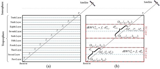
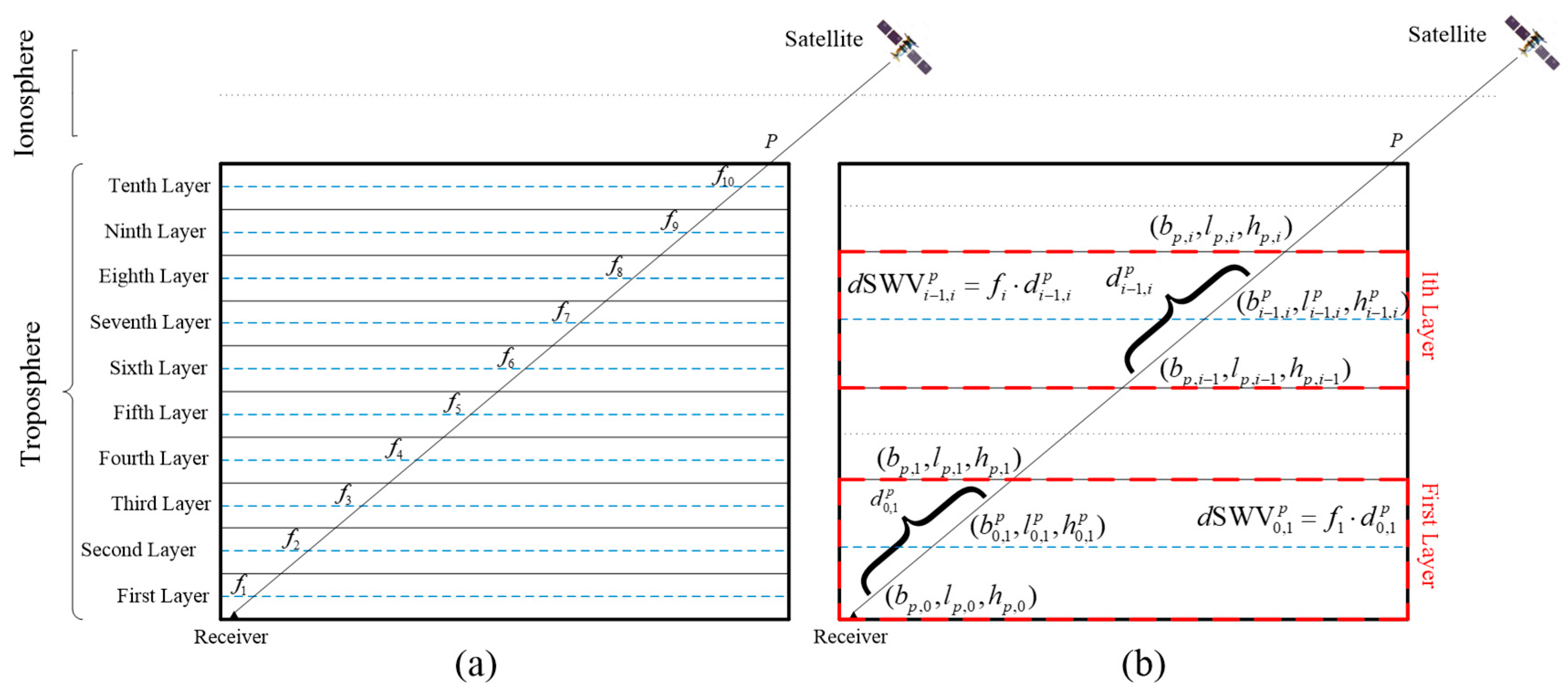
In this section, a tropospheric tomography approach is proposed which does not divide the research area in the horizontal direction, and only vertical layers are discretised (Figure 1). Considering the continuity of the spatial water vapour changes, a horizontal parameterised function is introduced for each layer to describe the water vapour change, and the water vapour density for each layer is replaced by the value at the layer’s centre. Several experiments have been tested and the expression of this horizontal parameterised function is determined according to the smallest root mean square (RMS) error of water vapor density differences between the actual water vapour density and the fitted values at different layers. The water vapour density at each layer’s centre can thus be expressed as:

$$\rho =f(b,l)=a_0+a_1\cdot b+a_2\cdot l+a_3\cdot bl+a_4\cdot b^2+a_5\cdot l^2+a_6\cdot b^{2}l+a_7\cdot b{l}^2$$

(4)

where $\rho$ represents the water vapor density. $a_0-a_7$ are the coefficients of water vapour density function, which are estimated and updated during the process of each tomographic resolution (Section 3); $b$ and $l$ are the latitude and longitude of intersection between the signal ray and the centre of the selected layer, respectively. Therefore, the value of SWV for the ith layer can be derived as:

$${\mathrm{S}}_{\mathrm{WV}(i-1,i)}^p={\rho }_i\cdot d_i^p=f(b_i,l_i)\cdot d_i^p$$

(5)

where ${\rho }_i$ is the water vapour density for the location of $(b_i,l_i)$ while the $d_i^p$ is the distance of satellite signal travelled to the $i\mathrm{th}$ layer, which can be calculated using the intersections of signal ray $p$ with two sides of the $i\mathrm{th}$ layer, as shown in Figure 1:

$$d_{i-1,i}^p=\{\begin{array}{cc}\sqrt{{(b_{p,i}-b_{p,0})}^2+{(l_{p,i}-l_{p,0})}^2+{(h_{p,i}-h_{p,0})}^2},& i=1;\\ \sqrt{{(b_{p,i}-b_{p,i-1})}^2+{(l_{p,i}-l_{p,i-1})}^2+{(h_{p,i}-h_{p,i-1})}^2},& i\ne 1;\end{array}$$

(6)

where $(b_{p,i},l_{p,i},h_{p,i})$ and $(b_{p,i-1},l_{p,i-1},h_{p,i-1})$ are the intersected coordinates of signal ray $p$ with the upper and lower boundaries of the $i\mathrm{th}$ layer, respectively, while $(b_{p,0},l_{p,0},h_{p,0})$ is the coordinate of the receiver. As described by [2], the observation equation of the tomography model can be regarded as a linear system, and therefore the total SWV of Equation (1) can be replaced by the following expression based on Equation (5):

$$\begin{array}{l}{\mathrm{S}}_{\mathrm{WV}}={\mathrm{S}}_{\mathrm{WV}(0,1)}+{\mathrm{S}}_{\mathrm{WV}(1,2)}+\cdots {\mathrm{S}}_{\mathrm{WV}(i-1,i)}+\cdots +{\mathrm{S}}_{\mathrm{WV}(n-2,n-1)}+{\mathrm{S}}_{\mathrm{WV}(n-1,n)}\\ ={10}^{-6}\left({\displaystyle {\int }_{h,0}^{h,1}{\rho }_{0,1}ds}+{\displaystyle {\int }_{h,1}^{h,2}{\rho }_{1,2}ds}+\cdots +{\displaystyle {\int }_{h,i-1}^{h,i}{\rho }_{i-1,i}ds}+\cdots +{\displaystyle {\int }_{h,n-2}^{h,n-1}{\rho }_{n-2,n-1}ds}+{\displaystyle {\int }_{h,n-1}^{h,n}{\rho }_{n-1,n}ds}\right)\end{array}$$

(7)

In our study, 10 layers are selected according to the principle demanding a smaller spacing in the lower layers and a larger spacing in the higher layers [13]. Consequently, the new observation equation of the proposed approach is as follows:

$$\begin{array}{l}{\mathrm{S}}_{\mathrm{WV}}={\mathrm{S}}_{\mathrm{WV}(0,1)}+{\mathrm{S}}_{\mathrm{WV}(1,2)}+\cdots +{\mathrm{S}}_{\mathrm{WV}(4,5)}+\cdots +{\mathrm{S}}_{\mathrm{WV}(8,9)}+{\mathrm{S}}_{\mathrm{WV}(9,10)}\\ =f_1\cdot d_{0,1}+f_2\cdot d_{1,2}+\cdots +f_5\cdot d_{4,5}+\cdots +f_9\cdot d_{8,9}+f_{10}\cdot d_{9,10}\\ ={10}^{-6}(a_{00}+a_{01}\cdot b_{0,1}+a_{02}\cdot l_{0,1}+a_{03}\cdot b_{0,1}{l}_{0,1}+a_{04}\cdot b_{0,1}^2+a_{05}\cdot l_{0,1}^2+a_{06}\cdot b_{0,1}^2{l}_{0,1}+a_{07}\cdot b_{0,1}{l}_{0,1}^2)\cdot d_{0,1}^p+\\ {10}^{-6}(a_{10}+a_{11}\cdot b_{1,2}+a_{12}\cdot l_{1,2}+a_{13}\cdot b_{1,2}{l}_{1,2}+a_{14}\cdot b_{1,2}^2+a_{15}\cdot l_{1,2}^2+a_{16}\cdot b_{1,2}^2{l}_{1,2}+a_{17}\cdot b_{1,2}{l}_{1,2}^2)\cdot d_{1,2}^p+\cdots +\\ {10}^{-6}(a_{40}+a_{41}\cdot b_{4,5}+a_{42}\cdot l_{4,5}+a_{43}\cdot b_{4,5}{l}_{4,5}+a_{44}\cdot b_{4,5}^2+a_{45}\cdot l_{4,5}^2+a_{46}\cdot b_{4,5}^2{l}_{4,5}+a_{47}\cdot b_{4,5}{l}_{4,5}^2)\cdot d_{4,5}^p+\cdots +\\ {10}^{-6}(a_{80}+a_{81}\cdot b_{8,9}+a_{82}\cdot l_{8,9}+a_{83}\cdot b_{8,9}{l}_{8,9}+a_{84}\cdot b_{8,9}^2+a_{85}\cdot l_{8,9}^2+a_{86}\cdot b_{8,9}^2{l}_{8,9}+a_{87}\cdot b_{8,9}{l}_{8,9}^2)\cdot d_{8,9}^p+\\ {10}^{-6}(a_{90}+a_{91}\cdot b_{9,10}+a_{92}\cdot l_{9,10}+a_{93}\cdot b_{9,10}{l}_{9,10}+a_{94}\cdot b_{9,10}^2+a_{95}\cdot l_{9,10}^2+a_{96}\cdot b_{9,10}^2{l}_{9,10}+a_{97}\cdot b_{9,10}{l}_{9,10}^2)\cdot d_{9,10}^p\end{array}$$

(8)

where $a_{00}-a_{97}$ are the estimated parameters of water vapour density function for each layer. By introducing the horizontal parameterised function, the water vapour density at any place can be calculated using the established function, rather than only the values in the divided voxels, which is a significant improvement when compared to previous methods.

2.3. Prior Constraint

Although the horizontal parameterised function has its advantages, it does not ensure that the vertical distribution of the water vapour field was correctly modelled. The main reason is that if the arbitrary two layers are exchanged, the total SWV value of the signal ray may change a little, but the 3-d water vapour structure has changed significantly. To solve this problem, a prior constraint is introduced. In our study, the mean water vapour density in different layers derived from radiosonde data for the first three days of the tomographic epoch were exploited. Those values were located at different layers are regarded as the prior constraint for the location of radiosonde station and are expressed as follows:

$$\begin{array}{l}{\rho }_k^{rs}=f_k(b_{k-1,k},l_{k-1,k})=a_{k0}+a_{k1}\cdot b_{k-1,k}+a_{k2}\cdot l_{k-1,k}+a_{k3}\cdot b_{k-1,k}{l}_{k-1,k}+\\ a_{k4}\cdot b_{k-1,k}^2+a_{k5}\cdot l_{k-1,k}^2+a_{k6}\cdot b_{k-1,k}^2{l}_{k-1,k}+a_{k7}\cdot b_{k-1,k}{l}_{k-1,k}^2\end{array}$$

(9)

where ${\rho }_k^{rs}$ is the imposed prior constraint using radiosonde data at the $k\mathrm{th}$ layer. $(b_{k-1,k},l_{k-1,k})$ is the coordinate of the point at the $k\mathrm{th}$ central layer for the location of the radiosonde station. Consequently, the final tomographic model for the proposed function approach is established as follows:

$$\left[\begin{array}{l}{\mathit{L}}_B\\ {\mathbf{\rho }}_P\end{array}\right]=\left[\begin{array}{l}{\mathit{B}}_{m1\times n}\\ {\mathit{P}}_{m2\times n}\end{array}\right]\cdot {\mathit{a}}_{n\times 1}+\left[\begin{array}{l}{\Delta }_{m1\times n}\\ {\Delta }_{m2\times n}\end{array}\right]$$

(10)

where $m1,m2$, and $n$ are the numbers of observation equation, priori equation and coefficients of the horizontal parameterised function remaining to be estimated, respectively. $\mathit{a}$ is the column vector of coefficients. $\mathit{B}$ and $\mathit{P}$ are the coefficient matrices of the observation equation and prior constraint equation, respectively. ${\mathit{L}}_B$ and ${\mathbf{\rho }}_P$ are the column vector of SWV observations and the prior mean water vapour density at different heights derived from radiosonde data, respectively. $\Delta$ is the noise in the tomographic model.

3. The Weights Strategy for Proposed Tomography Approach

As mentioned in [25], the optimal weights for different types of input equations are prerequisite to ensure the quality of the tomographic result. However, only the weights for different types of equations were considered for the previous studies while the weights for the same type information were ignored. In our study, the weights of both aspects are considered for the proposed tomographic approach.

3.1. Selection of the Weights for the Same Type of Equation

The total SWV content for each signal ray is related to the satellite elevation angle and length in the tomography area. Hence, the weighted function includes satellite elevation angle which is given as:

$$P_{E_{le}}={sin}^2(E_{le})$$

(11)

where $E_{le}$ is the satellite elevation angle. In the meantime, the weighted function related to length can be expressed as:

$$\begin{array}{c}{P}_{D_{ist}}=1/(1+D_{ist})\\ D_{ist}=\sqrt{{(b_{p,k}-b_{p,0})}^2+{(l_{p,k}-l_{p,0})}^2+{(h_{p,k}-h_{p,0})}^2}\end{array}\}$$

(12)

where $D_{ist}$ is the distance of signal ray in the tomography area, while $(b_{p,k},l_{p,k},h_{p,k})$ is the intersection point coordinates of the $p\mathrm{th}$ signal ray and the centre of the topmost $k$ layer. In addition, the tomographic observation equation consists of SWV observations derived from multiple epochs, which is evenly distributed in the two sides of the tomography epoch. Therefore, the weighted function related to time span is determined as:

$$\begin{array}{c}{P}_{T_{corr}}=cos(T_{corr})\\ T_{corr}=\frac{T_{obs}-T_{tom}}{(T_{interval}/2)}\end{array}\}$$

(13)

where $T_{obs}$ is the epoch of the observed SWV observation while $T_{tom}$ is the tomographic epoch. $T_{interval}$ is the selected tomographic period, in which the water vapour density is considered to be the same. Consequently, the final weighted function for each signal ray can be obtained as:

$$\begin{array}{l}{P}_i^B=P_{E_{le}}\cdot P_{D_{ist}}\cdot P_{T_{corr}}\\ ={sin}^2(E_{le})\cdot cos(T_{corr})/(1+D_{ist})\end{array}$$

(14)

The final weight matrix of the observation equation can be expressed as:

$${\mathit{P}}_B={\left[\begin{array}{ccccc}{p}_1^B& 0& \cdots & 0& 0\\ 0& p_2^B& & & 0\\ ⋮& & \ddots & & ⋮\\ 0& & & p_{m1-1}^B& 0\\ 0& 0& \cdots & 0& p_{m1}^B\end{array}\right]}_{m1\times m1}$$

(15)

where ${\mathit{P}}_B$ is the weight matrix of the observation equation. As for the weights for prior equation, the standard deviation (SD) at different layers derived from radiosonde data for the first three days before the tomographic epoch is used. As a result, the weight matrix for the prior constraint is expressed as:

$${\mathit{P}}_P={\left[\begin{array}{ccccc}{P}_1^P& 0& \cdots & 0& 0\\ 0& P_2^P& & & 0\\ ⋮& & \ddots & & ⋮\\ 0& & & P_{m2-1}^P& 0\\ 0& 0& \cdots & 0& P_{m2}^P\end{array}\right]}_{m2\times m2}$$

(16)

where $P_i^P=1/({s_{td}}^i\cdot {s_{td}}^i)$, ${s_{td}}^i$ is the SD calculated from radiosonde data.

3.2. Determination of the Weights for Different Types of Equations

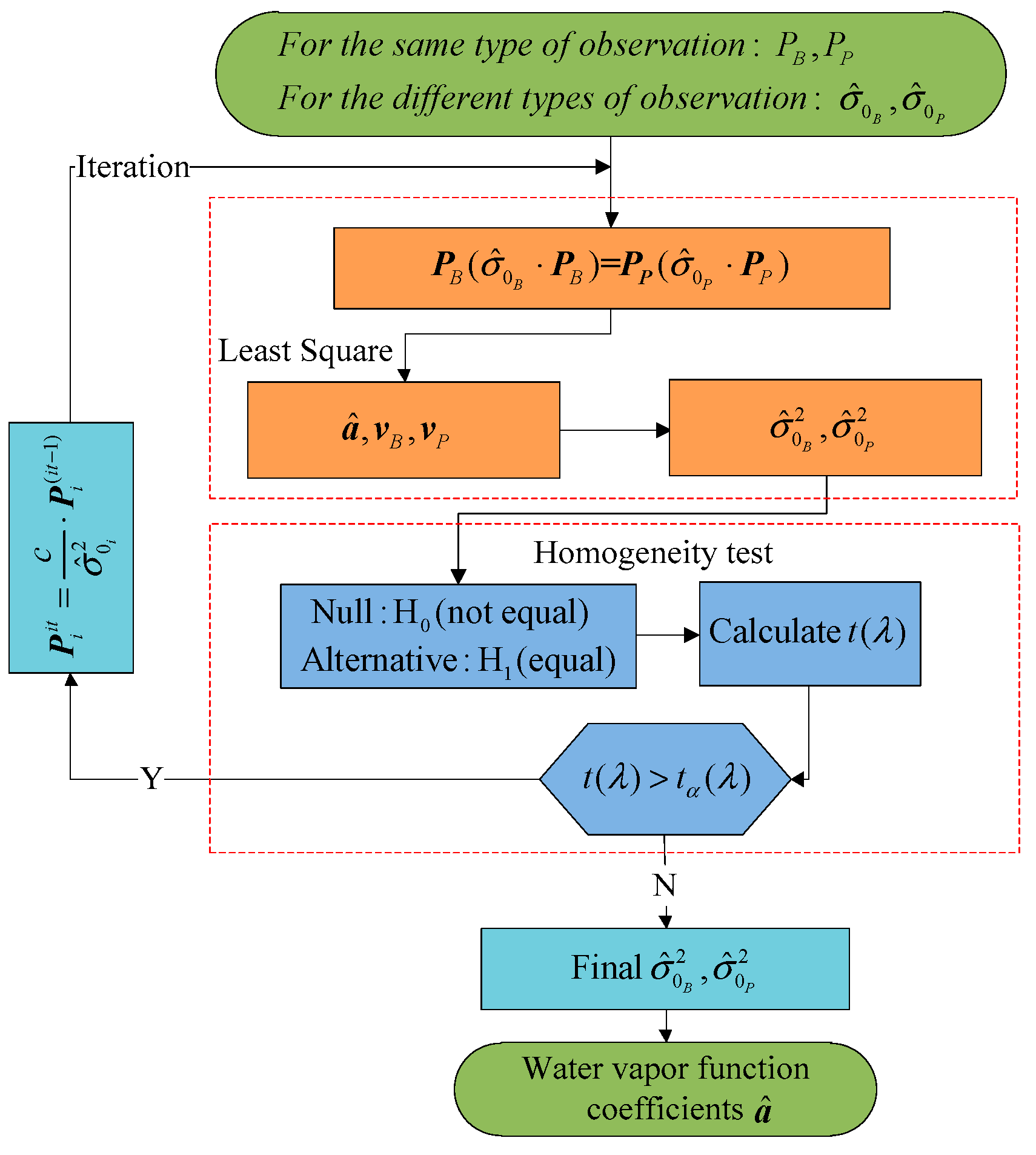
The covariance matrices for the two types of equations mentioned above are set as follows:

$${\mathit{D}=\mathit{P}}^{-1}=\left[\begin{array}{cc}{\mathit{D}}_B& 0\\ 0& {\mathit{D}}_P\end{array}\right]=\left[\begin{array}{cc}{\widehat{\sigma }}_{0_B}^2& 0\\ 0& {\widehat{\sigma }}_{0_P}^2\end{array}\right]\left[\begin{array}{cc}{\mathit{P}}_B^{-1}& 0\\ 0& {\mathit{P}}_P^{-1}\end{array}\right]$$

(17)

where ${\widehat{\sigma }}_{0_B}^2$ and ${\widehat{\sigma }}_{0_P}^2$ are the unit weight variances for two types of equations, which are calculated based on the method of variance components estimation [26]. The flowchart of determining the optimal weights is presented in Figure 2 and the detailed steps are also given below.

(1)

Set the initial value of unit weight variance for different equations as the same, for example 1 is selected in our study.

(2)

Conduct adjustment using the least squares method for Equation (10) and obtain the posteriori residuals of observation equation and priori equation (${\mathit{v}}_B$ and ${\mathit{v}}_P$).

(3)

Calculate the new posteriori unit weight variance ${\widehat{\sigma }}_{0_B}^2$ and ${\widehat{\sigma }}_{0_P}^2$ for two kinds of inputs according to the following formulae [26,27]:

$$\begin{array}{c}{\widehat{\sigma }}_{0_i}^2=\frac{{\mathit{v}}_i^T{\mathit{P}}_i{\mathit{v}}_i}{l_i-tr({\mathit{N}}^{-1}{\mathit{N}}_i)}\\ \mathit{N}={\mathit{A}}^{T}PA\\ {\mathit{N}}_i={\mathit{A}}_i^T{\mathit{P}}_i{\mathit{A}}_i\\ \mathit{A}={\left[\begin{array}{cc}{\mathit{A}}_B& {\mathit{A}}_P\end{array}\right]}^T\end{array}\}$$

(18)

where $l(i=1,2)$ is the number of two types of input equations.

(4)

Decide whether the unit weight variances ${\widehat{\sigma }}_{0_B}^2$ and ${\widehat{\sigma }}_{0_P}^2$ are equal or not. In our study, the homogeneity test is used on the principle that the estimated variance components are statistically equal [25,28]. In Figure 2, ${\mathrm{H}}_0$ represents the case when the calculated posteriori unit weight variances are not equal while ${\mathrm{H}}_1$ refers to the opposite case.

(5)

Adjust and update the weight matrices according to the formula below and repeat Steps (2) to (4) until the relationship between the calculated ${\widehat{\sigma }}_{0_B}^2$ and ${\widehat{\sigma }}_{0_P}^2$ in Step (4) satisfies the termination criteria for statistical equality.

$${\mathit{P}}_i^{\phi }=\frac{c}{{\widehat{\sigma }}_{0_i}^2}\cdot {\mathit{P}}_i^{(\phi -1)}$$

(19)

where $\phi$ is the number of iterations, and $c$ is an arbitrary constant which takes the value of ${\widehat{\sigma }}_{0_B}^2$.

4. Validation of the Horizontal Parameterised Approach

4.1. Processing Strategy

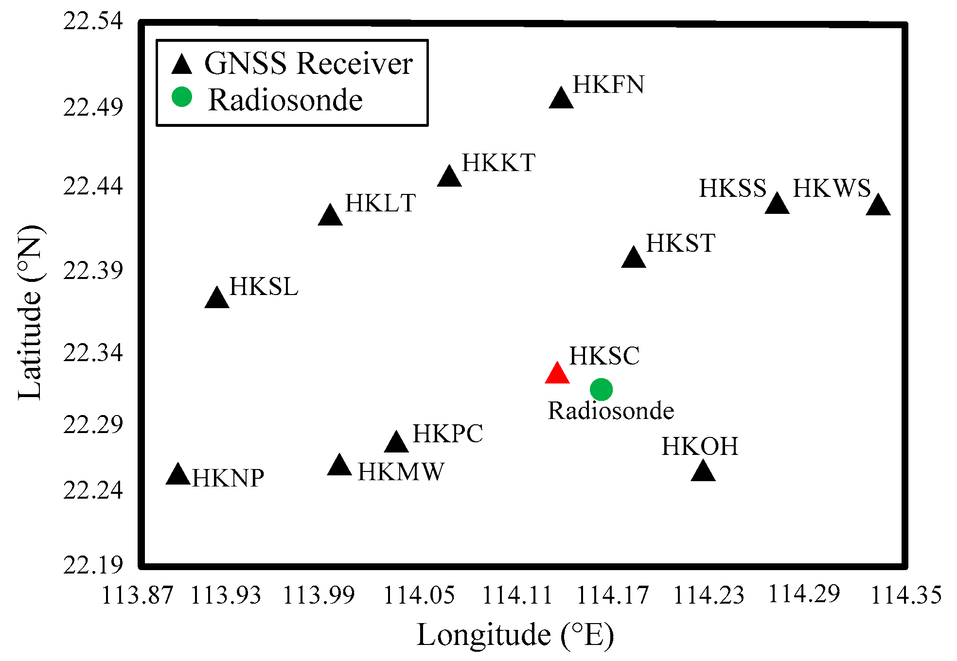
The GPS data of 12 ground-based receivers (black and red triangles in Figure 3) obtained from the SatRef in Hong Kong are selected for the period of Doy (Day of Year) 121–151, 2013. Figure 3 shows the geographic distribution of GNSS receivers for the experimental area, where the red triangle (HKSC) is also a GNSS receiver used to validate the proposed method in Section 4.2.2. As mentioned above, the observed data were processed using GAMIT/GLOBK (v10.5) based on the double-differenced combined observation. [29] proposed that some stations with baselines longer than 500 km should be included for a regional network resolution if the absolute tropospheric parameters need to be estimated. Therefore, three International GNSS Service (IGS) stations (SHAO, BJFS and LHAZ) were also considered for the data processing. The sampling interval for the observed GPS data is 30 s, while the intervals of estimated ZTD and the gradient parameters are 0.5 h and 2 h, respectively. The gradient component includes the parameters in east–west and south–north directions and the GMF is used during the process of GPS observation [24].

The time span selected for each tomographic resolution in which the water vapour density is assumed to be a constant is 5 min. The tomography area ranges from 113.87°E to 113.45°E and 22.19°N to 22.54°N in longitudinal and latitudinal directions, respectively. The boundary of the tomography area is 10 km with non-uniform thicknesses of 0.6, 0.6, 0.8, 0.8, 1.0, 1.0, 1.0, 1.4, 1.4, and 1.4 km from bottom to top, respectively [13]. As shown in Figure 3, there is a radiosonde station (green circle) in the research area, where the sounding balloon is launched automatically at 00:00 and 12:00 UTC daily. In addition, some ECMWF grid points are also distributed in this area with a spatial resolution of 0.125° × 0.125° while the temporal resolution is four times a day at 00:00, 06:00, 12:00, and 18:00 UTC, respectively. The coordination information of ECMWF grid points is given in

Table 1. Geographic coordination of European Centre for Medium-Range Weather Forecasts (ECMWF) grid points located in the selected area.

Number	Longitude (°E)	Latitude (°N)	Number	Longitude (°E)	Latitude (°N)
1	113.875	22.250	7	114.125	22.375
2	114.000	22.250	8	114.250	22.375
3	114.125	22.250	9	113.875	22.500
4	114.250	22.250	10	114.000	22.500
5	113.875	22.375	11	114.125	22.500
6	114.000	22.375	12	114.250	22.500

. Radiosonde and ECMWF data are both used in the following sections to validate the proposed tomographic model due to their ability to obtain accurate water vapour density profiles at different altitudes [19,30,31].

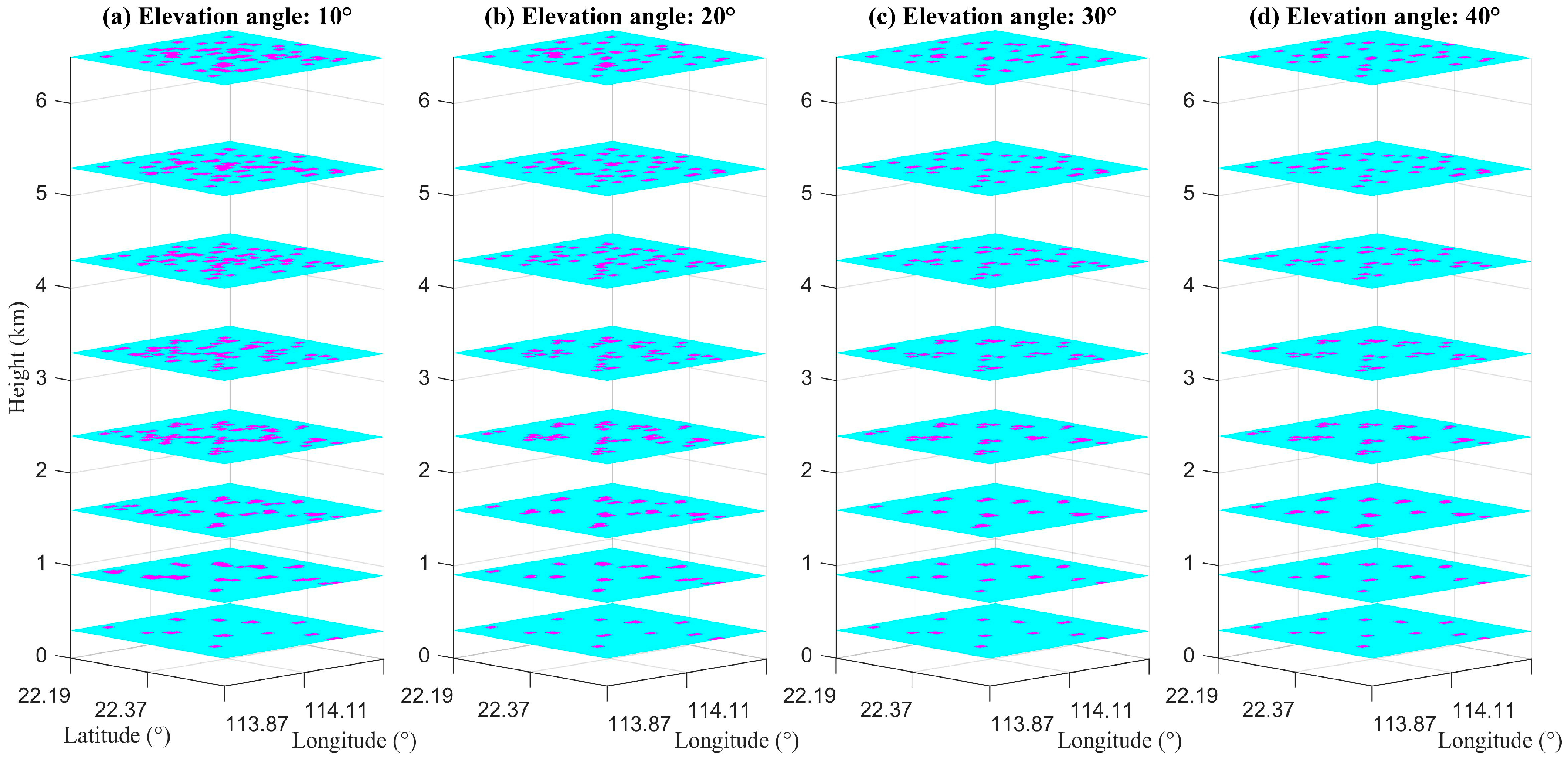
As mentioned above, the proposed approach only uses those signal rays with a large elevation angle. The following gives the principle of determining the smallest threshold of satellite elevation angle masks. Figure 4 shows the distribution of intersections between signal rays and one to eight layers for the period of 00:00–00:05 UTC, Doy 121, 2013. Here, elevation angles of 10°, 20°, 30° and 40° are selected (Figure 4a–d). It can be observed from Figure 4 that the number of intersections decreased with elevation angle masked increases in the upper layers. However, the distributions of intersections from Figure 4a–d are similar in the lower layers. Due to the water vapor content being mainly concentrated on the low atmosphere, the principle of determining the satellite elevation angle masks we followed is that the angle masks can guarantee sufficient intersections evenly distributed in each layer, especially for the low layers. By analysing the distribution of intersections over the experimental period, it is found that an elevation angle mask of 30° satisfies the requirement, which we used hereafter in the following experiment. [32] proved that, when the elevation angle masks exceed 15°, the ray path can be assumed linear and the influence of ray bending can be neglected. Therefore, it is acceptable to ignore the impact of ray bending on the tomographic result in our experiment.

4.2. Evaluation of the Proposed Tomographic Model

The accuracy of the novel tomographic model is first evaluated under different weather conditions. Two days (Doy 138 and 146) are selected because those two days correspond to different weather conditions (a sunny day on Doy 138 and a rainy day on Doy 146, respectively) according to the weather records of the Hong Kong Observatory.

4.2.1. Internal Accuracy Validation

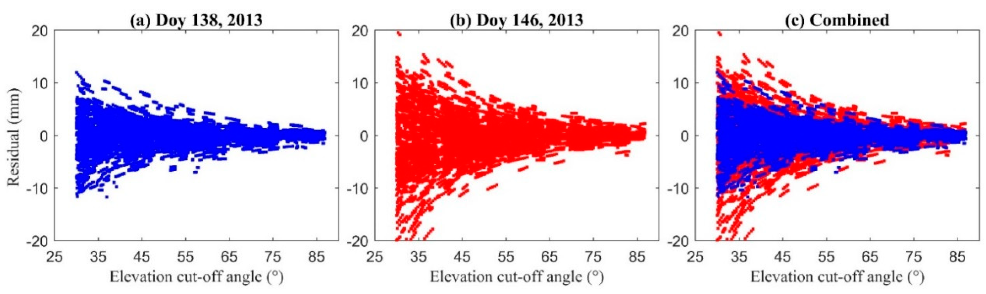
To test the performance of the novel tomographic model, the SWV observations with elevation angle masks of 30° are calculated using the water vapour density derived from the proposed approach and their discrepancies are compared against the calculated SWV values based on GPS observations. Figure 5 shows how the residuals change with elevation angle for two different weather conditions, where the blue and red dot represent the residuals calculated for a sunny and a rainy day with standard deviation error (SE) values of 2.4 mm and 4.1 mm, respectively. It can be observed that the SE is relatively large during the rainy day. This is because the water vapour content is large and relatively active on a rainy day compared to that on a sunny day.

4.2.2. External Accuracy Validation

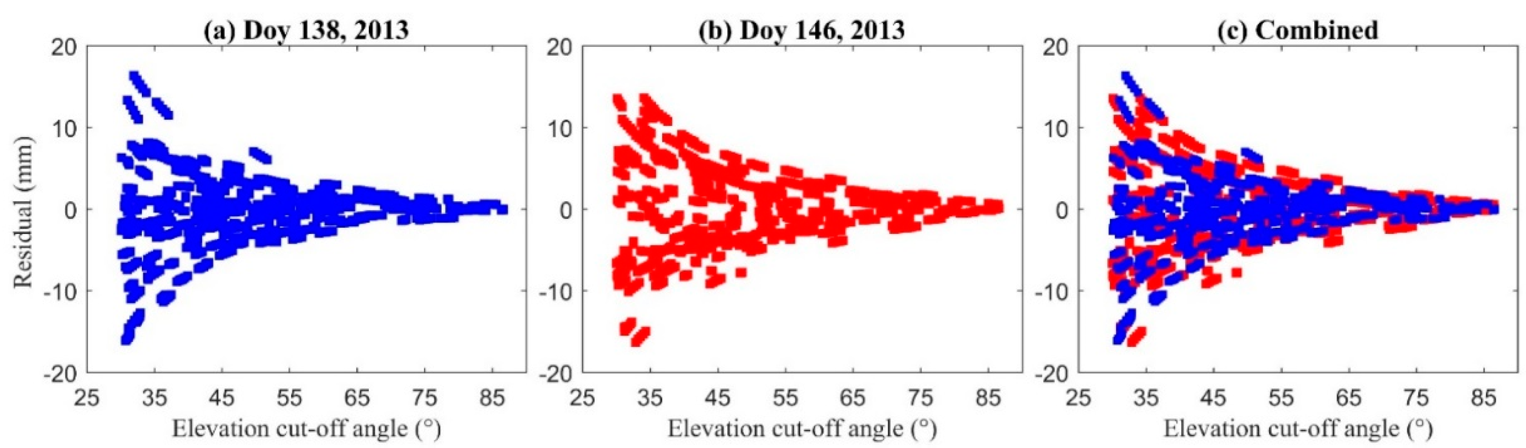
To further assess the novel tomographic model, another experiment is conducted in which only eleven stations were used (black triangles in Figure 3) in SatRef while the HKSC station (red triangle in Figure 3) was selected as a reference. Figure 6 shows the residuals of SWV observations with an elevation angle mask of 30° for HKSC station on a sunny and a rainy day, respectively. The blue dot represents the residuals of SWV values on the sunny day, and the values of SE, maximum, and minimum were 3.9 mm, 16.4 mm, and −16.1 mm, respectively, while the red dot represents the residuals on a rainy day, and the values of SE, maximum, and minimum were 4.6 mm, 13.6 mm, and −16.3 mm, separately.

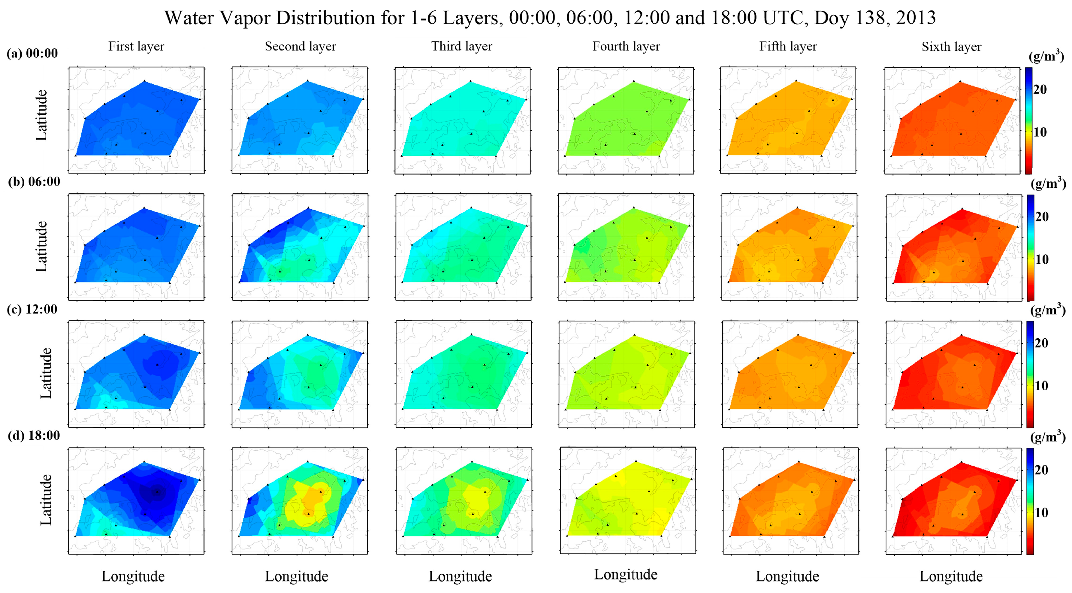
According to the external/internal accuracy validation of the novel tomographic model on a sunny and on a rainy day, we can conclude that the proposed approach is stable and applicable. In addition, the reconstructed result of the proposed approach showed slightly better accuracy for GPS tropospheric tomography on a sunny day, compared to that on a rainy day. The water vapor distributions at 00:00, 06:00, 12:00 and 18:00 UTC, Doy 138 in layers of 1–6 are also presented derived from the proposed method (Figure 7), from which the spatio-temporal variations in water vapor density for different layers can be clearly observed. Additionally, it can be found from Figure 7 that the water vapor is mainly concentrated on the bottom layers and decreased with the increasing of altitude but was non-uniform.

4.3. Comparison with the Traditional Tomographic Method

To validate the performance of the proposed method, the tomographic results are compared with that from the traditional method in this section while the radiosonde and ECMWF data are regarded as the references, respectively. For traditional tomography, the horizontal resolutions in latitudinal and longitudinal directions are 0.05° and 0.06°, respectively, while the vertical height is selected as 10 km with the same division described by the proposed method. Therefore, the total number of voxels is 7 × 8 × 10. Here, two schemes are determined to compare the tomographic results conveniently. Scheme 1 refers to the traditional method while scheme 2 represents the proposed method in the following comparison.

4.3.1. Uniformity of the Height System

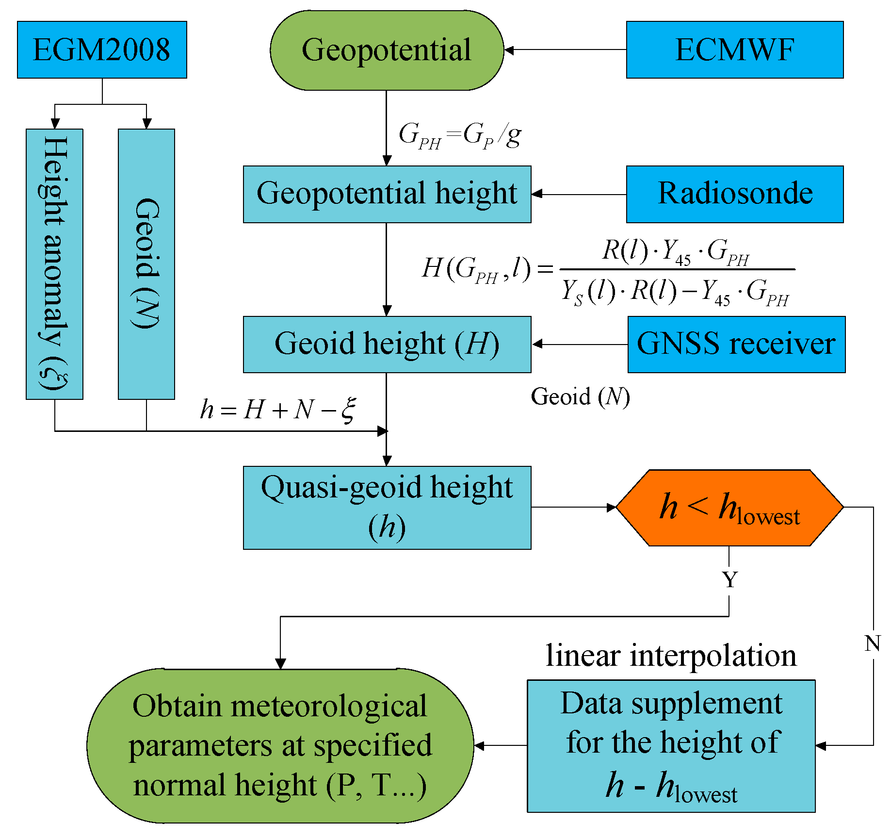
Before calculating the water vapour density at different heights for the location of radiosonde station or ECMWF grid points, the height system must first be unified. In our study, the normal height system was used. The following height conversion steps to change from geopotential to quasi-geoid height were used, while Figure 8 shows the flowchart for conversion between different height systems:

(1)

Converting geopotential to geopotential height [33]:

$$G_{PH}{=G}_P/g$$

(20)

where $G_P$ represents geopotential while $G_{PH}$ represents geopotential height. $g$ is the local gravitational acceleration with a constant value of 9.80665 m/s².

(2)

Converting geopotential height to geoid height according to the formulae below [33,34,35]:

$$H(G_{PH},l)=\frac{R(l)\cdot Y_{45}\cdot G_{PH}}{Y_S(l)\cdot R(l)-Y_{45}\cdot G_{PH}}$$

(21)

where $H$ is the ellipsoid height. $Y_S(l)$ represents the normal gravitational acceleration on the surface of the ellipsoid of revolution while $R(l)$ is an effective radius of the Earth for latitude $l$. $Y_{45}$ is the normal gravitational acceleration on the surface of the ellipsoid for latitude 45° (9.80665 m/s²); and $Y_S(l)$ and $R(l)$ can be calculated from [33]:

$$Y_S(l)=9.780325\cdot {\left[\frac{1+0.00193185\cdot \sin {(l)}^2}{1-0.00669435\cdot \sin {(l)}^2}\right]}^{0.5}$$

(22)

$$R(l)=\frac{6378.137}{1.006803-0.006706\cdot \sin {(l)}^2}$$

(23)

(3)

Converting geoid height to quasi-geoid height using the official Earth Gravitational Model 2008 (EGM 2008) derived from the U.S. National Geospatial-Intelligence Agency EGM Development Team [36]:

$$h=H+N-\xi$$

(24)

where $h$ represents the quasi-geoid height. $N$ and $\xi$ are the geoid and height anomaly, respectively, which are both derived from EGM 2008.

(4)

Judging whether the height of radiosonde data ($h_{lowest}$) was lower than that of the receiver ($h$) or not, and then performing vertical extrapolation for height $h-h_{lowest}$ [37,38] or neglect this step.

4.3.2. Integrated Water Vapour (IWV) Comparison

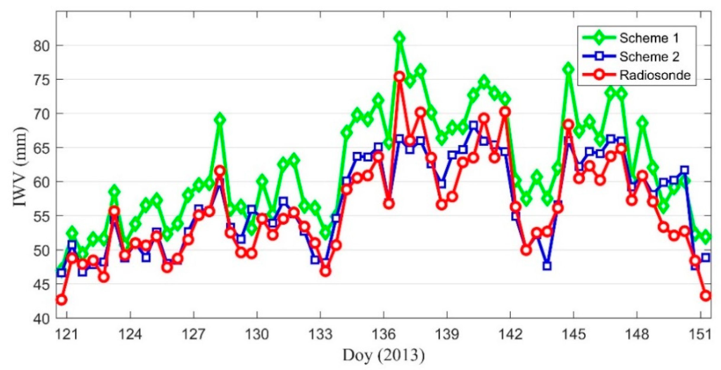
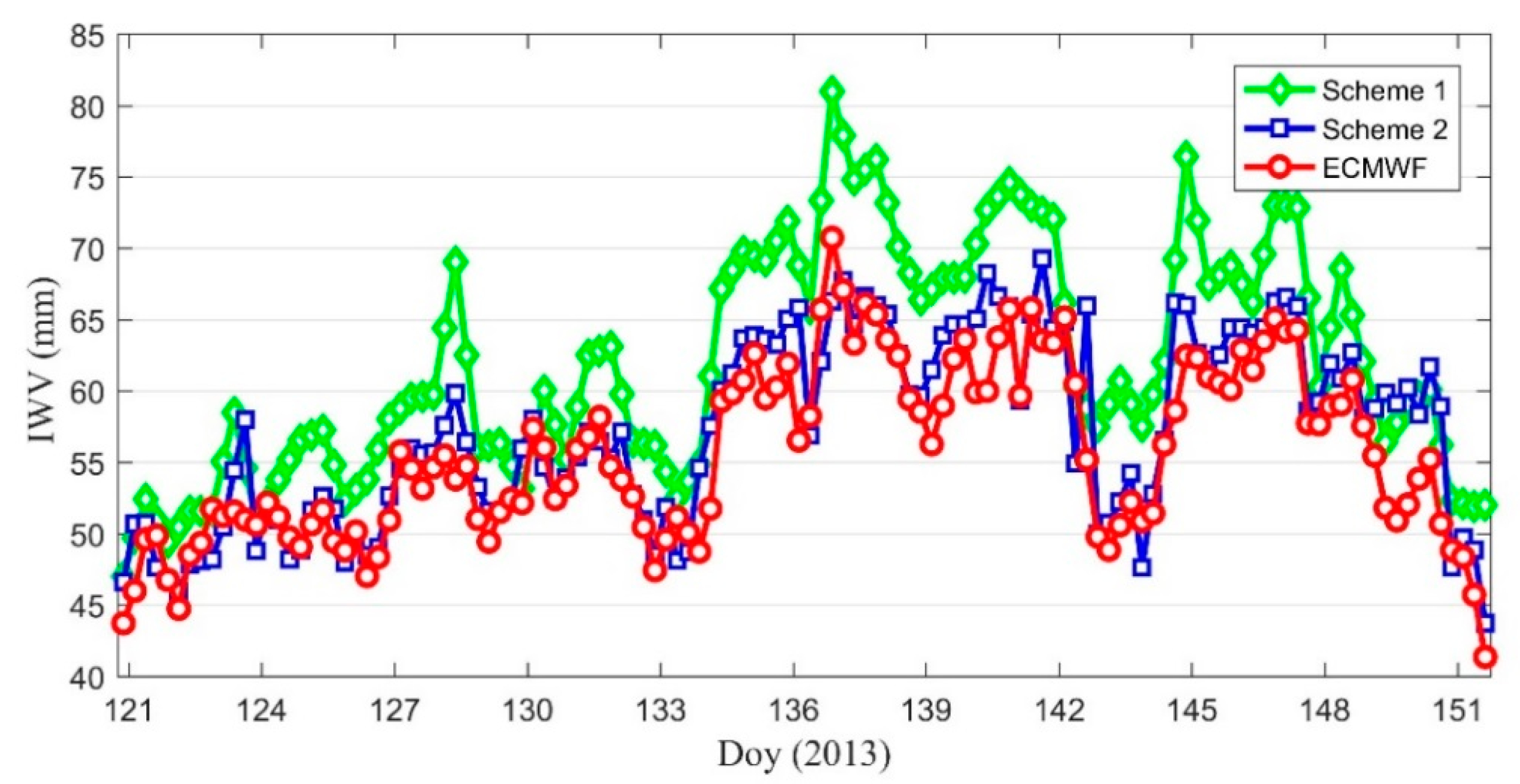
Here, the IWV values integrated along the vertical direction using the reconstructed water vapour density derived from different tomographic schemes for the location of radiosonde station are compared with those obtained from the radiosonde data. Figure 9 shows the IWV comparison between the different tomographic schemes and radiosonde data at epochs 00:00 and 12:00 UTC on each day of the period Doy 121–151, 2013. In addition, the IWV time series are also compared with those derived from ECMWF data. The IWV time series of ECMWF for the location of radiosonde station are calculated using the data derived from the surrounding ECMWF grid points based on the inverse distance weighted (IDW) method [39]. Figure 10 shows the IWV comparison between the different tomographic schemes and ECMWF at epochs 00:00, 06:00, 12:00 and 18:00 UTC on each day of the experimental period.

Figure 9 and Figure 10 show that the IWV time series derived from schemes 1 and 2 are consistent with those from radiosonde and ECMWF data for most epochs, respectively. According to the statistical results over the period of 31 days (

Table 2. Statistical result of IWV comparison for 31 days, unit: (mm).

Statistical Result	Root Mean Square (RMS)	Bias
Scheme 1 vs. Radiosonde	5.1	−3.9
Scheme 2 vs. Radiosonde	3.2	−0.8
Scheme 1 vs. ECMWF	6.3	−5.9
Scheme 2 vs. ECMWF	3.3	−1.7

), the RMS/Bias of IWV differences between scheme 1 and radiosonde are 5.1/−3.9 mm, respectively, while the values are 6.3/−5.9 mm, separately between scheme 1 and ECMWF data. Evidently, the corresponding RMS/Bias are small for the proposed method in this paper when compared to the radiosonde data (3.2/−0.8 mm) and ECMWF data (3.3/−1.7 mm), respectively.

4.3.3. Water Vapour Profile Comparison

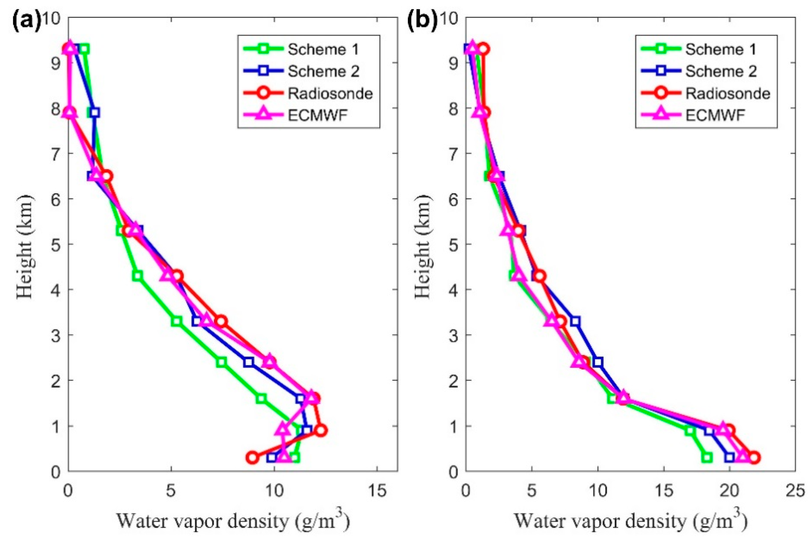
The IWV is an integrated water vapour value which cannot reflect the layered distribution of water vapour density, although the IWV time series derived from the proposed tomographic approach are superior to the traditional method, the 3-d distribution of water vapour density still needed to be further verified. Therefore, two epochs are selected to compare the water vapour profile derived from different tomographic schemes; those schemes refer to the traditional tomographic method (Scheme 1) and the method proposed in this paper (Scheme 2). Figure 11 shows the water vapour density profile comparison derived from different tomographic schemes, radiosonde and ECMWF data over two epochs, 00:00 UTC, Doy 122 and 00:00 UTC, Doy 135, 2013, respectively.

It can be observed from Figure 11 that the water vapour density profiles derived from different tomographic schemes, radiosonde, and ECMWF data match each other at most heights. However, the water vapor profiles derived from scheme 2 have a higher consistence with radiosonde and ECMWF data than that from scheme 1. In addition, the differences in water vapour density at most altitudes for tomography–radiosonde and tomography–ECMWF are relatively small at 00:00 UTC, Doy 122, compared to that at 00:00 UTC, Doy 135; this is because the water vapour content is relatively low (less than 15 g/m³ in the lowest layer at date 00:00 UTC, Doy 122) while it is greater than 20 g/m³ in the lowest layer at 00:00 UTC, Doy 135. Statistical analysis reveals that the RMS/Bias of differences of water vapor density for scheme 1–radiosonde and scheme 1–ECMWF at 00:00 UTC, Doy 122 are 1.65/0.64 g/m³ and 2.10/−1.32 g/m³, respectively, while the values at 00:00 UTC, Doy 135 were 1.38/−0.48 g/m³ and 1.23/−0.57 g/m³, respectively. For scheme 2, the values of RMS /Bias are 0.80/0.13 g/m³ and 0.98/0.20 g/m³, respectively, at 00:00 UTC, Doy 122 and 0.75/−0.03 g/m³ and 1.00/−0.34 g/m³, respectively, at 00:00 UTC, Doy 135, when compared with the radiosonde and ECMWF data.

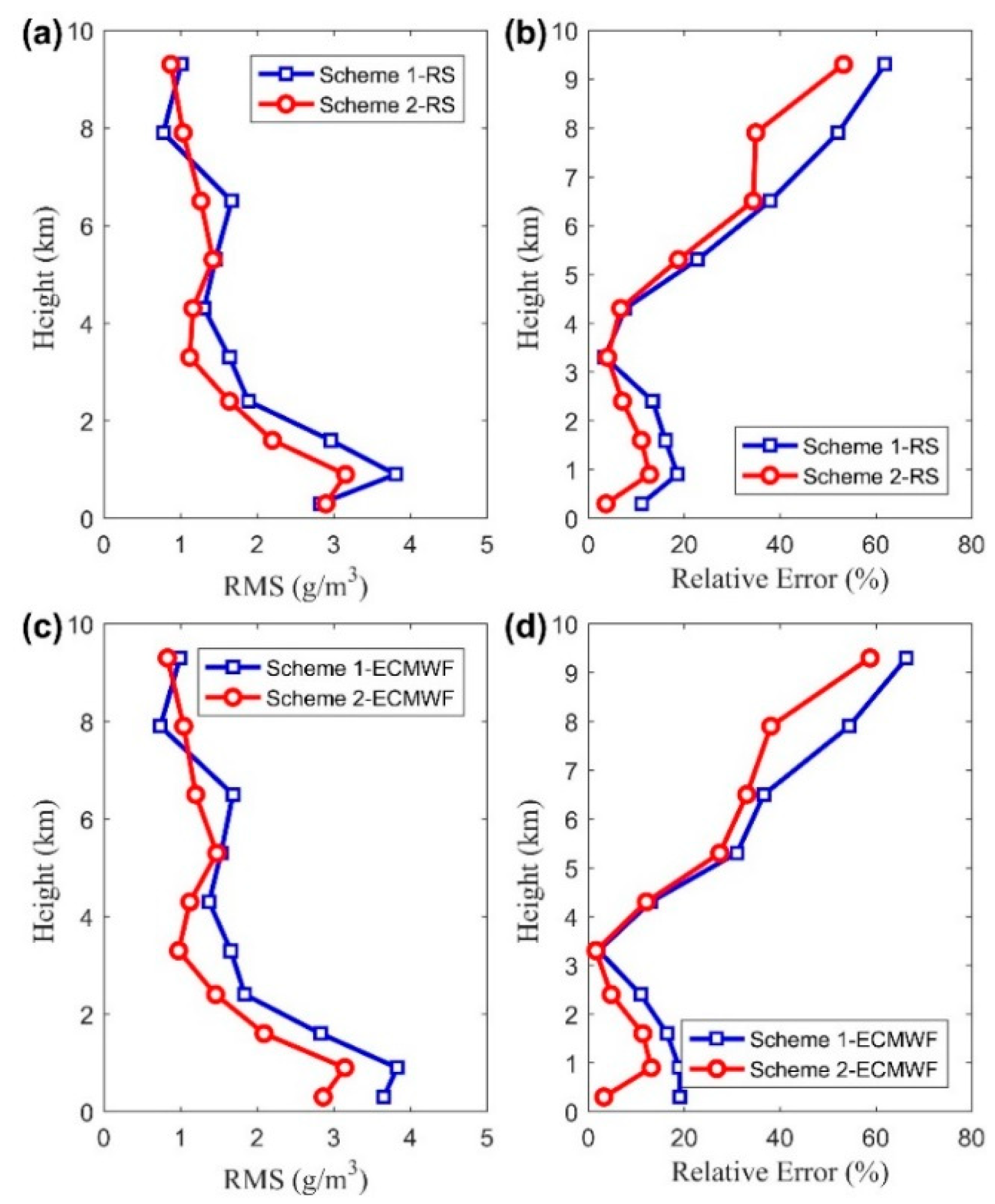
The 31-day test is carried out to analyse the accuracy of water vapour density at different altitudes. The relative discrepancy of water vapor density derived from different schemes, radiosonde and ECMWF data is introduced to reflect the relationship of the proposed approach and its error with height [40]. The following gives the formula for calculating the relative error:

$$R_e=\frac{|W_{VD}-W_{VD}^0|}{W_{VD}^0}$$

(25)

where $R_e$ is the relative error. $W_{VD}$ is the water vapor density value derived from different tomographic schemes. $W_{VD}^0$ is the water vapor density value derived from radiosonde or ECMWF.

Figure 12 presents the RMS and relative error derived from different tomographic results, radiosonde and ECMWF during the experimental period from Doy 121 to 151, 2013. It can be concluded from Figure 12a,c that the RMS of water vapour density differences at most heights between scheme 2-radiosonde and scheme 2-ECMWF are superior to that derived from scheme 1–radiosonde and scheme 1–ECMWF, respectively. A similar conclusion is also obtained by comparing the relative error in Figure 12b,d. Statistical results for the period of 31 days (

Table 3. Statistical result of water vapor density profile comparison for 31 days, unit: (g/m³).

Statistical Result	RMS	Bias
Scheme 1 vs. Radiosonde	1.33	0.38
Scheme 2 vs. Radiosonde	0.88	0.06
Scheme 1 vs. ECMWF	1.59	0.40
Scheme 2 vs. ECMWF	0.92	−0.08

) shows that the RMS errors in the water vapour field from the traditional method are about 1.33 g/m³ and 1.59 g/m³, respectively, when compared to the radiosonde and ECMWF data; however, the RMS errors of the proposed method in this paper are 0.88 g/m³ and 0.92 g/m³ when compared to radiosonde and ECMWF data. Therefore, the above comparison further demonstrates the superiority of the proposed method.

5. Conclusions

A horizontal parameterised approach is proposed for water vapour reconstruction and its ability and applicability have been validated under different weather conditions and over 31 days. The proposed approach divided the research area into layers vertically while the water vapour density function is introduced horizontally, rather than discretising the research area into many voxels as in previous studies [2,9,10,11,12,41], which is the innovation of this paper. By using the proposed approach, empirical assumptions imposed on the inner divided voxels are neglected. The proposed method also avoids unfavourable effects on the tomographic result due to the improper relationship between voxels in the vertical and horizontal constraints. Additionally, another novel aspect of the proposed method is that the estimated parameters decreased as only the coefficients of the horizontal parameterised function for each layer are estimated, which overcame the rank deficiency problem during tomographic resolution. Moreover, only those observations with elevation angle masks of greater than the given threshold, e.g., 30°, are selected and used as input information, which effectively overcame the problem that the tomographic result is subjected to the effect of signal rays of low elevation angle due to their relatively low-accuracy observations when compared to signal rays of high elevation angles.

By comparing the residuals of SWV values, we found that the SE of SWV differences were 2.4 mm and 4.1 mm for the internal test, while values of 3.9 mm and 4.6 mm are obtained using the HKSC station data for an external test under two different types of weather conditions (a sunny and a rainy day). Tomographic results of both traditional and proposed methods for 31 days are compared with IWV and water vapor density derived from radiosonde and ECMWF, respectively, and the result indicates the superiority of the proposed method both in IWV and water vapor density aspects when compared to the traditional method. Some validations of the proposed approach should focus on different research areas to further explore its ability. The elevation angle masks should be investigated if more satellite observations derived from different operational GNSS (GPS, GLONASS, GALILEO, and BDS) systems are used in the near future. In addition, some observed external information, such as observations from lidar, solar spectrometers, and Interferometric Synthetic Aperture Radar (InSAR), should be considered for possible assimilation into the proposed tomographic method, which are expected to enhance the ability of reconstructing the 3-d distribution of water vapour fields in the future.

References

- Braun, J.; Rocken, C.; Meertens, C.; Ware, R. Development of a water vapor tomography system using low cost L1 GPS receivers. Proc. Ninth Anrruai ARM Sci. Team Meet. 1999, 2226, 1–6. [Google Scholar]
- Flores, A.; Ruffini, G.; Rius, A. 4D tropospheric tomography using GPS slant wet delays. Ann. Geophys. 2000, 18, 223–234. [Google Scholar] [CrossRef] [Green Version]
- Seko, H.; Shimada, S.; Nakamura, H.; Kato, T. 3-d distribution of water vapor estimated from tropospheric delay of GPS data in a mesoscale precipitation system of the Baiu front. Earth Planets Space 2000, 52, 927–933. [Google Scholar] [CrossRef]
- Eriksson, D.; MacMillan, D.S.; Gipson, J.M. Tropospheric delay ray tracing applied in VLBI analysis. J. Geophys. Res. Solid Earth 2014, 119, 9156–9170. [Google Scholar] [CrossRef] [Green Version]
- Hofmeister, A.; Böhm, J. Application of ray-traced tropospheric slant delays to geodetic VLBI analysis. J. Geodesy 2017, 91, 945–964. [Google Scholar] [CrossRef] [Green Version]
- Hirahara, K. Local GPS tropospheric tomography. Earth Planets Space 2000, 52, 935–939. [Google Scholar] [CrossRef] [Green Version]
- Troller, M.; Bürki, B.; Cocard, M.; Geiger, A.; Kahle, H.G. 3-D refractivity field from GPS double difference tomography. Geophys. Res. Lett. 2000, 29, 1–4. [Google Scholar] [CrossRef]
- Skone, S.; Hoyle, V. Troposphere modeling in a regional GPS network. J. Glob. Position. Syst. 2005, 4, 230–239. [Google Scholar] [CrossRef]
- Nilsson, T.; Gradinarsky, L. Water vapor tomography using GPS phase observations: Simulation results. IEEE Trans. Geosci. Remote Sens. 2006, 44, 2927–2941. [Google Scholar] [CrossRef]
- Bender, M.; Raabe, A. Preconditions to ground based GPS water vapour tomography. Ann. Geophys. 2007, 25, 1727–1734. [Google Scholar] [CrossRef] [Green Version]
- Perler, D.; Geiger, A.; Hurter, F. 4D GPS water vapor tomography: New parameterised approaches. J. Geodesy 2011, 85, 539–550. [Google Scholar] [CrossRef]
- Brenot, H.; Walpersdorf, A.; Reverdy, M.; Van Baelen, J.; Ducrocq, V.; Champollion, C.; Giroux, P. A GPS network for tropospheric tomography in the framework of the Mediterranean hydrometeorological observatory Cévennes-Vivarais (southeastern France). Atmos. Meas. Tech. 2014, 7, 553–578. [Google Scholar] [CrossRef] [Green Version]
- Yao, Y.; Zhao, Q. A novel, optimized approach of voxel division for water vapor tomography. Meteorol. Atmos. Phys. 2016, 129, 57–70. [Google Scholar] [CrossRef]
- Xia, P.; Cai, C.; Liu, Z. GNSS troposphere tomography based on two-step reconstructions using GPS observations and COSMIC profiles. Ann. Geophys. 2013, 31, 1805–1815. [Google Scholar] [CrossRef] [Green Version]
- Alshawaf, F. Constructing Water Vapor Maps by Fusing InSAR, GNSS and WRF Data. Ph.D. Dissertation, Karlsruhe Institute of Technology, Karlsruhe, Baden-Württemberg, Germany, 2013. [Google Scholar]
- Heublein, M.; Zhu, X.X.; Alshawaf, F.; Mayer, M.; Bamler, R.; Hinz, S. Compressive sensing for neutrospheric water vapor tomography using GNSS and InSAR observations. Geosci. Remote Sens. Symp. (IGARSS) 2015, 5268–5271. [Google Scholar] [CrossRef] [Green Version]
- Benevides, P.; Nico, G.; Catalao, J.; Miranda, P. Merging SAR interferometry and GPS tomography for high-resolution mapping of 3D tropospheric water vapour. Geosci. Remote Sens. Symp. (IGARSS) 2015, 3607–3610. [Google Scholar] [CrossRef]
- Jiang, P.; Ye, S.R.; Liu, Y.Y.; Zhang, J.J.; Xia, P.F. Near real-time water vapor tomography using ground-based GPS and meteorological data: Long-term experiment in Hong Kong. Ann. Geophys. 2014, 32, 911–923. [Google Scholar] [CrossRef] [Green Version]
- Yao, Y.B.; Zhao, Q.Z.; Zhang, B. A method to improve the utilization of GNSS observation for water vapor tomography. Ann. Geophys. 2016, 34, 143–152. [Google Scholar] [CrossRef] [Green Version]
- Bender, M.; Dick, G.; Ge, M.; Deng, Z.; Wickert, J.; Kahle, H.G.; Tetzlaff, G. Development of a GNSS water vapour tomography system using algebraic reconstruction techniques. Adv. Space Res. 2011, 47, 1704–1720. [Google Scholar] [CrossRef] [Green Version]
- Bevis, M.; Businger, S.; Herring, T.A.; Rocken, C.; Anthes, R.A.; Ware, R.H. GPS meteorology: Remote sensing of atmospheric water vapor using the Global Positioning System. J. Geophys. Res. Atmos. 1992, 97, 15787–15801. [Google Scholar] [CrossRef]
- Chen, Y.Q.; Liu, Y.X.; Wang, X.Y.; Li, P.H. GPS real-time estimation of precipitable water vapor-Hong Kong experiences. Acta Geod. Cartogr. Sin. 2007, 36, 9–12. [Google Scholar]
- Herring, T.A.; King, R.W.; McClusky, S.C. Documentation of the GAMIT GPS Analysis Software Release 10.4; Department of Earth and Planetary Sciences, Massachusetts Institute of Technology: Cambridge, MA, USA, 2010. [Google Scholar]
- Böhm, J.; Niell, A.; Tregoning, P.; Schuh, H. Global Mapping Function (GMF): A new empirical mapping function based on numerical weather model data. Geophys. Res. Lett. 2006, 33, 1–4. [Google Scholar] [CrossRef]
- Guo, J.; Yang, F.; Shi, J.; Xu, C. An optimal weighting method of global positioning system (GPS) troposphere tomography. IEEE J. Sel. Top. Appl. Earth Obs. Remote Sens. 2016, 9, 5880–5887. [Google Scholar] [CrossRef]
- Grafarend, E.; Kleusberg, A.; Schaffrin, B. An introduction to the variance-covariance component estimation of Helmert type. Z. Vermess. 1980, 105, 161–180. [Google Scholar]
- Mikhail, E.; Ackerman, F. Observation and Least Square; University Press of America: New York, NY, USA, 1976; pp. 110–115. [Google Scholar]
- Bartlett, M.S. Properties of sufficiency and statistical tests. Proc. R. Soc. Lond. Ser. A Math. Phys. Sci. 1937, 268–282. [Google Scholar] [CrossRef]
- Rocken, C.; Hove, T.V.; Johnson, J.; Solheim, F.; Ware, R.; Bevis, M.; Businger, S. GPS/STORM-GPS sensing of atmospheric water vapor for meteorology. J. Atmos. Ocean. Technol. 1995, 12, 468–478. [Google Scholar] [CrossRef]
- Niell, A.E. Comparison of measurements of atmospheric wet delay by radiosonde, water vapor radiometer, GPS, and VLBI. J. Atmos. Ocean. Technol. 2001, 18, 830–850. [Google Scholar] [CrossRef]
- Adeyemi, B.; Joerg, S. Analysis of water vapor over nigeria using radiosonde and satellite data. J. Appl. Meteorol. Clim. 2012, 51, 1855–1866. [Google Scholar] [CrossRef]
- Möller, G. Reconstruction of 3D Wet Refractivity Fields in the Lower Atmosphere along Bended GNSS Signal Paths. Ph.D. Thesis, TU Wien, Department for Geodesy and Geoinformation, Vienna, Austria, 2017. Available online: http://amalthea.hg.tuwien.ac.at/~members/Moeller/Thesis_Gregor_Moeller_final_version.pdf (accessed on 9 September 2017).
- Wang, X.; Zhang, K.; Wu, S.; Fan, S.; Cheng, Y. Water vapor weighted mean temperature and its impact on the determination of precipitable water vapor and its linear trend. J. Geophys. Res. Atmos. 2016, 121, 2849–2857. [Google Scholar] [CrossRef]
- Dousa, J.; Elias, M. An improved model for calculating tropospheric wet delay. Geophys. Res. Lett. 2014, 41, 4389–4397. [Google Scholar] [CrossRef] [Green Version]
- Zus, F.; Dick, G.; Douša, J.; Heise, S.; Wickert, J. The rapid and precise computation of GPS slant total delays and mapping factors utilizing a numerical weather model. Radio Sci. 2014, 49, 207–216. [Google Scholar] [CrossRef] [Green Version]
- Pavlis, N.K.; Holmes, S.A.; Kenyon, S.C.; Factor, J.K. The development and evaluation of the Earth Gravitational Model 2008 (EGM2008). J. Geophys. Res. Solid Earth 2012, 117, 1–38. [Google Scholar] [CrossRef]
- Hagemann, S.; Bengtsson, L.; Gendt, G. On the determination of atmospheric water vapor from GPS measurements. J. Geophys. Res. Atmos. 2003, 108, 1999–2014. [Google Scholar] [CrossRef]
- Wang, J.; Zhang, L.; Dai, A. Global estimates of water vapor weighted mean temperature of the atmosphere for gps applications. J. Geophys. Res. Atmos. 2005, 110, 2927–2934. [Google Scholar] [CrossRef]
- Bartier, P.M.; Keller, C.P. Multivariate interpolation to incorporate thematic surface data using inverse distance weighting (IDW). Comput. Geosci. 1996, 22, 795–799. [Google Scholar] [CrossRef]
- Chen, B.; Liu, Z. Voxel-optimized regional water vapor tomography and comparison with radiosonde and numerical weather model. J. Geodesy 2014, 88, 691–703. [Google Scholar] [CrossRef]
- Yao, Y.; Zhao, Q. Maximally using gps observation for water vapor tomography. IEEE Trans. Geosci. Remote Sens. 2016, 54, 7185–7196. [Google Scholar] [CrossRef]
Figure 1.
Basic schematic diagram for the proposed horizontal parameterised approach, where the dotted blue lines in (a) and (b) are the centre of each layer while the solid black lines are the boundary of each layer.
Figure 2.
Flowchart of steps determining the weights for the proposed tomographic model.
Figure 3.
Geographic distribution of Global Navigation Satellite System (GNSS) receivers and radiosonde station in the tomography area.
Figure 4.
Distribution of intersections between signal rays and every layer for different elevation angle masks, (a) 10°; (b) 20°; (c) 30° and (d) 40°, respectively.
Figure 5.
Scatter diagram of the slant water vapor (SWV) residuals under different weather conditions, (a) a sunny day in Doy 138, 2013; (b) a rainy day in Doy 146, 2013.
Figure 6.
Scatter diagram of the SWV residuals for HKSC station under different weather conditions, (a) a sunny day in Doy 138, 2013; (b) a rainy day in Doy 146, 2013.
Figure 7.
Water vapor distribution of 00:00, 06:00, 12:00 and 18:00 UTC, Doy 138 at layers 1–6.
Figure 8.
Flowchart of steps calculating the quasi-geoid height from different height systems.
Figure 9.
Integrated water vapour (IWV) comparison derived from different tomographic schemes and radiosonde for the period of Doy 121–151, 2013.
Figure 10.
IWV comparison derived from different tomographic schemes and ECMWF for the period of Doy 121–151, 2013.
Figure 11.
Water vapor density profile comparison derived from schemes 1 and 2, radiosonde and ECMWF at specified epochs, (a) 00:00–00:05 UTC Doy 122, 2013; (b) 00:00–00:05 UTC Doy 135, 2013.
Figure 12.
Comparison of RMS and relative error derived from different schemes 1 and 2, radiosonde and ECMWF during the experimental period from Doy 121 to 151, 2013.