Article

Integrating Drone Imagery into High Resolution Satellite Remote Sensing Assessments of Estuarine Environments

by
Patrick C. Gray
1,*,
Justin T. Ridge
1,
Sarah K. Poulin
1,
Alexander C. Seymour
1,
Amanda M. Schwantes
2,
Jennifer J. Swenson
2 and
David W. Johnston
1
1
Division of Marine Science and Conservation, Nicholas School of the Environment, Duke University Marine Laboratory, 135 Duke Marine Lab Rd, Beaufort, NC 28516, USA
2
Nicholas School of the Environment, Duke University, Box 90328, Durham, NC 27708, USA
*
Author to whom correspondence should be addressed.
Submission received: 6 July 2018 / Revised: 29 July 2018 / Accepted: 8 August 2018 / Published: 10 August 2018

Abstract

:
Very high-resolution satellite imagery (≤5 m resolution) has become available on a spatial and temporal scale appropriate for dynamic wetland management and conservation across large areas. Estuarine wetlands have the potential to be mapped at a detailed habitat scale with a frequency that allows immediate monitoring after storms, in response to human disturbances, and in the face of sea-level rise. Yet mapping requires significant fieldwork to run modern classification algorithms and estuarine environments can be difficult to access and are environmentally sensitive. Recent advances in unoccupied aircraft systems (UAS, or drones), coupled with their increased availability, present a solution. UAS can cover a study site with ultra-high resolution (<5 cm) imagery allowing visual validation. In this study we used UAS imagery to assist training a Support Vector Machine to classify WorldView-3 and RapidEye satellite imagery of the Rachel Carson Reserve in North Carolina, USA. UAS and field-based accuracy assessments were employed for comparison across validation methods. We created and examined an array of indices and layers including texture, NDVI, and a LiDAR DEM. Our results demonstrate classification accuracy on par with previous extensive fieldwork campaigns (93% UAS and 93% field for WorldView-3; 92% UAS and 87% field for RapidEye). Examining change between 2004 and 2017, we found drastic shoreline change but general stability of emergent wetlands. Both WorldView-3 and RapidEye were found to be valuable sources of imagery for habitat classification with the main tradeoff being WorldView’s fine spatial resolution versus RapidEye’s temporal frequency. We conclude that UAS can be highly effective in training and validating satellite imagery.

Graphical Abstract

1. Introduction

1.1. Estuarine Habitats and Geomorphology

Estuarine systems form the interface between riverine habitats and coastal ocean ecosystems, making them vulnerable to natural or anthropogenic impacts occurring in both environments. The estuarine landscape is a mosaic of multiple ecological communities (e.g., saltmarsh, seagrass beds, mangroves, shellfish reefs, etc.) that provide many benefits to coastal ecology and economies [1]. Some estuarine habitats display resilience to climatic changes such as increases in sea level [2], helping protect coastal infrastructure and resources [3]. However, estuarine systems remain susceptible to multiple stressors and greater rates of change [4,5,6] that may overwhelm this resilience in regions of high impact. Therefore, it is imperative that we understand how our estuarine landscapes are changing through time to rapidly identify problems and mitigate impacts that could compromise coastal environments and economies.

1.2. Satellite Mapping in Estuarine Environments

Satellite-based habitat mapping in estuarine environments has a long history [7] and recent advances show great promise for improvements in mapping wetlands more frequently and at ever finer scales to accurately capture changes in these dynamic systems. The preponderance of studies highlight supervised, object-based, classification as the most promising method for mapping habitat types in a wetland environment with very high resolution imagery [8,9,10]. Complex species-specific wetland classifications have found some success: mapping oysters using hyperspectral data with accuracy ranging from 62% to 78% in muddy and rocky substrates respectively [11], distinguishing mangrove types using WorldView-2 imagery with 89% accuracy [12], and using image texture to supplement multispectral imagery to differentiate nearly a dozen similar cover types with up to 78% accuracy [13]. Many studies have also relied on synthetic aperture radar (SAR) for wetland classification [14,15], as well as the fusion of SAR and multispectral imagery for land cover and habitat mapping [16]. For example, estuarine vegetation mapping studies fusing WorldView-2 and LiDAR data have reported up to 95% accuracy with extensive fieldwork [17]. Data-fusion of ultra-high spatial resolution multispectral UAS imagery with digital surface models derived from UAS imagery appears poised to provide another method with high accuracy for complex classifications [18,19].
The above success stories come with some caveats for wider application: (1) the highest resolution satellites can be costly, and often do not provide consistent revisits without government or commercial tasking, (2) hyperspectral imagery, though promising and increasing in availability, has very limited coverage, and (3) many automated satellite classification methods require extensive field work for training and validation. The present study provides an analysis workflow that can mitigate high field work burdens through the use of UAS-based imagery, tests image processing techniques for increasing accuracy, and compares products produced using higher spatial/spectral resolution platforms (e.g., WorldView) to more accessible higher revisit rate sensors (e.g., RapidEye).

1.3. Unoccupied Aircraft Systems Estuarine/Marine Applications

The use of small unoccupied aircraft systems (UAS, or drones) in marine science and conservation applications is on the rise. These portable, affordable and easy to use systems are increasingly used to study and assess at-sea and coastal populations of marine species [20,21,22] and to map and evaluate coastal habitats such as saltmarshes and beaches [23,24]. Applications of UAS now span biological oceanography [25], physical oceanography [26,27] and atmospheric sampling [28]. In coastal systems, small UAS can provide essentially on-demand remote sensing capabilities, collecting ultra-high resolution (<5 cm) across multiple spectral bands that can be used for near real-time management purposes as well as for validating remotely sensed data collected from occupied aircraft platforms and satellites. Fixed-wing UAS are especially useful for assessing larger areas of coastal habitat due to their increased flight efficiency, and provide researchers studying coastal protected areas the opportunity to resolve fine scale changes in coastal morphology and associated habitats quickly, and at relatively low costs, without significant disturbance of sensitive ecosystems [9,24].

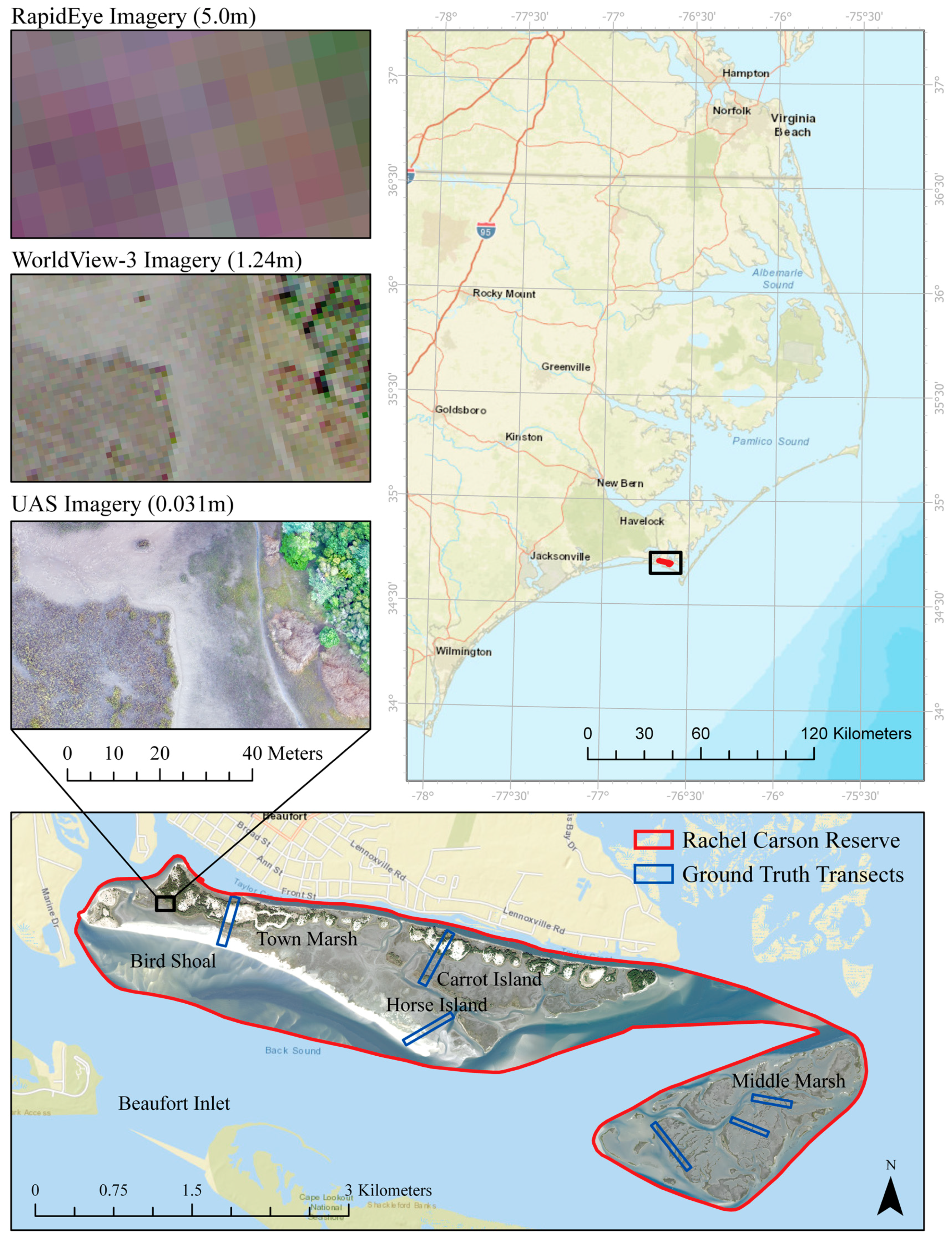
1.4. National Estuarine Research Reserve Program and Rachel Carson Reserve Study Area

In order to combat the degradation of estuaries in the United States over the last century, the Coastal Zone Management Act of 1972 was passed to help conserve these critical systems. This act resulted in the creation of the National Estuarine Research Reserve System (NERRS), a system of reserves meant to foster long-term research and monitoring, education, and stewardship of our estuarine natural resources. A major purpose of these reserves is to provide an undeveloped estuarine testbed, informing local, regional and national management decisions. To accomplish this goal, NERRS has implemented system-wide research and monitoring programs to address various stewardship issues, which includes a Habitat Mapping and Change plan [29]. The Habitat Mapping and Change Technical Committee advises reserves to conduct change analyses at least once every 10 years.
The North Carolina (NC) NERR is one of 28 reserves currently in the NERRS, consisting of several sites along the NC coast that encompass the gamut of physical and ecological environments present in NC’s extensive estuarine network. Centrally located along the coast of NC, the Rachel Carson Reserve (RCR, Figure 1) was created in the 1980s and consists of several fetch-limited barrier islands (Bird Shoal, Town Marsh, Carrot Island, and Horse Island) and a saltmarsh island complex (Middle Marsh). The area is subject to semidiurnal tides with a 0.9 m tidal range, exhibiting extensive saltmarsh platforms, intertidal oyster reefs, shallow seagrass beds, and tidal flats across a low-lying landscape. Vegetated dunes and upland habitats occur along parts of Bird Shoal, Town Marsh, and Carrot Island, which have been historically augmented by dredge spoil. Not only is the RCR ecologically significant [30], as fetch-limited barrier islands [31], the RCR islands help buffer the town of Beaufort from wave energy and storm surge, making their persistence critical for the coastal community.

1.5. Study Objectives

Estuarine wetlands are important for coastal ecology and economies. Improvements in monitoring and mapping estuarine wetlands are needed not only to consistently map the entire reserve system to fulfil the requirements of the NERRS, but also to monitor changes due to human disturbances and sea level rise. Therefore, our objectives are to:
  • Assess the ability of UAS to replace field work for classification algorithm training and validation
  • Compare WorldView-3 and RapidEye for estuarine habitat classification
  • Test the utility of image texture, spectral indices, and data fusion with LiDAR
  • Analyze changes in detailed coastal cover types from 2004 to 2017

2. Materials and Methods

2.1. NERRS Classification Scheme

The NERRS Habitat and Land Cover Classification Scheme (NERRSCS) used in the present study is a framework developed by NOAA and the NERRS to create a consistent scheme for researchers working in the NERRS [32]. This framework combines two well-established schemes, Cowardin et al. [33] and Anderson et al. [34], into a hierarchy with the flexibility to describe broad land cover categories that scales down to dominant vegetation types for each system. The goal of this scheme is to facilitate the classification of high resolution data in estuarine environments and to permit crosswalk with Cowardin’s National Wetlands Classification Standard and the Coastal and Marine Ecological Classification Standard. While no single scheme can serve all remote sensing needs, we employ the NERRS framework in the present study for high resolution classifications in coastal areas that are not purely marine or estuarine as it allows for consistent comparisons across space and time. Table 1 and Table 2 provide details on habitat classes defined in the NERRS classification scheme.

2.2. Remotely Sensed Data

2.2.1. UAS Imagery Collection and Processing

UAS data collection for training the satellite image classifier and validating accuracy of the classification was conducted in August, September and October of 2016, and September of 2017 over parts of the RCR encompassing Bird Shoal, Town Marsh, Carrot Island, and Middle Marsh (Figure S1 and Table S2). Two different UAS were deployed as part of these surveys, a senseFly eBee Plus and a senseFly “standard” eBee. The eBee and eBee plus are small fixed-wing UAS in a push-prop configuration, powered by lithium polymer rechargeable batteries. The eBee Plus was equipped with a senseFly Sensor Optimized for Drone Applications (S.O.D.A.) 20 megapixel camera and a survey-grade RTK GPS capable of 0.03 m of horizontal error (surveys in September of 2017). The standard eBee was equipped with a Canon IXUS 127HS 16.1 megapixel camera, or a Canon S110 12 megapixel camera, as well as a mapping grade GPS capable of 2.5 m of horizontal error (surveys in August, September, and October of 2016). All survey altitudes corresponded to ground sampling distances (GSDs) between 0.025 and 0.031 m, and imagery was collected off-nadir at a 5–7° pitch angle. All flights were automated, with flight plans and image transects generated and executed in the eMotion 3 ground control software programs with 75–85% longitudinal and 75% lateral image overlap.
We processed all UAS imagery with Pix4D Mapper Pro “structure from motion” photogrammetry software to output orthomosaics in the WGS1984 UTM Zone 18 N projection. For all projects, keypoint image scale was set to “Full”, and we enabled the “Alternative” camera calibration setting, which improves calibration accuracy while increasing processing time. Bundle block adjustment results were strong on all projects, with mean reprojection errors between 0.21 and 0.24 pixels.
The five UAS mosaics, covering nearly the entire study area, were co-registered to WV and RE imagery using 50 automatically generated GCPs in each mosaic and manually eliminating incorrect points. Bilinear interpolation was used to resample the imagery and final root mean square error was under one meter for each mosaic, which is well below the geolocation accuracy of the satellite imagery.

2.2.2. WorldView-3 and RapidEye Satellite Imagery

WorldView-3 (WV) imagery is useful for fine-scale habitat mapping, due to its high-spatial and spectral resolution; each image has eight visible and near-infrared bands (1.24-m spatial resolution) and a panchromatic band (0.31-m at nadir) (Table 2). Compared to most multispectral satellites, the addition of four bands (coastal, yellow, red-edge, and near-infrared II) in both WorldView-2 and 3 allow for improved accuracy in mapping wetland vegetation [36,37]. While WorldView-3 has the same spectral bands as WorldView-2, it is in a lower orbit, leading to increased spatial resolution (0.31m panchromatic, 1.24 m multispectral for WV-3 vs. 0.46 m pan, 1.86m multispectral for WV-2). Considering commercially available imagery, WV-3 has the finest spatial resolution in the world. WorldView-3 has a revisit rate of 4.5 days and pointing capability for daily revisits. A WorldView-3 image was acquired from DigitalGlobe [38] on 31 October 2017 at 16:14:35 UTC approximately 1 h after low-tide. The tidal state at the time of image acquisition was +0.22 m above the Mean Lower Low Water (MLLW) tidal datum, defined as the average minimum water level across all tidal days [35]. Harmonic tide predictions were taken from the National Oceanic Atmospheric Administration [35] for the Beaufort, North Carolina reference station (CO-OPS Station ID: 8656483; 34°43.2′N, 76°40.2′W).
RapidEye (RE) has a coarser spatial resolution of five meters with only five bands: blue, green, red, red-edge, and near-infrared (Table 2). However, similarly to WorldView-3, RapidEye has an extra red-edge band, compared to conventional Blue-Green-Red-Near Infrared sensors, that allows for improvements in land cover classification [39] as well as wetland mapping [40]. Despite the reduced spatial and spectral resolution compared to WorldView-3, the revisit time for RapidEye is similar (5.5 days) with pointing capability for daily imaging. Due to five identical RapidEye satellites, their imagery archive is near daily even without pointing. Importantly, for small study regions (<10,000 km2) the archive can be more accessible for researchers and conservation groups through Planet’s Education and Research Program [41]. A RapidEye level 3A image was acquired on 20 July 2017 at 16:04:21 UTC approximately 30 min after low-tide. Level 3A images are already orthorectified and radiometrically/geometrically corrected. At the time of image acquisition, the tidal state for the RapidEye image was at -0.07 m MLLW [35]; a similar tidal state to the WorldView-3 image.

2.2.3. LiDAR derived Digital Elevation Models

LiDAR-derived 1-m digital elevation models (DEMs) were acquired from NOAA [42]. The DEMs were derived using topobathymetric LiDAR flown November 2013 to June 2014, without interpolating across areas missing bathymetric data. DEM elevations were in the ellipsoidal North American Datum 1983, (2011 realization) epoch: 2010 (NAD83). The DEMs had a root mean square error of <1.0 m horizontal accuracy. Vertical accuracy at the 95% confidence interval was 0.112 m in open terrain and 0.215 m consolidated across four land cover types (e.g., open terrain, crops/weeds, forest, and brush/small trees), while not including submerged topography. LiDAR data has proven highly effective in separating estuarine habitat types as an integrated layer in a classification composite [17]. However, we use it here only to delineate the upland and wetland classification types by elevation. This allows areas without recent LiDAR to effectively use our classification approach, without the final elevation class split.

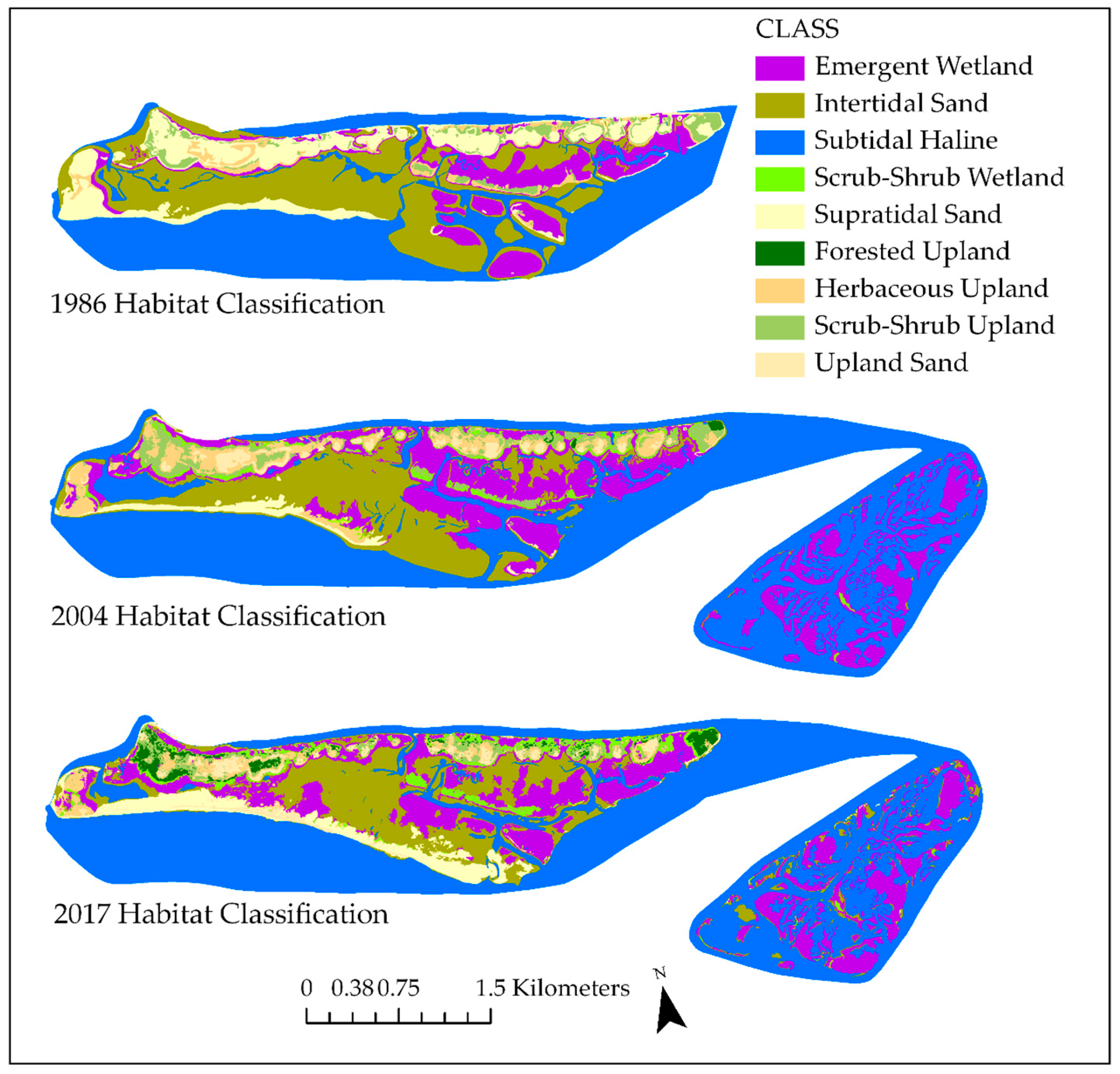
2.2.4. Rachel Carson Reserve Habitat Maps and Change Analysis

A habitat map of the RCR derived from 2004 orthoimagery was obtained from the NC Coastal Reserve and National Estuarine Research Reserve to analyze change across time within the RCR [43]. This imagery was acquired during MLLW at 0.5 m resolution, included RGB and NIR bands, and was classified according to the NERRS Habitat Mapping and Change plan [29]. Their 2004 habitat map was at a similar spatial scale, followed documented NOAA classification procedures, and was classified using the same NERRS Habitat and Land Cover Classification Scheme, and therefore permitted change analysis with our 2017 habitat maps. While specific accuracy was not reported for this map, all federally funded NERRS maps require 68% positional accuracy within 5-m on the ground, 98% producer’s accuracy in delineating wetland areas from non-wetland areas, and 85% attribute accuracy (correct wetland classification) [29]. An additional 1986 habitat map developed for the NCNERRS, which was digitized from aerial imagery flown at low tide, was used for qualitative analysis but not for the quantitative change analysis. All quantitative change analysis was done post-classification and compared total habitat areas. Qualitative change detection analyzed larger general trends, due to the unreported accuracies of the older 1986 habitat map, and thus less validity for analysis of smaller scale changes.

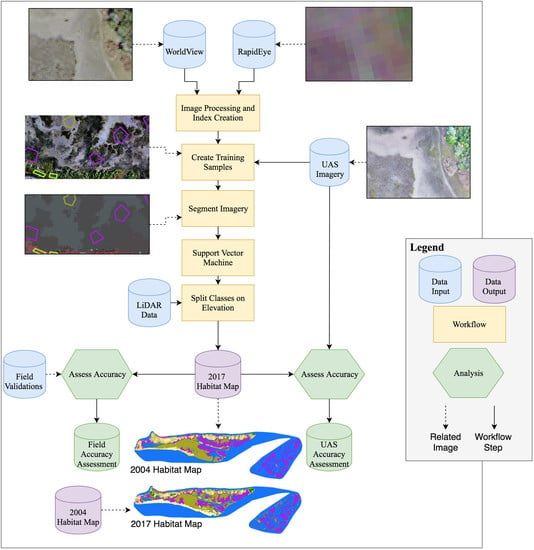
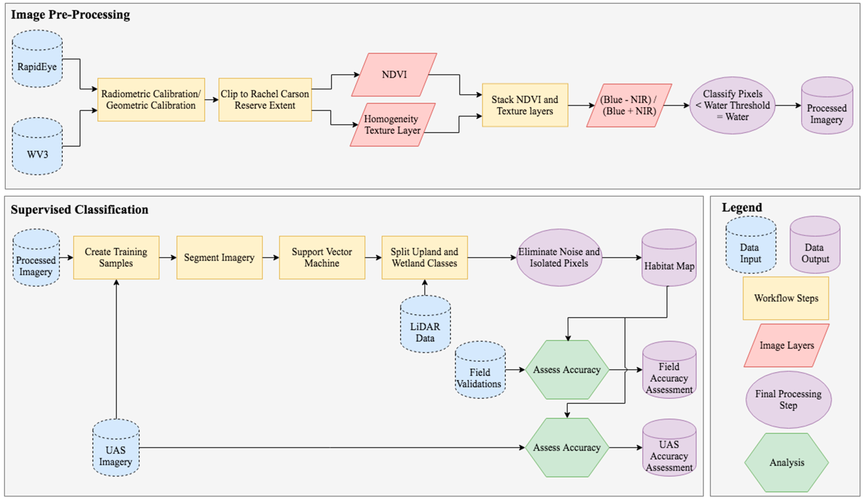
2.3. Image Pre-Processing

Satellite image processing was conducted in ENVI 5.4 (Harris Corporation, Melbourne, FL, USA) and classification was done in ArcGIS Pro 2.0 (ESRI Inc., Redlands, CA, USA) (Figure 2). The images were masked to the RCR, which sped up processing and made NDVI and water thresholds more relevant for our study site. RE and WV imagery come georeferenced but had to be radiometrically calibrated to top of atmosphere reflectance using parameters provided by DigitalGlobe, Inc., (Westminster, CO, USA) and Planet, Inc., (San Francisco, CA, USA). Atmospheric correction was not applied because this study classified a single image in time [44] and previous work has demonstrated only minimal improvement after atmospheric correction for WorldView imagery and other similar multispectral imagery [45]. Pan-sharpening was not applied in the study due to the lack of a panchromatic band on the RapidEye satellite. For each image, a composite was created in addition to the standard RE and WV bands in order to test the impact of including additional indices derived from the original bands on classification accuracy. These composite images included normalized difference vegetation index (NDVI) to emphasize vegetation [46], as suggested by Carle et al. [36] and a homogeneity texture filter using a 3 × 3 kernel (run on NIR1 for WV; NIR for RE) following Lane et al. [47]. Texture layers have been found to help distinguish wetland edges. We eliminated water habitats in our image processing workflow by using a normalized ratio of blue to NIR and eliminating all pixels below a threshold. This threshold was determined by incrementing the value until it included all water pixels in sample polygons drawn to exemplify the multiple Subtidal Haline types (deep, silty, brackish, sandy). Where Rλ is the spectral reflectance of the band centered at λ wavelength, indices and thresholds were:
RE Index: (R475 − R805)/(R475 + R805)  threshold = 0.40,
WV Index: (R427 − R950)/(R427 + R950)  threshold = 0.93.
These threshold values differ due to the increased wavelength of WV’s NIR 2 band (R950) over RE’s NIR 1 band (R805). This process successfully eliminated most water pixels below −0.5 m (NAD83) in the images. This threshold was applied after composite creation to prevent distorting the texture filter with additional edge effects. The final outputs from this image processing include four image products: WV with the standard 8 bands, WV 8 bands + NDVI + texture, RE with the standard 5 bands, and RE 5 band + NDVI + texture.

2.4. Supervised Classification Workflow

Segmentation was performed using segment shape, color, and texture as components of the segmentation. Importance of small spectral differences was emphasized (spectral detail = 20). The same settings were used for both images except for minimum segment size which was 15 pixels for WV imagery and 10 for RE imagery due to the increased size of RE pixels. Training samples were created by manually drawing polygons representing each habitat class using the UAS mosaics as a reference (Figure 3). These UAS-derived training polygons were overlaid on segments from the segmentation process and the segment with the greatest area of overlap with each UAS-derived training polygon was identified. These identified segments were then used as training inputs for each classification (Figure 2). This allowed the same training areas to be identified for both the RE and WV-3 imagery even though segmentation was performed separately for each imagery type. Training polygons included between 5000–6000 m2 of each class in order to accurately capture spectral variation (Figure 4) and prevent training data imbalance between classes [48].
Following segmentation, a Support Vector Machine (SVM) was used to classify all four image products. SVMs have been shown to handle large images, are less vulnerable to image noise, do not require a normal distribution of reflectance values, and provide classification results on par with other top algorithms [49]. SVMs are commonly used for classification applications, our contribution here lies in the use of added decision nodes for water classification, testing of image texture and NDVI, and UAS for SVM training and validation. The SVM output was split into Upland and Wetland classes using the LiDAR DEM acquired from NOAA, based on the tidal range of this region. Areas 0.9 m above MLLW were assigned to the Upland class [35] following the definition of these two classes (Table 1). Very high-resolution satellites often have many spectrally mixed pixels and segments, leading to a blur between land cover types that, when averaged together, may be incorrect. These isolated pixel groups (n < 40 for WV, n < 6 for RE) were removed, and re-classified using a majority filter in the final classification map.

2.5. Accuracy Assessment

For both UAS and field-based sample points, stratified sampling was used to assess accuracy of each class. Strata for both UAS and field points were generated from one map (WV 8-band classification). Following Stehman [50] we generated error matrices, user’s (commission error), producer’s (omission error), and overall accuracy, while accounting for differences in strata and map classes. These formulas differ from standard accuracy assessment methods, because they account for strata that have different overall areas within the study site, by weighting accuracy based on the area in each strata. An additional assessment was done by applying the UAS assessment method to the points used for the field validation in order to directly compare the results from both methods.

2.5.1. UAS Assessment

We generated sets of 50 randomly distributed stratified sample points [51] across the nine habitat classes throughout our full study site. This was done using the WV 8-band classification to generate a total of 450 assessment points. These points were overlaid on the UAS mosaics (Figure S1), which had been co-registered to the WV and RE imagery, and classes for each point were visually determined from the UAS imagery. All visual validation was done by the same individual to remain consistent.

2.5.2. Field Assessment

Six linear transects were selected to ensure full coverage of habitat classes denoted in the full study area. Validation points were created by generating 30 randomly distributed stratified sample points across the nine habitat classes within these transect areas, using the WV 8-band classification to define the strata. To minimize the risk of potential errors from GPS and imagery georectification, a −3m buffer was put on each habitat class in the image, eliminating border areas where GPS error could have located a point in a separate class, and points were generated in the remaining habitat area only. Additionally, points were created with a minimum distance of 5 m between to accommodate for the resolution of the RE pixel size. With these constraints in place, a total of 214 total sampling points were created.
Ground observations of habitat classes were taken in February 2018. A Trimble Juno 3B GPS unit was used to locate the approximate location of the validation points. Once the approximate site was reached, the validation point location was taken using a sub-meter accuracy GPS unit (Emlid Reach RS RTK) and the observed habitat type at that validation point was recorded. Classification of the observed habitat type in the field was determined by one individual for all validation points to ensure consistency. The size of a WV pixel was used for determining habitat class. Field-collected validation points were differentially corrected from the local GNSS virtual base station network.
While not practical in our field validation to do truly random sampling throughout the study site due to time constraints, the possibility of transects being in deep water, and a desired balance between classes, transects were otherwise chosen to best ensure representativeness. Where possible we followed best practices presented in Olofsson et al. [52]: UAS stratified sample points were chosen at random throughout the entire study site, assessment units were chosen to match input and reference data, and the accuracy assessment accounted for our stratified sampling approach.

3. Results

This section may be divided by subheadings. It should provide a concise and precise description of the experimental results, their interpretation as well as the experimental conclusions that can be drawn.

3.1. Estuarine Habitat Mapping

Our final maps had area weighted accuracies ranging from 79% field/83% UAS to 93% field/93% UAS (Table 3). The standard 8-Band WorldView-3 image realized the best overall accuracy at 93% field and 93% UAS. Notably, the addition of NDVI and image texture did not increase the accuracy of the WorldView-3 classification but did marginally increase the RapidEye classification accuracy in both UAS and field assessments (Figure 5). Across all final classifications there was a consistent underestimation of Emergent Wetland. The addition of NDVI and texture to WorldView-3 did appear to increase the discrimination of the segmentation between classes, but increased confusion of the final classification between the Scrub-Shrub and Emergent Wetland Classes as well as Intertidal Sand and Subtidal Haline. On the RapidEye platform, the addition of NDVI and texture improved differentiation between Scrub-Shrub and Forest but otherwise overall accuracy was not markedly different with or without NDVI and texture (Table S1).

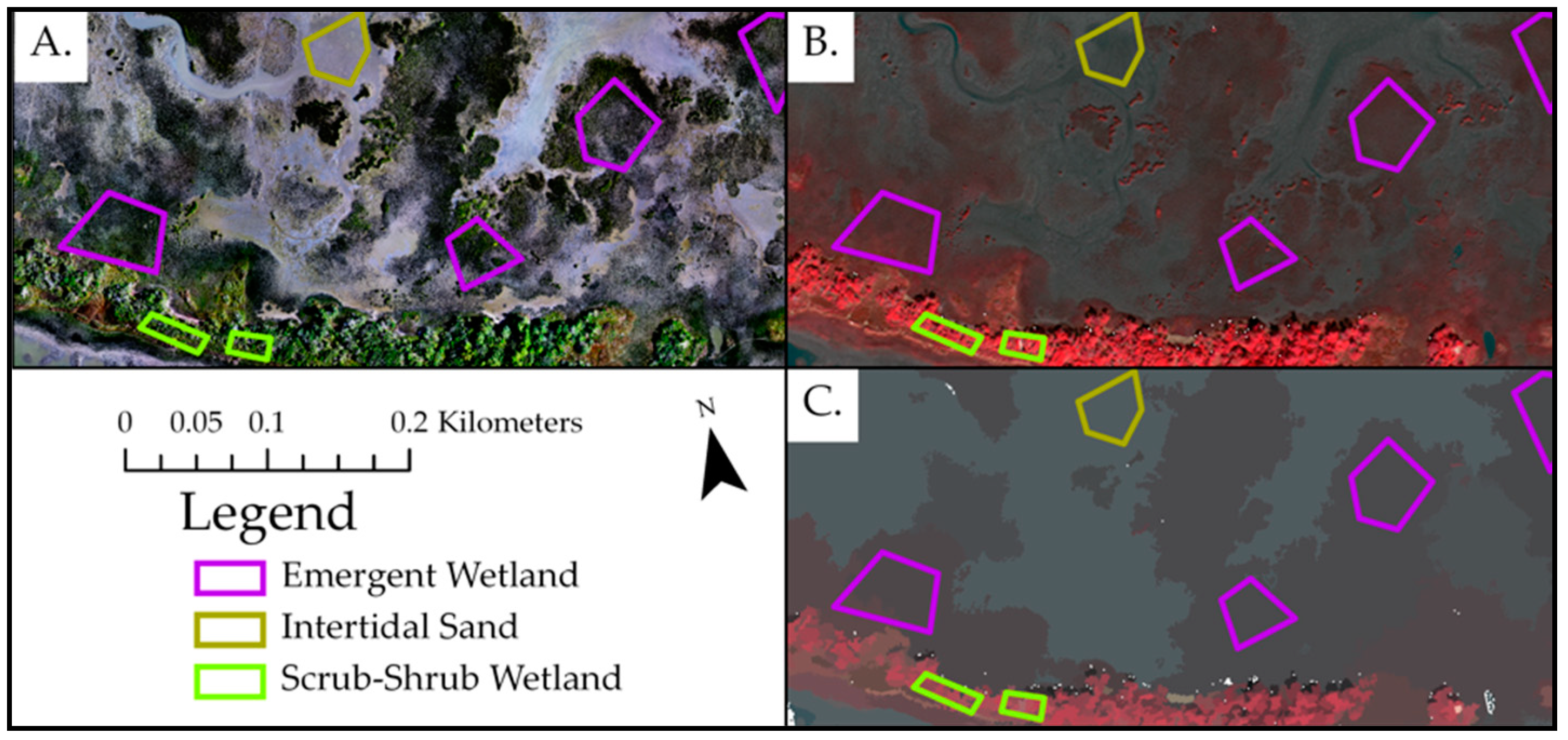
3.1.1. UAS vs. Field Validation

The direct comparison between UAS and field assessment methods had an overall agreement of 96% with minimal variation from that accuracy among classes (Table 4). For the WorldView-3 classifications, the UAS and field validation results correspond well to each other (Figure 5, Table 5 and Table 6). On the RE platform there is a nontrivial difference in field and UAS assessment results for some classes (Table S1). This appears to be from a lack of field test points, or a concentration of field test points in a small misclassified area of a transect, rather than a true divergence in results between UAS and field-based methods.

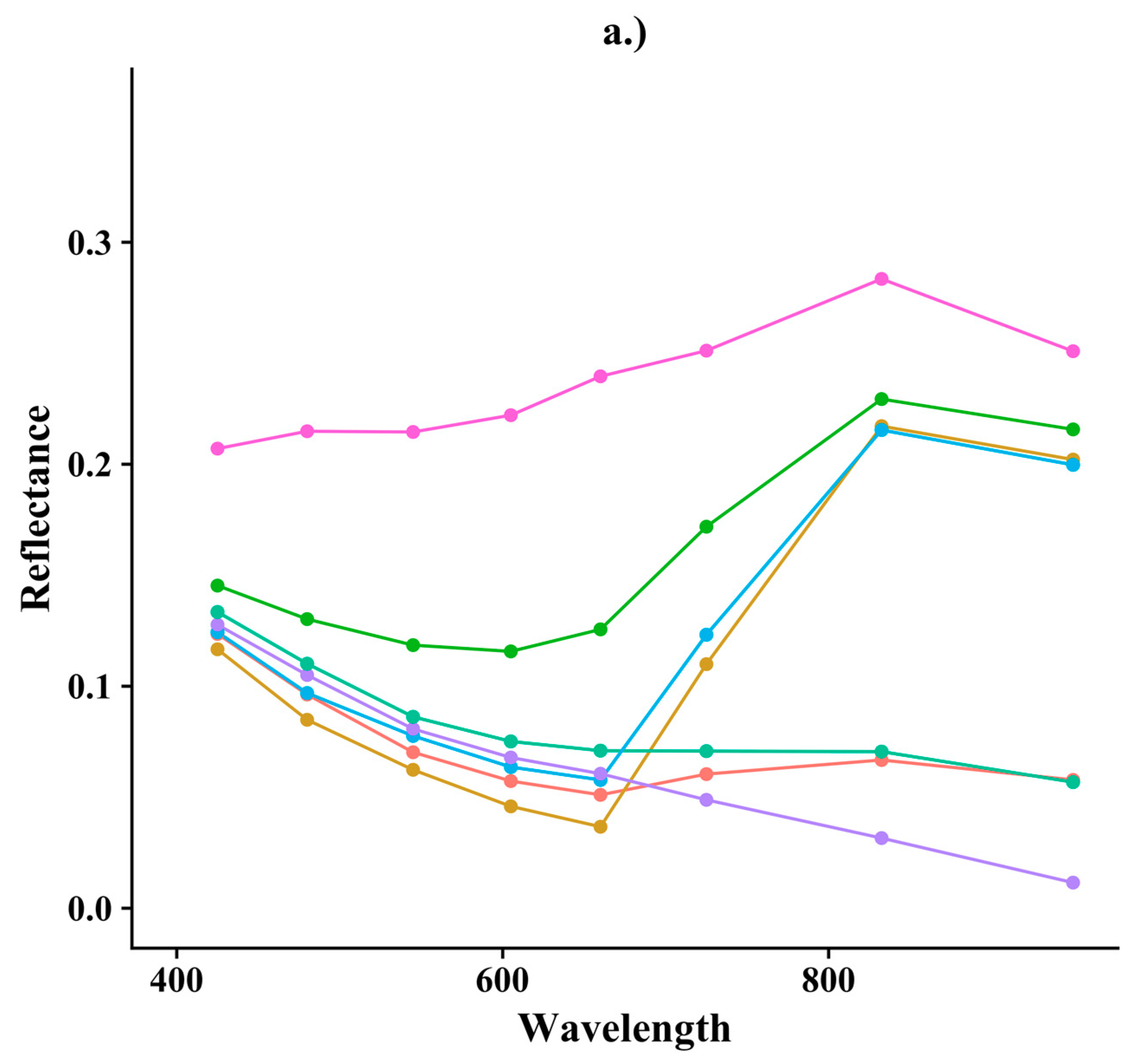
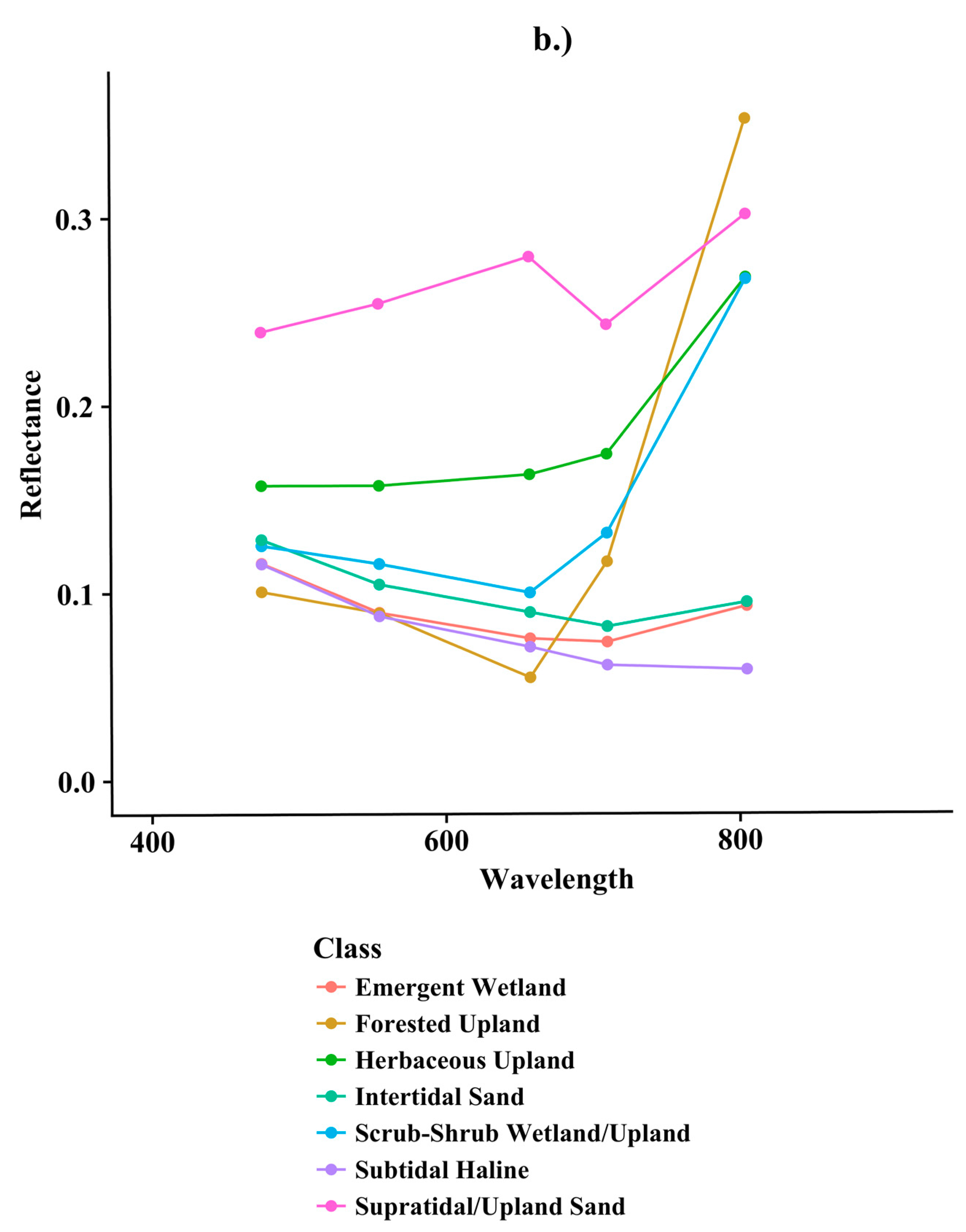
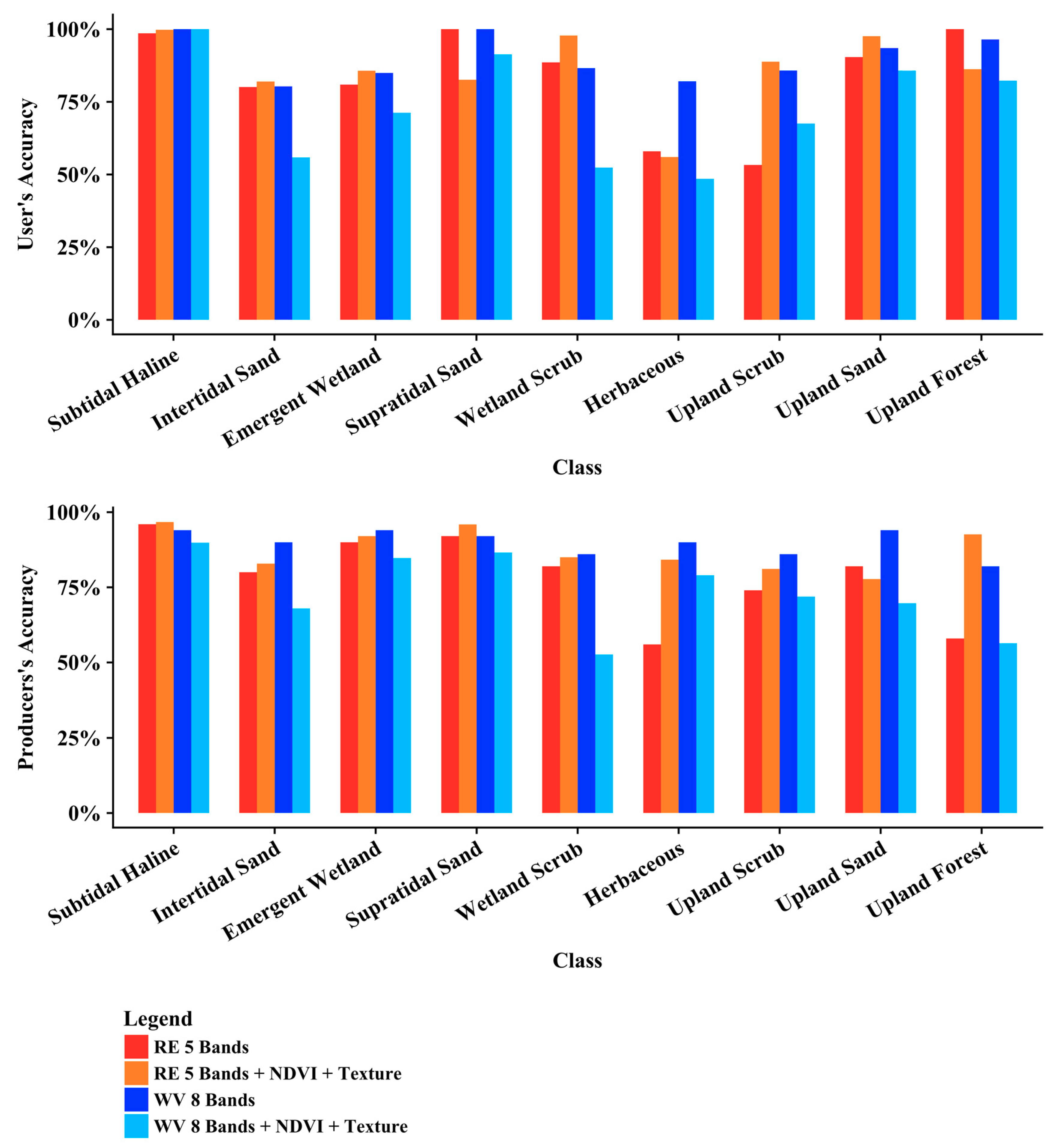
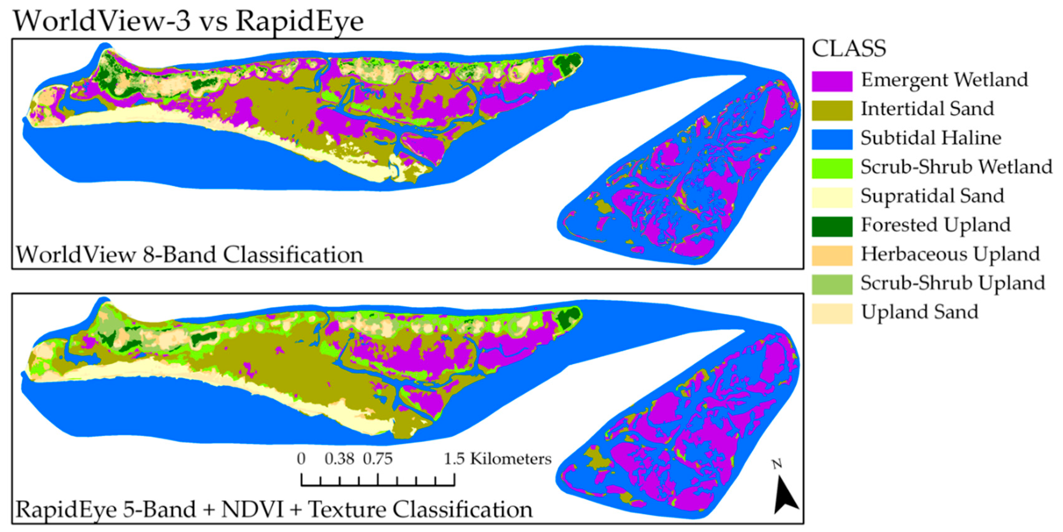
3.1.2. WorldView-3 vs. RapidEye

Results from both WV and RE are promising for their ability to accurately map wetland habitats (Figure 5 and Figure 6). Given that some habitat patches within the study area are <25 m2 (the area of a RE pixel) it was assumed that RE would have trouble distinguishing these features. This was particularly evident in the over prediction of scrub-shrub in RE imagery and can be seen in the training sample spectral signatures where there is more noise and mixing in the classes evidenced by the dip in the Supratidal Sand class on the red edge band, suggesting some mixing with slightly vegetated pixels. These partially mixed pixels were overpowered by the scrub-shrub class and were actually more often herbaceous, emergent wetland, or sand. Results show classifier confusion between scrub-shrub and herbaceous that could not be differentiated by RE, but could with WV, likely due to increased spatial resolution rather than spectral differentiation (Table S1). Other than this difficulty differentiating the herbaceous class on RE, RE and WV had similar results across the other classes. Both had difficulty separating emergent wetland from intertidal sand and scrub-shrub and high accuracy for most other classes.

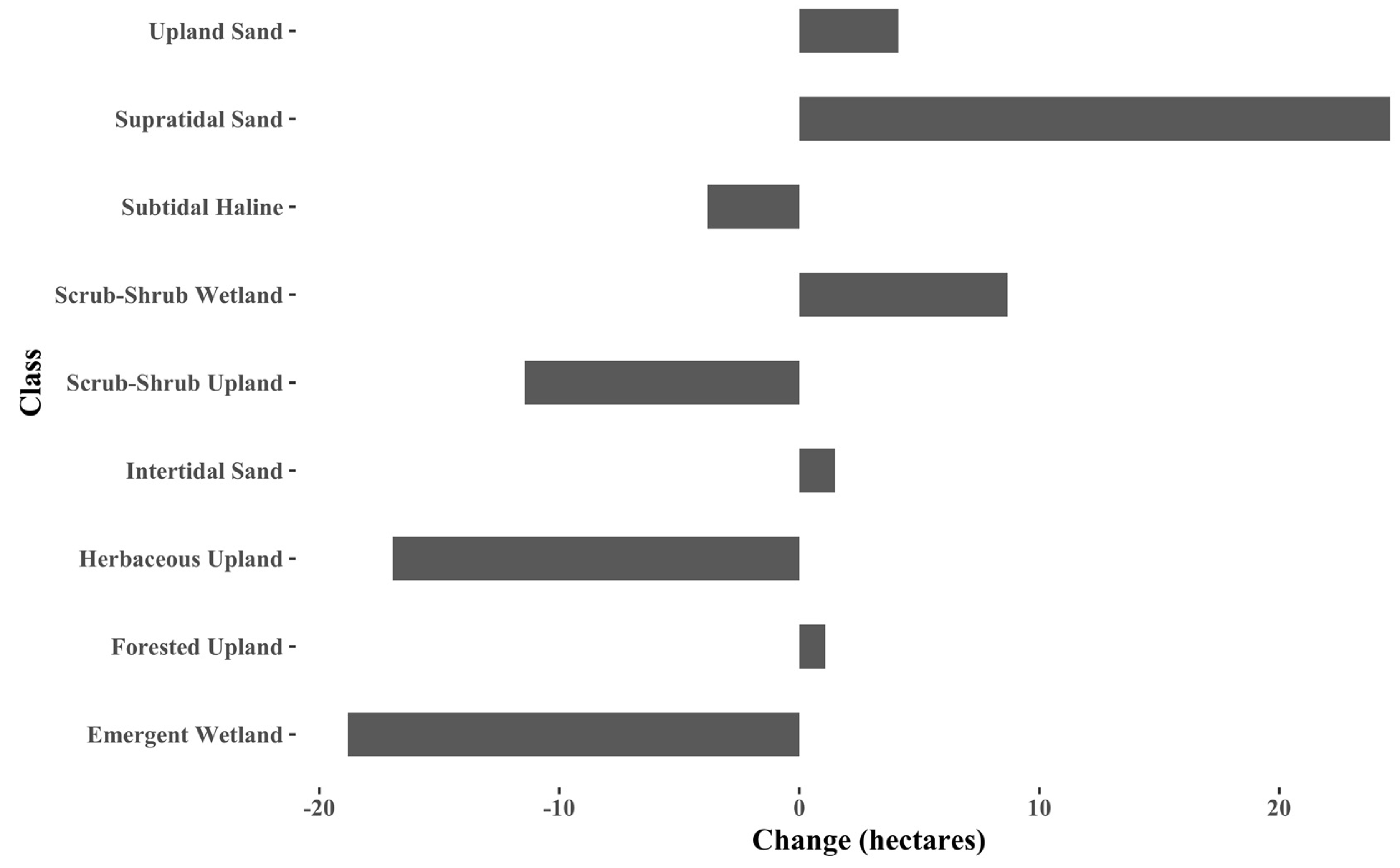
3.2. Change Analysis with 2017 RCR Map

The greatest change in the RCR from 2004 to 2017 occurred in the supratidal sand class, which expanded in coverage across the Bird Shoal shoreline (Figure 7). While a less pronounced change, a relatively large increase in upland forest habitat corresponded with decreases in upland scrub-shrub and upland herbaceous habitats. Total areal changes to emergent wetlands and intertidal sands were small, but patterns of change with these two cover types vary across the RCR, indicating regional expansion and loss of wetlands over the past three decades (Figure 8). Middle Marsh experienced a 9% loss of emergent wetlands, with gains in upland scrub-shrub and intertidal sand.

4. Discussion

4.1. UAS and Field Work for Validation

Considering the similarity in accuracy between UAS and field-based assessments, our conclusion is strongly in favor of validation with UAS where feasible. Primarily, this is due to the increased ability to sample validation points across a larger proportion of the study site, while requiring less time and less intrusion on the study area. For our study, using conventional field-based methods required two 10-h days for three individuals to validate six small transects (214 validation points in 30 h across 186,000 m2) and UAS-based methods required five hours of mission planning, five two-hour expeditions of two individuals, and five hours of post-flight analysis to map the entire study area (450 validation points in 15 h across 4,325,000 m2).
While startup costs of pilot training and platform acquisition may be relatively high, the benefits appear to outweigh the costs in most applications. UAS imagery can be taken much more rapidly than a comparable number of field points, meaning smaller windows in acceptable weather, season, and tidal condition are sufficient for data collection. This should allow for validation data acquisition to be closer in time to the satellite imagery. Aerial surveys also do not require a field team to trek through a fragile wetland environment that may itself influence the study site over time. Moreover, aerial imagery allows for a direct comparison to various satellite pixel sizes, which is more flexible and accurate than bringing quadrats into the field and looking at them from the ground. UAS imagery, combined with properly georectified structure from motion processing, permits geolocation errors <0.05 m (Seymour et al., 2017a). Co-registering satellite imagery to georectified UAS imagery can result in <1 m geolocation error even over large study sites, compared to typical 3–5 m satellite image geolocation error plus any GPS uncertainty in the field. Given that satellites like WorldView-3 can capture features as small as a single tree, or a tendril of emergent wetland, this precision in geolocation is necessary for accurate training and assessment of very high resolution imagery. Tidal rectification of satellite imagery with UAS is straightforward, as typically the tidal state does not change substantially within the duration of a single flight and can be matched easily. Conversely, it is not typically feasible to constrain traditional in-situ fieldwork to a precise tidal period, especially over large study areas. An additional benefit from UAS, though not done in this study, is to include UAS-based Digital Surface Models (DSMs) to add to training and validation accuracy by incorporating elevation into the workflow [18].
In addition to startup and training costs, there are a few limitations with UAS that should be considered. For example, shadows and glare can prevent an analyst from visually determining water depth or vegetation type; however, appropriate flight timing can limit this issue. Typically, early morning and late afternoon provide minimum glare due to the low sun angle, which is ideal for flights over water and other reflective surfaces. Mid-day flights are ideal in areas with high relief and tall vegetation for minimal shadows. Wind and weather can also prevent smaller platforms from safely operating even if other conditions are ideal and add to glare on water. Early morning flights often mitigate wind issues in coastal areas. Small differences in our UAS and field validation results can be attributed to tidal offset, georeferencing error, vegetation change from August 2016 to February 2018, and the limited number of field points that were taken due to the high time and resource requirements of field validation. In addition to these logistical challenges, sole reliance on UAS-based methods may lead to further issues, such as remote pilots lacking basic knowledge about the ecosystem that will help better design classification systems and interpret classification issues.
The strongest argument for UAS-based training and validation is that, within a fixed budget, it allows much larger training and testing sample sizes. If we had determined it was worthwhile we could have used 2–3 times as many UAS-based training and testing points for this study, or covered much more area in flights, with only marginal increases in cost and time. Increasing the field-based sample sizes by two times would have been prohibitive, as it would have been a proportional increase in cost and time. New classification techniques are being developed, including deep learning methods, and additional satellite constellations are being launched. In the context of these new classifiers and satellite imagery, highly accurate testing and training datasets covering large areas will be critical for monitoring ecosystems and change across time. We suggest UAS as a critical component of this process moving forward.

4.2. WV3 and RE Classifications

The present study adds to a growing body of work demonstrating WorldView-3’s mapping abilities and is one of the first to compare WV and RE in an estuarine environment. Different spatial scales for segmentation had a considerable impact on the accuracy of the final habitat class map, as has also been found in previous object-based wetland mapping projects [49]. Few previous studies provide a reason for their segmentation level, despite being a considerable factor in the final classification output. The level used in this study was determined iteratively with a large number of test sites through the study area visually examined at each segmentation level. Although not necessary in our study, other mapping projects with different landscape features often require multiple segmentation levels to create separate classification maps each designed for delineating a specific habitat class that could then be merged into a final product.
Given that the accuracy for both platforms was above 85% (UAS-based), the tradeoffs between them cannot be defined simply by overall accuracy. Many ecologically important features within wetlands are smaller than 5 m, so understanding change at that scale may require WV or aerial imagery. In many cases the added spatial and spectral resolution makes WV a clear choice, especially if it is affordable and available at the appropriate acquisition time. Though WorldView-3 has an orbital revisit rate of 4.5 days, in practice imagery is considerably more limited for environmental monitoring, and satellite tasking is beyond the budget of most projects. Thus, the added temporal availability, better access for researchers, and decade-deep imagery archive make RE an enticing choice for many applications.
In wetland mapping, tidal and seasonal matches are critical for accurate change analysis. The higher revisit rate of RE captures ideal seasons and tides more frequently [53]. This multitemporal stack also helps mitigate the impact of clouds and allows imagery acquisition more immediately after storm or pollution events. These tradeoffs need to be understood as new commercial constellations by companies such as Planet and BlackSky arise; these additional satellites will add more options for high revisit rates in the future, though potentially at lower spatial and spectral resolution, and without the benefit of long historical archives.

4.3. Image Layers and Thresholding

The contribution of NDVI and texture to class differentiation on RE is similar to what previous studies have found with just the addition of NDVI on RE [54]. The decrease in accuracy on WV with these added layers leads to additional questions and could have been caused by the SVM overfitting the training samples, differences in training and validation samples, or too much noise in the additional layers. A growing body of work suggests dimensionality reduction may be as effective as adding data dimensions in some applications [55,56,57]. Our results from analyzing the contribution of these layers promote the claim that one must consider the specific platform, and its spectral and spatial characteristics, to decide whether additional indices or texture features will add to the prediction power of a multispectral image. As deep learning classifiers find their way into the mainstream, where handcrafted layers are not typically necessary, these added dimensions may fall out of favor.
Water habitats within this estuarine environment are highly complex; for example, some areas exhibit clear deep water and low reflectance values, while other water pixels have high NDVI, turbidity, and textured bottom types (oyster shells, debris, etc.). This drives a high amount of spectral variation in the subtidal haline class, causing confusion for classification algorithms. This thresholding step eliminated that confusion by successfully delineating water from other classes and has the potential for applicability across environments.

4.4. Conservation Implications

Much of the land cover change occurring in the RCR over the past few decades is due to successional processes. However, these maps show the result of geophysical drivers that are continuing to shape Bird Shoal as well as the potential impact of sea-level rise (SLR) on saltmarshes in this area. Succession is best evidenced by the conversion of herbaceous and scrub-shrub habitat to forest, and the colonization of intertidal sandflats by saltmarsh vegetation. Examination of the supratidal sand component reveals a long-term pattern of sediment redistribution within the RCR. For the past decade, the supratidal component of Bird Shoal has been steadily growing as nearby Beaufort Inlet has been widening. Prevailing winds occur from the southwest, and several tropical cyclones have directly impacted the study area during this time, including Hurricanes Ophelia, Irene, Arthur, and Matthew, which together appear to have resulted in overwash and longshore delivery of sediments, extending the island to the east. Because of the sheltered nature of fetch-limited barrier islands, storm overwash has significantly reduced return energy, resulting in primarily landward movement of the beach [58], and nearshore wave refraction is decreased, yielding greater alongshore transport of sediment [31]. Overwash and aeolian transport across sparsely vegetated areas have delivered sediment to the low relief area between Bird Shoal and Town Marsh, increasing the elevation and providing suitable habitat for saltmarsh vegetation to colonize [59,60]. Thus, we see substantial increases of intertidal emergent wetland habitat in the western third of the RCR. This expansion of Bird Shoal has also encroached on other areas of the RCR, with the island migration rolling over emergent wetlands and now bleeding into Horse Island. With SLR, the migration of Bird Shoal will likely continue, eventually overtaking Horse Island and narrowing the low-lying intertidal wetlands between the outer shoreline and the dredge spoil mounds on the north side of the RCR. The speed at which this migration occurs will depend on the island’s recovery, the continued impact of Beaufort Inlet dynamics, future storm activity, and the rate of local SLR. Changes in the extent of different habitat types may have implications for the management of living resources within the RCR. The RCR represents important seasonal habitat for several endangered species of plants and animals [61], and is also home to a stable population of feral horses that exert both direct and indirect effects on the local estuarine ecosystem [62]. As these habitats evolve, conflicts amongst management priorities may emerge [63], and the workflows provided in the present study provide an initial framework for RCR managers to efficiently monitor habitat change and plan for such conflicts.
Island movement within the RCR in response to storms and inlet changes is likely compounded by the occurrence of higher water levels within the past decade. Interaction of the North Atlantic Oscillation and the El Niño Southern Oscillation have caused hotspots in local SLR along the US East Coast since 2011 [64], and the region has experienced periods of frequent sea-level anomalies [65,66]. Higher water levels can result in more rapid sediment erosion or accretion depending on the forcing patterns [67] and whether the shoreline has already been compromised by a recent storm [66]. Increased water levels may be contributing to the loss of emergent wetlands in the eastern portions of the RCR (Carrot Island, Horse Island, and Middle Marsh), as increased inundation leads to greater marsh bank erosion and saltmarsh die off in the lower intertidal [68,69,70]. Being linked to atmospheric-oceanic cycles, the area will experience periods with lower rates of SLR, which may allow some recovery of emergent wetlands. However, this region does not have high suspended sediment loads to support greater marsh accretion rates [4], and with continued SLR many of these lost emergent wetland areas may not be recoverable.
The use of high resolution satellite imagery coupled with UAS-based image training has allowed us to effectively compare land cover changes within the NCNERR, given the availability of historical habitat mapping data. These maps through time have provided a window into natural and human impacts to the RCR, and there is growing potential to implement these methods on broader scales, encompassing more environments with the increasing accessibility of both satellite and UAS technology. Furthermore, the existing archive of RE/WV2/WV3 imagery enables comparisons using the same spectral bands as far back as 2010, providing a vast imagery dataset that is high in both spatial and temporal resolution.

4.5. Continuing Difficulties and Future Work

While testing these methods in the coastal environment, we have recognized several challenges that should be considered moving forward. Given that intertidal sand, scrub-shrub wetland, and emergent wetland do mix on the ground, with soft transitions between classes, a fuzzy accuracy assessment may be appropriate in future studies to fully capture the accuracy of classification algorithms [71]. It is up for debate whether using pixels or segments is more appropriate for assessing the accuracy of object-based classifications. We suggest future studies build on our work by using the segment level, area-based assessment methods suggested by Ma et al. [72]; implementation of this segment-level assessment method using UAS would be considerably easier compared to a field-based approach. Integrating this with a fuzzy accuracy assessment may become the standard for future object-based classifications in complex environments such as estuarine habitats, where interfaces among classes are often difficult to differentiate. However, when using UAS for training and validation data, some level of familiarization of the landscape will still be required, perhaps facilitated through direct coordination with a local expert having personal knowledge of the study area.

5. Conclusions

This study provides a detailed example for future integrations of UAS sampling and satellite imagery in the study of coastal landscape changes. When deciding between satellite imagery, we suggest considering the spatial extent of a study site, the finest features, spectral similarity of classes, timing specificity requirements, and total budget. For example, the finer resolution of WV imagery may be more useful when classification subjects are smaller and similar in spectral signatures to nearby environments, but the frequency of RE imagery could be more beneficial for capturing temporally short-term changes (e.g., storm impacts). Sensor selection should then drive additional indices and image layers, with higher dimensional multispectral datasets not always needing additional layers, as in our study. When evaluating UAS versus field-based validation, we find that, across the board, increased numbers of sample points over a larger area augment the quality and reliability of the final accuracy results. UAS-based accuracy assessment allows for a greater number of validation points to be collected with marginal impact to processing time, permits field work to be conducted within rapid collection windows, and leaves a minimal environmental footprint.

Supplementary Materials

The following are available online at https://0-www-mdpi-com.brum.beds.ac.uk/2072-4292/10/8/1257/s1, Table S1: Full confusion matrices for unoccupied aircraft system and field-based validations. Figure S1: Unoccupied Aircraft System (UAS) imagery of the Rachel Carson Reserve. Top shows the outline of the Reserve with all mosaics, UAS validation points, and a base map of satellite imagery for reference. Bottom shows just the outline of the Reserve and the UAS mosaics labeled by flight number. Note: all validation points not covered by UAS imagery were clear subtidal haline points and thus did not need additional resolution beyond that of the satellite imagery to determine class. Table S2: Flight details for unoccupied aircraft system (UAS) imagery of the Rachel Carson Reserve.

Author Contributions

Conceptualization, J.J.S., A.M.S., D.W.J., and P.C.G.; Methodology, J.T.R., S.K.P., A.C.S., J.J.S., and P.C.G.; Software, A.C.S. and P.C.G.; Data Curation: J.T.R., S.K.P., A.C.S., P.C.G.; Investigation, J.T.R., S.K.P., D.W.J., and P.C.G.; Validation, J.T.R., S.K.P., and P.C.G.; Formal Analysis, J.T.R., S.K.P., A.M.S., and P.C.G.; Funding Acquisition, J.T.R. and S.K.P.; Writing-Original Draft Preparation, P.C.G., J.T.R., S.K.P., A.C.S., A.M.S., J.J.S., D.W.J.; Writing-Review & Editing, P.C.G., J.T.R, S.K.P., A.C.S., A.M.S., J.J.S., D.W.J.

Funding

This research was supported by the North Carolina Sea and Space Grant Graduate Fellowship (Grant # 2017-R/MG-1710) as well as the North Carolina Coastal Recreational Fishing License Grants Program (Marine Resources Fund, Grant # 2017-H-068).

Acknowledgments

We thank Brandon Puckett and Rodney Guajardo of the North Carolina Coastal Reserve for sharing their 2004 Habitat Map of the Rachel Carson Reserve and GIS knowledge. We thank Anna Windle for constructive feedback through this research project and Everette Newton for imagery and insight into the Reserve’s structure. We also appreciate the satellite imagery generously provided for this project from the DigitalGlobe Foundation and Planet Inc.

Conflicts of Interest

The authors declare no conflicts of interest.

References

  1. Barbier, E.B.; Hacker, S.D.; Kennedy, C.; Kock, E.W.; Stier, A.C.; Brian, S.R. The value of estuarine and coastal ecosystem services. Ecol. Monogr. 2011, 81, 169–193. [Google Scholar] [CrossRef] [Green Version]
  2. Kirwan, M.L.; Temmerman, S.; Skeehan, E.E.; Guntenspergen, G.R.; Fagherazzi, S. Overestimation of marsh vulnerability to sea level rise. Nat. Climat. Change. 2016, 6, 253–260. [Google Scholar] [CrossRef]
  3. Spalding, M.D.; Ruffo, S.; Lacambra, C.; Meliane, I.; Hale, L.Z.; Shepard, C.C.; et al. The role of ecosystems in coastal protection: Adapting to climate change and coastal hazards. Ocean Coast Manag. 2014, 90, 50–57. [Google Scholar] [CrossRef]
  4. Kirwan, M.L.; Guntenspergen, G.R.; D’Alpaos, A.; Morris, J.T.; Mudd, S.M.; Temmerman, S. Limits on the adaptability of coastal marshes to rising sea level. Geophys Res Lett. 2010, 37, 1–5. [Google Scholar] [CrossRef]
  5. Mitchell, S.B.; Jennerjahn, T.C.; Vizzini, S.; Zhang, W. Changes to processes in estuaries and coastal waters due to intense multiple pressures—An introduction and synthesis. Estuar. Coast Shelf Sci. 2015, 156, 1–6. [Google Scholar] [CrossRef]
  6. Raposa, K.B.; Weber, R.L.J.; Ekberg, M.C.; Ferguson, W. Vegetation Dynamics in Rhode Island Salt Marshes During a Period of Accelerating Sea Level Rise and Extreme Sea Level Events. Estuar. Coast . 2017, 40, 640–650. [Google Scholar] [CrossRef]
  7. Klemas, V. Remote Sensing Techniques for Studying Coastal Ecosystems: An Overview. J. Coast Res. 2011, 27, 2–17. [Google Scholar] [CrossRef] [Green Version]
  8. Adam, E.; Mutanga, O.; Rugege, D. Multispectral and hyperspectral remote sensing for identification and mapping of wetland vegetation: A review. Wetl. Ecol. Manag. 2010, 18, 281–296. [Google Scholar] [CrossRef]
  9. Dronova, I. Object-Based Image Analysis in Wetland Research: A Review. Remote Sens. 2015, 7, 6380–6413. [Google Scholar] [CrossRef] [Green Version]
  10. McCarthy, M.; Halls, J. Habitat Mapping and Change Assessment of Coastal Environments: An Examination of WorldView-2, QuickBird, and IKONOS Satellite Imagery and Airborne LiDAR for Mapping Barrier Island Habitats. ISPRS Int. J. Geo-Inf. 2014, 3, 297–325. [Google Scholar] [CrossRef] [Green Version]
  11. Le Bris, A.; Rosa, P.; Lerouxel, A.; Cognie, B.; Gernez, P.; Launeau, P.; Robin, M.; Barillé, L. Hyperspectral remote sensing of wild oyster reefs. Estuar. Coast Shelf Sci. 2016, 172, 1–12. [Google Scholar] [CrossRef]
  12. Heenkenda, M.K.; Joyce, K.E.; Maier, S.W.; Bartolo, R. Mangrove species identification: Comparing WorldView-2 with aerial photographs. Remote Sens. 2014, 6, 6064–6088. [Google Scholar] [CrossRef]
  13. Laba, M.; Blair, B.; Downs, R.; Monger, B.; Philpot, W.; Smith, S.; Sullivan, P.; Baveye, P.C. Use of textural measurements to map invasive wetland plants in the Hudson River National Estuarine Research Reserve with IKONOS satellite imagery. Remote Sens. Environ. 2010, 114, 876–886. [Google Scholar] [CrossRef]
  14. Henderson, F.M.; Lewis, A.J. Radar detection of wetland ecosystems: A review. Int. J. Remote Sens. 2008, 29, 5809–5835. [Google Scholar] [CrossRef]
  15. Guo, M.; Li, J.; Sheng, C.; Xu, J.; Wu, L. A review of wetland remote sensing. Sensors 2017, 17, 777. [Google Scholar] [CrossRef] [PubMed]
  16. Joshi, N.; Baumann, M.; Ehammer, A.; Fensholt, R.; Grogan, K.; Hostert, P.; Jepsen, M.R.; Kuemmerle, T.; Meyfroidt, P.; Mitchard, E.T.A.; et al. A review of the application of optical and radar remote sensing data fusion to land use mapping and monitoring. Remote Sens. 2016, 8, 70. [Google Scholar] [CrossRef]
  17. Halls, J.; Costin, K. Submerged and emergent land cover and bathymetric mapping of estuarine habitats using worldView-2 and liDAR imagery. Remote Sens. 2016, 8, 718. [Google Scholar] [CrossRef]
  18. Kalacska, M.; Chmura, G.L.; Lucanus, O.; Bérubé, D.; Arroyo-Mora, J.P. Structure from motion will revolutionize analyses of tidal wetland landscapes. Remote Sens. Environ. 2017, 199, 14–24. [Google Scholar] [CrossRef]
  19. Wan, H.; Wang, Q.; Jiang, D.; Fu, J.; Yang, Y.; Liu, X. Monitoring the invasion of Spartina alterniflora using very high resolution unmanned aerial vehicle imagery in Beihai, Guangxi (China). Sci. World J. 2014, 2014, 14–16. [Google Scholar] [CrossRef] [PubMed]
  20. Durban, J.W.; Fearnbach, H.; Perryman, W.L.; Leroi, D.J. Photogrammetry of killer whales using a small hexacopter launched at sea. J. Unmanned Veh. Syst. 2015, 3, 1–5. [Google Scholar] [CrossRef]
  21. Seymour, A.C.; Dale, J.; Hammill, M.; Halpin, P.N.; Johnston, D.W. Automated detection and enumeration of marine wildlife using unmanned aircraft systems (UAS) and thermal imagery. Sci. Rep. 2017, 7, 45127. [Google Scholar] [CrossRef] [PubMed] [Green Version]
  22. Sykora-Bodie, S.T.; Bezy, V.; Johnston, D.W.; Newton, E.; Lohmann, K.J. Quantifying Nearshore Sea Turtle Densities: Applications of Unmanned Aerial Systems for Population Assessments. Sci. Rep. 2017, 7. [Google Scholar] [CrossRef] [PubMed] [Green Version]
  23. Mancini, F.; Dubbini, M.; Gattelli, M.; Stecchi, F.; Fabbri, S.; Gabbianelli, G. Using unmanned aerial vehicles (UAV) for high-resolution reconstruction of topography: The structure from motion approach on coastal environments. Remote Sens. 2013, 5, 6880–6898. [Google Scholar] [CrossRef] [Green Version]
  24. Seymour, A.; Ridge, J.; Rodriguez, A.; Newton, E.; Dale, J.; Johnston, D. Deploying Fixed Wing Unoccupied Aerial Systems (UAS) for Coastal Morphology Assessment and Management. J. Coast Res. 2017, 34. [Google Scholar] [CrossRef]
  25. Elarab, M.; Ticlavilca, A.M.; Torres-Rua, A.F.; Maslova, I.; McKee, M. Estimating chlorophyll with thermal and broadband multispectral high resolution imagery from an unmanned aerial system using relevance vector machines for precision agriculture. Int. J. Appl. Earth Obs. Geoinf. 2015, 43, 32–42. [Google Scholar] [CrossRef]
  26. Casella, E.; Rovere, A.; Pedroncini, A.; Mucerino, L.; Casella, M.; Cusati, L.A.; Vacchi, M.; Ferrari, M.; Firpo, M. Study of wave runup using numerical models and low-altitude aerial photogrammetry: A tool for coastal management. Estuar. Coast Shelf Sci. 2014, 149, 160–167. [Google Scholar] [CrossRef]
  27. Inoue, J.; Curry, J.A. Application of Aerosondes to high-resolution observations of sea surface temperature over Barrow Canyon. Geophys. Res. Lett. 2004, 31. [Google Scholar] [CrossRef] [Green Version]
  28. Corrigan, C.E.; Roberts, G.C.; Ramana, M.V.; Kim, D.; Ramanathan, V. Capturing vertical profiles of aerosols and black carbon over the Indian Ocean using autonomous unmanned aerial vehicles. Atmos. Chem. Phys. 2008, 8, 737–747. [Google Scholar] [CrossRef] [Green Version]
  29. Standard Operating Procedures Mapping Land Use and Habitat Change in the National Estuarine Research Reserve System. Available online: https://coast.noaa.gov/data/docs/nerrs/Standard_Operating_ Procedures_Mapping_Land_Use_and_Habitat_Change_in_the_NERRS.pdf (accessed on 6 February 2018).
  30. NCNERR. North Carolina National Estuarine Research Reserve Management Plan 2009–2014. 2009. Available online: https://coast.noaa.gov/data/docs/nerrs/Reserves_NOC_MgmtPlan.pdf (accessed on 1 February 2018).
  31. Pilkey, O.H.; Cooper, J.A.G.; Lewis, D.A. Global Distribution and Geomorphology of Fetch-Limited Barrier Islands. J. Coast Res. 2009, 254, 819–837. [Google Scholar] [CrossRef]
  32. Kutcher, T.E.; Garfield, N.H.; Raposa, K.B. A Recommendation for a Comprehensive Habitat and Land Use Classification System for the National Estuarine Research Reserve System. Environ. Heal. 2005, 19, 1–26. [Google Scholar]
  33. Classification of Wetlands and Deepwater Habitats of the United States. Available online: https://www.fws.gov/wetlands/Documents/Classification-of-Wetlands-and-Deepwater-Habitats-of-the-United-States.pdf (accessed on 20 December 2017).
  34. Anderson, J.R.; Hardy, E.E.; Roach, J.T.; Witmer, R.E.; Peck, D.L. A Land Use And Land Cover Classification System for Use With Remote Sensor Data; US Government Printing Office: Washington, DC, USA, 1976; Volume 964.
  35. NOAA Tides and Currents. NOAA Tide Predictions. Available online: http://tidesandcurrents.noaa.gov/ (accessed on 1 February 2018).
  36. Carle, M.V.; Wang, L.; Sasser, C.E. Mapping freshwater marsh species distributions using WorldView-2 high-resolution multispectral satellite imagery. Int. J. Remote Sens. 2014, 35, 4698–4716. [Google Scholar] [CrossRef]
  37. McCarthy, M.J.; Radabaugh, K.R.; Moyer, R.P.; Muller-Karger, F.E. Enabling efficient, large-scale high-spatial resolution wetland mapping using satellites. Remote Sens. Environ. 2018, 208, 189–201. [Google Scholar] [CrossRef]
  38. DigitalGlobe. WorldView-3 Features, Benefits Design and specifications. Available online: https://dg-cms-uploads-production.s3.amazonaws.com/uploads/document/file/95/DG2017_WorldView-3_DS.pdf (accessed on 8 November 2017).
  39. Schuster, C.; Förster, M.; Kleinschmit, B. Testing the red edge channel for improving land-use classifications based on high-resolution multi-spectral satellite data. Int. J. Remote Sens. 2012, 33, 5583–5599. [Google Scholar] [CrossRef]
  40. Gabrielsen, C.G.; Murphy, M.A.; Evans, J.S. Using a multiscale, probabilistic approach to identify spatial-temporal wetland gradients. Remote Sens. Environ. 2016, 184, 522–538. [Google Scholar] [CrossRef]
  41. Planet Application Program Interface: In Space for Life on Earth. Available online: https://www.planet.com/docs/citations/ (accessed on 22 October 2017).
  42. Office for Coastal Management. NOAA Post-Sandy Topobathymetric LiDAR: Void DEMs South Carolina to New York. Available online: https://inport.nmfs.noaa.gov/inport/item/48367 (accessed on 17 November 2017).
  43. North Carolina Department of Environmental Quality D of CM. N.C. Coastal Reserve and National Estuarine Research Reserve: Habitat Mapping and Change. Available online: http://portal.ncdenr.org/%0Aweb/crp/habitat-mapping (accessed on 21 January 2018).
  44. Song, C.; Woodcock, C.E.; Seto, K.C.; Lenney, M.P.; Macomber, S.A. Classification and change detection using Landsat TM data: When and how to correct atmospheric effects? Remote Sens. Environ. 2001, 75, 230–244. [Google Scholar] [CrossRef]
  45. Lin, C.; Wu, C.C.; Tsogt, K.; Ouyang, Y.C.; Chang, C.I. Effects of atmospheric correction and pansharpening on LULC classification accuracy using WorldView-2 imagery. Inf. Process Agric. 2015, 2, 25–36. [Google Scholar] [CrossRef]
  46. Tucker, C.J. Red and photographic infrared linear combinations for monitoring vegetation. Remote Sens. Environ. 1979, 8, 127–150. [Google Scholar] [CrossRef] [Green Version]
  47. Lane, C.R.; Liu, H.; Autrey, B.C.; Anenkhonov, O.A.; Chepinoga, V.V.; Wu, Q. Improved wetland classification using eight-band high resolution satellite imagery and a hybrid approach. Remote Sens. 2014, 6, 12187–12216. [Google Scholar] [CrossRef]
  48. Heydari, S.S.; Mountrakis, G. Effect of classifier selection, reference sample size, reference class distribution and scene heterogeneity in per-pixel classification accuracy using 26 Landsat sites. Remote Sens. Environ. 2017, 204, 648–658. [Google Scholar] [CrossRef]
  49. Dronova, I.; Gong, P.; Clinton, N.E.; Wang, L.; Fu, W.; Qi, S.; Liu, Y. Landscape analysis of wetland plant functional types: The effects of image segmentation scale, vegetation classes and classification methods. Remote Sens. Environ. 2012, 127, 357–369. [Google Scholar] [CrossRef]
  50. Stehman, S.V. Estimating area and map accuracy for stratified random sampling when the strata are different from the map classes. Int. J. Remote Sens. 2014, 35, 4923–4939. [Google Scholar] [CrossRef]
  51. Assessing the Accuracy of Remotely Sensed Data: Principles and Practices. Available online: https://0-onlinelibrary-wiley-com.brum.beds.ac.uk/doi/abs/10.1111/j.1477-9730.2010.00574_2.x (accessed on 26 September 2017).
  52. Olofsson, P.; Foody, G.M.; Herold, M.; Stehman, S. V.; Woodcock, C.E.; Wulder, M.A. Good practices for estimating area and assessing accuracy of land change. Remote Sens. Environ. Elsevier Inc. 2014, 148, 42–57. [Google Scholar] [CrossRef] [Green Version]
  53. Tigges, J.; Lakes, T.; Hostert, P. Urban vegetation classi fi cation: Benefits of multitemporal RapidEye satellite data. Remote Sens. Environ. 2013, 136, 66–75. [Google Scholar] [CrossRef]
  54. Massetti, A.; Sequeira, M.M.; Pupo, A.; Figueiredo, A.; Guiomar, N.; Gil, A. Assessing the effectiveness of RapidEye multispectral imagery for vegetation mapping in Madeira Island (Portugal). Eur. J. Remote Sens. 2016, 49, 643–672. [Google Scholar] [CrossRef] [Green Version]
  55. Yan, L.; Roy, D.P. Improved time series land cover classification by missing-observation-adaptive nonlinear dimensionality reduction. Remote Sens. Environ. 2015, 158, 478–491. [Google Scholar] [CrossRef]
  56. Huang, X.; Zhang, L. An SVM ensemble approach combining spectral, structural, and semantic features for the classification of high-resolution remotely sensed imagery. IEEE Trans. Geosci. Remote Sens. 2013, 51, 257–272. [Google Scholar] [CrossRef]
  57. Fassnacht, F.E.; Neumann, C.; Forster, M.; Buddenbaum, H.; Ghosh, A.; Clasen, A.; Joshi, P.K.; Koch, B. Comparison of feature reduction algorithms for classifying tree species with hyperspectral data on three central european test sites. IEEE J. Sel. Top Appl. Earth. Obs. Remote Sens. 2014, 7, 2547–2561. [Google Scholar] [CrossRef]
  58. Jackson, N.L.; Nordstrom, K.F.; Eliot, I.; Masselink, G. “Low energy” sandy beaches in marine and estuarine environments a review. Geomorphol. 2002, 48, 147–162. [Google Scholar] [CrossRef]
  59. The Role of Overwash and Inlet Dynamics in the Formation of Salt Marshes on North Carolina Barrier Island. Available online: http://agris.fao.org/agris-search/search.do?recordID=US201303196073 (accessed on 13 January 2017).
  60. Rodriguez, A.B.; Fegley, S.R.; Ridge, J.T.; Van Dusen, B.M.; Anderson, N. Contribution of aeolian sand to backbarrier marsh sedimentation. Estuar. Coast Shelf Sci. 2013, 117, 248–259. [Google Scholar] [CrossRef]
  61. Leidner, A.K.; Haddad, N.M. Natural, not urban, barriers define population structure for a coastal endemic butterfly. Conserv. Genet. 2010, 11, 2311–2320. [Google Scholar] [CrossRef]
  62. Levin, P.S.; Ellis, J.; Petrik, R.; Hay, M.E. Indirect effects of feral horses on estuarine communities. Conserv Biol. 2002, 16, 1364–1371. [Google Scholar] [CrossRef]
  63. Taggart, J.B. Management of Feral Horses at the North Carolina National Estuarine Research Reserve. Nat. Areas J. 2008, 28, 187–195. [Google Scholar] [CrossRef]
  64. Valle-Levinson, A.; Dutton, A.; Martin, J.B. Spatial and temporal variability of sea level rise hot spots over the eastern United States. Geophys. Res. Lett. 2017, 44, 7876–7882. [Google Scholar] [CrossRef]
  65. Elevated East Coast Sea Level Anomaly: June–July 2009. Noaa-Tr-Nos-Co-Ops-051; 2009. Available online: http://tidesandcurrents.noaa.gov/publications/EastCoastSeaLevelAnomaly_2009.pdf (accessed on 1 February 2018).
  66. Theuerkauf, E.J.; Rodriguez, A.B.; Fegley, S.R.; Luettich, R.A. Sea level anomalies exacerbate beach erosion. Geophys. Res. Lett. 2014, 41, 5139–5147. [Google Scholar] [CrossRef] [Green Version]
  67. Rodriguez, A.B.; Duran, D.M.; Mattheus, C.R.; Anderson, J.B. Sediment accommodation control on estuarine evolution: An example from Weeks Bay, Alabama, USA. In Response of Upper Gulf Coast Estuaries to Holocene Climate Change and Sea-Level Rise; Geological Society of America: Boulder, CO, USA, 2008; Volume 443, pp. 31–42. [Google Scholar]
  68. Morris, J.T.; Sundareshwar, P.V.; Nietch, C.T.; Kjerfve, B.; Cahoon, D.R. Responses of coastal wetlands to rising sea level. Ecology. 2002, 83, 2869–2877. [Google Scholar] [CrossRef]
  69. Fagherazzi, S.; Carniello, L.; D’Alpaos, L.; Defina, A. Critical bifurcation of shallow microtidal landforms in tidal flats and salt marshes. Proc. Natl. Acad Sci. USA 2006, 103, 8337–8341. [Google Scholar] [CrossRef] [PubMed] [Green Version]
  70. Kirwan, M.L.; Megonigal, J.P. Tidal wetland stability in the face of human impacts and sea-level rise. Nature 2013, 53–60. [Google Scholar] [CrossRef] [PubMed]
  71. Dronova, I.; Gong, P.; Wang, L. Object-based analysis and change detection of major wetland cover types and their classification uncertainty during the low water period at Poyang Lake, China. Remote Sens. Environ. 2011, 115, 3220–3236. [Google Scholar] [CrossRef]
  72. Ma, L.; Cheng, L.; Li, M.; Liu, Y.; Ma, X. Training set size, scale, and features in Geographic Object-Based Image Analysis of very high resolution unmanned aerial vehicle imagery. ISPRS J. Photogramm Remote Sens. Int. Soc. Photogramm. Remote Sens. 2015, 102, 14–27. [Google Scholar] [CrossRef]
Figure 1. The Rachel Carson Reserve is located in the Southeastern United States, in the coastal state of North Carolina in Carteret County off the coast of the town of Beaufort. RapidEye, WorldView-3, and unoccupied aircraft systems (UAS) imagery is shown in true color for a section of emergent wetland and scrub-shrub in the Northwestern corner of the study site for comparison. Satellite imagery courtesy of DigitalGlobe Foundation and Planet Inc. Note: Color needed for this figure.
Remotesensing 10 01257 g001
Figure 2. Image processing included calibration, creation of additional image layers to test impact on final accuracy, and thresholding to eliminate complex water pixels. The classification workflow included creation of training samples using unoccupied aircraft system (UAS) imagery, segmentation of RE and WV-3 imagery, classification using a support vector machine, and filtering the classification output by elevation using LiDAR data.
Remotesensing 10 01257 g002
Figure 3. (A) shows a UAS mosaic (one of the five total) which was used as a reference to manually generate training polygons; only a subset of training polygons are displayed here as an example. (B) shows a WorldView-3 image in false color with the training polygons from frame A. overlaid. (C) shows the WorldView-3 image from Frame B post-segmentation with training polygons. The segment with the most overlap from the training polygons is input into the classification algorithm as the final training input. Note: the UAS imagery is 24× higher resolution than the WV imagery, and 100× higher resolution than RapidEye, allowing the analyst to determine classes with much higher confidence.
Remotesensing 10 01257 g003
Figure 4. All training sample spectral signatures averaged by class for (a) WorldView-3 and (b) RapidEye sensors. Note seven classes are presented here instead of nine because Scrub-Shrub and Supratidal wetland vs. upland classes were delineated only based on the elevation and not spectral differences.
Remotesensing 10 01257 g004aRemotesensing 10 01257 g004b
Figure 5. Final User’s and Producer’s habitat class accuracy from unoccupied aircraft system-based validation for each image product using RapidEye (RE) and WorldView-3 (WV) with standard bands plus normalized difference vegetation index (NDVI) and texture.
Remotesensing 10 01257 g005
Figure 6. WorldView-3 8-Band and RapidEye 5-Band + NDVI + Texture final habitat maps.
Remotesensing 10 01257 g006
Figure 7. Change in habitat cover area in hectares by class from 2004 to 2017.
Remotesensing 10 01257 g007
Figure 8. Habitat classification maps of the Rachel Carson Reserve from 1986, 2004, and 2017 demonstrate stability within emergent wetland patches and substantial intertidal sand increase along the southern edge [43]. Note the 1986 map did not include Middle Marsh, the Reserve’s eastern saltmarsh complex.
Remotesensing 10 01257 g008
Table 1. Nine Habitat Classes from National Estuarine Research Reserve System Classification Scheme (NERRSCS) used to map cover types for the Rachel Carson Reserve. The NERRSCS follows the hierarchy System > Subsystem > Class > Subclass. All subsystems used in this project fall in the overarching Estuarine system type. Upland in this study area is defined as 0.9 m above the Mean Lower Low Water (MLLW) tidal datum, defined as the average minimum water level across all tidal days [35].
ClassIDSubsystemDefinition
Subtidal Haline2100Subtidal Halinethe substrate is continuously submerged [by tidal water and] … ocean-derived salts measure [at least] 0.5‰ during the period of average annual low flow.
Intertidal Sand2253Intertidal Halineunconsolidated particles smaller than stones [constitute at least 25% aerial cover and] are predominantly sand. Particle size ranges from 0.00625 mm to 2.0 mm in diameter. 1
Emergent Wetland2260Intertidal Halinecharacterized by erect, rooted, herbaceous hydrophytes, excluding mosses and lichens. This vegetation is present for most of the growing season in most years. These wetlands are usually dominated by perennial plants
Supratidal Sand2323Supratidal Haline1
Scrub-Shrub Wetland2350Supratidal Halineincludes areas dominated by woody vegetation less than 6 m (20 feet) tall. The species include true shrubs, young trees, and trees or shrubs that are small or stunted because of environment. 2
Upland Sand6123Supratidal Upland1
Herbaceous Upland6131Supratidal Uplandherbaceous upland habitat that is dominated by graminoids.
Scrub-Shrub Upland6140Supratidal Upland2
Forested Upland6150Supratidal Uplandcharacterized by woody vegetation that is 6 m tall or taller. All water regimes are included except subtidal.
SubsystemDefinition
Intertidal Halinethe substrate is exposed and flooded by tides; includes the associated splash zone; … ocean-derived salts measure [at least] 0.5‰ during the period of average annual low flow.
Supratidal Halinenontidal wetlands containing at least 0.5‰ ocean- derived salts at some point during a year of average rainfall.
Supratidal Uplandany coastal upland area above the highest spring tide mark that is periodically over-washed, covered, or soaked with seawater during storm events to an extent that affects habitat structure or function.
Note:1 and 2 signify equal substrates/vegetation types in different subsystems.
Table 2. WorldView-3 and RapidEye sensor specifications and acquisition characteristics for data analyzed in this study. Note that there are five identical RapidEye satellites, turning their 5.5 day revisit time into a nearly daily revisit for many sites. WorldView-3 only acquires imagery when tasked, in practice leading to a much thinner image archive. Additional WorldView satellites do exist, though with slightly varying capabilities and orbits. Tidal state is reported as meters above the Mean Lower Low Water (MLLW) tidal datum, defined as the average minimum water level across all tidal days [35].
WorldView-3RapidEye
Imagery Details
Spatial Resolution (m)1.245.0
Radiometric Resolution11 bit12 bit
Revisit Rate4.5 days5.5 days
Revisit Rate (off-nadir)DailyDaily
Date of Acquisition31 October 201720 July 2017
Time of Acquisition16:14:35 UTC16:04:21 UTC
Tidal State (m > MLLW)0.22-0.07
Bands (nm)
Coastal Blue400–450-
Blue450–510440–510
Green510–580520–590
Yellow585–625-
Red630–690630–685
Red Edge705–745690–730
NIR 1770–895760–850
NIR 2860–1040-
Panchromatic450–800-
Table 3. Final overall accuracy for standard bands of WorldView-3 (WV) and RapidEye (RE) and standard bands plus normalized difference vegetation index (NDVI) and texture.
ProductFieldUAS
WV 8-band93%93%
WV 8-band + NDVI + texture79%83%
RE 5-band86%90%
RE 5-band + NDVI + texture87%92%
Table 4. Confusion matrix for Unoccupied Aircraft System (UAS) vs. field validation. Each cell holds the number of sample points in each class, the column describes the field reference and the row describes the UAS reference. The major diagonal represents the classes that were classified the same by both methods.
Field Validation
Habitat Class123456789Total Area
UAS ValidationSubtidal Haline-12222
Supratidal Sand-22323
Emergent Wetland-3128130
Scrub-Shrub Wetland-42929
Intertidal Sand-5212427
Herbaceous Upland-621223
Upland Sand-71919
Scrub-Shrub Upland-816218
Forested Upland-92323
Total Area24252829252119182596%
Table 5. Confusion matrix for WorldView-3 8-band Unoccupied Aircraft System (UAS) validation. Each cell holds the percentage of total area in that class, the column describes the UAS reference and the row describes the predicted map class. The major diagonal represents the classes that were correctly classified.
Reference Class
Habitat Class123456789Total AreaUser’s Acc
Map ClassSubtidal Haline-10.50600.01080.02150.538394%
Supratidal Sand-20.03930.00090.00260.042892%
Emergent Wetland-30.16600.00350.00710.176594%
Scrub-Shrub Wetland-40.00370.02290.026686%
Intertidal Sand-50.01410.12690.141090%
Herbaceous Upland-60.01830.00120.00080.020390%
Upland Sand-70.00110.01760.00000.018794%
Scrub-Shrub Upland-80.00260.00000.01860.00040.021686%
Forested Upland-90.00030.00000.00230.01170.014282%
Total Area0.50600.03930.19540.02640.15810.02230.01880.02170.01210.9271
Producer’s Accuracy100%100%85%87%80%82%94%86%96%
Table 6. Confusion matrix for WorldView-3 8-band field validation. Each cell holds the percentage of total area in that class, the column describes the field reference and the row describes the predicted map class. The major diagonal represents the classes that were correctly classified.
Reference Class
Habitat Class123456789Total AreaUser’s Acc
Map ClassSubtidal Haline-10.49690.04140.538392%
Supratidal Sand-20.03930.0393100%
Emergent Wetland-30.00680.16980.176596%
Scrub-Shrub Wetland-40.00240.02340.025891%
Intertidal Sand-50.00590.13520.141096%
Herbaceous Upland-60.02250.00120.023795%
Upland Sand-70.00260.01690.019587%
Scrub-Shrub Upland-80.02020.00140.021693%
Forested Upland-90.00160.01260.014289%
Total Area0.49690.04610.17800.02340.17660.02510.01690.02290.01410.9367
Producer’s Accuracy100%85%95%100%77%90%100%88%90%

