Assessment of Aquarius Sea Surface Salinity
by
 , , and
Hsun-Ying Kao
1,* ,
,
Gary S. E. Lagerloef
1,
Tong Lee
2,
Oleg Melnichenko
3,
Thomas Meissner
4 and
Peter Hacker
3 1
Earth & Space Research, 2101 Fourth Ave., Suite 1310, Seattle, WA 98121-2350, USA
2
Jet Propulsion Laboratory, California Institute of Technology, Pasadena, CA 91109, USA
3
International Pacific Research Center, School of Ocean and Earth Science and Technology, University of Hawaii, Honolulu, HI 96822, USA
4
Remote Sensing Systems, 444 Tenth Street, Suite 200, Santa Rosa, CA 95401, USA
*
Author to whom correspondence should be addressed.
Remote Sens. 2018, 10(9), 1341; https://0-doi-org.brum.beds.ac.uk/10.3390/rs10091341
Submission received: 28 June 2018
/
Revised: 17 August 2018
/
Accepted: 18 August 2018
/
Published: 22 August 2018
(This article belongs to the Special Issue Sea Surface Salinity Remote Sensing)
Abstract
:Aquarius was the first NASA satellite to observe the sea surface salinity (SSS) over the global ocean. The mission successfully collected data from 25 August 2011 to 7 June 2015. The Aquarius project released its final version (Version-5) of the SSS data product in December 2017. The purpose of this paper is to summarize the validation results from the Aquarius Validation Data System (AVDS) and other statistical methods, and to provide a general view of the Aquarius SSS quality to the users. The results demonstrate that Aquarius has met the mission target measurement accuracy requirement of 0.2 psu on monthly averages on 150 km scale. From the triple point analysis using Aquarius, in situ field and Hybrid Coordinate Ocean Model (HYCOM) products, the root mean square errors of Aquarius Level-2 and Level-3 data are estimated to be 0.17 psu and 0.13 psu, respectively. It is important that caution should be exercised when using Aquarius salinity data in areas with high radio frequency interference (RFI) and heavy rainfall, close to the coast lines where leakage of land signals may significantly affect the quality of the SSS data, and at high-latitude oceans where the L-band radiometer has poor sensitivity to SSS.

1. Introduction
Aquarius/Satélite de Applicaciones Científicas (SAC)-D was a collaboration between NASA and Argentina’s space agency, Comision Nacional de Actividades Espaciales (CONAE) [1,2]. NASA’s Aquarius was the primary instrument on the SAC-D spacecraft. The Aquarius mission was developed to study the connections between ocean circulation and the global water cycle by measuring sea surface Salinity (SSS). The Aquarius satellite has successfully collected global high resolution SSS data from 25 August 2011 until SAC-D spacecraft ceased operating because of an on-board power failure on 7 June 2015. In all, Aquarius collected 45 complete months of data (September 2011–May 2015), exceeding its 36-month science requirement by 9 months. One specific goal of Aquarius was to monitor the seasonal and inter-annual variations of the large-scale features of the SSS. Numerous scientific results have been published using Aquarius SSS, taking advantage of its unprecedented spatial and temporal resolution. Some research reveals the SSS signals that were not captured by the in situ data. For example, Aquarius SSS data captures many fine scale ocean structures, including the salinity fronts in the tropical Pacific [3], tropical instability waves in both the Pacific and Atlantic [4], the haline wake over the Amazon plume after the passage of hurricanes [5], and salinity anomalies and fluxes associated with the ocean eddy field [6].
This manuscript reports the Aquarius SSS measurement uncertainty characteristics, including residual errors in the final version (V5.0) of the Aquarius data. This version of data was released by the Aquarius Project when the Aquarius mission ended in December 2017. Most of the results are also documented in the Aquarius validation [7]. Here we further consolidate the information and make it more practical to the general data users. We evaluate the Aquarius Level-2 and Level-3 SSS using co-located in situ salinity measurements and gridded maps based on in-situ measurements, respectively. It should be noted that the matchup statistics between Aquarius level-2 SSS and in situ observations not only include Aquarius SSS uncertainty, but also the differences in sampling (e.g., spatial scales) between Aquarius data (averaged over the Aquarius footprint) and the point-wise in-situ measurements. Likewise, the differences between Aquarius Level-3 SSS with the gridded in-situ data also contain the sampling and mapping errors of the gridded maps of the in-situ measurements. These points will be re-iterated when presenting the results of the comparison (Section 3). For further discussions about the uncertainties in the Aquarius salinity retrieval algorithm, readers can refer to [8]. Random and systematic uncertainties have been included in the Level-3 monthly data distributed via PO.DAAC, as well.
Here we use 45 months of data observed during the whole mission period from September 2011 to May 2015 for validation analysis. The rain filters are applied to the SSS used in this paper for both Level-2 and Level-3 data when the instantaneous rain rate is larger than 0.25 mm/h. The heavy rain events, which cause larger SSS biases in Aquarius observations, are removed with the rain masks. If the users are interested in the Aquarius SSS under strong precipitation, the data without rain masks should be used. Otherwise, data with rain masks are advised to be used for general studies.
The Aquarius/SAC-D mission and sensor design, sampling pattern, salinity remote sensing principles, and pre-launch error analysis are described in [1,9]. The Aquarius/SAC-D satellite was positioned on a polar sun-synchronous orbit crossing the equator at 6 pm (ascending) and 6 am (descending) local time with a repeat cycle of one week. The Aquarius instrument consisted of three passive microwave radiometers that were “looking” along three beams at different angles relative to the sea surface. The beams formed three elliptical footprints on the sea surface (76 × 94 km, 84 × 120 km, and 96 × 156 km) aligned across a ~390-km-wide swath. The emission from the sea surface, measured as an equivalent brightness temperature, was converted to SSS subject to corrections for various geophysical effects. Individual observations along each orbit/beam consisted of a sequence of data points sampled at a 1.44-s (~10 km) interval. Each individual observation represented the average salinity in the upper 1–2 cm layer and over a ~100 km footprint [1,9].
The sensor calibration was done with a forward model to estimate the antenna temperature at the satellite, then differencing that estimate from the measured antenna temperature on a global average [10]. The forward model included the surface emission, geophysical corrections, antenna pattern correction, etc. This helped remove the quasi-monthly, non-monotonic variations, also called the “wiggles”, seen in the earlier version (V1.3) of Aquarius data [11].
The surface emission for the forward model is derived from ancillary sea surface temperature (SST) and SSS. The source of the ancillary SST field is from the Canadian Meteorological Center (CMC) [12]. More details for the reference SST can be found in [13]. The ancillary SSS data have been derived from the US Navy Hybrid Coordinate Ocean Model (HYCOM) daily averaged data-assimilative analysis [14]. The operational data are produced by the U.S. Naval Oceanographic Office (NAVO), and the digital output is distributed by Florida State University. The analyzed monthly Scripps Argo SSS has been used in the sensor calibration and in the derivation of expected brightness temperature (Aquarius antenna temperature, TA) (i.e., forward algorithm).
The objectives in this paper include (1) quantify the differences between Aquarius and in situ data on different spatial and temporal resolutions; (2) retrieve the root-mean-square errors of Aquarius SSS data from triple-point analysis; and (3) summarize cautions for the general users when addressing the results using Aquarius data.
2. Materials and Methods
2.1. Aquarius Data
The Aquarius V5.0 data sets are described and discoverable via the PO.DAAC data portal (https://podaac.jpl.nasa.gov/datasetlist?ids=Collections&values=Aquarius). The Aquarius project produces three data sets: Level-1A (raw data), Level-2 (science data in swath coordinates and matching ancillary data), and Level-3 (gridded 1-degree daily, weekly and monthly salinity and wind speed maps, as well as sea water density and spice). This paper evaluates both Level-2 and Level-3 salinity data.
The Level-3 maps are generated from Level-2 salinity data without any added adjustment for climatology, reference model output or in situ data. The smoothing interpolation applies a bi-linear fit within specified search radius [15]. The standard Aquarius Level-3 data produced by the Aquarius Data Processing System (ADPS) use the criterion for land fraction set as 0.01 (severe), which means values are excluded for a grid point with the fraction of land area larger than 1%. Therefore, more salinity information near the coastal regions is including compared to the salinity maps using a criterion for land fraction set as 0.001 (moderate, fraction of land area >0.1%). As a result, the standard deviations of the salinity biases are higher in the ADPS Level-3 data due to land contamination. When using the ADPS Level-3 mapped data, users should be careful when analyzing the salinity data near the coasts. Likewise, measurement sensitivity of L-band brightness temperature to salinity reduces from the tropics (relatively high sea surface temperature, SST) to high-latitude oceans (relatively low SST). As a result, L-band salinity data such as those from Aquarius are more prone to errors in the high latitudes than in the tropics. This information is documented in the algorithm theoretical basis document (ATBD) [13,16].
Salinity measurements are on the practical salinity scale (PSS-78), technically a dimensionless number, but practical salinity units (psu) are used in this paper.
2.2. Argo Data
2.2.1. Argo Profiles
Argo float measurements shallower than 6-m depth and flagged as good from each Argo profile are used for the analysis. Argo profile data are from the US Global Ocean Data Assimilation Experiment (GODAE) and are available at ftp://usgodae.org/pub/outgoing/argo. Typically, Argo floats rise to the surface once every 10 days and remain at the surface for a few hours. The data are collected randomly at any time of day.
2.2.2. Gridded Argo Maps
Two Argo monthly 1°-gridded salinity products are used for comparison: One from the Scripps Institution of Oceanography (SIO) (http://www.argo.ucsd.edu/Gridded_fields.html) and the other one from the Asia Pacific Data Research Center (APDRC) of the University of Hawaii (UH) (http://apdrc.soest.hawaii.edu/projects/Argo/data/gridded/On_standard_levels/index-1.html). Both Argo gridded products are used for Aquarius validation analysis, and both of them show the same features of the differences with Aquarius data. It is important to note that Aquarius measurements represent salinity in the top centimeter of the ocean. Near-surface salinity stratification in the upper few meters can cause differences between Aquarius and Argo SSS, especially under rain bands [17].
2.3. Aquarius Validation Data System (AVDS)
The Aquarius Validation Data System (AVDS) compares the Aquarius Level 2 samples and Level 3 gridded maps with near-surface in situ salinity data, including those from Argo floats and the global tropical moored buoy array from Pacific Marine Environmental Laboratory (PMEL, http://www.pmel.noaa.gov/tao/data_deliv/). The shallowest sampling depths of the Argo data are generally 3–5 m below the surface. The shallowest sampling depth of the tropical buoy array is 1 m. Under most conditions (e.g., moderate to high winds) the surface ocean mixed layer extends much deeper, and the buoy provides an accurate estimate of the 1–2 cm surface layer that emits the microwave signal seen by the satellite. However, at river outflow regions and under persistently rainy conditions (especially under low winds when vertical mixing is small), there are often vertical gradients between the surface and the buoy measurement depth.
For each in situ observation, we search for the closest point of approach (CPA) from the Aquarius Level-2 (swath) data. The time window is ±3.5 days to gather all in situ data within the 7-day orbit repeat cycle. The search radius is 75 km between the in situ location and the bore sight position of the Aquarius footprint. The Aquarius data are averaged over 11 samples (~100 km) centered on the match-up point (i.e., the CPA). The development and ongoing operations of the AVDS, which include the collection, processing, and quality analysis of surface in situ ocean salinity and temperature for the calibration and validation of satellite salinity measurements, and the delivery of these data to the broader community. The AVDS is a facility developed at Earth and Space Research (ESR) to gather useable surface ocean validation data, run validation processes, and serve the data via the Internet to the broader scientific community. Details can be found at ftp://podaac-ftp.jpl.nasa.gov/allData/aquarius/docs/v5/AQ-014-PS-0028_V5_AVDS_Tech_Memo.pdf.
3. Results
3.1. Quantification of the Time-Mean, Seasonal, and Non-Seasonal Differences from In-Situ Measurements
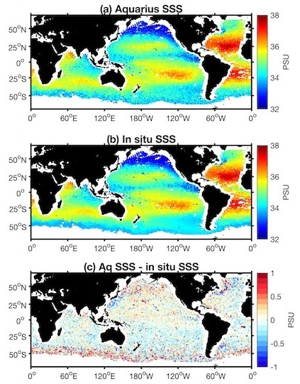
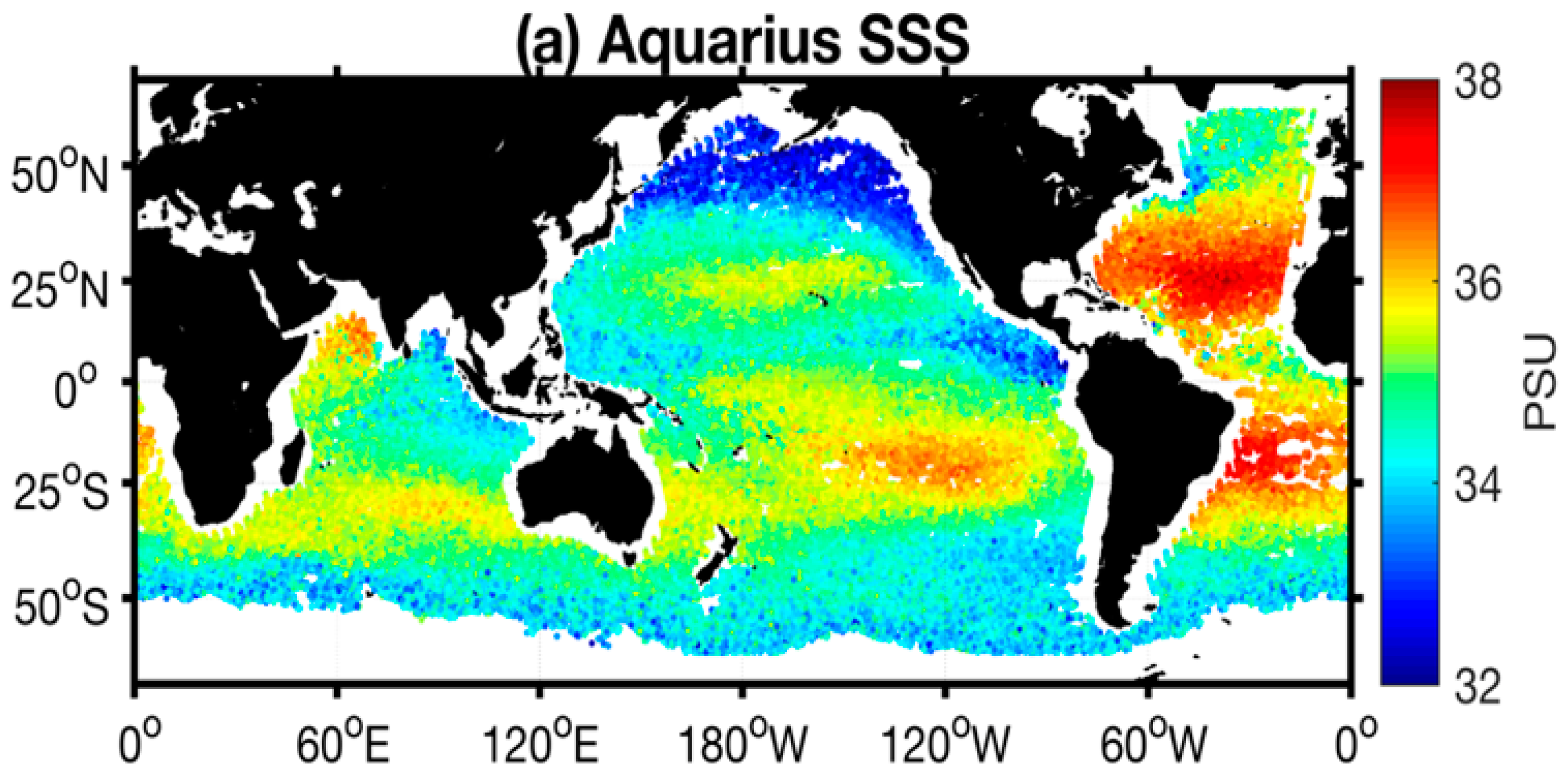
Figure 1a shows the Aquarius retrieved salinity at the in situ matchup points for all 45 months of observation from September 2011 to May 2015. The results are obtained from the AVDS. All the individual in situ salinity data at the same matchup points for the 45 months are shown in Figure 1b. The matchup processes are described in Section 2.3. The criterion for land fraction is set to 0.001, so the validation information is missing near the coasts due to the land contamination. The correspondence is visibly quite clear, with Aquarius Level-2 data resolving the salient large-scale ocean features. The SSS values in the open ocean generally range from 32 to 37 psu. Overall, Aquarius is able to accurately capture the SSS signature over the globe. High salinity is seen in the subtropical gyres, and the salinity maximum is located in the North Atlantic. Low salinity is observed in high latitudes, under the Intertropical Convergence Zone (ITCZ), and around major river outflows (including the Bay of Bengal). Figure 1c shows the Aquarius and in situ differences. Few anomalous values are observed near the islands. Positive biases up to 0.5 psu locally appear at high latitude (50 degrees poleward); they may be related to the galaxy reflection term that is not correctly adjusted for wind [16]. In the open ocean, only small differences (<0.2 psu) are generally present.
In the Northern Hemisphere, the negative biases in the eastern Atlantic and in the western Pacific are thought to be related to low-level radio frequency interference (RFI) from adjacent land that is not adequately detected by the standard RFI filter algorithm. This causes a positive brightness temperature bias and, thus, a negative salinity bias.
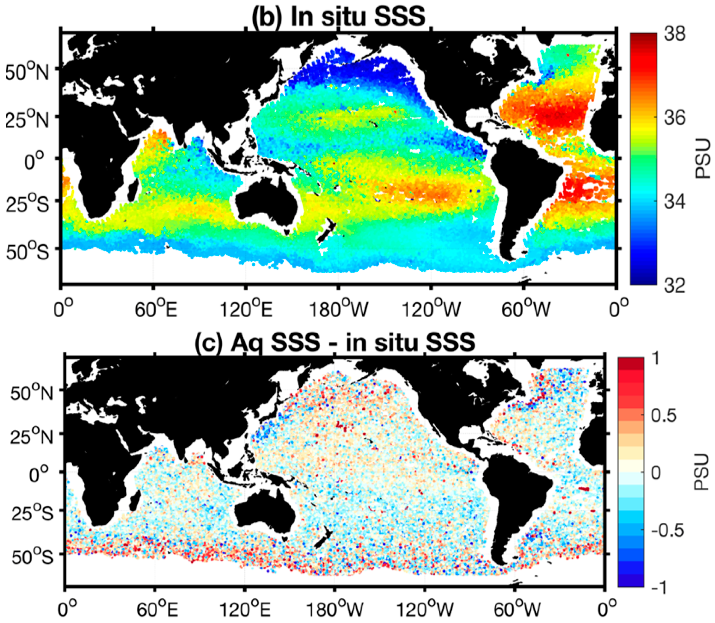
Figure 2 shows the time series of daily median of global differences between Aquarius SSS from each of the three beams and co-located in situ data from the AVDS analysis. The values of the standard deviation (STD), the square root of the variance, are also labeled in the figures. All three beams show small differences with little variations for the global median. The remaining differences may be related to the uncertainties of salinity observations, such as near-surface stratification or the sub-footprint variations [17]. The important conclusion from Figure 2 is that Aquarius measurements exhibit no spurious trends and drifts.
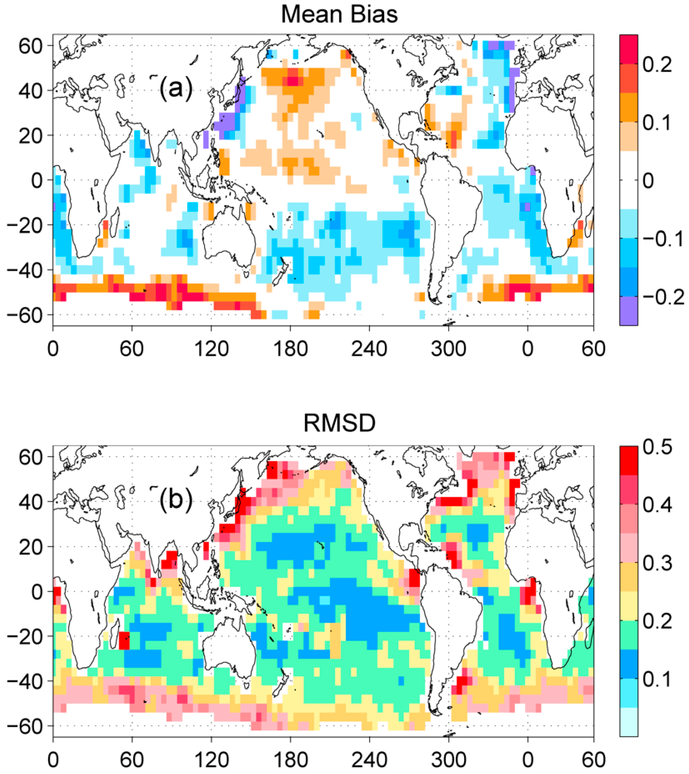
The time-mean bias error statistics for the Level-3 SSS rain-flagged product are presented in Figure 3. The error statistics were computed by comparing Argo float measurements from each profile for a given week with SSS values at the same locations obtained by interpolation of the corresponding Level-3 SSS maps. The root-mean-square deviation (RMSD) is defined as RMSD = sqrt(bias2 + STD2). The geographical distribution of the time-mean (static) Aquarius minus Argo differences is shown in Figure 3a. Large positive biases (up to 0.2 psu locally) are observed in the sub-polar North Pacific and in the Southern Ocean poleward of about 40°S. Large negative biases (up to −0.2 psu) are observed in the subtropical South Pacific and along the continental boundaries. These regions of positive and negative biases tend to cancel each other in the global average, producing nearly zero global bias (Figure 2). The regional biases shown in Figure 3a are similar to those shown in Figure 1c.
The RMSD between the weekly Level-3 analysis and concurrent Argo float data is smaller than 0.29 psu for nearly all weeks over the nearly 4-year period of comparison (not shown). The mean RMSD over the whole mission period (September 2011 through May 2015) is 0.247. The geographical distribution of the RMSD for the weekly Level-3 product is shown in Figure 3b. The RMSD is computed in 8°-longitude by 8°-latitude bins to ensure an adequate number of collocations (>100) in each bin. Over most of the ocean, the RMSD between weekly SSS maps and collocated in situ data do not exceed 0.2 psu. Figure 3b also demonstrates that the largest RMSD, exceeding 0.2 psu, are found in the regions of strong variability in SSS, such as along the North Pacific and North Atlantic ITCZ, the North Pacific sub-polar front, the Gulfstream, and near outflows of major rivers such as the Amazon in the tropical North Atlantic. In this regard, the observed relatively large RMSD between the Aquarius and Argo float data in some areas are not necessarily due to errors in Aquarius measurements only, but RMSD may include the disparity between time and space scales captured by two different observational platforms [17,18,19] and the difference in measurement depth between Aquarius (ocean surface) and Argo (~5 m depth) [17]. Larger bias and RMSD is also observed in the high latitudes. As mentioned in the introduction, this is partly due to lower measurement sensitivity of L-band brightness temperature to salinity in high-latitude oceans (relatively low SST).
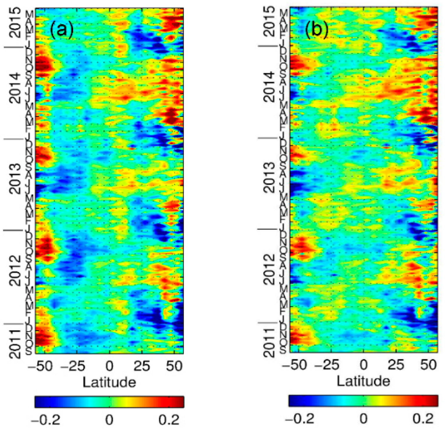
To examine temporal variability in the bias fields, Figure 4 shows the latitude-time distribution of the zonally averaged differences between the weekly Aquarius SSS maps and the corresponding Argo data. The zonally averaged biases are calculated weekly by averaging these statistics over 5°-latitude bins. The latitude-time distribution shows significant positive biases at high latitudes and negative biases in the subtropics. Besides the residual static bias, there is a clear seasonal cycle in the bias distribution. To emphasize the time-varying part, the 3-year average (September 2011 to August 2014) in each zonal bin is subtracted from the time series and is shown in Figure 4b. The peak-to-peak amplitude of the anomalous annual cycle can reach 0.2 psu locally. Whether this is significant or not depends on the amplitude of the “true” annual cycle in SSS and the signal-to-noise ratio.
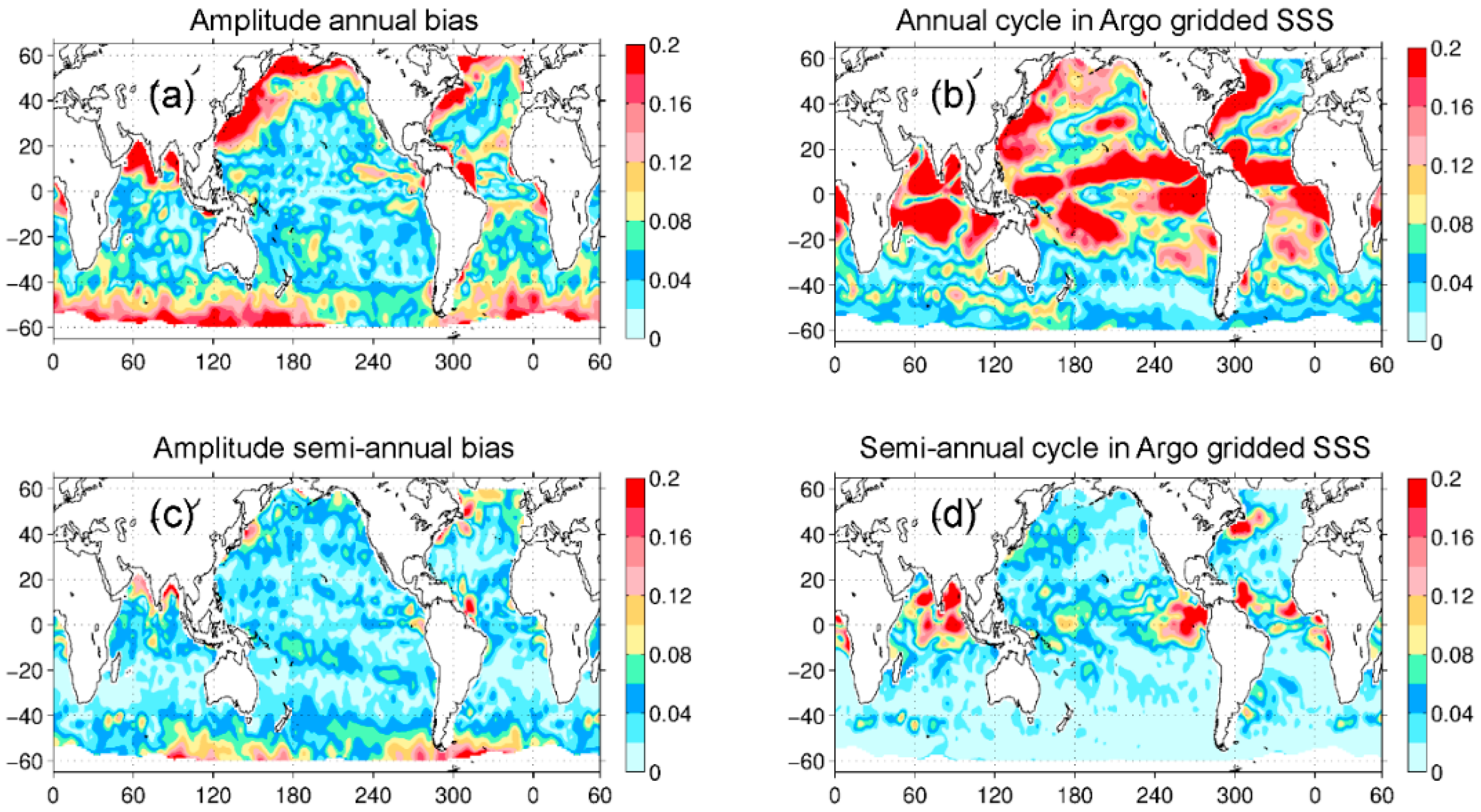
In Figure 5, the geographical distribution of the seasonal signal in Aquarius SSS is assessed against the seasonal cycle in the Argo-SIO gridded SSS. Because the Argo-derived product is very smooth, to match the spatial scales, the weekly Level-3 SSS maps from Aquarius were smoothed with a 2D running Hanning window of half-width of 4°, generally consistent with the smoothness properties of the Argo-derived salinity fields. The annual and semi-annual variations of the differences between Aquarius and Argo data are calculated from the harmonic analysis.
The amplitudes of the annual harmonic in the bias fields are presented in Figure 5a. Over most of the ocean, the amplitude of the annual signal in the Aquarius and Argo SSS differences is smaller than 0.05 psu. There are a few areas, however, where the amplitudes can reach 0.2 psu and more: The western boundary areas in the North Pacific and North Atlantic, the eastern boundary region of the North Atlantic, a zonal band going along the Southern Ocean, the Bay of Bengal and the Arabian Sea in the Indian Ocean, as well as a relatively small area in the eastern equatorial Pacific. Compared to the annual cycle in the Argo gridded SSS data (Figure 5b), the difference from the annual signal in Aquarius SSS appears to be minor, except for the areas where the vertical salinity gradient is known to be large. Although the relatively sparse sampling of Argo measurements in these regions may contribute to the differences in seasonal variability between Aquarius and Argo data, Aquarius data users are advised to exercise caution when analyzing seasonal variability in these areas considering the fundamental differences in how these observations are taken.
The amplitudes of the semi-annual harmonic in the bias fields are presented in Figure 5c. For comparison, the amplitudes of the semi-annual cycle in the Argo-derived SSS fields are presented in Figure 5d. Although generally small compared to the annual cycle biases, the semi-annual harmonic in the time-varying bias can be important compared to the Argo-derived variability regionally. Significantly affected areas are in the subtropical South Pacific, particularly along a quasi-zonal band stretching across the basin from about 30°S in the east to close to the equator in the west, and along the Southern Ocean.
It is worth emphasizing here that although an attempt has been made to quantify seasonal biases in Aquarius SSS, the results should rather be viewed as qualitative, serving as both a guidance and a note of caution, especially in light of potentially inadequate sampling of the Argo measurements in regions with strong intraseasonal variability.
3.2. Evaluation of Aquarius Level-3 SSS Data at Different Spatial Scales
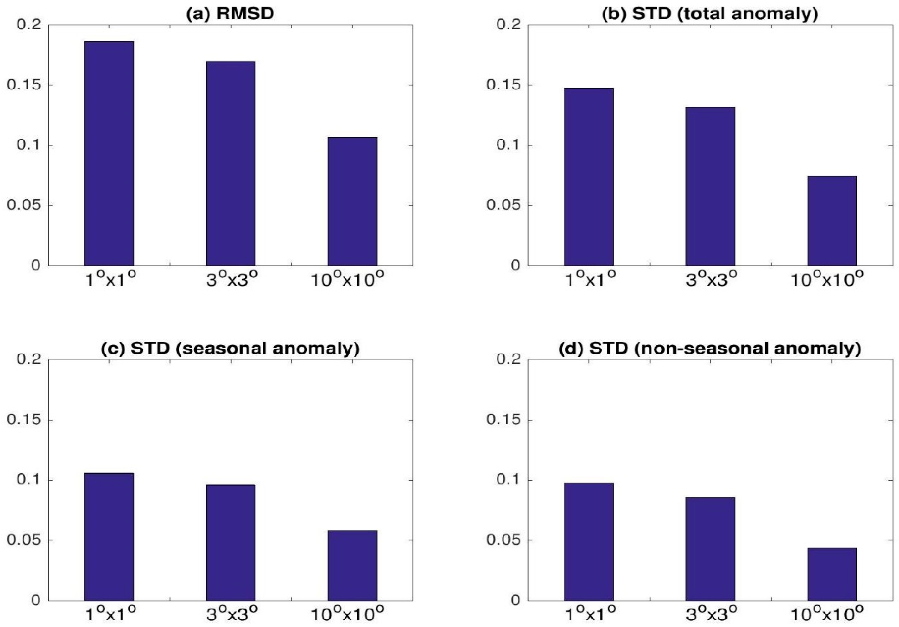
Figure 6a shows the global average value of the regional temporal RMSD between Aquarius and Argo-SIO SSS for 1° × 1°, 3° × 3°, and 10° × 10° scales. The RMSD decreases with larger smoothing scale. The RMSD are 0.19, 0.17, and 0.11 psu, respectively. The RMSD values include the contributions of differences in time-mean values and differences for temporal anomalies (deviation from time mean) between Aquarius and Argo SSS. Many applications do not concern time-mean biases but focus on variability (e.g., temporal and spatial changes). Therefore, we also assess the STD of the differences between Aquarius and Argo SSS. The time-mean differences between Aquarius and Argo products do not contribute to the STD values as they do to the RMSD values.
Figure 6b shows the global averages of regional temporal STD values of Aquarius SSS with respect to Argo-SIO SSS for various spatial scales. The difference between Figure 6a,b is that the latter excluded the time-mean biases of Aquarius SSS. The global average STD values for the 1° × 1°, 3° × 3°, and 10° × 10° scales are 0.15, 0.13, and 0.07 psu, respectively. Note that the RMSD and STD values with respect to Argo-SIO not only contain the errors of the Aquarius SSS, but the errors of the Argo-gridded product as well. Vinogradova and Ponte [18] Compared the Argo-SIO and Argo-APDRC gridded products and found a global average STD value of 0.10, 0.09, and 0.04 psu on the 1° × 1°, 3° × 3°, and 10° × 10° scales for the differences between the monthly Argo-SIO and Argo-APDRC products (Figure 1 in [20]). These values reflect the sampling error of individual Argo float data to represent the averages on different spatial scales as well as the mapping error of the Argo gridded products.
Figure 6c,d shows the global average of STD values for composite seasonal anomalies and non-seasonal anomalies (referenced to the composite seasonal cycle) of the SSS differences between Aquarius and Argo-SIO. The non-seasonal anomalies are associated with the differences between Aquarius and Argo-SIO in representing non-seasonal signals associated with phenomena such as tropical instability waves [4,21], Madden-Julian Oscillation [22,23], El Niño-Southern Oscillation [24], and Indian Ocean Dipole [25]. It is noteworthy that the global average STD value for non-seasonal SSS anomalies is less than 0.1 psu for 1° × 1° scale and 0.04 psu for 10° × 10° scale. Again, these values include the uncertainties of the Argo gridded product on these spatial and temporal scales.
The RMSD and STD values of Aquarius-Argo SSS differences are not only due to the uncertainty of Aquarius SSS, but also the uncertainty of the Argo gridded datasets as well. This is because Argo float distributions are too sparse to produce robust monthly mean values at 1° × 1° scale in regions with strong spatiotemporal variability such as tropical rain bands (e.g., under the ITCZ), near river plumes, western boundary currents, and the Antarctic Circumpolar Current. High-resolution in-situ thermosalinograph (TSG) data indeed show significant variations of SSS within the scales of Aquarius footprint [17]. Therefore, the Argo gridded data in these regions can be significantly affected by the sampling errors of the Argo array. In fact, Lee [20] found that the STD values between two of the Argo-SIO and Argo-APDRC products are as large as or even larger than the STD values between Aquarius and either of the Argo product in some of these regions.
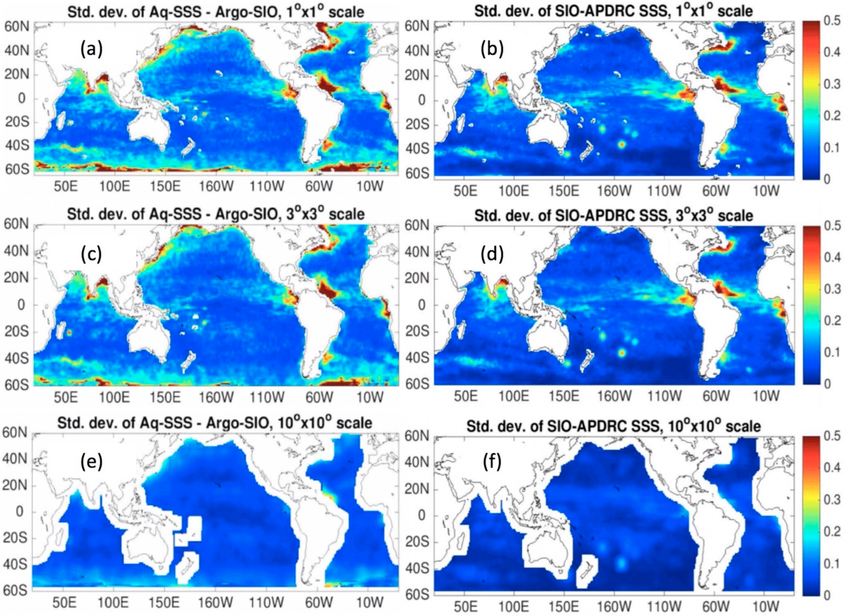
This is also reflected in Figure 7 by comparing the STD maps for Aquarius-Argo salinity for various resolutions of the Aquarius data as well as the STD for the difference between Argo-SIO and Argo-APDRC data. This issue also exists for the comparison of STD on 3° × 3° scale (Figure 7c,d). However, for the 10° × 10° scale, Argo data have sufficient sampling to represent the large scale monthly mean values, so the difference between the two Argo products is much smaller (Figure 7e,f). The message for the comparison shown in Figure 7 is that RMSD and STD values of the difference between Aquarius and Argo gridded data can be used as an indication of Aquarius data uncertainty. However, these values also contain the sampling uncertainty associated with the data products generated from the individual Argo profiles.
3.3. Triple-Point Analysis of Aquarius, In Situ, and HYCOM
As discussed earlier, the differences between Aquarius and in-situ measurements contain uncertainties of the Aquarius data, as well as the effect of sampling differences between Aquarius and in situ measurements. It is therefore of interest to estimate the uncertainty of the in situ data in representing the truth on the spatiotemporal scales of the Aquarius measurements, as well as the uncertainty of the Aquarius measurements that take into account the representativeness error of the in-situ measurements on Aquarius’ measurement scales. One such approach is the so-called triple collocation analysis or triple-point analysis (Appendix A). Here, we apply the triple-point approach to assess the Aquarius root mean square error (RMSE) by taking into consideration the representativeness error of the in situ measurements on Aquarius measurement scales. From the bias and standard deviation (STD) differences between the Aquarius data and in situ observations, the root mean square deviation (RMSD) is obtained as the square-root of the (bias2 + STD2). The RMSD per se includes both the Aquarius SSS error and the effect due to the sampling differences between Aquarius and in situ measurement, whereas our goal here is to isolate the Aquarius RMSE. The detailed formulas used to calculate the RMSE are documented in Appendix A.
The triple-point analysis requires three independent datasets. Here we use the HYCOM operational ocean analysis (a data-assimilation product), in addition to the Aquarius SSS and in-situ measurements. See Appendix A in the Aquarius user guide for more details about HYCOM data. Aquarius data are independent of HYCOM as the Aquarius satellite information is not used for HYCOM assimilation. Note that HYCOM assimilates Argo measurements, which account for the majority of in-situ measurements over the global ocean as a whole. In this sense, HYCOM is not fully independent from in situ measurements. However, HYCOM salinity is not only constrained by Argo measurements, but also by evaporation-precipitation forcing, ocean dynamics, and a relaxation of model SSS to a seasonal climatology to prevent model drift. These factors help maintain some level of independence of HYCOM SSS from in-situ measurements. Nevertheless, the results of the triple-point analysis is to some extent affected by the assumption that the three datasets are independent.
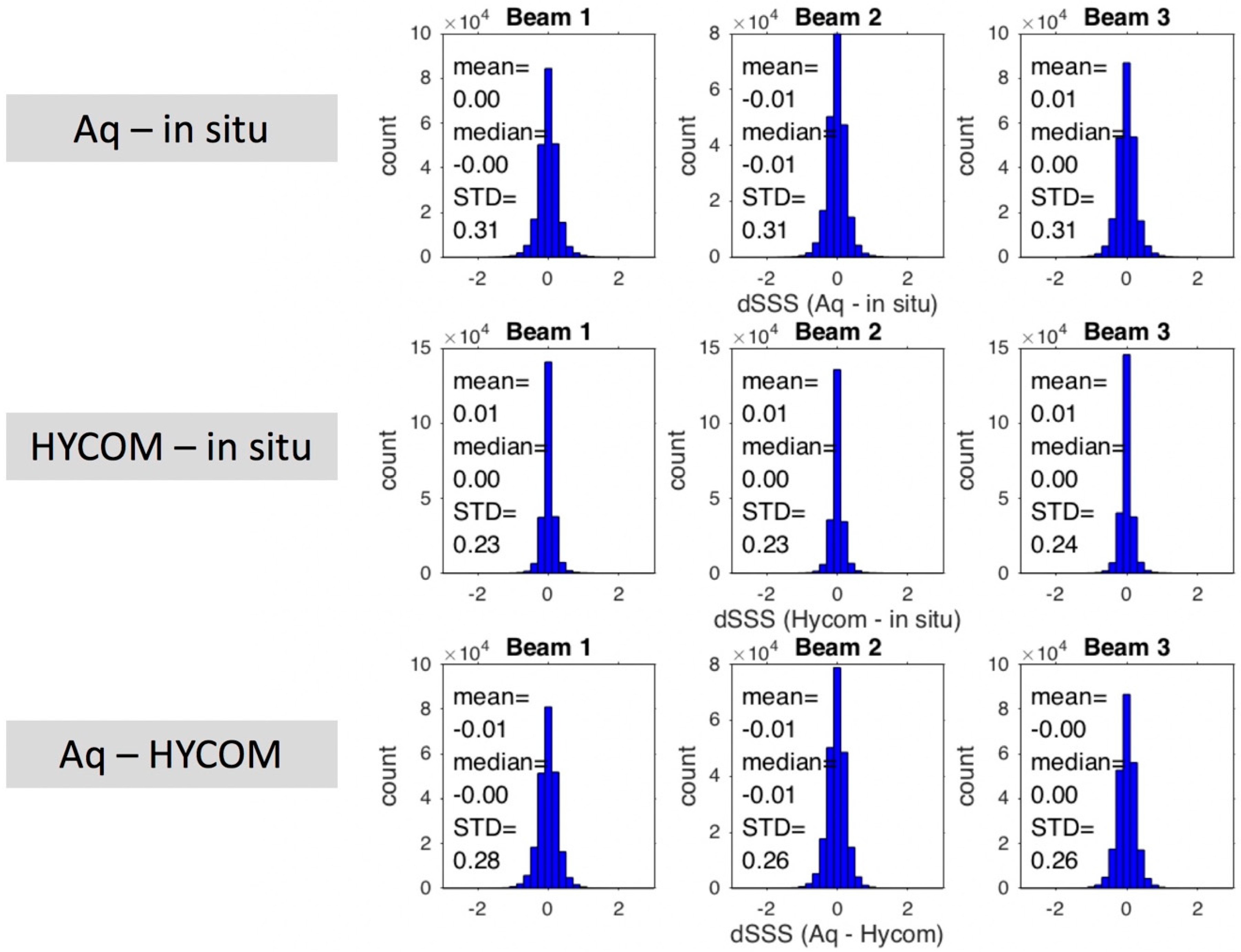
Figure 8 gives the matchup statistics for Aquarius-in situ, HYCOM-in situ, and Aquarius-HYCOM (at the in situ locations), for each of the three beams. Note that all three data sets are biased ≤|0.01| relative to each other, on average, at all Aquarius beam locations. The root-mean-square deviation (RMSD) is defined as RMSD = sqrt(bias2 + STD2). Figure 8 shows HYCOM-in situ RMSD ~0.23 psu overall. The RMSD for Aquarius-in situ and Aquarius-HYCOM are 0.31 psu and 0.27 psu, respectively. The co-located statistics allow us to estimate the root-mean-square error (RMSE) of each of the three measurements. The results of Aquarius co-located matchup points are given in Table 1. The Aquarius, HYCOM and in situ RMSE are approximately 0.17 psu, 0.08 psu, and 0.14 psu, respectively. Recall that these Aquarius matchup statistics are for individual match-ups, with no averaging.
For the Level-3 SSS error analysis, the three data sets for the triple-point collocation are (1) Aquarius ADPS Level-3 data; (2) similarly gridded HYCOM SSS monthly 1° × 1° maps; and (3) the in situ data set (un-gridded). Next, we find the RMSD of three data pairs: (1) Aquarius-in situ; (2) HYCOM-in situ; and (3) Aquarius-HYCOM. The process finds all the in situ data points within the mapped 1° × 1° boxes for each month, averages those, differences that from the gridded monthly value for that grid-box, and then computes the RMSD of all the matched 1° × 1° grid-boxes over the globe for that month. Aquarius-HYCOM is simply the RMSD between the respective monthly 1° × 1° maps. The RMSD accumulations also ensure that only the 1° × 1° grid boxes containing in situ samples are counted, to ensure common sampling. We also note that the standard Level-3 gridding masks and flags are applied; thus, cold regions (SST < 5°C) and regions higher than the threshold for land contamination are omitted (See Table 1 in AQ-014-PS-0018_AquariusLevel2specification_DatasetVersion5.0 for the description of data quality flags and masks).
The triple-point analyses giving estimated RMSE of each measurement system (Aquarius, HYCOM, in situ) are presented in Table 2. Note that the largest RMSE belongs to the in situ data. These are a combination of in situ measurement and representativeness errors. The latter include spatial and temporal variations of the in situ observations within the 1 × 1 grid box during the month, plus the salinity differences between the in situ sampling depths and the surface. However, the results from such an analysis are sometimes met by skepticism because of the assumptions such as independent errors among the three products and usage of model-based ground truth (HYCOM).
The Aquarius monthly RMSE estimates are <0.2 psu for all months of the mission, and the average over all months is 0.128 psu. Given that 0.20 psu is the mission accuracy requirement for monthly average maps, this calculation verifies that the Aquarius data exceed the mission requirement 0.2 psu by a substantial margin.
3.4. Contrasting Ascending and Descending Passes
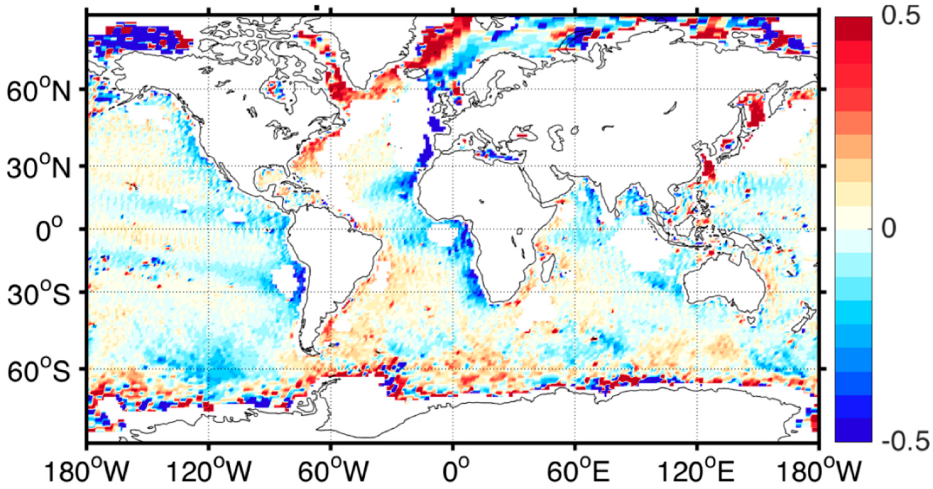
We now examine the differences of SSS between the ascending (northward, 6p.m.) and descending (southward, 6a.m.) orbits; the mission long average is shown in Figure 9. In principle, the ascending and descending maps are expected to be nearly identical. However, a large blue patch in the eastern Atlantic, and red zones in the western Atlantic and Asia-Pacific are observed. These ascending and descending differences are related to the RFI. The RFI asymmetry between ascending and descending tracks is the results of the opposite viewing angle (toward or away from the land emitting sources) between the two sides of the orbit. The antenna faces eastward on ascending passes and westward on descending passes.
In Figure 9, the RFI influenced areas, including both sides of the Atlantic Ocean, eastern Indian Ocean, and the northwestern Pacific are masked out for the large ascending minus descending differences. Users should note that regions with excessive ascending and descending differences due to RFI are masked when mapping. This shows gaps in the maps of only ascending or only descending passes. The ascending masked regions differ from the descending ones, and do not overlap. See AQ-014-PS-0006_ProposalForFlags&Masks_DatasetVersion3.0, which is included in the Data Version V5.0 documentation. There are visible ascending and descending differences at high southern latitudes. One can see a zonal variation between light blue and light red blobs around 60°S. It is not clear at this point what the reasons are for these ascending minus descending differences.
4. Discussion and Conclusions
In this paper, the quality of Aquarius SSS data has been evaluated with multiple approaches. Regarding the data accuracy on monthly 1° × 1° scales, the results consistently demonstrate that the estimated errors are less than the mission requirement of 0.2 psu. The triple-point analysis resolved RMSE ~0.17 psu for point comparisons (no monthly averaging). On monthly time scales, triple-point analysis demonstrated a nominal RMSE ~0.128 psu, improving on the mission requirement by a substantial margin. Figure 3 shows that over most of the ocean, the RMSD between weekly SSS maps and collocated in situ data do not exceed 0.2 psu. Figure 6 demonstrates that the monthly, global average RMSD between gridded Aquarius and Argo data is smaller than 0.2 psu. All of these results present consistent evidence that the Aquarius Ocean Salinity Mission has met the measurement accuracy requirement.
However, the following notes of caution need to be provided to data users.
Localized persistent biases between ascending and descending passes exist in the areas close to the continental boundaries. They could be linked to radio frequency interference (RFI) that is not completely corrected by the RFI filter. The RFI will bias the brightness temperatures toward the positive, thus the salinity will be biased negative. These regions are primarily in the eastern North Atlantic adjacent to Europe where it is likely that the ascending pass is contaminated as the antenna faces the European subcontinent. Likewise, the western North Atlantic and Asia-Pacific regions are biased on the descending pass when the antenna views westward. The radiometer flag is added in the data files to exclude the area with unacceptable ascending and descending differences. This flag identifies areas where the ascending and descending difference is sufficiently large that the data from the out-of-bound pass (i.e., either ascending or descending) is discarded for purposes of calibration. Users should be very cautious with using ascending pass data in the eastern North Atlantic and descending pass data in the western North Atlantic and Asia-Pacific regions.
It is strongly recommended that data users use caution when analyzing or drawing conclusions about the annual salinity cycle in the Aquarius data, because the variability may be contaminated by spurious, non-oceanographic, error signals, especially in the Southern Hemisphere and higher latitudes, as shown in Figure 4 and Figure 7. At high-latitude oceans, the L-band radiometer has poor sensitivity to SSS related to the low SST. This is a fundamental issue for L-band radiometry that needs technology innovation to solve [2,16]. Although most of the validation results shown in this paper are based on the Level-3 product, similar caution should be used when analyzing the along-track, Level-2 data, including RFI-affected regions, latitudinal biases, ascending and descending biases.
The rain filters (instantaneous rain rates >0.25 mm/h) are applied for the Aquarius calibration, so the strong precipitation events, which introduce large vertical stratification and large SSS biases, do not dominate the SSS variations on global average. If the users are interested in the Aquarius SSS under strong precipitation, the data without rain masks should be used. Otherwise, data with rain masks should be used for general studies. The users can tell if the data have been rain masked from the file titles.
Author Contributions
T.M. designed the basics of salinity retrieval algorithms for Aquarius, and implemented the changes that were developed for Aquarius Version 5. G.S.E.L. designed the AVDS and developed the triple-point analysis; H.-Y.K., T.L. and O.M. performed the Aquarius salinity validation; H.K. wrote the paper; P.H. provided input for the validation analysis and edition of the manuscripts.
Funding
This study was supported by NASA Ocean Salinity Science Team through grants NNX17AK16G, NNX17AK06G, and grant NNX14AJ02G. This paper is IPRC/SOEST contribution 10436/1338.
Acknowledgments
We thank David LeVine (NASA Goddard Space Flight Center), Liang Hong (Science Application Intl. Corp.), and Jorge Vazquez (Jet Propulsion Lab) for useful comments for the Aquarius validation document. We also thank the Aquarius cal/val team for the improvement of the Aquarius data.
Conflicts of Interest
The authors declare no conflicts of interest.
Appendix A
The satellite salinity measurement SS and the in situ validation measurement SV are defined by:
where S is the true surface salinity averaged over the Aquarius footprint area and microwave optical depth in seawater (~1 cm). εS and εV are the respective satellite and in situ measurement errors relative to S. The mean square of the difference ΔS between SS and SV is given by:
where < > denotes the average over a given set of paired satellite and in situ measurements, and <εS εV > = 0. Likewise, define HYCOM salinity interpolated to the satellite footprint as SH = S ± εH, and mean square differences
SS = S ± εS,
SV = S ± εV,
<ΔSSV2> = <εS2> + <εV2>,
HYCOM vs. in situ validation data
satellite vs. HYCOM
<ΔSHV2> = <εH2> + <εV2>
<ΔSSH2> = <εS2> + <εH2>
Equations (1)–(3) comprise three equations with three variables given by:
Satellite measurement
<εS2> = {<ΔSSV2> + <ΔSSH2>−<ΔSHV2>}/2
HYCOM measurement
<εH2> = {<ΔSSH2> + <ΔSHV2>−<ΔSSV2>}/2
In situ validation measurement
<εV2> = {<ΔSSV2> + <ΔSHV2>−<ΔSSH2>}/2
References
- Lagerloef, G.; Colomb, R.; Le Vine, D.; Wentz, F.; Yueh, S.; Ruf, C.; Lilly, J.; Gunn, J.; Chao, Y.; de Charon, A.; et al. The Aquarius/SAC-D mission—Designed to Meet the Salinity Remote Sensing Challenge. Oceanography 2008, 21, 68–81. [Google Scholar] [CrossRef]
- Le Vine, D.M.; Dinnat, E.P.; Meissner, T.; Wentz, F.J.; Kao, H.-Y.; Lagerloef, G.; Lee, T. Status of Aquarius and salinity continuity. Remote Sens. 2018. submitted. [Google Scholar]
- Kao, H.-Y.; Lagerloef, G.S.E. Salinity fronts in the tropical Pacific Ocean. J. Geophys. Res. Oceans 2015, 120, 1096–1106. [Google Scholar] [CrossRef] [PubMed] [Green Version]
- Lee, T.; Lagerloef, G.; Gierach, M.M.; Kao, H.-Y.; Yueh, S.; Dohan, K. Aquarius reveals salinity structure of tropical instability waves. Geophys. Res. Lett. 2012, 39, L12610. [Google Scholar] [CrossRef]
- Grodsky, S.A.; Reul, N.; Lagerloef, G.; Reverdin, G.; Carton, J.A.; Chapron, B.; Quilfen, Y.; Kudryavtsev, V.N.; Kao, H.-Y. Haline hurricane wake in the Amazon/Orinoco plume: AQUARIUS/SACD and SMOS observations. Geophys. Res. Lett. 2012, 39, L20603. [Google Scholar] [CrossRef]
- Melnichenko, O.V.; Amores, A.; Maximenko, N.A.; Hacker, P.; Potemra, J.T. Signature of mesoscale eddies in satellite sea surface salinity data. J. Geophys. Res. Oceans 2017, 122, 1416–1424. [Google Scholar] [CrossRef]
- Kao, H.-Y.; Lagerloef, G.; Lee, T.; Melnichenko, O.; Hacker, P. Aquarius Salinity Validation Analysis; Data Version 5.0. 2017. Available online: Ftp://podaac-ftp.jpl.nasa.gov/allData/aquarius/docs/v5/AQ-014-PS-0016_AquariusSalinityDataValidationAnalysis_DatasetVersion5.0.pdf (accessed on 21 August 2018).
- Meissner, T. Assessment of Uncertainties in Aquarius Salinity Retrievals. 2015. Available online: Ftp://podaac-ftp.jpl.nasa.gov/allData/aquarius/docs/v4/AQ-014-PS-0017_AquariusATBD_uncertainties_Addendum5_DatasetVersion4.0.pdf (accessed on 21 August 2018).
- Le Vine, D.M.; Lagerloef, G.S.E.; Colomb, F.R.; Yueh, S.H.; Pellerano, F.A. Aquarius: An instrument to monitor sea surface salinity from Space. IEEE Trans. Geosci. Remote Sens. 2007, 45, 2040–2050. [Google Scholar] [CrossRef]
- Piepmeier, J. Aquarius Radiometer Post-Launch Calibration for Product Version 2. 2013. Available online: Ftp://podaac-ftp.jpl.nasa.gov/allData/aquarius/docs/v2/AQ-014-PS-0015_AquariusInstrumentCalibratrionDescriptionDocument.pdf (accessed on 21 August 2018).
- Lagerloef, G.; Kao, H.-Y.; Hacker, P.; Hackert, E.; Chao, Y.; Hilburn, K.; Meissner, T.; Yueh, S.; Liang, H.; Lee, T. 2013: Aquarius Salinity Validation Analysis; Data Version 2.0. Available online: https://aquarius.umaine.edu/docs/AQ-014-PS-0016_AquariusSalinityDataValidationAnalysis_DatasetVersion2.0.pdf (accessed on 21 August 2018).
- Brasnett, B. The impact of satellite retrievals in a global sea-surface-temperature analysis. Q. J. R. Meteorol. Soc. 2008, 134, 1745–1760. [Google Scholar] [CrossRef] [Green Version]
- Meissner, T.; Wentz, F.; Le Vine, D. Aquarius Salinity Retrieval Algorithm: Algorithm Theoretical Basis Document (ATBD) End of Mission Version. 2017. Available online: Ftp://podaac-ftp.jpl.nasa.gov/allData/aquarius/docs/v5/AQ-014-PS-0017_Aquarius_ATBD-EndOfMission.pdf (accessed on 21 August 2018).
- Chassignet, E.P.; Hurlburt, H.E.; Metzger, E.J.; Smedstad, O.M.; Cummings, J.; Halliwell, G.R.; Bleck, R.; Baraille, R.; Wallcraft, A.J.; Lozano, C.; et al. GODAE: Global Ocean Prediction with the HYbrid Coordinate Ocean Model (HYCOM). Oceanography 2009, 22, 64–75. [Google Scholar] [CrossRef]
- Lilly, J.; Lagerloef, G. Aquarius Level 3 Processing Algorithms Theoretical Basis Document. 2008. Available online: Ftp://podaac-ftp.jpl.nasa.gov/allData/aquarius/docs/v2/AquariusLevel3_GriddingSmoothingPaper_Lilly&Lagerloef2008.pdf (accessed on 21 August 2018).
- Meissner, T.; Wentz, F.J.; Le Vine, D. The salinity retrieval algorithm for the NASA Aquarius Version 5 and SMAP Version 3 Releases. Remote Sens. 2018, 10, 1121. [Google Scholar] [CrossRef]
- Boutin, J.; Chao, Y.; Asher, W.E.; Delcroix, T.; Drucker, R.; Drushka, K.; Kolodziejczyk, N.; Lee, T.; Reul, N.; Reverdin, G.; et al. Satellite and in situ salinity: Understanding near surface stratification and sub-footprint variability. Bull. Am. Meteorol. Soc. 2016, 97, 1391–1407. [Google Scholar] [CrossRef]
- Vinogradova, N.T.; Ponte, R.M. Assessing temporal aliasing in satellite-based surface salinity measurements. J. Atmos. Ocean. Technol. 2012, 29, 1391–1400. [Google Scholar] [CrossRef]
- Vinogradova, N.T.; Ponte, R.M. Small-scale variability in sea surface salinity and implications for satellite-derived measurements. J. Atmos. Ocean. Technol. 2013, 30, 2689–2694. [Google Scholar] [CrossRef]
- Lee, T. Consistency of Aquarius sea surface salinity with Argo products on various spatial and temporal scales. Geophys. Res. Lett. 2016, 43, 3857–3864. [Google Scholar] [CrossRef]
- Lee, T.G.; Lagerloef, H.-Y.; Kao, M.; Willis, J.; Gierach, M. The influence of salinity on tropical Atlantic instability waves. J. Geophys. Res. Oceans 2014, 119, 8375–8394. [Google Scholar] [CrossRef] [Green Version]
- Grunseich, G.; Subrahmanyam, B.; Wang, B. The Madden-Julian oscillation detected in Aquarius salinity observations. Geophys. Res. Lett. 2013, 40, 5461–5466. [Google Scholar] [CrossRef] [Green Version]
- Guan, B.; Lee, T.; Halkides, D.; Waliser, D.E. Aquarius surface salinity and the Madden-Julian Oscillation: The role of salinity in surface layer density and potential energy. Geophys. Res. Lett. 2014, 41, 2858–2869. [Google Scholar] [CrossRef] [Green Version]
- Qu, T.D.; Yu, J.Y. ENSO indices from sea surface salinity observed by Aquarius and Argo. J. Oceanogr. 2014, 70, 367–375. [Google Scholar] [CrossRef] [Green Version]
- Du, Y.; Zhang, Y. Satellite and Argo observed surface salinity variations in the Tropical Indian Ocean and their association with the Indian Ocean Dipole mode. J. Clim. 2015, 28, 695–713. [Google Scholar] [CrossRef]
Figure 1.
(a) Aquarius Level-2 and (b) in situ co-located salinity data gathered from September 2011 to May 2015. (c) The sea surface salinity (SSS) differences defined as the Aquarius minus the co-located in situ salinity.
Figure 1.
(a) Aquarius Level-2 and (b) in situ co-located salinity data gathered from September 2011 to May 2015. (c) The sea surface salinity (SSS) differences defined as the Aquarius minus the co-located in situ salinity.


Figure 2.
Time series of daily median of global Aquarius—in situ SSS in three beams. 7-day average is applied to smooth the data. The median and the standard deviation (STD) labeled in the figures are based on the average of differences for the whole mission period from September 2011 to May 2015.
Figure 2.
Time series of daily median of global Aquarius—in situ SSS in three beams. 7-day average is applied to smooth the data. The median and the standard deviation (STD) labeled in the figures are based on the average of differences for the whole mission period from September 2011 to May 2015.

Figure 3.
Geographical distribution of (a) mean spatial bias (psu), and (b) root-mean-square deviation (RMSD) (psu) between the Aquarius weekly Level-3 SSS product and Argo float observations. The error statistics were computed by comparing Argo float measurements for a given week with SSS values at the same locations obtained by interpolation of the corresponding Level-3 SSS maps. The geographical distributions are computed in 8°-longitude by 8°-latitude bins.

Figure 4.
(a) Latitude-time distribution of the zonally averaged differences (psu) between the weekly Level-3 SSS maps and the corresponding Argo data. The error statistics were computed by comparing Argo float measurements for a given week with SSS values at the same locations obtained by interpolation of the corresponding Level-3 SSS maps. The zonally averaged biases were computed by averaging these statistics over 5°-latitude bins. (b) The same as in (a), but with the 3-year mean (September 2011 to August 2014) subtracted.

Figure 5.
(a) Amplitude of the annual cycle in the Aquarius minus Argo bias; (b) Amplitude of the annual cycle in SSS from the Argo-derived gridded SSS fields produced by the Scripps Institution of Oceanography (SIO); (c) Amplitude of the semi-annual cycle in the Aquarius minus Argo bias; (d) Amplitude of the semi-annual cycle in SSS from the Argo-derived gridded SSS fields produced by the SIO.

Figure 6.
(a) Global average of regional temporal RMSD values between Aquarius and Argo-SIO SSS on various spatial scales as indicated by legends along the horizontal axis. Global average of regional temporal STD values for the differences between Aquarius and Argo-SIO SSS on various spatial scales for (b) total anomalies; (c) composite seasonal anomalies; and (d) non-seasonal anomalies. All RMSD and STD values are in the unit of psu.

Figure 7.
The STD of the difference between Aquarius and Argo-SIO SSS on (a) 1° × 1°, (c) 3° × 3° and (e) 10° × 10° scale. The STD of the difference between Argo-SIO and Argo-APDRC are shown in (b), (d), and (f).
Figure 7.
The STD of the difference between Aquarius and Argo-SIO SSS on (a) 1° × 1°, (c) 3° × 3° and (e) 10° × 10° scale. The STD of the difference between Argo-SIO and Argo-APDRC are shown in (b), (d), and (f).

Figure 8.
Co-located difference histograms for each beam of Aquarius L2 data. (top) Aquarius—in situ, (middle) Hybrid Coordinate Ocean Model (HYCOM)—in situ, (bottom) Aquarius—HYCOM.
Figure 8.
Co-located difference histograms for each beam of Aquarius L2 data. (top) Aquarius—in situ, (middle) Hybrid Coordinate Ocean Model (HYCOM)—in situ, (bottom) Aquarius—HYCOM.

Figure 9.
Forty-five-month average of ascending–descending data. Major bias regions are described in the text. The “white” regions in the North Atlantic, Western Pacific (China, Japan) or Indonesia are masked out due to suspected undetected radio frequency interference (RFI). See flagging/masking tables in [9] for details.


Table 1.
Estimated Root Mean Square Error (RMSE) in the unit of psu for each data type based on the triple point analysis of co-located point measurements.
Table 1.
Estimated Root Mean Square Error (RMSE) in the unit of psu for each data type based on the triple point analysis of co-located point measurements.
| V5.0 | Beam 1 | Beam 2 | Beam 3 |
|---|---|---|---|
| Aquarius RMSE | 0.17 | 0.17 | 0.16 |
| HYCOM RMSE | 0.09 | 0.08 | 0.09 |
| In situ RMSE | 0.13 | 0.14 | 0.15 |
Table 2.
Triple-point analysis: Monthly Root Mean Square Error (RMSE) differences for Aquarius, Hybrid Coordinate Ocean Model (HYCOM), and in situ fields. Each panel represents one year (September–August) beginning September 2011. At the bottom of the fourth panel, green highlight, are the average RMSE over the 45 months. Note that the Aquarius mean value is 0.128 psu.

© 2018 by the authors. Licensee MDPI, Basel, Switzerland. This article is an open access article distributed under the terms and conditions of the Creative Commons Attribution (CC BY) license (http://creativecommons.org/licenses/by/4.0/).
Share and Cite
MDPI and ACS Style
Kao, H.-Y.; Lagerloef, G.S.E.; Lee, T.; Melnichenko, O.; Meissner, T.; Hacker, P. Assessment of Aquarius Sea Surface Salinity. Remote Sens. 2018, 10, 1341. https://0-doi-org.brum.beds.ac.uk/10.3390/rs10091341
AMA Style
Kao H-Y, Lagerloef GSE, Lee T, Melnichenko O, Meissner T, Hacker P. Assessment of Aquarius Sea Surface Salinity. Remote Sensing. 2018; 10(9):1341. https://0-doi-org.brum.beds.ac.uk/10.3390/rs10091341
Chicago/Turabian StyleKao, Hsun-Ying, Gary S. E. Lagerloef, Tong Lee, Oleg Melnichenko, Thomas Meissner, and Peter Hacker. 2018. "Assessment of Aquarius Sea Surface Salinity" Remote Sensing 10, no. 9: 1341. https://0-doi-org.brum.beds.ac.uk/10.3390/rs10091341
Note that from the first issue of 2016, this journal uses article numbers instead of page numbers. See further details here.