Visualizing the Spatiotemporal Trends of Thermal Characteristics in a Peatland Plantation Forest in Indonesia: Pilot Test Using Unmanned Aerial Systems (UASs)


Abstract
:
1. Introduction
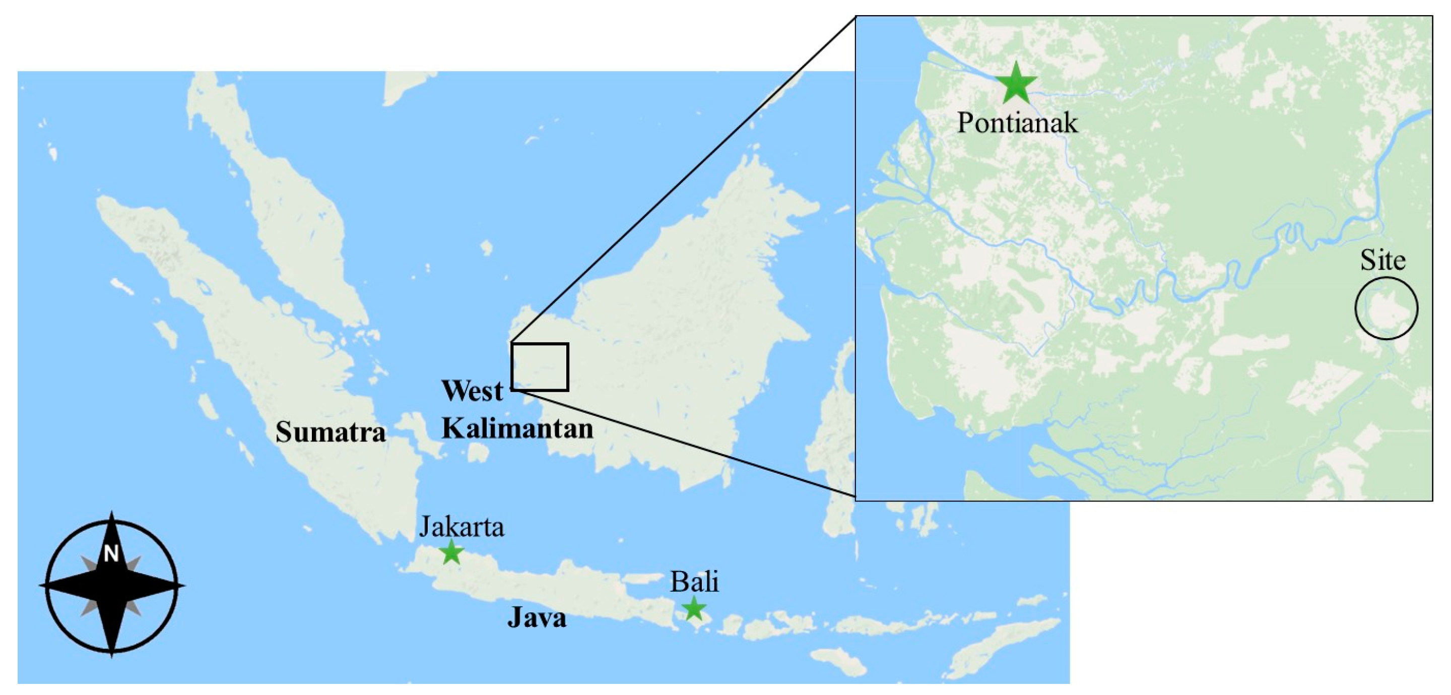
2. Study Area
3. Materials and Methods
3.1. UAS and Thermal Camera Image Processing
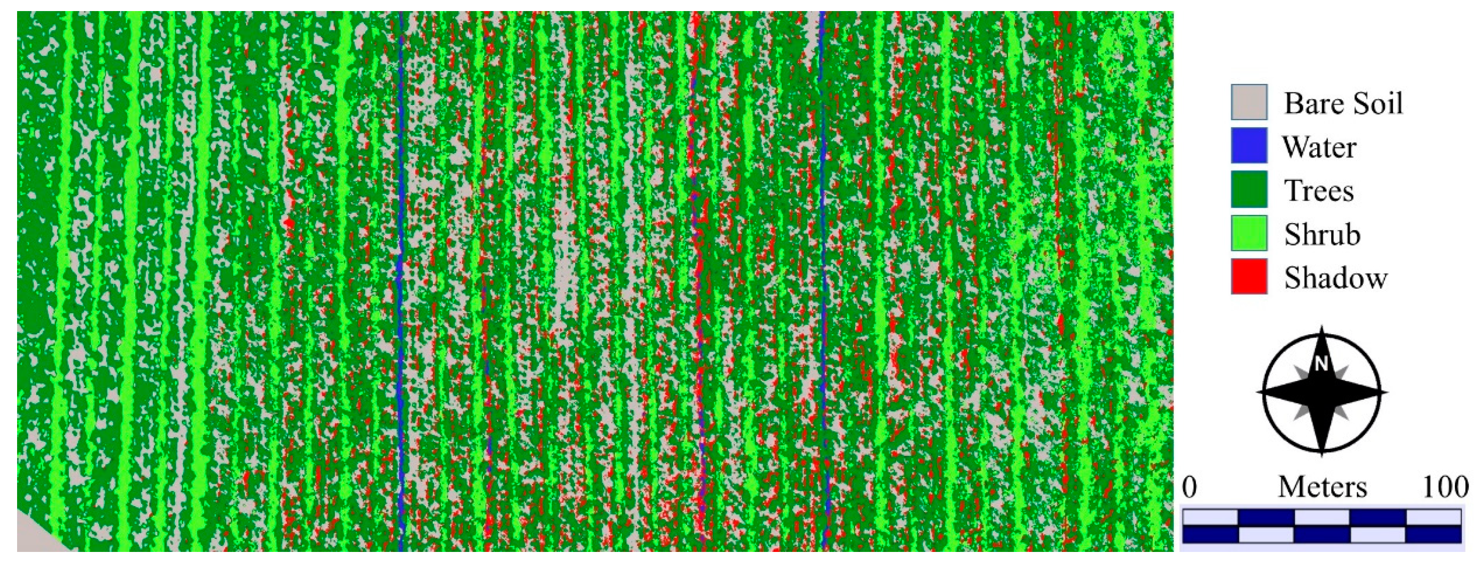
3.2. Image Classification
3.3. Principal Component Analysis (PCA) of Thermal Images
4. Results
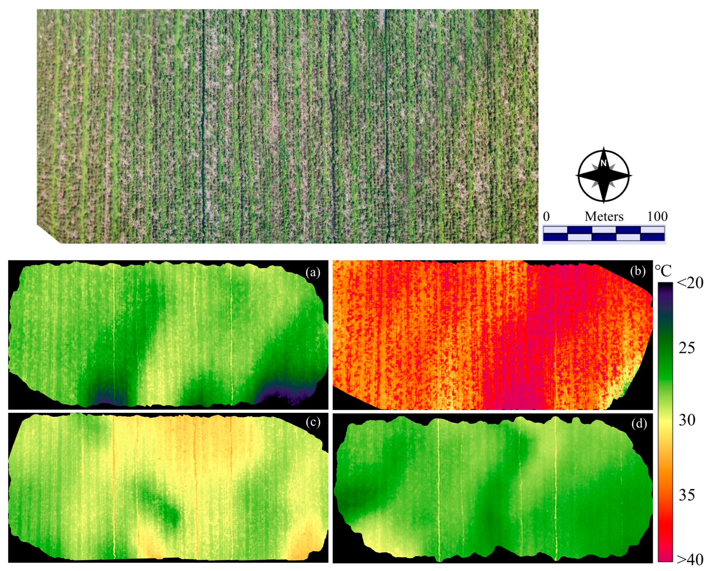
4.1. Mapping of the RGB, Thermal, and Classification Maps
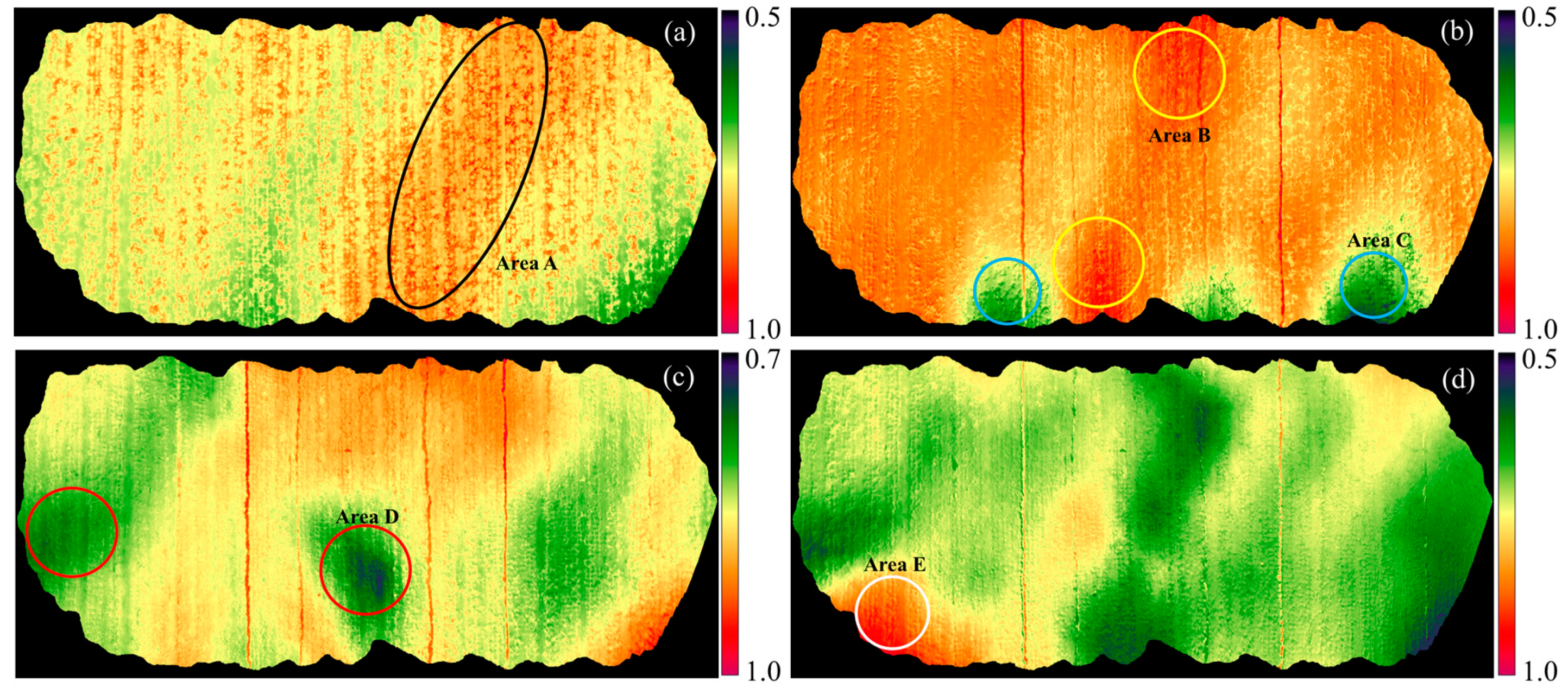
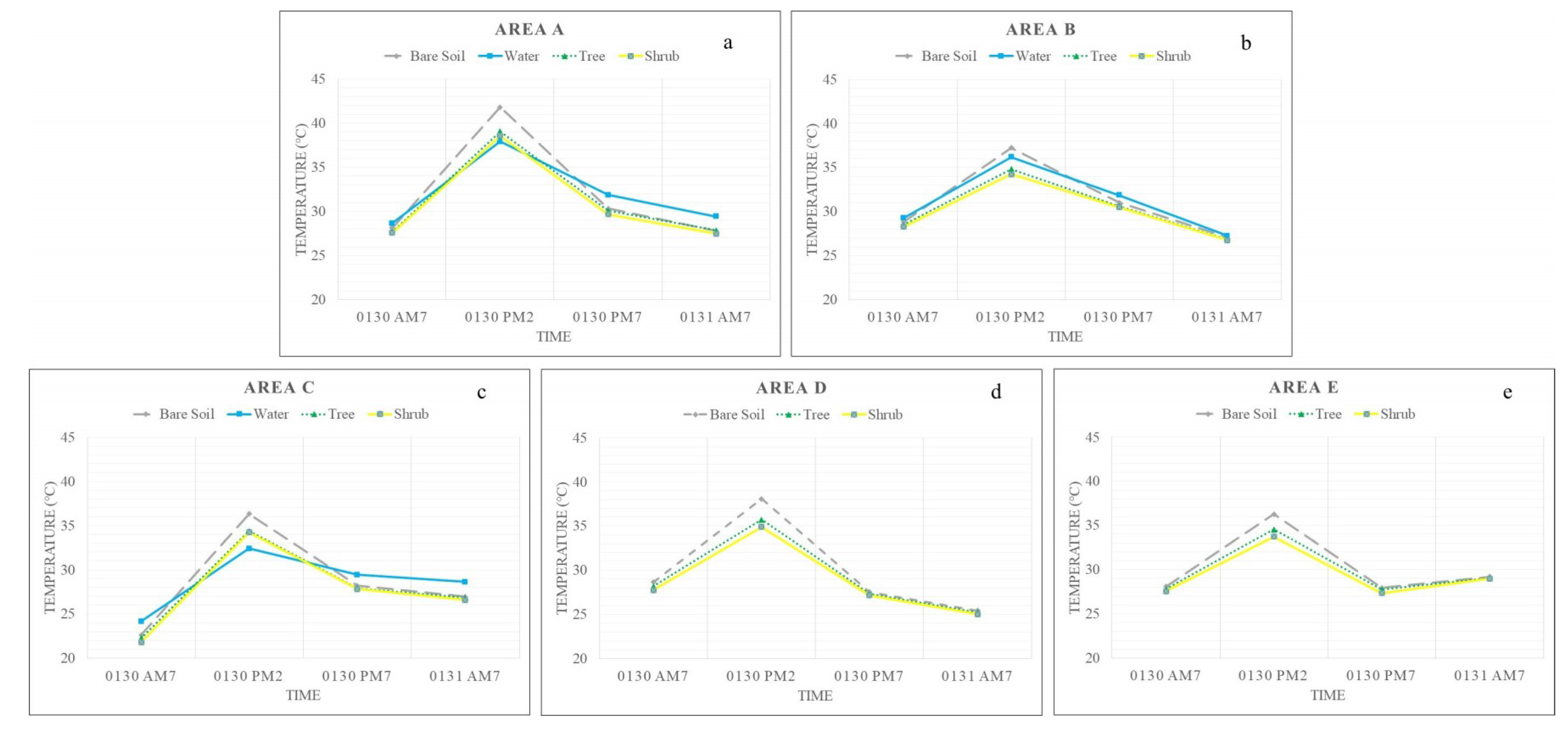
4.2. PCA and Spatial Characteristics of the Thermal Temperature
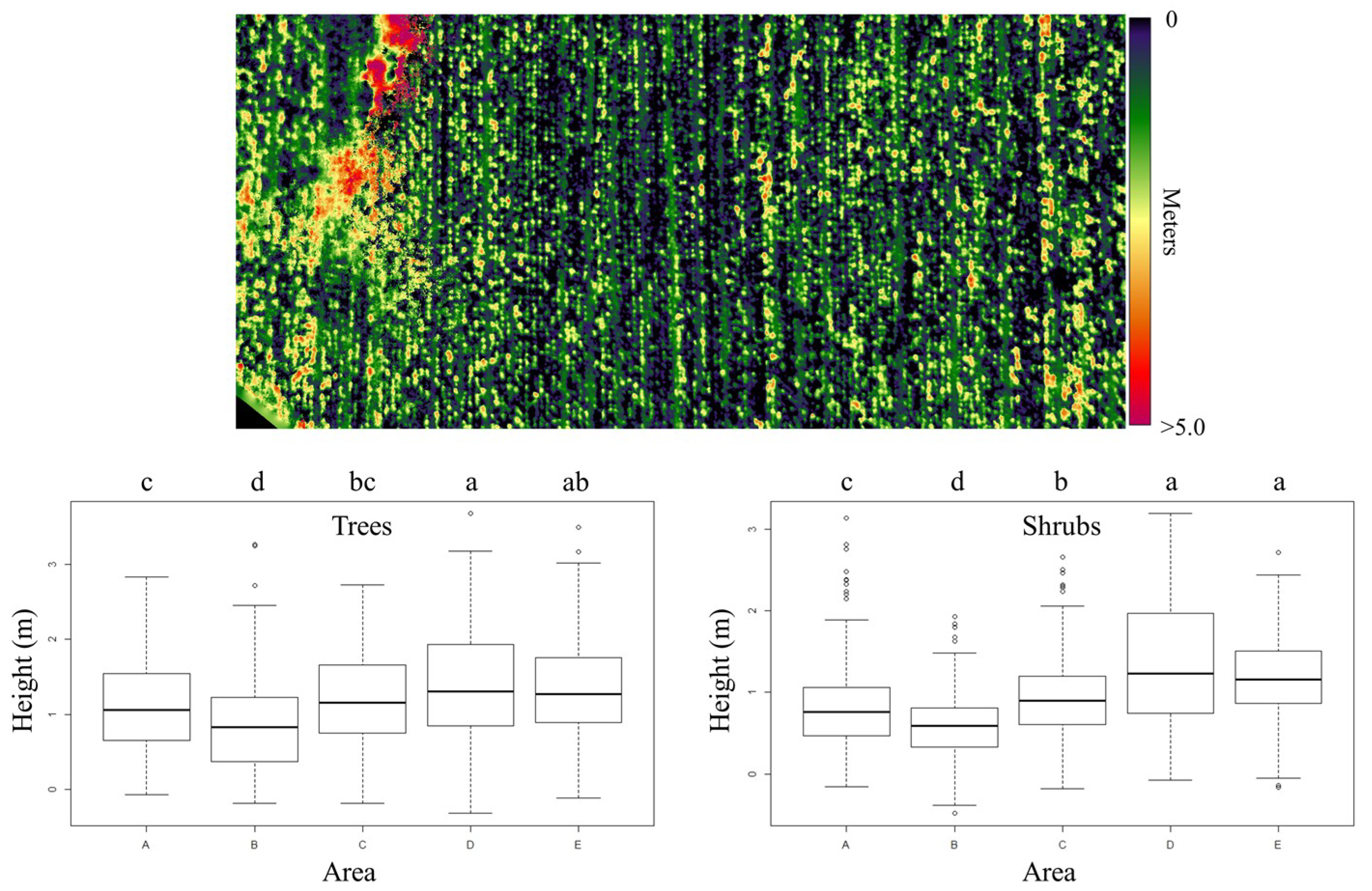
4.3. Tree Height-to-Area Characteristics
5. Discussion
5.1. Thermal Mapping
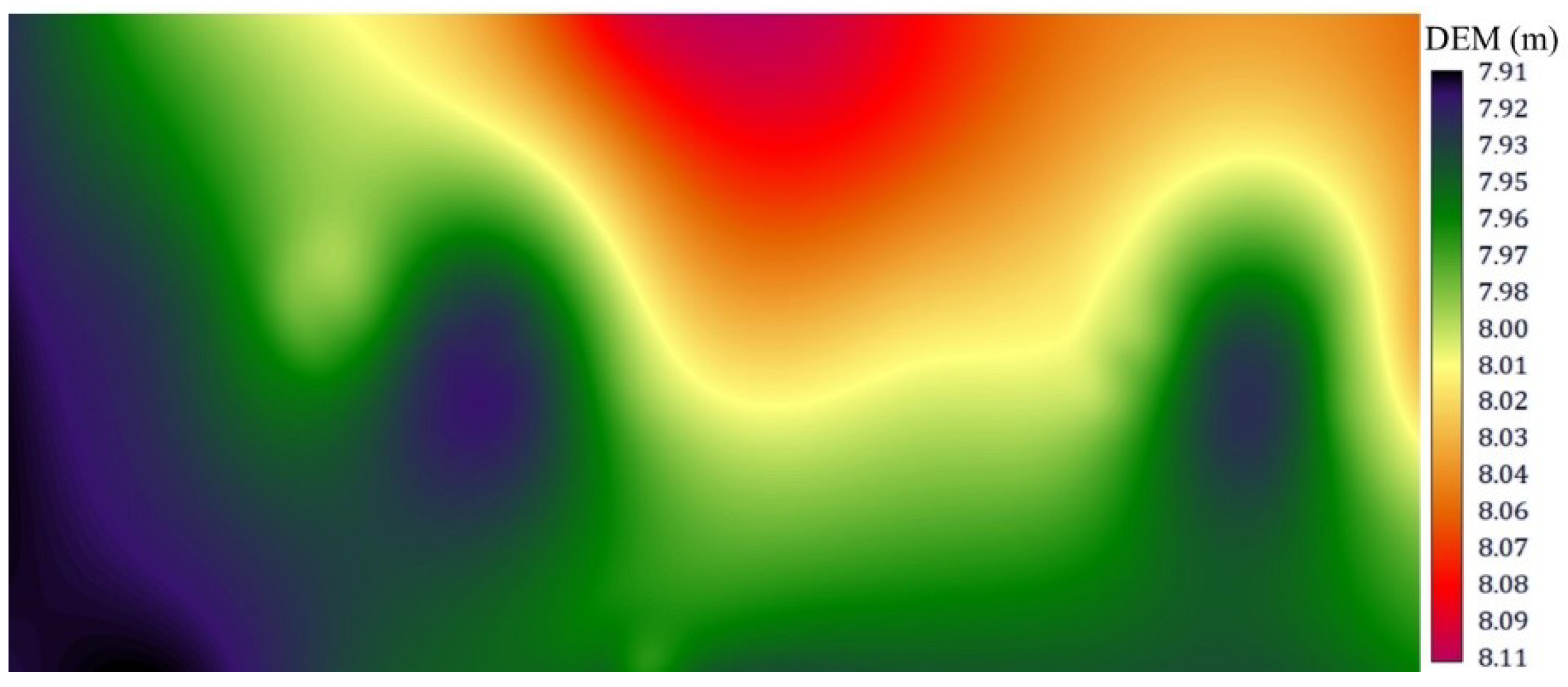
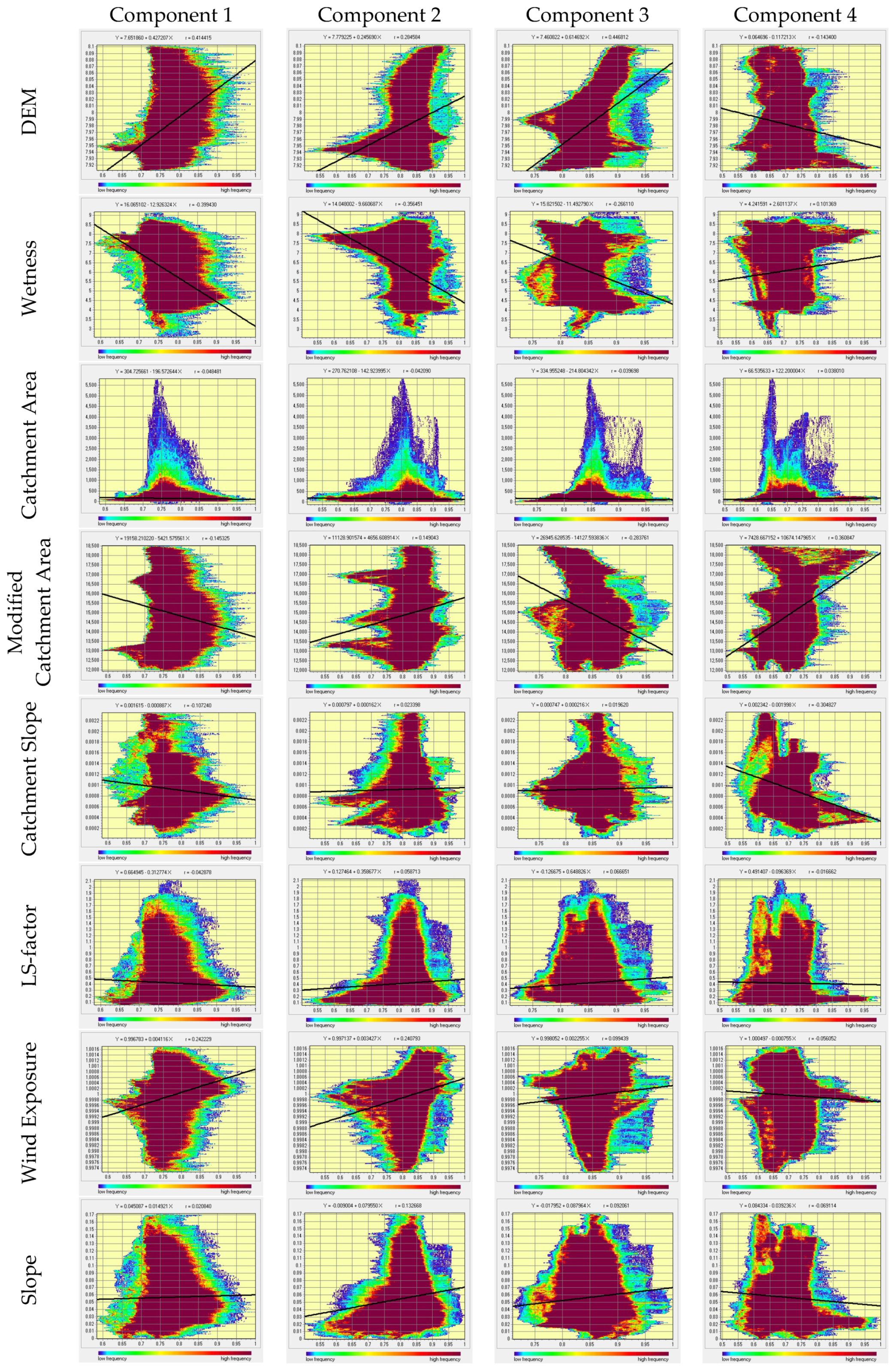
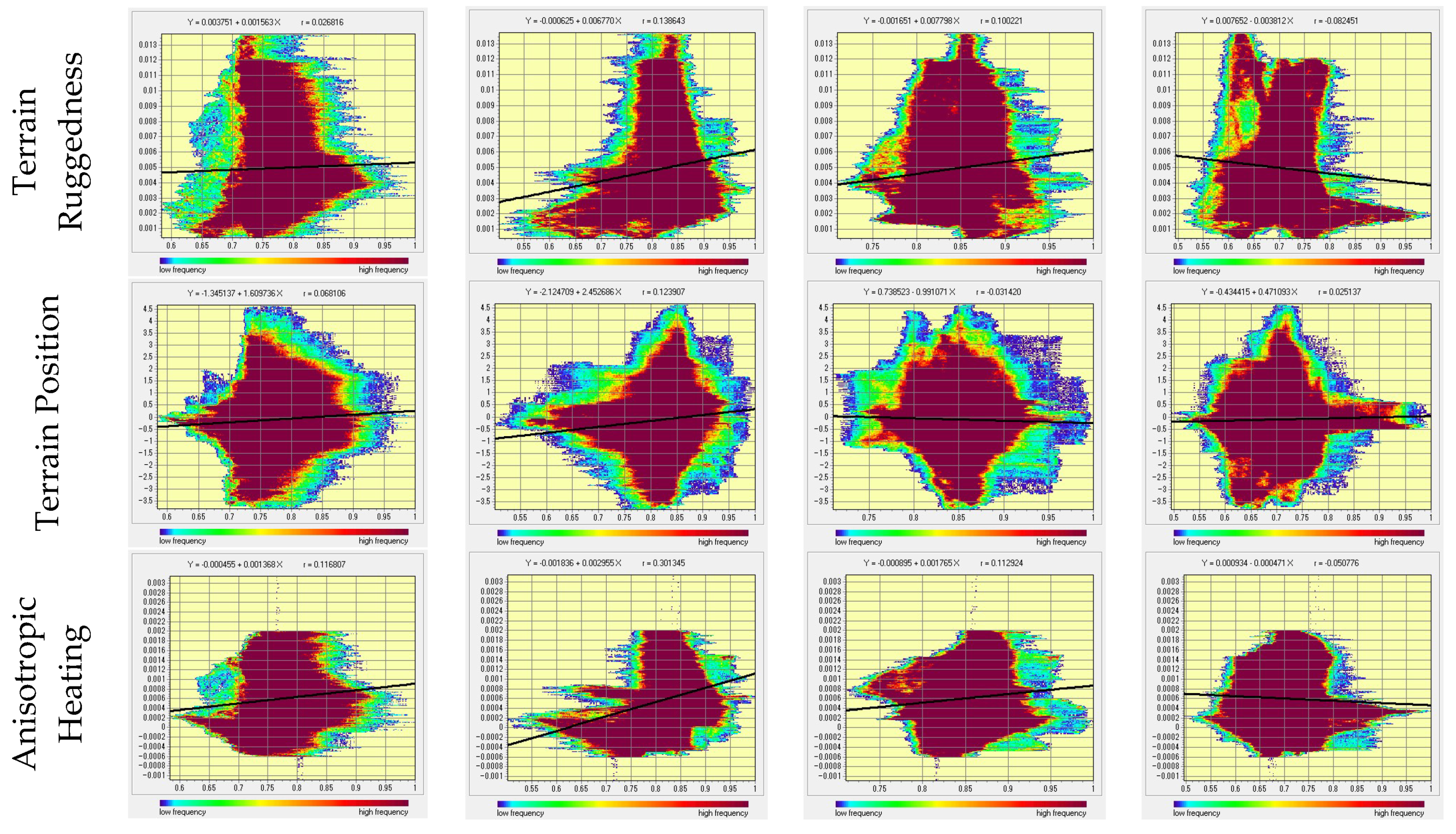
5.2. PCA Components Relating to Topographic Variables
6. Conclusions
Author Contributions
Funding
Acknowledgments
Conflicts of Interest
References
- Huijnen, V.; Wooster, M.J.; Kaiser, J.W.; Gaveau, D.L.A.; Flemming, J.; Parrington, M.; Inness, A.; Murdiyarso, D.; Main, B.; Van Weele, M. Fire carbon emissions over maritime southeast Asia in 2015 largest since 1997. Sci. Rep. 2016, 6, 26886. [Google Scholar] [CrossRef] [PubMed] [Green Version]
- Cattau, M.E.; Harrison, M.E.; Shinyo, I.; Tungau, S.; Uriarte, M.; DeFries, R. Sources of anthropogenic fire ignitions on the peat-swamp landscape in Kalimantan, Indonesia. Glob. Environ. Chang. 2016, 39, 205–219. [Google Scholar] [CrossRef]
- Sumarga, E. Spatial Indicators for Human Activities May Explain the 2015 Fire Hotspot Distribution in Central Kalimantan Indonesia. Trop. Conserv. Sci. 2017, 10. [Google Scholar] [CrossRef]
- Stockwell, C.E.; Jayarathne, T.; Cochrane, M.A.; Ryan, K.C.; Putra, E.I.; Saharjo, B.H.; Nurhayati, A.D.; Albar, I.; Blake, D.R.; Simpson, I.J.; et al. Field measurements of trace gases and aerosols emitted by peat fires in Central Kalimantan, Indonesia, during the 2015 El Niño. Atmos. Chem. Phys. 2016, 16, 11711–11732. [Google Scholar] [CrossRef]
- Hooijer, A.; Page, S.; Canadell, J.G.; Silvius, M.; Kwadijk, J.; Wösten, H.; Jauhiainen, J. Current and future CO2 emissions from drained peatlands in Southeast Asia. Biogeosciences 2010, 7, 1505–1514. [Google Scholar] [CrossRef]
- Ritzema, H.; Limin, S.; Kusin, K.; Jauhiainen, J.; Wösten, H. Canal blocking strategies for hydrological restoration of degraded tropical peatlands in Central Kalimantan, Indonesia. CATENA 2014, 114, 11–20. [Google Scholar] [CrossRef]
- Holden, J.; Wallage, Z.E.; Lane, S.N.; Mcdonald, A.T. Water table dynamics in undisturbed, drained and restored blanket peat. J. Hydrol. 2011, 302, 103–114. [Google Scholar] [CrossRef]
- Parry, L.E.; Holden, J.; Chapman, P.J. Restoration of blanket peatlands. J. Environ. Manag. 2014, 133, 193–205. [Google Scholar] [CrossRef] [PubMed] [Green Version]
- Jauhiainen, J.; Page, S.S.; Vasander, H. Greenhouse gas dynamics in degraded and restored tropical peatland. Mires Peat 2016, 17. [Google Scholar] [CrossRef]
- Hooijer, A.; Page, A.; Jauhiainen, J.; Lee, W.A.; Lu, X.X.; Idris, A.; Anshari, G. Subsidence and carbon loss in drained tropical peatlands. Biogeosciences 2012, 9, 1053–1071. [Google Scholar] [CrossRef] [Green Version]
- Jauhiainen, J.; Kerojoki, O.; Silvennoinen, H.; Limin, S.; Vasander, H. Heterotrophic respiration in drained tropical peat is greatly affected by temperature—A passive ecosystem cooling experiment. Environ. Res. Lett. 2014, 9, 105013. [Google Scholar] [CrossRef]
- Hilasvuori, E.; Akujärvi, A.; Fritze, H.; Karhu, K.; Laiho, R.; Mäkiranta, P.; Oinonen, M.; Palonen, V.; Vanhala, P.; Liski, J. Temperature sensitivity of decomposition in a peat profile. Soil Biol. Biochem. 2013, 67, 47–54. [Google Scholar] [CrossRef]
- Dennis, R.A.; Mayer, J.; Applegate, G.; Chokkalingam, U.; Colfer, C.J.P.; Kurniawan, I.; Lachowski, H.; Maus, P.; Permana, R.P.; Ruchiat, Y.; et al. Fire, People and Pixels: Linking Social Science and Remote Sensing to Understand Underlying Causes and Impacts of Fires in Indonesia. Hum. Ecol. 2005, 33, 465–504. [Google Scholar] [CrossRef]
- Fuller, D.O.; Hardiono, M.; Meijaard, E. Deforestation projections for carbon-rich peat swamp forests of Central Kalimantan, Indonesia. Environ. Manag. 2011, 48, 436–447. [Google Scholar] [CrossRef] [PubMed]
- Atwood, E.C.; Englhart, S.; Lorenz, E.; Halle, W.; Wiedemann, W.; Siegert, F. Detection and Characterization of Low Temperature Peat Fires during the 2015 Fire Catastrophe in Indonesia Using a New High-Sensitivity Fire Monitoring Satellite Sensor (FireBird). PLoS ONE 2016, 11, e0159410. [Google Scholar] [CrossRef] [PubMed]
- Sholihah, R.I.; Trisasongko, B.H.; Shiddiq, D.; La Ode, S.I.; Kusdaryanto, S.; Manijo; Panuju, D.R. Identification of Agricultural Drought Extent Based on Vegetation Health Indices of Landsat Data: Case of Subang and Karawang, Indonesia. Procedia Environ. Sci. 2016, 33, 14–20. [Google Scholar] [CrossRef]
- Liu, G.; Zhang, Q.; Li, G.; Doronzo, D.M. Response of land cover types to land surface temperature derived from Landsat-5 TM in Nanjing Metropolitan Region, China. Environ. Earth Sci. 2016, 75, 1386. [Google Scholar] [CrossRef]
- Leng, L.Y.; Ahmed, O.H.; Jalloh, M.B. Brief review on climate change and tropical peatlands. Geosci. Front. 2018, in press. [Google Scholar] [CrossRef]
- Davidson, E.A.; Janssens, I.A. Temperature sensitivity of soil carbon decomposition and feedbacks to climate change. Nature 2006, 440, 165–173. [Google Scholar] [CrossRef] [PubMed] [Green Version]
- Iizuka, K.; Yonehara, T.; Itoh, M.; Kosugi, Y. Estimating Tree Height and Diameter at Breast Height (DBH) from Digital Surface Models and Orthophotos Obtained with an Unmanned Aerial System for a Japanese Cypress (Chamaecyparis obtusa) Forest. Remote Sens. 2018, 10, 13. [Google Scholar] [CrossRef]
- Jaud, M.; Passot, S.; Le Bivic, R.; Delacourt, C.; Grandjean, P.; Le Dantec, N. Assessing the Accuracy of High Resolution Digital Surface Models Computed by PhotoScan® and MicMac® in Sub-Optimal Survey Conditions. Remote Sens. 2016, 8, 465. [Google Scholar] [CrossRef]
- Luna, I.; Lobo, A. Mapping Crop Planting Quality in Sugarcane from UAV Imagery: A Pilot Study in Nicaragua. Remote Sens. 2016, 8, 500. [Google Scholar] [CrossRef]
- Iizuka, K.; Itoh, M.; Shiodera, S.; Matsubara, M.; Dohar, M.; Watanabe, K. Advantages of unmanned aerial vehicle (UAV) photogrammetry for landscape analysis compared with satellite data: A case study of postmining sites in Indonesia. Cogent Geosci. 2018, 4, 1498180. [Google Scholar] [CrossRef]
- Flynn, K.F.; Chapra, S.C. Remote sensing of submerged aquatic vegetation in a shallow non-turbid river using an unmanned aerial vehicle. Remote Sens. 2014, 6, 12815–12836. [Google Scholar] [CrossRef]
- Aghaei, M.; Gandelli, A.; Grimaccia, F.; Leva, S.; Zich, R.E. IR real-time analyses for PV system monitoring by digital image processing techniques. In Proceedings of the International Conference on Event-based Control Communication and Signal Processing (EBCCSP), Krakow, Poland, 17–19 June 2015; pp. 1–6. [Google Scholar]
- Gonzalez, L.F.; Montes, G.A.; Puig, E.; Johnson, S.; Mengersen, K.; Gaston, K.J. Unmanned Aerial Vehicles (UAVs) and Artificial Intelligence Revolutionizing Wildlife Monitoring and Conservation. Sensors 2016, 16, 97. [Google Scholar] [CrossRef] [PubMed] [Green Version]
- Hare, D.K.; Boutt, D.F.; Clement, W.P.; Hatch, C.E.; Davenport, G.; Hackman, A. Hydrogeological controls on spatial patterns of groundwater discharge in peatlands. Hydrol. Earth Syst. Sci. 2017, 21, 6031–6048. [Google Scholar] [CrossRef] [Green Version]
- Maes, W.H.; Huete, A.R.; Steppe, K. Optimizing the Processing of UAV-Based Thermal Imagery. Remote Sens. 2017, 9, 476. [Google Scholar] [CrossRef]
- Guerra-Hernández, J.; González-Ferreiro, E.; Monleón, V.J.; Faias, S.P.; Tomé, M.; Díaz-Varela, R.A. Use of Multi-Temporal UAV-Derived Imagery for Estimating Individual Tree Growth in Pinus pinea Stands. Forests 2017, 8, 300. [Google Scholar] [CrossRef]
- Motohka, T.; Nasahara, K.N.; Oguma, H.; Tsuchida, S. Applicability of Green-Red Vegetation Index for Remote Sensing of Vegetation Phenology. Remote Sens. 2010, 2, 2369–2387. [Google Scholar] [CrossRef] [Green Version]
- Ma, H.; Qin, Q.; Shen, X. Shadow segmentation and compensation in high resolution satellite images. In Proceedings of the 2008 IEEE International Geoscience and Remote Sensing Symposium, Boston, MA, USA, 7–11 July 2008; Volume 2, pp. 1036–1039. [Google Scholar]
- Riccioli, F.; El Asmar, T.; El Asmar, J.P.; Fagarazzi, C.; Casini, L. Artificial neural network for multifunctional areas. Environ. Monit. Assess. 2016, 188, 67. [Google Scholar] [CrossRef] [PubMed]
- Tang, F.; Xu, H. Impervious Surface Information Extraction Based on Hyperspectral Remote Sensing Imagery. Remote Sens. 2017, 9, 550. [Google Scholar] [CrossRef]
- Westra, S.; Brown, C.; Lall, U.; Koch, I.; Sharma, A. Interpreting variability in global SST data using independent component analysis and principal component analysis. Int. J. Clim. 2010, 30, 333–346. [Google Scholar] [CrossRef]
- Barreira, S.; Compagnucci, R. Spatial fields of Antarctic sea-ice concentration anomalies for summer–autumn and their relationship to Southern Hemisphere atmospheric circulation during the period 1979–2009. Ann. Glaciol. 2011, 52, 140–150. [Google Scholar] [CrossRef]
- Ahmed, B.; Kamruzzaman, M.; Zhu, X.; Rahman, M.S.; Choi, K. Simulating Land Cover Changes and Their Impacts on Land Surface Temperature in Dhaka, Bangladesh. Remote Sens. 2013, 5, 5969–5998. [Google Scholar] [CrossRef] [Green Version]
- Conrad, O.; Bechtel, B.; Bock, M.; Dietrich, H.; Fischer, E.; Gerlitz, L.; Wehberg, J.; Wichmann, V.; Böhner, J. System for Automated Geoscientific Analyses (SAGA) v. 2.1.4. Geosci. Model Dev. Discuss. 2015, 8, 2271–2312. [Google Scholar] [CrossRef]
- Kim, Y.M.; You, K.P.; You, J.Y. Characteristics of Wind Velocity and Temperature Change near an Escarpment-Shaped Road Embankment. Sci. World J. 2014, 2014, 695629. [Google Scholar] [CrossRef] [PubMed]
- Al-Kayssi, A.W.; Al-Karaghouli, A.A.; Hasson, A.M.; Beker, S.A. Influence of soil moisture content on soil temperature and heat storage under greenhouse conditions. J. Agric. Eng. Res. 1990, 45, 241–252. [Google Scholar] [CrossRef]
- Lakshmi, V.; Jackson, T.J.; Zehrfuhs, D. Soil moisture-temperature relationships: Results from two field experiments. Hydrol. Process. 2003, 17, 3041–3057. [Google Scholar] [CrossRef]


| Reference Class | Bare | Water | Tree | Shrub | Shadow | Total | Error Commission | |
|---|---|---|---|---|---|---|---|---|
| Classified Class | ||||||||
| Bare | 285 | 4 | 4 | 293 | 0.027 | |||
| Water | 288 | 288 | 0 | |||||
| Tree | 9 | 282 | 7 | 298 | 0.054 | |||
| Shrub | 2 | 14 | 293 | 309 | 0.052 | |||
| Shadow | 4 | 8 | ||||||
| Total | 300 | 300 | 300 | 300 | 1200 | |||
| Error Omission | 0.05 | 0.04 | 0.06 | 0.023 | 95.67% | |||
© 2018 by the authors. Licensee MDPI, Basel, Switzerland. This article is an open access article distributed under the terms and conditions of the Creative Commons Attribution (CC BY) license (http://creativecommons.org/licenses/by/4.0/).
Share and Cite
Iizuka, K.; Watanabe, K.; Kato, T.; Putri, N.A.; Silsigia, S.; Kameoka, T.; Kozan, O. Visualizing the Spatiotemporal Trends of Thermal Characteristics in a Peatland Plantation Forest in Indonesia: Pilot Test Using Unmanned Aerial Systems (UASs). Remote Sens. 2018, 10, 1345. https://0-doi-org.brum.beds.ac.uk/10.3390/rs10091345
Iizuka K, Watanabe K, Kato T, Putri NA, Silsigia S, Kameoka T, Kozan O. Visualizing the Spatiotemporal Trends of Thermal Characteristics in a Peatland Plantation Forest in Indonesia: Pilot Test Using Unmanned Aerial Systems (UASs). Remote Sensing. 2018; 10(9):1345. https://0-doi-org.brum.beds.ac.uk/10.3390/rs10091345
Chicago/Turabian StyleIizuka, Kotaro, Kazuo Watanabe, Tsuyoshi Kato, Niken Andika Putri, Sisva Silsigia, Taishin Kameoka, and Osamu Kozan. 2018. "Visualizing the Spatiotemporal Trends of Thermal Characteristics in a Peatland Plantation Forest in Indonesia: Pilot Test Using Unmanned Aerial Systems (UASs)" Remote Sensing 10, no. 9: 1345. https://0-doi-org.brum.beds.ac.uk/10.3390/rs10091345