RDCRMG: A Raster Dataset Clean & Reconstitution Multi-Grid Architecture for Remote Sensing Monitoring of Vegetation Dryness

Abstract

In recent years, remote sensing (RS) research on crop growth status monitoring has gradually turned from static spectrum information retrieval in large-scale to meso-scale or micro-scale, timely multi-source data cooperative analysis; this change has presented higher requirements for RS data acquisition and analysis efficiency. How to implement rapid and stable massive RS data extraction and analysis becomes a serious problem. This paper reports on a Raster Dataset Clean & Reconstitution Multi-Grid (RDCRMG) architecture for remote sensing monitoring of vegetation dryness in which different types of raster datasets have been partitioned, organized and systematically applied. First, raster images have been subdivided into several independent blocks and distributed for storage in different data nodes by using the multi-grid as a consistent partition unit. Second, the “no metadata model” ideology has been referenced so that targets raster data can be speedily extracted by directly calculating the data storage path without retrieving metadata records; third, grids that cover the query range can be easily assessed. This assessment allows the query task to be easily split into several sub-tasks and executed in parallel by grouping these grids. Our RDCRMG-based change detection of the spectral reflectance information test and the data extraction efficiency comparative test shows that the RDCRMG is reliable for vegetation dryness monitoring with a slight reflectance information distortion and consistent percentage histograms. Furthermore, the RDCGMG-based data extraction in parallel circumstances has the advantages of high efficiency and excellent stability compared to that of the RDCGMG-based data extraction in serial circumstances and traditional data extraction. At last, an RDCRMG-based vegetation dryness monitoring platform (VDMP) has been constructed to apply RS data inversion in vegetation dryness monitoring. Through actual applications, the RDCRMG architecture is proven to be appropriate for timely vegetation dryness RS automatic monitoring with better performance, more reliability and higher extensibility. Our future works will focus on integrating more kinds of continuously updated RS data into the RDCRMG-based VDMP and integrating more multi-source datasets based collaborative analysis models for agricultural monitoring.

1. Introduction

In Recent years, with the increase of Multi-Source Remote Sensing (RS) Data, RS research on crop growth status monitoring (including crop classification [1,2,3], crop yield estimation [4,5,6,7,8], and crop leaf area index analysis [9,10]) has gradually turned from static spectrum information retrieval in large-scale to meso-scale or micro-scale, near real-time multi-source data cooperative analysis; this change has presented higher requirements for RS data acquisition and analysis efficiency. Since RS data has the characteristics of large size, numerous formats, various temporal-spatial resolutions and a complicated pretreatment process, how to implement rapid and stable massive RS data extraction and analysis becomes a serious problem.

The traditional spatial information system has problems with multi-source RS data applications. For most RS data center systems (e.g., China Resources Satellite Application Center, National Aeronautics and Space Administration Earth Observing System, and Google Earth), efficient RS data storage, retrieval and sharing have been realized by applying technologies such as NOSQL (Not Only Structured Query Language), Massive Distributed Storage, Parallel Computation, and Multistage Tile Maps. However, since RS datasets have been separately stored and have differences in the map framing rule and spatial coordinate system, these systems may not be appropriate for vegetation dryness monitoring. First, the dryness information acutely changes, and requires the relevant multisource time-series RS data to be quickly extracted; second, the monitoring objects are discretely distributed in thousands of various sized land masses, and extracting RS data according to an enveloping rectangle of monitoring objects may arouse large data redundancy and decrease the efficiency. In conclusion, it is important to construct a consistent data organization structure, by which different types of RS data that covers assigned monitoring areas can be speedily extracted.

The geographical grid runs a long course from a remote source and shows innate advantages for constructing consistent spatial data organizational structures by its theoretical “divide and rule” and “implicit position information” connotations. Many studies indicate that using some grid system (such as a rectangular grid or meridian/parallel line) divides the research region into several local blocks and treats blocks as basic units to represent a region’s corresponding attributes, categories, parameters and virtual reality, will have good applicability in spatial big data storage, management, integration, calculation and presentation. Generally, we should analyze practical applications to define applicable grid system, which can be divided into the four classes: regular polyhedron-based grid system: the sphere VORONOI-based grid system, the longitude/latitude line-based grid system and the planar projection-based grid system, according to space benchmark.

For the regular polyhedron-based grid system, platonic polyhedrons (tetrahedrons, cube, octahedron, dodecahedron, and icosahedrons) have been embedded in the Earth as nuclear structures whose vertices have been projected onto the Earth’s surface; lines of proximal vertices constitute polygon sets that cover the whole surface, and on these bases, geometric structures with multi-layer, multi-resolution and global characteristics have been constructed by subdividing each polygon layer by layer [11,12,13,14]. In 1990, Fekete presented the Sphere Quadtrees (SQT) model that constructs a triangular grid base on a spherical arc, which expresses straightforward geometrical significance and balanced projection distortion but has problems transforming coordinates [15,16]. In 1989, the Snyder Equal-Area Polyhedral projection (SEA) was presented; grids were divided based on each surface of the polyhedron and then projected onto the Earth’s surface. However, the SEA has low efficiency in data transformation [17]. Dutton described the Octahedral Quaternary Triangular Mesh (O-QTM) for positional data descriptions, which takes shape as a regular hierarchical triangulation of an octahedron embedded in a planet; it densifies four child triangles developed within each existing one, and each has a unique numeric address [18,19]. Zhou et al. proposed a new pole-oriented DGGS (the Quaternary Quadrangle Mesh (QQM)) that uses semi-hexagon (a type of quadrangle) grids in the polar regions and rectangular grids elsewhere [20]. Despite their advantages of balanced projection deformation, regular shape, isotropy, and uniformity, the regular polyhedron-based grid systems are generally inefficient in data management, conversion and integration. In most cases, the grid shape is not applicable for matrix structure-based RS data.

The grid partition method of the sphere VORONOI-based grid system is similar to the planar VORONOI graph. Points have been assigned to grids based on the minimum distance to each grid center so that the structure is dynamically stable and can dynamically update the local data. Lukatela build terrain TIN model that is based on the VORONOI grid and can complete global visual modeling [21]; Wang et al. presented a QTM model-based sphere VORONOI algorithm to improve grid construction efficiency in high-level conditions [22]. However, there is no nested relationship between grids of adjacent layers; therefore, it is difficult for multi-scale RS data correlation.

The longitude/latitude -based grid system divides the total study area into several local blocks in accordance with equal (or unequal) longitude/latitude differences and has been widely used in RS data retrieval [23,24,25,26,27]; it has low computational complexity, is convenient for multi-level grid subdivisions, seamlessly integrates adjacent grids, possesses a concise index structure. However, since the grid area and shape are influenced by the spheroid, they change significantly with the latitude, and it is difficult to keep a consistent area for each grid. With RS images that cover grids with the same longitude/latitude differences, their coverage area and spatial resolution (unit: degree) may be different. Therefore, this grid system is not appropriate for a consistent RS data partitioning reference. Although some studies construct grid areas to be approximately equal by adjusting the grid longitude/latitude difference with the changing latitude [28,29], the complexity of the grid structure has been increased, and the morphing is still inevitable.

According to planar projection-based grid system, the research area has been projected to a planar coordinate system and subdivided by km grids. This grid system has been integrated into many national standard grid systems (including the United States National Grid and the China National Geographic Grid) with the characteristics of a clear spatial mathematical foundation, a comprehensible partition rule, a simple conversion algorithm between the grid code and spatial coordinates, a consistent grid area/shape at the same scale, good compatibility with RS data organization and transformation, high flexibility for different types of RS data with different spatial resolutions (unit: meter) and map framing rule. However, to control the transformation error between the planar grid and the real Earth surface, the strip division projection method has been used, and it cannot be seamlessly integrated between grids constructed based on adjacent projection zones.

This paper reports on a Raster Dataset Clean & Reconstitution Multi-Grid (RDCRMG) architecture for remote sensing monitoring of vegetation dryness, by which different types of raster datasets have been partitioned, consistently organized and systematically applied. On the one hand, raster images have been subdivided into several independent blocks and distributed stored in different data nodes by using multi-grid as consistent partition unit, meanwhile adjacent blocks have been distributed to the same data node; on the other hand, a “no metadata model” ideology has been referenced, so that target raster data can be speedy extracted by directly calculate the data store path base on spatial query conditions without retrieving metadata records; thirdly, grids that cover the query range can be easily figured out, thereby the query task can be easily split into several sub-tasks and executed in parallel by grouping these grids. Our experiments on raster data extraction efficiency and pixel value change detection base on GF-1 RS data demonstrate that the RDCRMG architecture is comparatively efficient and stable for raster data extraction. Furthermore, a prototype system has been constructed and applied to actual vegetation dryness to test the practicality of the RDCRMG architecture.

The remainder of the article is organized as follows. Section 2 provides the details of the RDCRMG architecture, including its design principles, spatial references, grid partition, coding strategy, and data retrieval strategy. Section 3 reports on the change detection of the spectral reflectance information test and the data extraction efficiency comparative test using the RDCRMG architecture with the GF-1 RS data. Section 4 presents the application of the RDCRMG architecture on vegetation dryness monitoring. Finally, Section 5 and Section 6 discusses the results and concludes this study.

2. Multi-Grid Architecture Design Method

2.1. Design Target and Principles

The goal of the RDCRMG architecture is to provide a consistent multi-source RS data organization, storage, retrieval and analysis rule for meso-scale or micro-scale crop status monitoring in the whole region of China; this goal would allow different types of RS data that cover assigned monitoring area to be speedily extracted and calculated. In terms of data organization, aimed at the problem of various framing units and lacking uniform segmentation criteria and positional correspondence, RS data should be subdivided into several inerratic blocks with the same data format based on the consistent grid standard. In terms of data storage, aimed at spectrum computing requirements of remote sensing monitoring, inerratic data blocks have been stored in different grid scales according to its spatial resolution, and the reflectivity characteristics of different bands should be maintained. In terms of data retrieval, spatial relationships between grid vertex geographic coordinates and pixel row/column numbers of data blocks should be constructed so that the corresponding grid code and storage path of data blocks can be rapidly calculated according to spatial-temporal query conditions. In terms of data analysis, the grid should be treated as a remote sensing inversion calculation element. Therefore, the whole task can be distributed to different grids and executed in parallel to increase calculation efficiency.

Since a multi-grid architecture has been proposed, a corresponding construction principle and application condition should be considered. In 1994, Goodchild presented a grid evaluation standard based on systematic global grid system research [30]; Kimerling supplemented the standard, and Clarke synthetically analyzed the abovementioned standard [31,32]. According to their research achievements, the grid area/shape similarity degree, the multi-scale hierarchical structure, the transfer approach relative to spatial coordinates, universality, and the degree of recognition can be treated as general requirements for global discrete grid system. Li et al. [24,25,26,27] stated that the global discrete grid system is appropriate for establishing the spatial information orientation and spatial retrieval mechanism; he then proposed the spatial information multi-grid (SIMG) for the integrated management of spatial data with diverse coordinated systems and defined the corresponding partitioning principles. Cheng et al. proposed geographic coordinate subdivision grid with one dimension-integral coding on 2n-tree (GeoSOT) for remote sensing data management [33,34,35]. Lewis et al. proposed Australian Geoscience Data Cube (AGDC) architecture for RS big data management and application [36].

Based on abovementioned studies, we propose the RDCRMG design principles as follows:

• The RDCRMG has a multi-leveled grid structure with a rigorous nested relationship and can be applied to multi-spatial resolution raster data storage.
• The RDCRMG contains an efficient coding scheme.
• The positional correspondence of adjacent level grids can be calculated by a simple linear formula.
• Grids at the same level have inerratic grid shapes with consistent areas and can be applied to the raster data model.
• Grids at the same level have simple positional relationships with each other.
• Spatial-temporal query conditions can be converted to data paths through a simple numerical method.
• The grid structures have good compatibility with the universal spatial data organization mode.
• The grid partitioning and encoding strategy has good universality and can be conveniently integrated with other grid systems or applications.
• The grid partitioning strategy is appropriate for data-intensive computing.

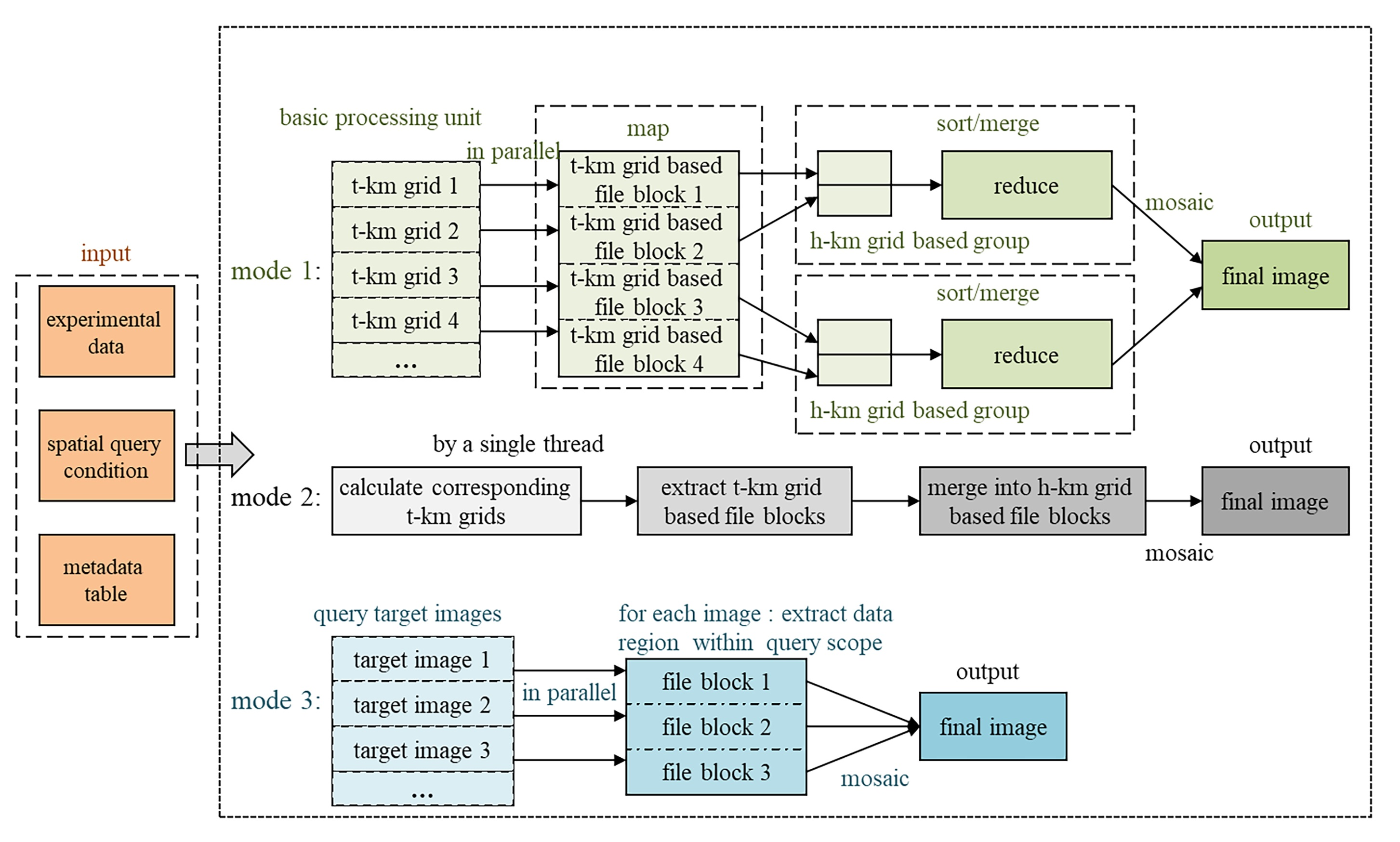
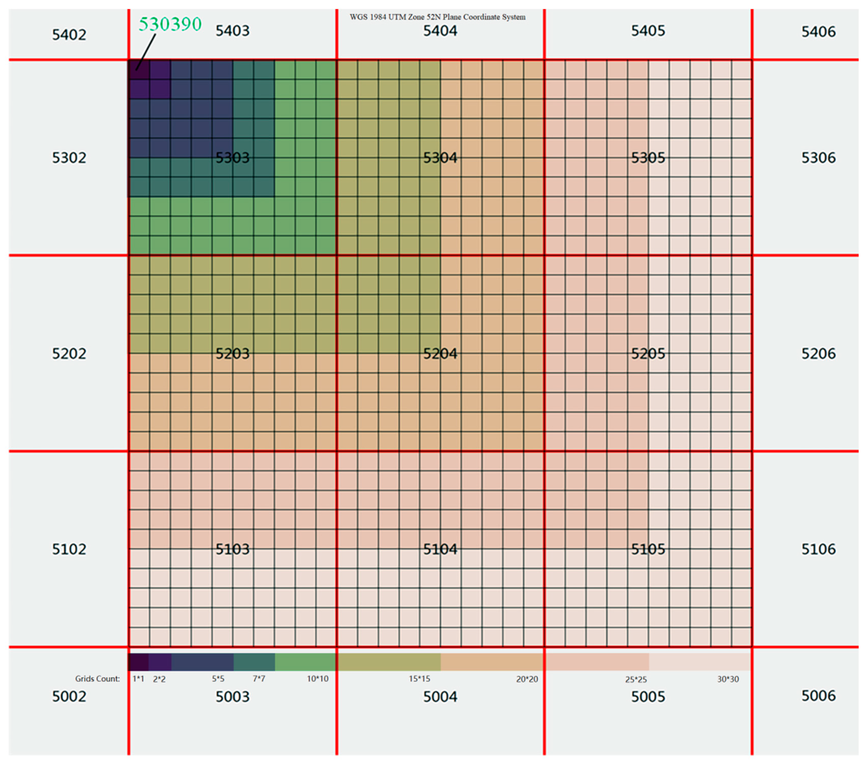
2.2. Multi-Grid Spatial Reference

The World Geodetic System 1984 (WGS 84)-based Universal Transverse Mercator (UTM) 6-degree strip division projection coordinate system has been designated as the RDCRMG spatial reference for uniform raster data organization and analysis.

First, compared with the regular polyhedron-based spatial reference, the WGS 84 UTM coordinate system has slightly inferior homogeneity, but it has better compatibility with the RS data matrix structure and map framing rule. Furthermore, the data management efficiency can be significantly increased with its clear spatial mathematical foundation, comprehensible partitioning rule and simple conversion algorithm between the grid code and spatial coordinates.

Second, compared with longitude/latitude line-based spatial reference, the WGS 84 UTM coordinate system has disadvantages with spatial continuity. Grids that cover different projection zones cannot be seamlessly integrated. However, it has a better “homolographic effect”, and the same type of RS data can be subdivided with a consistent spatial resolution (unit: meter).

Third, the WGS 84 UTM coordinate system has been widely used as an original RS data spatial reference. The information loss from the RS data partition and transformation process can be largely reduced by designing it as the RDCRMG spatial reference. Compared with conical or azimuthal projection, UTM projection is more accurate (projection error is within ±0.005%) in wider areas using strip division. When compared with the tangent cylindrical projection (the Gauss-Kruger projection), the error distribution of the UTM projection is more uniform, and corresponding pixels in projection zone boundary have less distortion.

Furthermore, it is known that the strip division projection method of the WGS 84 UTM coordinate system may break RS data spatial continuity and increase computation complexity. However, according to the data-intensive computing feature of the vegetation dryness monitoring-oriented RS inversion algorithm, the data clipping operation will hardly influence the calculation process and results (relevant experiments been reported in Section 3), and the computation speed will not be decreased by using grid-based parallel computing.

Lastly, the WGS 84 UTM coordinate system only works for data organization and spatial reference analysis. With respect to spatial visualization, partitioned calculation result data should be transformed into the WGS 84 Geographic Coordinate System for seamless data integration.

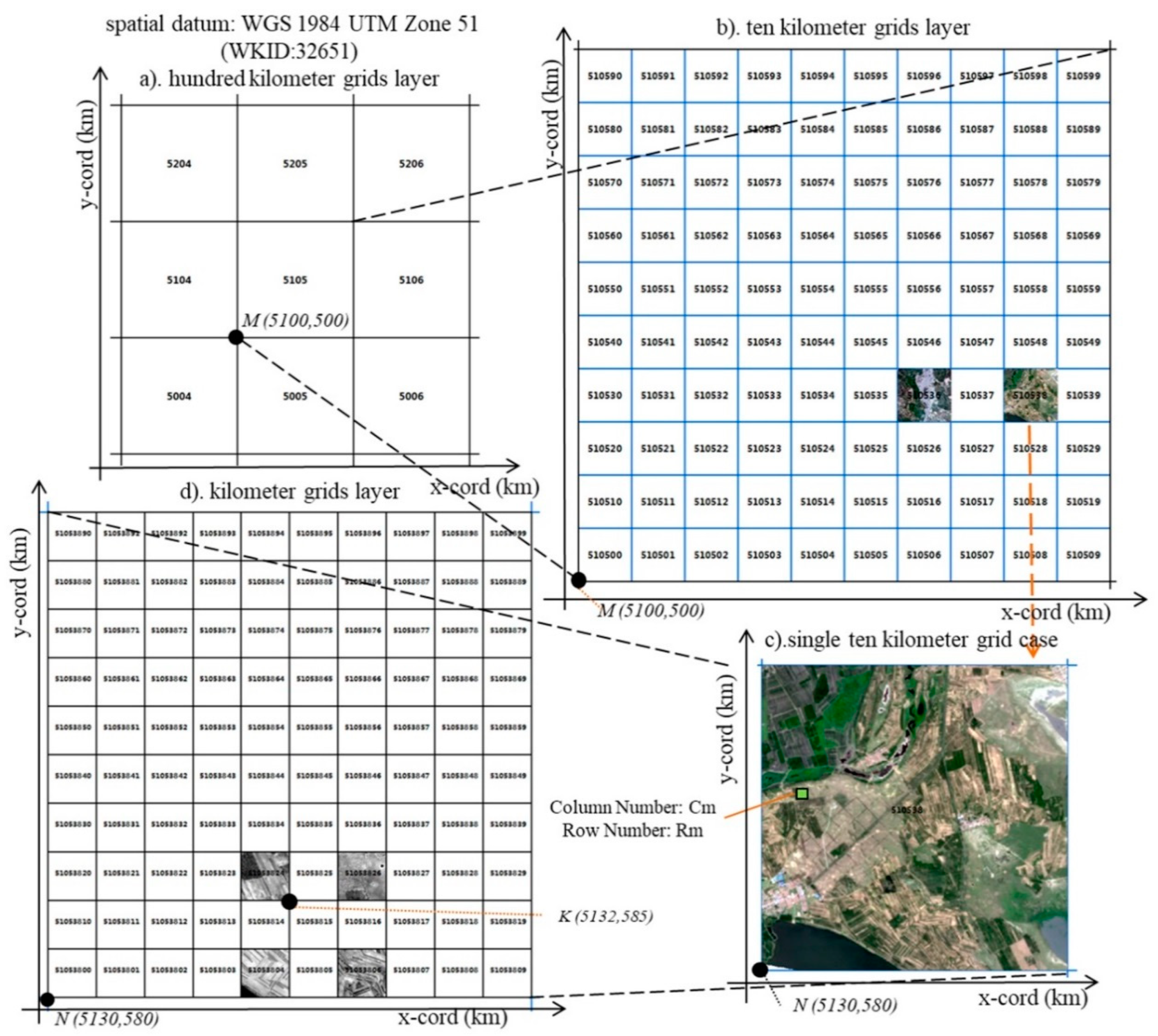
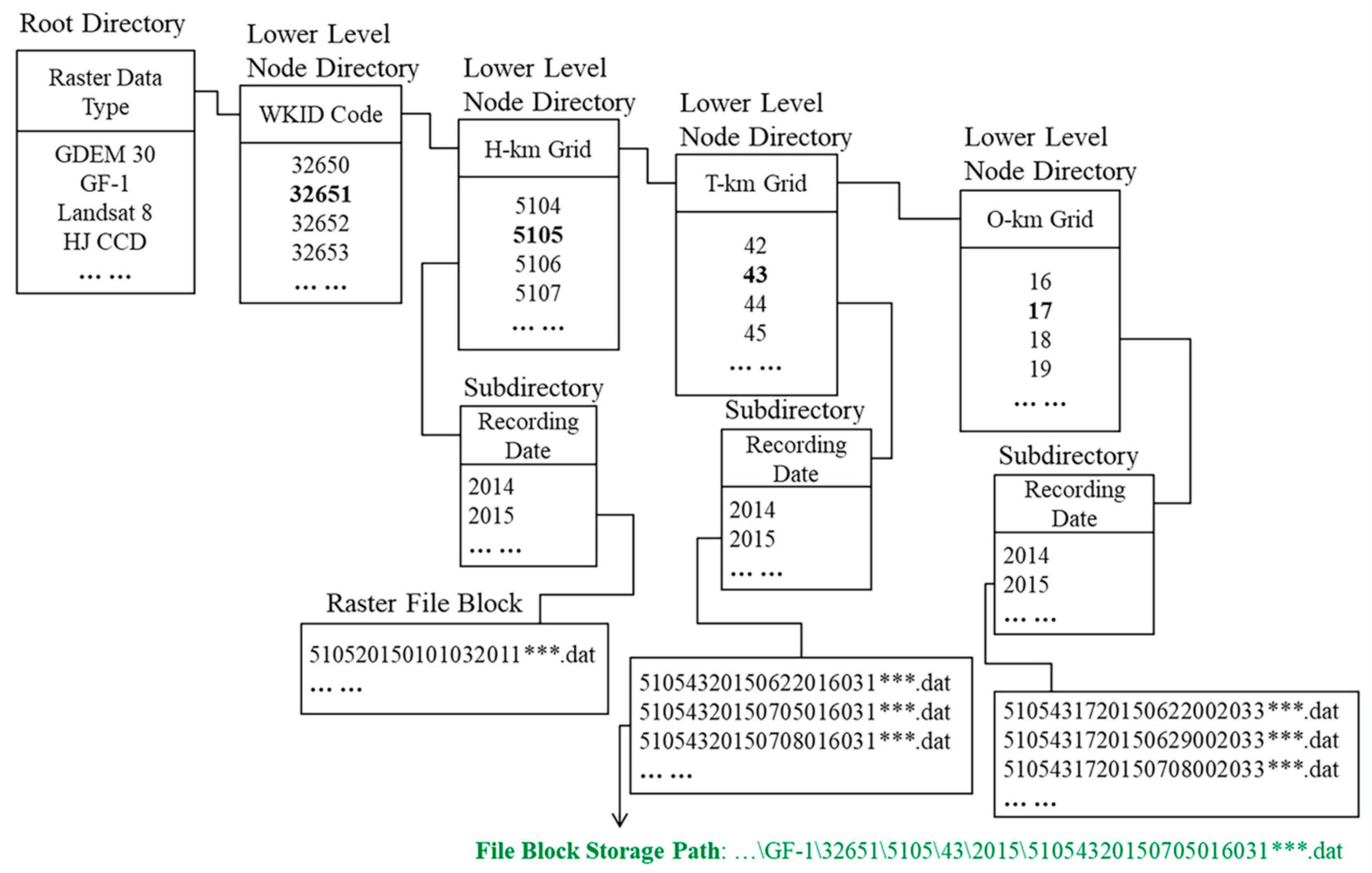
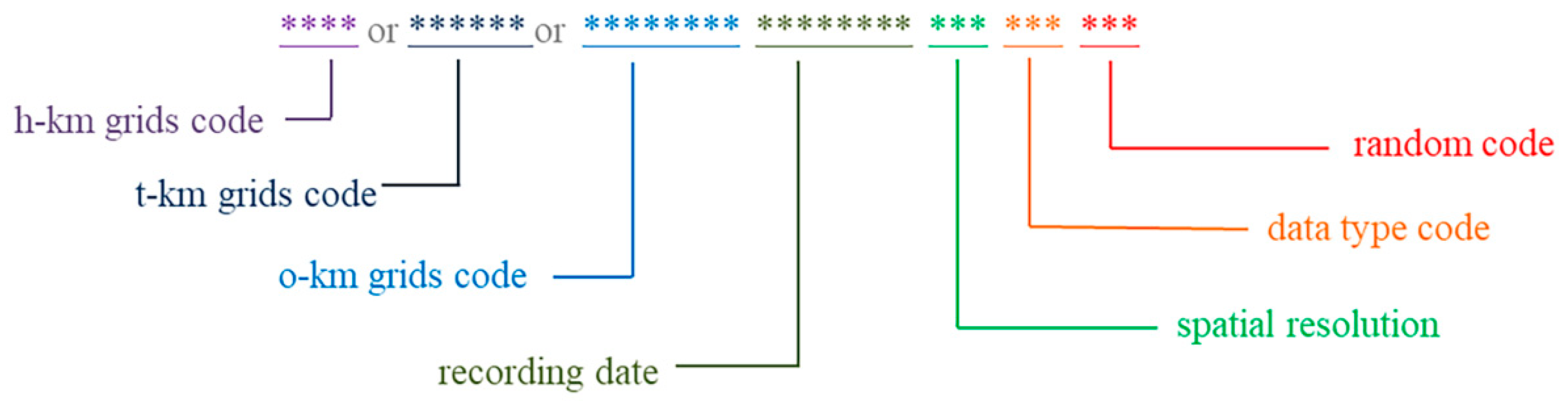
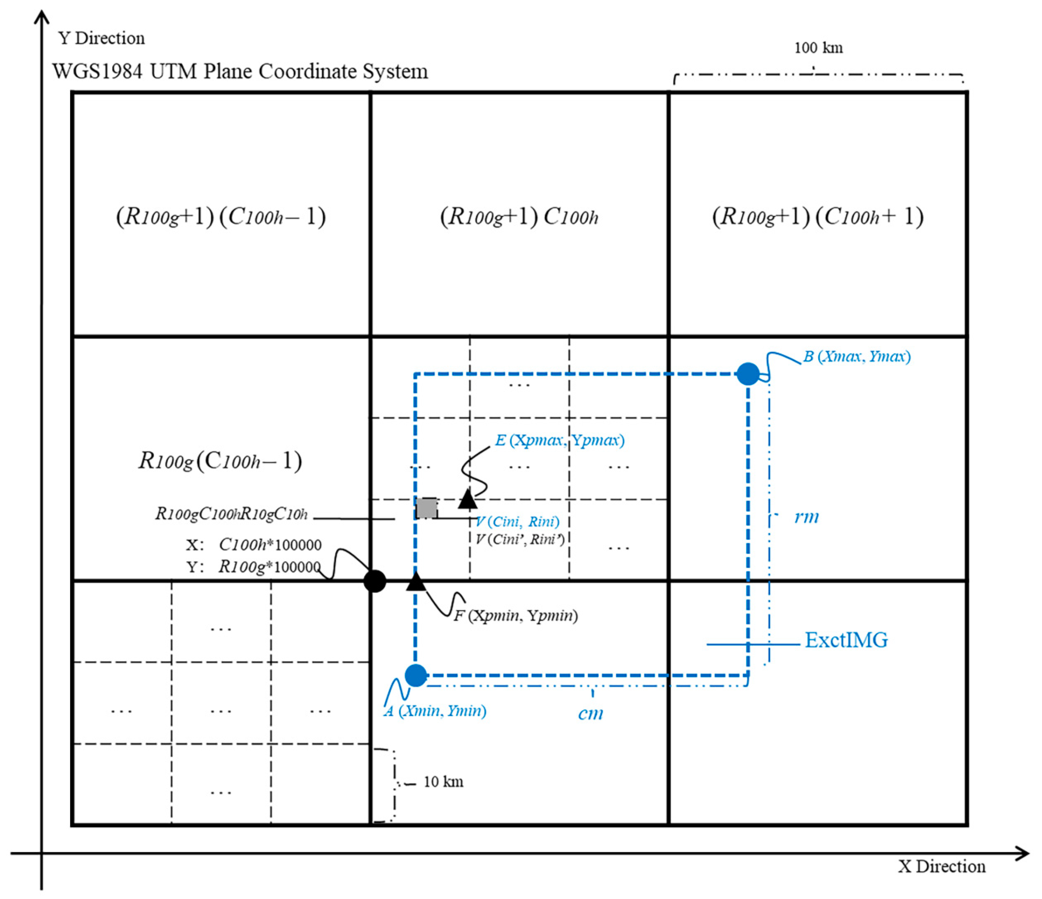
2.3. Mutil-Grid Partition and Coding Strategy

Considering grid universality, the design of the RDCRMG referenced China’s national geographic grid standard. Three levels of square grids were generated with different grid sizes and strict nested relationships (one-hundred-km grid (h-km grid), ten-km grid (t-km grid) and one-km grid (o-km grid)), as Figure 1 shows. Each level of grids has been used as a basic partition and organizational unit of raster files with specific spatial resolutions, as

Table 1. Organization Unit of Different Raster Data Type.

No.	Data Type	Modified Spatial Resolution *	Grid Level	Matrix Size	Data Type Code
1	GDEM	32	h-km grid	3125 × 3125	011
2	GlobalLand30	32	h-km grid	3125 × 3125	021
3	GF-1 WFV Multispectral	16	t-km grid	625 × 625	031
4	Sentinel 2A	10	t-km grid	1000 × 1000	041
5	GF-1 PMS Multispectral	8	t-km grid	1250 × 1250	032
6	RapidEye	5	t-km grid	2000 × 2000	051
7	GF-2 PMS Multispectral	4	t-km grid	2500 × 2500	034
8	GF-1 PMS Panchromatic	2	o-km grid	500 × 500	033
9	GF-2 PMS Panchromatic	1	o-km grid	1000 × 1000	035
10	World View-1	0.5	o-km grid	2000 × 2000	061

* Modified spatial resolution unit: meter.

shows. H-km grids are used for organizing 20–50 m raster files, including GDEM, GlobalLand30, and Landsat TM. T-km grids are used for organizing four–16 m raster files with different matrix sizes; o-km grids are used for organizing 2-m, 1-m and 0.5-m raster files with corresponding matrix sizes of 500 × 500, 1000 × 1000, and 2000 × 2000, respectively. Grids in the same level have been generated line by line with uniform size, shape and orientation, and they have strict nested relationships with their upper level grid (if it exists). Each partitioned raster file block only belongs to one grid with an identical spatial boundary, and it does not have a spatial superposition relationship with file blocks in adjacent grids. Furthermore, since the RDCRMG-based applications have higher requirements on raster files extraction efficiency than file aggregation and scale conversion efficiency, the row-column structure is more applicable for grid partitions than the quad-tree structure. It has the advantages of lower query algorithm complexity and higher organization pattern consistency.

In terms of grid coding, h-km grids are coded with four digits. The first two digits and the last two digits respectively represent the third to fourth digits of the y-coordinate and x-coordinate of the grid’s southwest vertex (unit: km). As Figure 1a shows, the y-coordinate and x-coordinate of the h-km grid in the southwest vertex (M) are 5100 (km) and 500 (km), respectively, and the grid code is 5105. T-km grids are coded by appending two digits to code of the h-km grid which it belongs. These two additional digits respectively represent the numerical values of the y-coordinate and x-coordinate in the ten digit’s place (unit: km). As Figure 1b shows, the t-km grid’s southwest vertex (N) coordinate is 5130 (km) and 580 (km), and its corresponding code is 510538. Similarly, the code of the o-km grids consist of eight digits. The first six digits are the same as the code of the t-km grid to which it belongs, and the last two digits respectively represent the numerical values of the y-coordinate and x-coordinate in the single digit’s place (unit: km). As Figure 1d shows, the o-km grid’s southwest vertex (K) coordinate is 5132 (km) and 585 (km), and its corresponding code is 51053825. By using this strategy, h-km grids, t-km grids and o-km grids are coded with high consistency. The nested relationships of grids in different levels can be expressed in a simple form. Therefore, corresponding grid codes of spatial query ranges can be figured out through simple linear formulas, and the mathematical relationship between the pixel row-column number and the planar coordinates can be easily established. As Figure 1c shows, the GF-1 WFV 16-m raster file block has been organized by the t-km grid 510538. For any internal pixel m (C_m, R_m), its central point coordinate X_m = 580,000 + pix × (C_m + 0.5), Y_m = 5140,000 – pix × (R_m + 0.5) pix is its spatial resolution.

In actual applications, grid codes are not stored in relational data tables with their corresponding raster metadata. They are used as the directory name and file name to generate logical storage paths of raster file blocks based on the “no metadata” mode. Figure 2 presents the structure of the grid code-based raster file storage path. Root directories are named after the spatial coordinate system WKID (Spatial Reference Systems Well-known ID) and correspond to different UTM projection strips. On that basis, the lower level node directories have been created layer by layer and named after the h-km grid code, the t-km grid code and the o-km grid code for the storage of raster files with different spatial resolutions. Then, subdirectories have been created in the node directory of each layer and named after the recording date (year). Finally, the raster file blocks have been stored in the corresponding subdirectory as leaf nodes with specific name codes. As Figure 3 shows, the name code of the leaf node consists of five parts: the grid code, the recording date, the spatial resolution, the three digit data type number and the three digit random code. The grid code is in accordance with the RDCRMG code. The recording date marks come in eight digits: four digits for the year, two digits for the month and two digits for the day. Spatial resolution marks come in three digits. The data type number is predetermined in the data table (as Table 1 lists), and random code is used to avoid overriding files of the same name in the form of letters or figures. For each part, “0” should be added in the front if the actual value is insufficient for the designated digits. For example, as Figure 1c shows, the GF-1 WFV 16-m raster file block covers the t-km grid 510538. And it was recorded on 13 August 2014. Then its name code can be expressed as 51053820140813016031BKF. In the other example, the storage path of the GF-1 16-m RS file block that covers the t-km grid 510543 and was recorded on 5 July 2015 can be rapidly generated as …\32651\5105\43\2015\51054320150705016031***.dat. On that basis, raster file blocks can be rapidly extracted and merged in parallel according to the required spatial-temporal query conditions.

Through our RDCRMG-based raster file partition and coding strategy, raster file blocks have been discretely stored in several data nodes to increase data parallel transmission efficiency. Considering the spatial correlation of raster data, file blocks relevant to adjacent grids will be stored in the same data node through which network loads can be lessened as far as possible in the data calculation process. Furthermore, by using the “no metadata” mode, relevant grid codes and file block storage paths can be directly calculated in the spatial query process. Therefore, the time consumption on metadata retrieval can be reduced, and potential failures and performance bottlenecks of metadata nodes can be avoided.

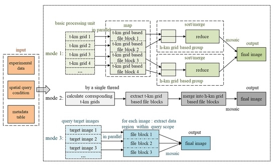
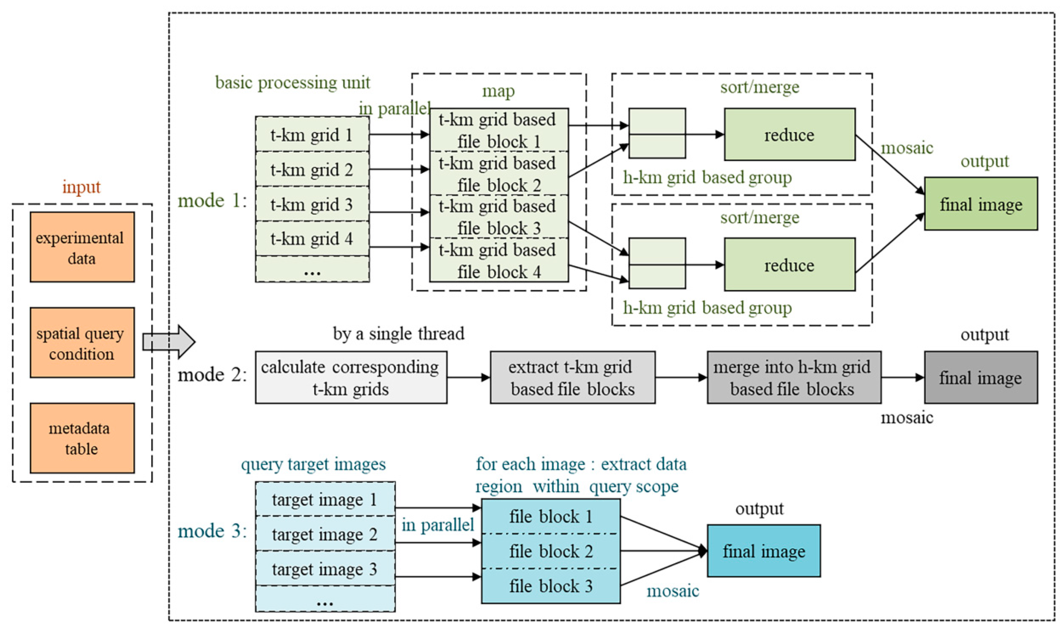
2.4. Mutil-Grid Based Data Retrieval Strategy

The RDCGMG-based raster data retrieval workflow has been listed below. The pre-conditions are the known query scope, observation period and target data type.

Step 1 analyzes the spatial query range, extracts the vertex coordinates (L_min, B_min, L_max, B_max) of its least surrounding rectangle (LSR) and reads its geospatial coordinate reference system information. The analytical or numerical method should be executed to transform the coordinate reference system to the WGS 1984 geographic coordinate system if necessary.

Step 2 distinguishes whether the LSR crosses multiple projection zones, as Equation (1) shows. “⌊ ⌋” is the round-down symbol. $\Delta$ is the tolerable error and is set as 0.0001°. If not, then we calculate the corresponding planar coordinates of the LSR (the plane coordinate system is in accordance with that of projection zone) and use it as the query task unit. Otherwise, the LSR will be subdivided into several mutually independent sub-rectangles by projection zone boundaries. Each sub-rectangle corresponds with one projection zone and works as a query task unit.

$$\left(\lfloor L_{max}/6\rfloor \times 6-\Delta >L_{min}\right)?\mathrm{cross}:\mathrm{not}\mathrm{cross}$$

(1)

Step 3 splits the query task unit range into several non-overlapping sub-ranges based on the custom rule. Then, the raster file $\mathrm{ExctIMG}\left[\mathrm{cm},\mathrm{rm},\mathrm{n}\right]$ is constructed for each sub-range. Therefore, cm and rm respectively express the column count and row count of $\mathrm{ExctIMG}$, and n expresses the waveband count. On that basis, the process of writing data to $\mathrm{ExctIMG}$ can be executed in parallel.

Step 4 calculates the corresponding grid codes and file block storage paths of each $\mathrm{ExctIMG}$. By taking the query t-km grid-based GF-1 RS data that was observed on 1 July 2015 as an example, the vertex coordinates of $\mathrm{ExctIMG}$ are A (X_min, Y_min) and B (X_max, Y_max), as Figure 4 shows. The relevant t-km grid codes R_100gC_100hR_10gC_10h of $\mathrm{ExctIMG}$ can be calculated by a linear polynomial, as Equation (2) lists. Therefore, the directory path of the relevant file blocks can be generated as “…\WKID\R_100gC_100h\R_10gC_10h\2015\”.

$$R_{100g} =\lfloor \left(Y_{min}/10,000+g\right)/10\rfloor , C_{100h} =\lfloor \left(X_{min}/10,000+\mathrm{h}\right)/10\rfloor$$

$$R_{10g} =\left(\lfloor Y_{min}/10,000\rfloor -\lfloor Y_{min}/100,000\rfloor \times 10+g\right)\%10$$

$$C_{10\mathrm{h}} =\left(\lfloor X_{min}/10,000\rfloor -\lfloor X_{min}/100,000\rfloor \times 10+\mathrm{h}\right)\%10$$

$$\mathrm{thereinto},g=\left\{0,1\dots ,\lfloor Y_{max}/10,000\rfloor -\lfloor Y_{min}/10,000\rfloor \right\}$$

$$\mathrm{h}=\left\{0,1\dots ,\lfloor X_{max}/10,000\rfloor -\lfloor X_{min}/10,000\rfloor \right\}$$

(2)

Step 5 reads each pixel value from the relevant file blocks and writes it into the corresponding position for each $\mathrm{ExctIMG}$. Figure 4 presents the RDCRMG-based raster data extraction method in the t-km grid level. For any t-km grid R_100gC_100hR_10gC_10h that intersects with $\mathrm{ExctIMG}$, its vertex coordinates E (X_pmax, Y_pmax) and F (X_pmin, Y_pmin) can be expressed as X_pmin = max (X_min, (C_100h × 10 + C_10h) × 10,000), Y_pmin = max (Y_min, (R_100g × 10 + R_10g) × 10,000), X_pmax = min (X_max, (C_100h × 10 + C_10h + 1) × 10,000), and Y_pmax = min (Y_max, (R_100g × 10 + R_10g + 1) × 10,000). Max() is the maximum symbol, and min() is the minimum symbol. Then, the mathematical relationship between the file blocks and $\mathrm{ExctIMG}$ will be constructed, as Equation (3) lists. GridIMG is the relevant raster matrix of grid R_100gC_100hR_10gC_10h. $\partial x$ and $\partial y$ represent the spatial resolution of the target raster data in X direction and Y direction. For the initial pixel V of the overlapping area between $ExctIMG$ and GridIMG, $C_{ini}$ and $R_{ini}$ corresponds with column No. and row No. of V in $ExctIMG$, while $C_{ini}’$ and $R_{ini}’$ is that in GridIMG. Furthermore, the raster calculation among different wavelength images can be integrated in $ExctIMG’\mathrm{s}$ generation process to reduce the data volume and thereby increase transmission efficiency.

$$ExctIMG\left[C_{ini}+k, R_{ini}+w\right]=GridIMG\left[C_{ini}\prime +k, R_{ini}\prime +w\right]$$

$$C_{ini}=\lfloor \frac{X_{pmin}-X_{min}}{\partial x}\rfloor ,\hspace{1em}\hspace{1em}{R}_{ini}=\lfloor \frac{Y_{max}-Y_{pmax}}{\partial y}\rfloor$$

$$C_{ini}’=\lfloor \frac{X_{pmin}-\left(C_{100h}\times 10+C_{10h}\right)\ast 10,000}{\partial x}\rfloor , R_{ini}’=\lfloor \frac{\left(R_{100h}\times 10+R_{10h}+1\right)\ast 10,000-Y_{pmax}}{\partial y}\rfloor$$

$$k=\left\{0, 1,\dots ,\hspace{1em}\hspace{1em}\lfloor \frac{X_{pmax}-X_{pmin}}{\partial x}\rfloor \right\},\hspace{1em}\hspace{1em}w=\left\{0,1,\dots ,\hspace{1em}\hspace{1em}\lfloor \frac{Y_{pmax}-Y_{pmin}}{\partial y}\rfloor \right\}$$

(3)

Step 6 merges the $ExctIMG$ that was derived from the same query task unit into one result image. Each result image corresponds with a UTM projection zone.

Step 7 exports the final results and finishes the raster data retrieval task. The final result can be several independent result images organized by different planar coordinate systems or one merged image organized by a user-defined spatial coordinate system.

The characteristics of our RDCGMG-based raster data retrieval strategy are listed as follows:

• It uses the LSR of the spatial query range for data retrieval and transforming the spatial geometric relationship analysis to linear grid codes calculations and file blocks mosaics. While data redundancy may be increased, the computation complexity can be dramatically reduced.
• The data retrieval task can be easily assigned to several grid groups and executed in parallel. For each grid group, the relevant file blocks are merged similarly to jigsaw puzzles.
• The final result can be several independent images, which make it more efficient for image calculation and expression, especially when the query scope is large.

3. RDCRMG-Based Raster Data Extraction Results

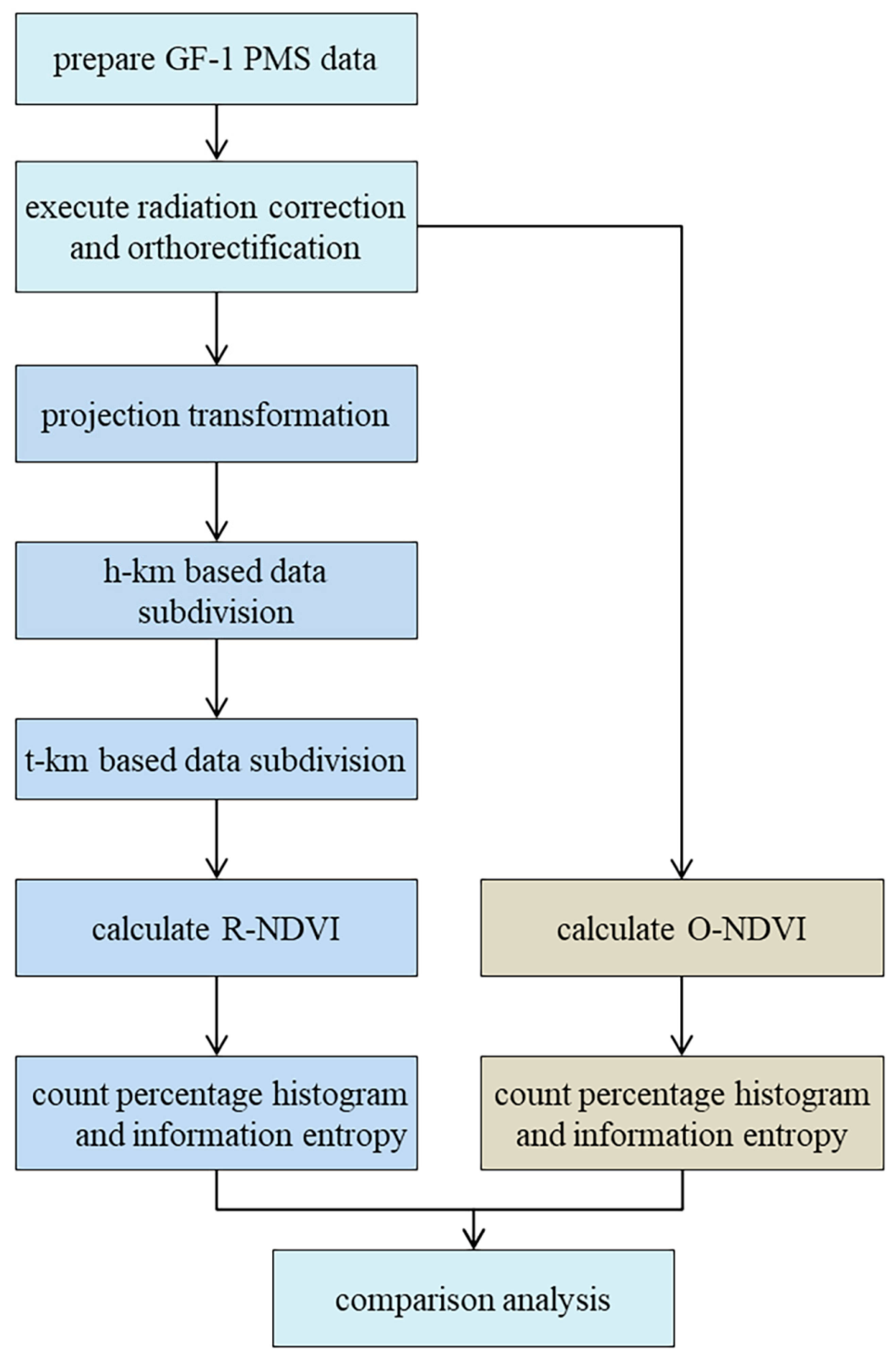
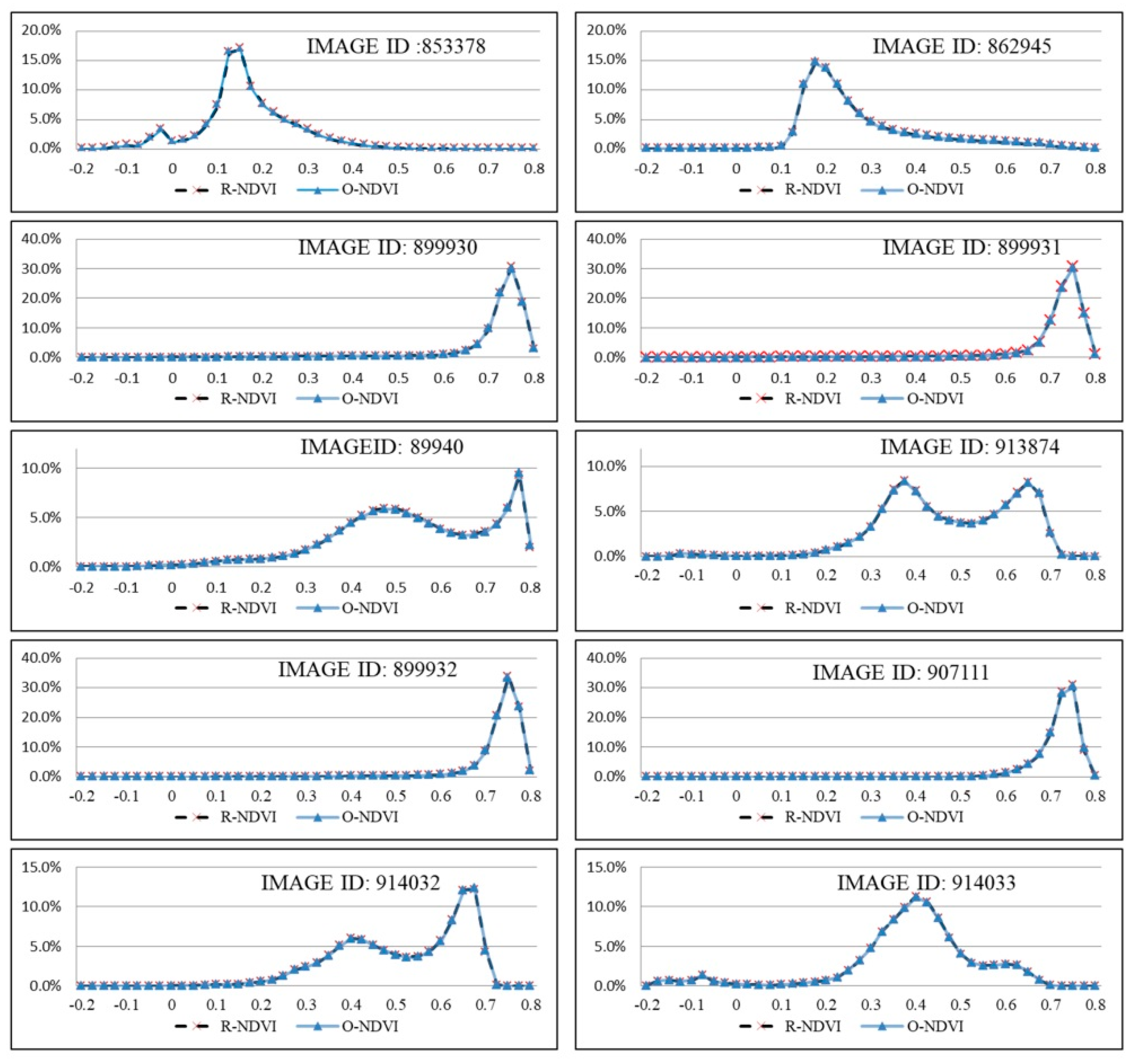
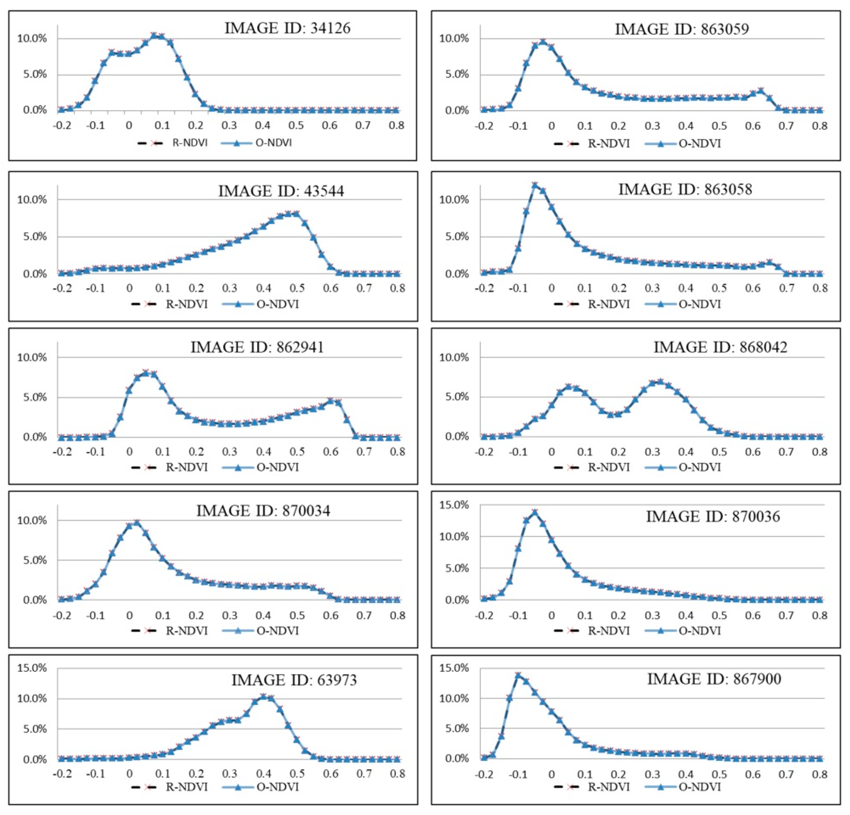
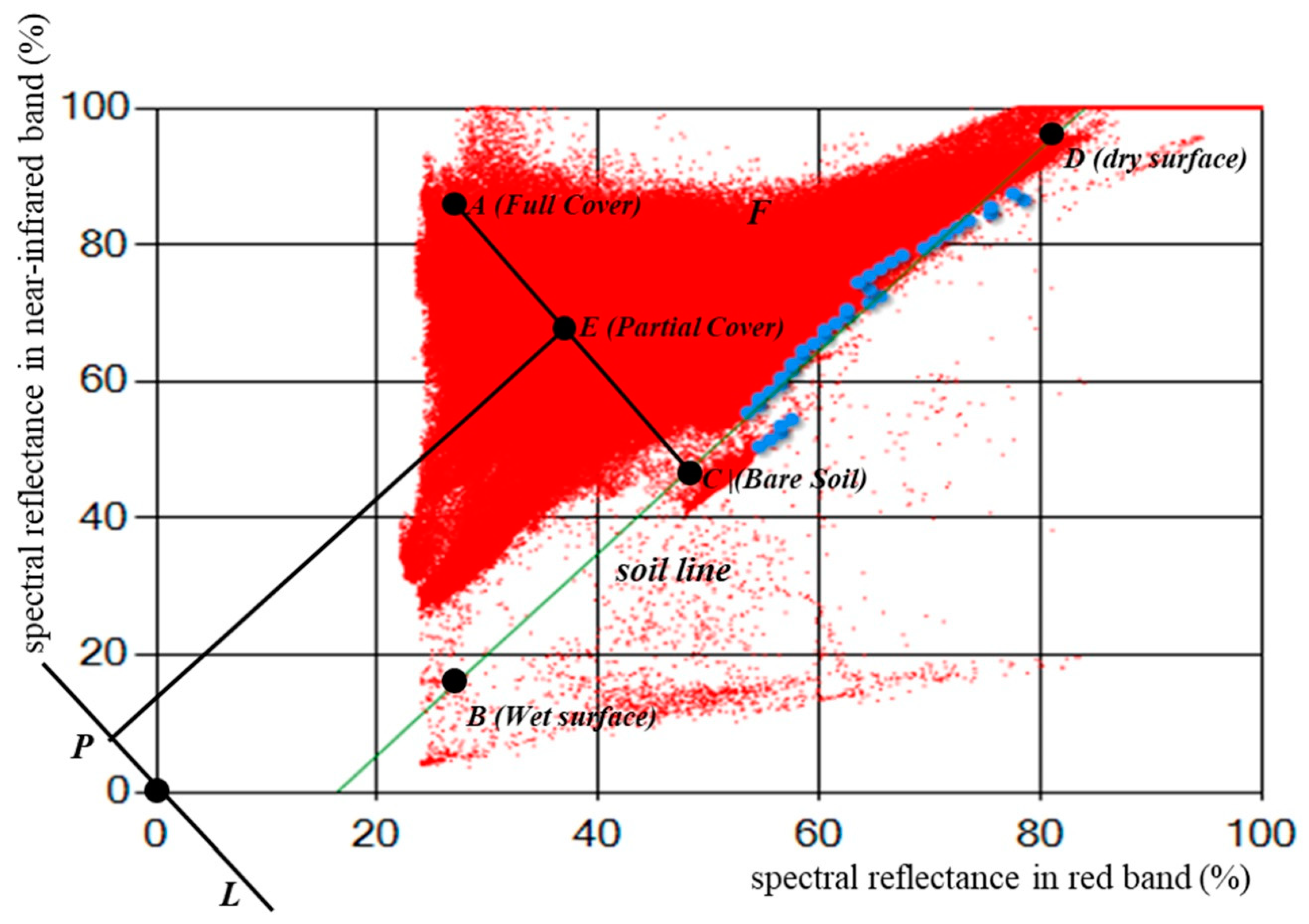
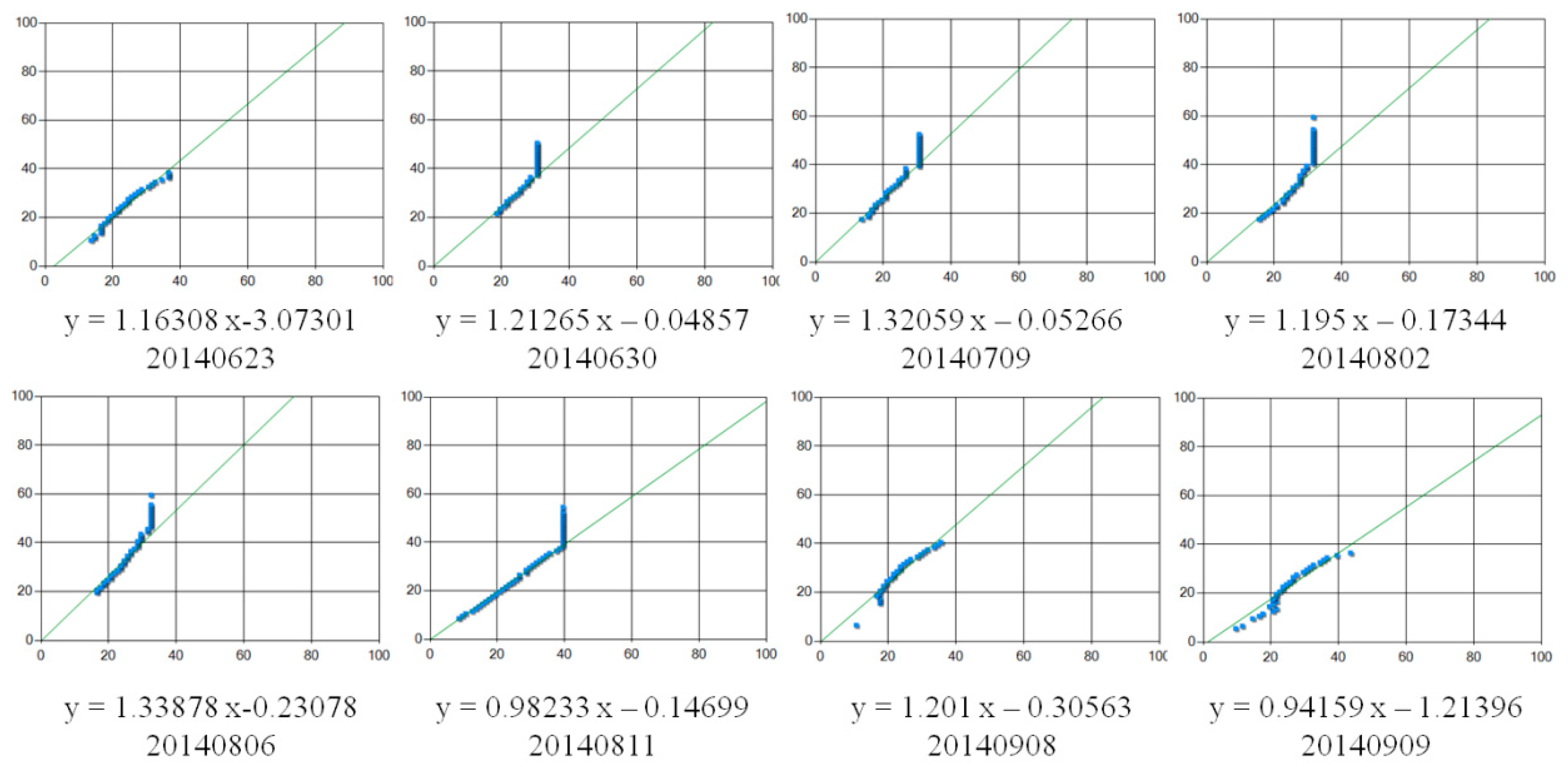
3.1. Pixel Spectral Reflectance Variation Detection

Spectral reflectance is a crucial factor for vegetation dryness remote sensing monitoring. To transform multi-source RS data into a consistent organizational and storage rule, data manipulations (including clip, resample, coordinate transformation and cleaning) should be executed. These manipulations may distort the pixel spectral reflectance information and thereby affect the monitoring accuracy. However, even if the RDCRMG is not used, the spectral reflectance distortion is still unavoidable in data pre-processing or fusion.

In this paper, comparison experiments of pixel spectral reflectance have been performed to raster data organized in both the RDCRMG mode and the traditional framing mode; 20 GF-1 PMS images observed from June to August (when plants thrive in the northern hemisphere) have been selected as the experimental data. These images can be uniformly divided into two groups, A and B. Images in group A belong to one single projection zone and images in group B cross more than one projection zone. For each image, radiation correction and orthorectification have been executed.

Figure 5 presents the spectral reflectance variation detection experiments’ workflow. Each image has been processed using two modes. For one mode, images have been split into several file blocks base on the RDCRMG t-km grids and reconstructed according to their original boundary. Then, the normalized differential vegetation index (NDVI,) has been calculated (R-NDVI for short), where $\mathrm{NIR}$ and $\mathrm{R}$ represent the spectral reflectance in near-infrared band and red band, respectively. For the other mode, NDVI has been directly calculated (O-NDVI for short). On that basis, the percentage histogram and information entropy $\mathrm{H}$ of R-NDVI and O-NDVI have been calculated as indicators for comparison. Statistics of the percentage histogram have been executed by dividing the value domain of NDVI [−1, 1] into 80 ranges (the interval is 0.025). Equation (4) presents the polynomial for the information entropy (H). $P_i$ (i = 1, 2,…, 400) is the percentage of NDVI, which is counted by dividing the value domain into 400 ranges (the interval is 0.005).

$$H=-{\displaystyle \sum }_{i=1}^n{P}_i{log}_2{P}_i$$

(4)

Figure 6 and Figure 7 represent the differences of the percentage histograms between R-NDVI and O-NDVI for group A and group B, respectively. The relevant similar distance $D_{ndvi}$ has been listed in

Table 2. Similar Distance between R-NDVI and O-NDVI.

Group A				Group B
Image ID	${\mathit{D}}_{\mathit{n}\mathit{d}\mathit{v}\mathit{i}}$	Image ID	${\mathit{D}}_{\mathit{n}\mathit{d}\mathit{v}\mathit{i}}$	Image ID	${\mathit{D}}_{\mathit{n}\mathit{d}\mathit{v}\mathit{i}}$	Image ID	${\mathit{D}}_{\mathit{n}\mathit{d}\mathit{v}\mathit{i}}$
853378	0.0002761	899930	0.0008951	34126	0.0000965	863059	0.0000519
862945	0.0004677	899931	0.0004937	43544	0.0000243	867900	0.0000748
907111	0.0001211	899932	0.0009110	63973	0.0000770	868042	0.0000916
914032	0.0003259	899940	0.0004031	862941	0.0000967	870034	0.0000515
914033	0.0002150	913874	0.0004272	863058	0.0000266	870036	0.000317

. Equation (5) presents the polynomial for $D_{ndvi}$; $w_j$ and $k_j$ respectively represent the percentages of R-NDVI and O-NDVI in the range j (j = 1, 2,…, 80), and $\mathrm{n}$ is the range count. Experimental results show that the percentage histograms of R-NDVI and O-NDVI are basically the same. The $D_{ndvi}$ results in group A are less than 0.0009110, and the results in group B are even smaller (less than 0.0000965). The difference of information entropy between R-NDVI and O-NDVI is small, as

Table 3. Information Entropy of R-NDVI and O-NDVI in Group A and Group B.

Group A				Group B
Image ID	Observing Date	$\mathit{H}$ of O-NDVI	$\mathit{H}$ of R-NDVI	Image ID	Observing Date	$\mathit{H}$ of O-NDVI	$\mathit{H}$ of R-NDVI
853378	10 June 2015	6.2291147	6.2212885	34126	15 June 2015	6.1041904	6.1042737
862945	14 June 2015	6.3906426	6.3820948	43544	5 July 2013	6.8720507	6.8718363
907111	9 July 2015	4.8870048	4.8579931	63973	6 August 2013	6.4693812	6.4680682
914032	13 July 2015	6.5100051	6.5040877	862941	14 June 2015	6.9930203	6.9909612
914033	13 July 2015	6.6216194	6.6125231	863058	14 June 2015	6.8748594	6.8737988
899930	5 July 2015	5.2704958	5.2540650	863059	14 June 2015	7.0331230	7.0320470
899931	5 July 2015	5.2082725	5.1953808	867900	17 June 2015	6.3188119	6.3181604
899932	5 July 2015	4.9820212	4.9622307	868042	17 June 2015	6.8142379	6.8151115
899940	5 July 2015	6.9523657	6.9416525	870034	18 June 2015	6.8816083	6.8804745
913874	13 July 2015	6.6584797	6.6421337	870036	18 June 2015	6.4055547	6.4055478

shows. For results in group A, the $\mathrm{H}$ of R-NDVI is slightly smaller than that of O-NDVI, which indicates that most information is preserved and in accordance with the concept that information will not be “created” during data processing. For results in group B, the $\mathrm{H}$ of R-NDVI may slightly larger than that of O-NDVI. This difference is because in the RDCRMG-based image partitioning process, the value of pixels on the projection zone boundary will be tautologically stored in adjacent file blocks. However, this phenomenon is beneficial for data consistency, and no nonexistent information is created.

In conclusion, as our comparison experiments show, the distortion of pixel spectral reflectance information caused by the RDCRMG-based RS data reconstruction mode is slight. RDCRMG is appropriate for vegetation dryness monitoring-oriented RS data organization.

$$D_{ndvi}=\sqrt{\raisebox{1ex}{${{\displaystyle \sum }}_{j=1}^{80}{\left(w_j-k_j\right)}^2$}\!\left/ \!\raisebox{-1ex}{$n$}\right.}$$

(5)

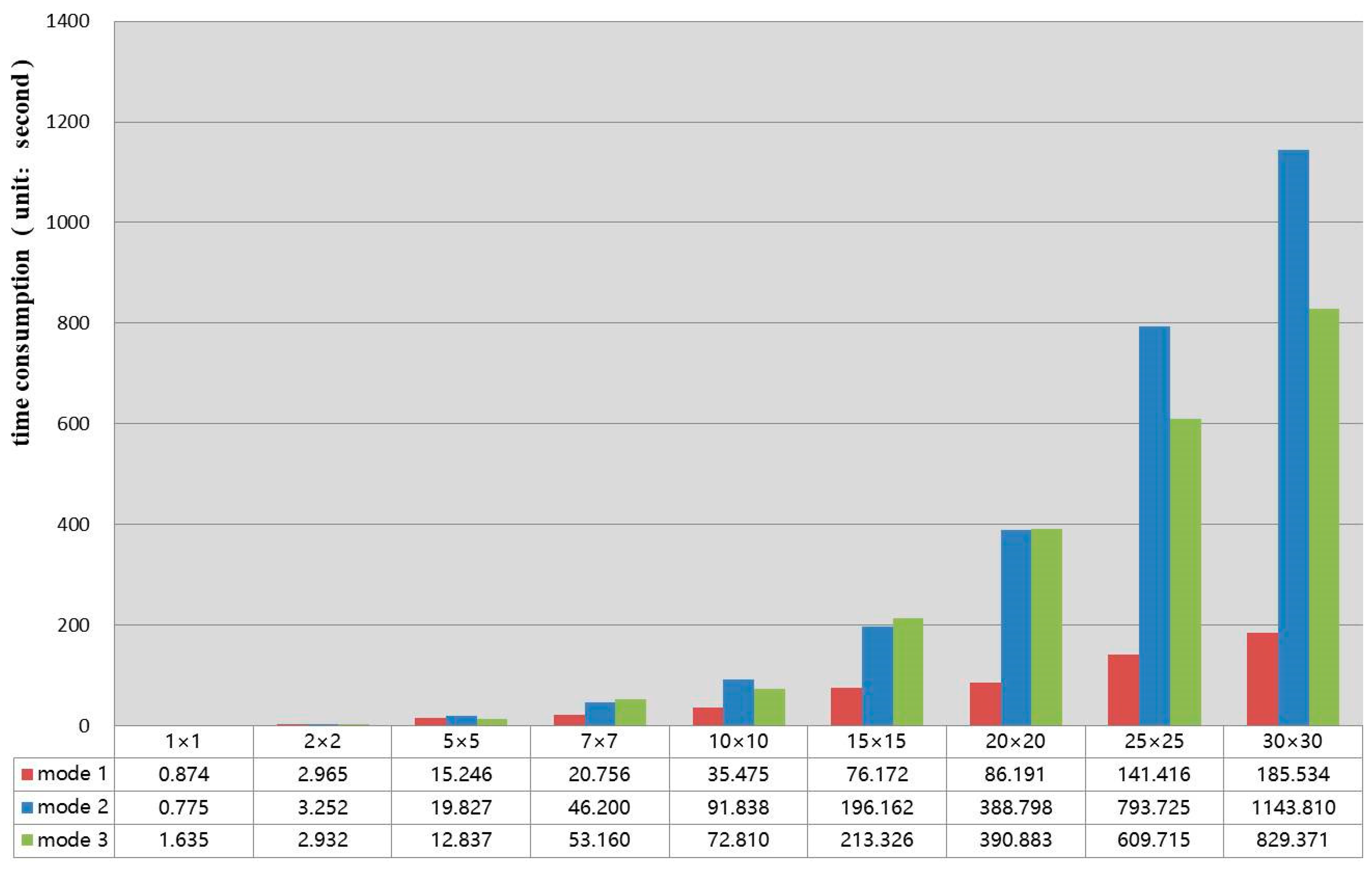
3.2. Data Extraction Efficiency Test

How much does the RDCRMG architecture promote the raster data extraction efficiency comparing with the traditional framing architecture? To answer this question, three modes have been used to execute data extraction tasks with different query scopes, as Figure 8 shows. The GF-1 PMS multispectral images have been used as experimental data.

For mode 1, the RDCRMG retrieval strategy has been realized by referencing the map-reduce mode. Through calculating corresponding t-km grid codes of the query scope, file blocks of each grid have been extracted in parallel. All file blocks were grouped based on the h-km grid and then merged in groups. At last, all group-based raster images are mosaicked into the final result. For mode 2, the above-mentioned t-km file blocks extraction and mosaicking process was executed in a single thread. For mode 3, the data extraction task was performed based on the traditional process. First, we calculate the target images while conforming to the spatial query condition. Second, we extract the data within the query scope for each image and export file blocks in parallel. Finally, we merge file blocks into the final result.

Figure 9 presents nine query scopes consisting of different numbers of t-km grids in the same projection zone, including one (1 × 1) grid, four (2 × 2) grids, 25 (5 × 5) grids, 49 (7 × 7) grids, 100 (10 × 10) grids, 225 (15 × 15) grids, 400 (20 × 20) grids, 625 (25 × 25) grids, and 900 (30 × 30) grids. For each group, the initial t-km grid in the northwest corner is coded 530390. The task-level parallelism-based computing cluster with four spatial analysis servers and one load balancing server has been deployed as the infrastructure for efficiency tests, as Figure 10 shows.

Figure 11 presents the data extraction time consumption of modes 1/2/3 with different sized query scopes. When the query scope is smaller than 50 × 50 km², the efficiency of mode 3 can be similar or even higher than mode 1. However, when the query scope increases, the efficiency of mode 1 gradually becomes higher than that of mode 3, and the trend becomes more significant. For extracting raster data that covers 300 × 300 km² (the corresponding pixel matrix is 37,500 × 37,500), the time consumption of mode 1 is nearly 22.37% greater than that of mode 3. In most cases, the efficiency of mode 2 is lower than that of mode 3, which illustrates that the efficiency gap between parallel computing and serial computing cannot be filled by the RDCRMG architecture.

4. RDCRMG-Based Vegetation Dryness Monitoring Application Results

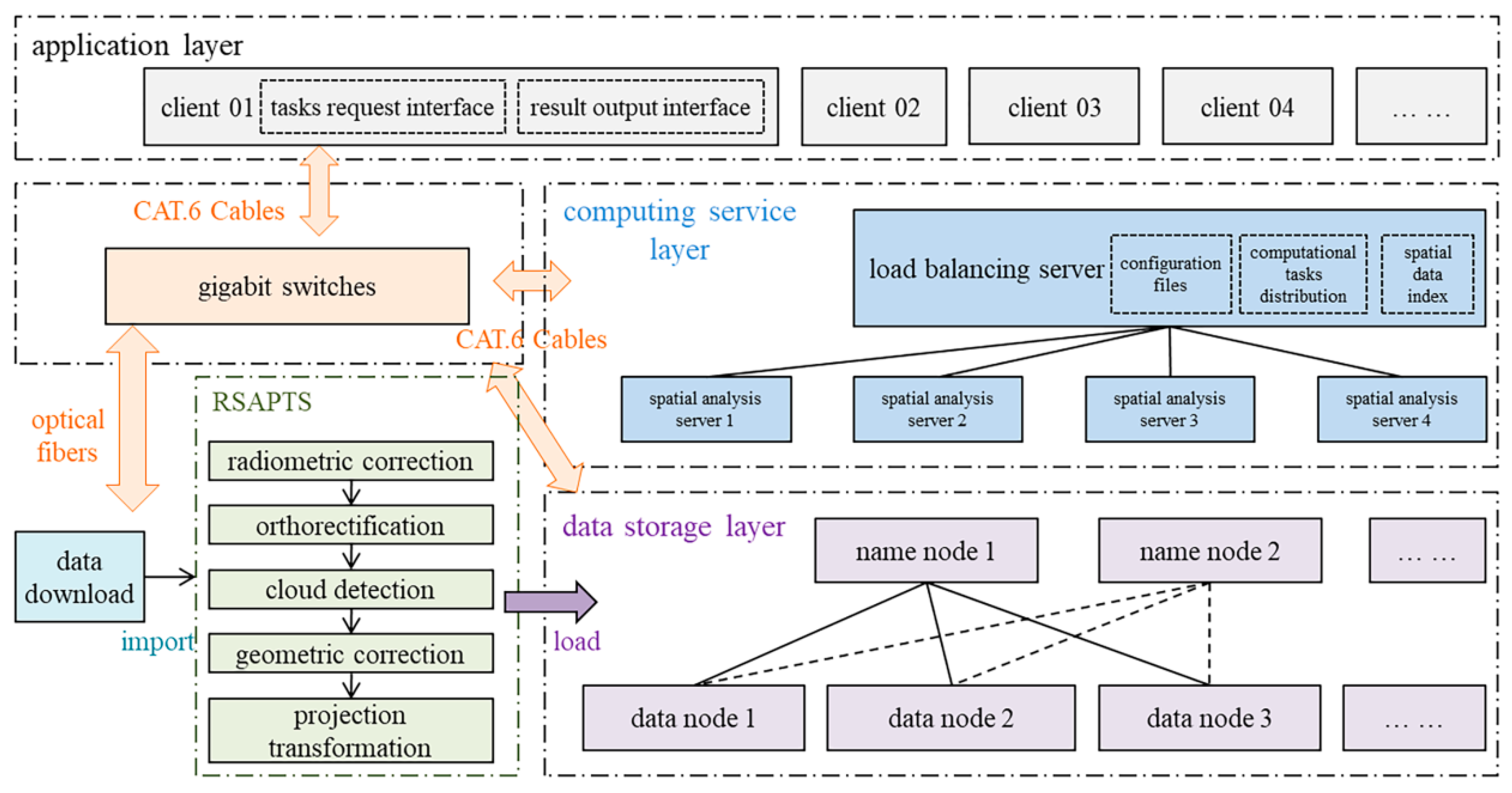
4.1. Experimental Environment

An RDCRMG-based vegetation dryness monitoring platform (VDMP) has been constructed to apply meso-scale and micro-scale, timely RS data inversion on vegetation dryness monitoring. Figure 11 presents the logical architecture of the VDMP infrastructure, including the data storage layer, the network transportation layer, the computing service layer and the application layer. In the data storage layer, the distributed metadata model-based file system was deployed on two name nodes and six data nodes. The RS data transfer is directly executed between computing service machines and data nodes, while name nodes are only used for metadata management and data addressing. The storage capacity is 200 TB, and both name nodes and data nodes can be horizontally extended. In the network transportation layer, gigabit switches and CAT.6 cables were used for data reading, analyzing and outputting; optical fibers were deployed for the RS data download. In the computing service layer, a computing cluster involving five computers was established for parallel data extraction and vegetation dryness inversion processing. The application layer integrates the task request interface and result output interface. Furthermore, an RS data automatic pretreatment system (RSAPTS) [37,38,39,40] was constructed to support near real time GF-1 RS data updating, including automatic radiometric correction, orthorectification [41], cloud detection, geometric correction [42] and projection transformation [43], up to 1 December 2017, 12612 GF-1 images were processed and loaded into the VDMP for vegetation dryness monitoring.

4.2. Automatic Vegetation Dryness Monitoring Strategy

The Perpendicular Drought Index (PDI) and Modified Perpendicular Drought Index (MPDI) [44,45] have been integrated in the VDMP as an RS inversion model on vegetation dryness monitoring. According to the PDI model, the scatter plot of the atmospheric corrected near-infrared band (NIR), red band (Red) reflectance spectrum demonstrated a typical triangle shape. F represents a point cloud of RS pixels in the NIR–Red feature space. Here, the AC line represents the change of surface vegetation from the full cover (A) and the partial cover (E) to bare soil (C) while BD refers soil moisture status for wet area (B), semi-arid surface to extremely dryness surface (D). It is not difficult to see from the Figure 12 that the dryness severity gradually rises from B to D, and reaches its climax at D. Here BD represents the soil line of the research area, which is established by using linear fitting to point cloud F, and its polynomial is $R_{nir}=M\times R_{red}+I$. $R_{red}$ and $R_{nir}$ are the spectral reflectance in the red band and near-infrared band, respectively; M refers to the slope of the soil line, I is the interception on the vertical axis. A line PL, which dissects the coordinate origin and is vertical to the soil line BD, can be delineated. Therefore, as to the normal function of a line, PL can be mathematically formulated as $R_{nir}=-\frac{1}{M}\times R_{red}$ from the soil line expression. The distance from any points in the NIR– Red reflectance space to the line L represents the dryness severity of the surface. The farther the distance, the stronger the dryness, and the less the soil moisture or vice versa. Taking a random point, a pixel E (Rred, Rnir) in the NIR–Red reflectance space, the vertical distance from E to line PL can be written as Equation (6).

$$\mathrm{PDI}=\frac{1}{\sqrt{M^2+1}}\left(R_{red}+M\times R_{nir}\right)$$

(6)

It is important to note that the PDI model is more applicable to vegetation dryness monitoring in barren or sparsely vegetated regions and is not comparable across regions with different land cover types. Therefore, the MPDI model has also been applied to vegetation dryness monitoring, as Equation (7) shows. $R_{red,v}$ and $R_{nir,v}$ are the respective maximum reflectivity of vegetation in the red band and near-infrared band, which are respectively set as 0.05 and 0.5; $f_v$ is the vegetation coverage. ${\mathrm{NDVI}}_{\mathrm{v}}$ and ${\mathrm{NDVI}}_{\mathrm{s}}$ respectively represent the NDVI of vegetation and bare soil and are correspondingly set as 0.65 and 0.2.

$$\mathrm{MPDI}=\frac{R_{red}+M\times R_{nir}-f_v\left(R_{red,v}+M\times R_{nir,v}\right)}{\left(1-f_v\right)\sqrt{M^2+1}}$$

$$f_v=={\left(\frac{\mathrm{NDVI}-{\mathrm{NDVI}}_{\mathrm{s}}}{{\mathrm{NDVI}}_{\mathrm{v}}-{\mathrm{NDVI}}_{\mathrm{s}}}\right)}^2$$

(7)

In actual applications of the MPDI-based or PDI-based vegetation dryness monitoring, the most important question is how to automatically calculate the soil line slope $\mathrm{M}$. In this paper, we reference the idea of tolerance in the variation function fitting process. The NIR–Red space has been divided into row-column-based homogeneous grids (grid interval is 0.01). Then, the pixel number of each grid was counted by iterating through each image relevant to the monitoring condition. On that basis, we select grids in the same row that share the same NIR reflectance interval as group S and count the percentage P1 of the group pixel number to the total pixel number. For each group, if P1 is less than the threshold value R1, the quantity of group S will be considered as too small to influence the soil line slope $\mathrm{MM}$. Otherwise, we iterate through each grid of group S from big to small along the Red reflectance intervals and count the percentage P2 of grid pixel number to the group pixel number. If P2 is less than the threshold value R², we count the next grid. Otherwise, we record the center point coordinate of this grid and break the grid traversal of the current group. R1 and R2 are respectively set as 0.2% and 0.05%. Lastly, the recorded center points-based least square method will be executed to calculate the soil line slope $\mathrm{M}$, through which the MPDI/PDI-based vegetation dryness situation can be automatically analyzed automatically.

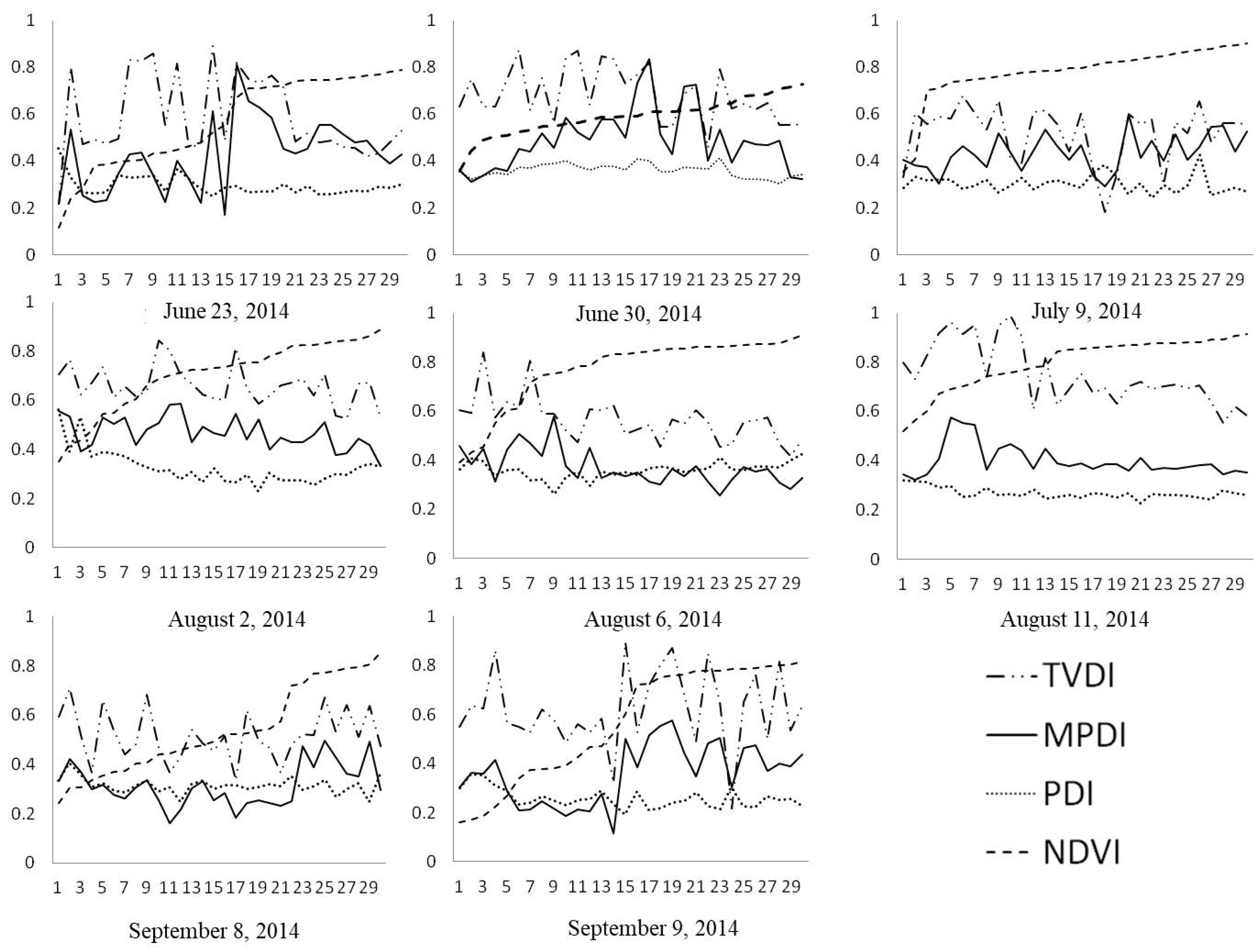
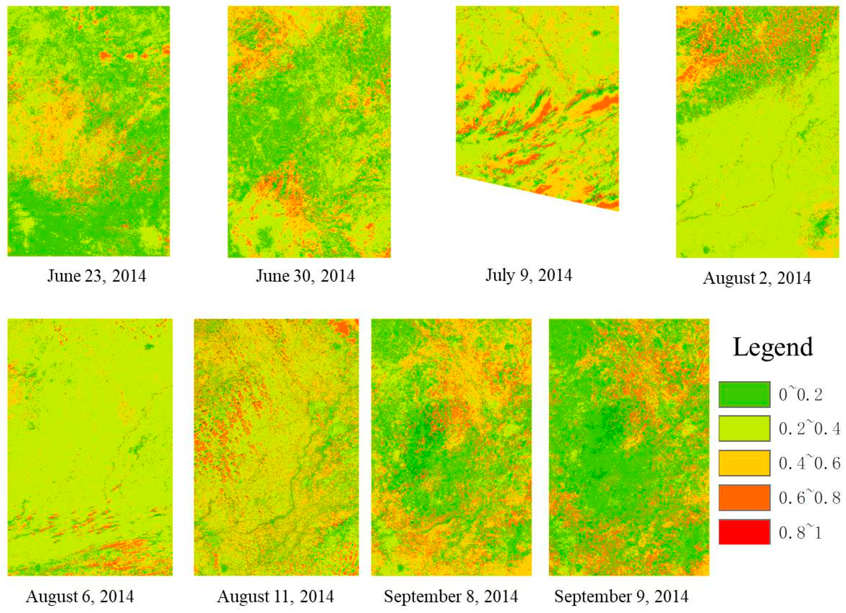
4.3. MPDI/PDI-Based Remote Sensing Monitoring Experiment

The MPDI/PDI-based vegetation dryness monitoring experiment has been constructed to test the practicability and reliability of the VDMP. We arranged our research area at the juncture of Fuxin city, Jinzhou city, Liaoyang city, Anshan city, and Shenyang city in the Liaoning province, which experienced a conspicuous drought disaster in 2014. The monitoring region covers east longitude of 122–23° and northern latitude of 41–42.5°, and the monitoring period is from 1 June 2014 to 30 September 2014. According to the abovementioned spatial-temporal query condition, 8 GF-1 images have been extracted by VDMP, as

Table 4. GF-1 & MODIS experimental data list.

Monitoring Date	GF-1 WFV	MODIS LST	MODIS NDVI
23 June 2014	L1A0000258243;L1A0000258242; L1A0000258241	MOD11A1.A2014174.h27v04.005.2014175145250.hdf	MOD13A2.A2014177.h27v04.006.2015288071235.hdf
30 June 2014	L1A0000263577; L1A0000263576	MOD11A1.A2014181.h27v04.005.2014182104028.hdf	MOD13A2.A2014193.h27v04.006.2015289002318.hdf
9 July 2014	L1A0000271504;	MOD11A1.A2014190.h27v04.005.2014191111312.hdf	MOD13A2.A2014209.h27v04.006.2015289031042.hdf
2 August 2014	L1A0000293356;L1A0000293355; L1A0000293368;L1A0000293367	MOD11A1.A2014214.h27v04.005.2014215101849.hdf	MOD13A2.A2014225.h27v04.006.2015289160437.hdf
6 August 2014	L1A0000296974;L1A0000296973; L1A0000296990	MOD11A1.A2014218.h27v04.005.2014219103329.hdf	MOD13A2.A2014225.h27v04.006.2015289160437.hdf
11 August 2014	L1A0000301288;L1A0000301287; L1A0000301299;L1A0000301298	MOD11A1.A2014223.h27v04.005.2014224102859.hdf	MOD13A2.A2014225.h27v04.006.2015289160437.hdf
8 September 2014	L1A0000336275;L1A0000336274; L1A0000336287;L1A0000336286	MOD11A1.A2014251.h27v04.005.2014252113357.hdf	MOD13A2.A2014225.h27v04.006.2015289160437.hdf
9 September 2014	L1A0000333819;L1A0000333818; L1A0000333817	MOD11A1.A2014252.h27v04.005.2014253150312.hdf	MOD13A2.A2014225.h27v04.006.2015289160437.hdf

shows. For each image, the soil line slope $\mathrm{M}$ was automatically calculated, as Figure 13 shows.

Furthermore, the MODIS Land Surface Temperature (LST) data (1 km, daily) and the MODIS NDVI data (1 km, compound of 16 days) were also extracted to calculate the Temperature Vegetation Dryness Index (TVDI) [46,47,48], as Table 4 shows. For each monitoring date, thirty uniformly distributed homonymous points were deployed in the MPDI data, the PDI data and the TVDI data to analyze the correlation of different models based on the linear polynomial fitting. As the experiment shows (

Table 5. Correlation analysis between MPDI/PDI and TVDI.

Monitoring Date	R2 of MPDI and TVDI	R2 of PDI and TVDI
23 June 2014	0.3632	0.0001
30 June 2014	0.3441	0.2755
9 July 2014	0.3816	0.083
2 August 2014	0.4509	0.0089
6 August 2014	0.4247	0.0653
11 August 2014	0.5561	0.0236
8 September 2014	0.4401	0.0587
9 September 2014	0.5163	0.087

), the MPDI is correlated with the TVDI. The correlation coefficients are within [0.4792, 0.5889], and the R-squared is within [0.3441, 0.5561]. The PDI shows a weak correlation with the TVDI. Figure 14 presents the MPDI, PDI, TVDI and NDVI values of different points for each monitoring date, and the horizontal coordinate is the sample point No. As shown in the figure, although the proportional relationship between the MPDI and the TVDI is not stable, the variation of the MPDI is basically consistent with the TVDI, and it can effectively reflect the changes in soil dryness. The variation of the PDI expresses weak similarity to TVDI and MPDI, especially in the region with high NDVI. As Figure 15 shows, the calculation result indicates that on 23 June 2014, the north-western area of the monitoring region experienced a severe dryness, while on 30 June 2014 the dryness area spread towards the southeast. Then, from 9 July 2014 to 11 August 2014, the dryness became more serious and persisted until 9 September 2014. This result is in accordance with the dryness monitoring information published by the China National Climate Centre. In conclusion, the RDCRMG-based VDMP is appropriate for meso-scale and micro-scale, timely vegetation dryness RS automatic monitoring; it demonstrates high-performance, high reliability and good extensibility.

5. Discussion

For most RS data center platforms, efficient RS data storage, retrieval and sharing have been realized by applying technologies such as NOSQL, Massive Distributed Storage, Parallel Computation, and Multistage Tile Maps. Multi grid systems are mainly used for spatial index without considering the difference of spatial range, format, data size and temporal-spatial resolutions of different types of RS datasets. In this paper, A Raster Dataset Clean & Reconstitution Multi-Grid (RDCRMG) architecture have been explained, by which different types of raster datasets have been partitioned, consistently organized and systematically applied. According to RDCRMG, three levels of square grids (100 km–10 km–1 km) with different grid sizes, strictly nested relationships and specific codes are used as consistent RS images partition units. This strategy shows several significant advantages. Firstly, adjacent blocks will be stored in the same data node. Data merging efficiency can be increased. Network load of data transmission can be lighten. Secondly, “no metadata model” can be integrated, by which target raster data can be speedily extracted without retrieving metadata records. Thirdly, the data retrieval task can be easily assigned to several grid groups and executed in parallel. Experiments have been done to test the raster data extraction efficiency of RDCRMG compared with the traditional framing architecture. According to our result, the RDCGMG-based data extraction in parallel circumstances (mode 1) has the advantages of high efficiency and excellent stability compared to that of the RDCGMG-based data extraction in serial circumstances (mode 2) and traditional data extraction (mode 3). When the query scope is smaller than 50 × 50 km², the efficiency of mode 3 is similar or even higher than mode 1. However, when the query scope increases, the efficiency of mode 1 gradually becomes higher than that of mode 3, and the trend becomes more significant. The time consumption of mode 1 is 185.534 s when the query scope covers 300 × 300 km² (the corresponding pixel matrix is 37,500 × 37,500, data volume is nearly 2.62 GB); mode 2 takes 1143.81 s, and mode 3 takes 829.371 s in the same case. Therefore, there will be no performance advantage for RDCRMG when the query scope is too small (e.g., smaller than 50 × 50 km² base on 10 km grids). And when the query scope is too big (e.g., bigger than 300 × 300 km² base on 10 km grids), the query task can be easily split into several sub-tasks and executed in parallel.

However, there are also some disadvantages for RDCRMG. Firstly, to transform multi-source RS data into a consistent organizational and storage rule, data manipulations (including clip, resample, coordinate transformation and cleaning) should be executed. These manipulations inevitably distort the pixel spectral reflectance information and thereby affect the monitoring accuracy. Comparison experiments of pixel spectral reflectance have been performed to GF-1 raster data organized in both the RDCRMG mode (R-NDVI) and the traditional framing mode (O-NDVI). As our comparison experiments showed, the percentage histograms of R-NDVI and O-NDVI are basically the same. The differences of information entropy between R-NDVI and O-NDVI are small. So we think that the distortion of pixel spectral reflectance information caused by the RDCRMG-based RS data reconstruction mode is slight. And RDCRMG is appropriate for vegetation dryness monitoring-oriented RS data organization. In our future works, we will continually study the influence of information distortion to different applications. Besides, the data manipulations process will be improved to reduce information loss. Secondly, we choose the WGS 84- based UTM 6-degree strip division projection coordinate system as the RDCRMG spatial reference on the basis of our design target and research scope. It does not mean that this spatial reference is better than polyhedron-based spatial reference or longitude/latitude -based spatial reference in any cases. RDCRMG is not applicable in global scale. For instance, RDCRMG cannot be used for organizing RS data that covers the two poles. In the future works, we will explore how to construct simple mathematical relationships between RDCRMG and Discrete Global Grid System so that these two types of multi grid systems can be integrated.

At last, an RDCRMG-based vegetation dryness monitoring platform (VDMP) has been constructed to apply meso-scale and micro-scale, timely RS data inversion on vegetation dryness monitoring. Furthermore, RS data automatic pretreatment workflow and modified automatic PDI / MPDI model have also been integrated in VDMP. Through actual applications, the RDCRMG architecture is proven to be appropriate for vegetation dryness RS automatic monitoring with better performance, more reliability and higher extensibility. However, only single RS dataset (e.g., GF-1, MODIS) is used in vegetation dryness monitoring without collaborative analysis of multi-source RS datasets. Our future works will focus on integrating different kinds of continuously updated RS data and meteorological observation data into the RDCRMG-based VDMP and studying multi-source RS datasets based on the collaborative analysis model for vegetation dryness monitoring. And since data preprocessing—data storage and management—data reading and calculation automatic workflow has been established in VDMP, more remote sensing inversion models and statistical modes (e.g., Random Forest, Deep Learning) will be integrated to provide more agricultural analysis services.

6. Conclusions

This paper reports on a Raster Dataset Clean & Reconstitution Multi-Grid (RDCRMG) architecture for remote sensing monitoring of vegetation dryness in which different types of raster datasets have been partitioned, consistently organized and systematically applied. Our RDCRMG-based change detection of the spectral reflectance information test and the data extraction efficiency comparative test shows that the RDCRMG is reliable for vegetation dryness monitoring with a slight reflectance information distortion (the resemble distance is less than 0.0009110) and consistent percentage histograms. Furthermore, the RDCGMG-based data extraction in parallel circumstances has the advantages of high efficiency and excellent stability compared to that of the RDCGMG-based data extraction in serial circumstances and traditional data extraction. The time consumption of mode 1 is 185.534 s when the query scope covers 300 × 300 km² (the corresponding pixel matrix is 37,500 × 37,500); mode 2 takes 1143.81 s, and mode 3 takes 829.371 s in the same case. At last, an RDCRMG-based vegetation dryness monitoring platform (VDMP) has been constructed to apply RS data inversion in vegetation dryness monitoring. Through actual applications, the RDCRMG architecture is proven to be appropriate for meso-scale and micro-scale, timely vegetation dryness RS automatic monitoring with better performance, more reliability and higher extensibility.

References

1. Wang, L.; Liu, J.; Yang, F.; Fu, C.; Teng, F.; Gao, J. Early recognition of winter wheat area based on GF-1 satellite. Trans. Chin. Soc. Agric. Eng. 2015, 31, 194–201. [Google Scholar]
2. Agrawal, S.; Joshi, P.K.; Shukla, Y.; Roy, P.S. SPOT VEGETATION multi temporal data for classifying vegetation in south central Asia. Curr. Sci. 2003, 85, 140–140. [Google Scholar]
3. Carleer, A.; Wolff, E. Exploitation of very high resolution satellite data for tree species identification. Photogramm. Eng. Remote Sens. 2004, 70, 135–140. [Google Scholar] [CrossRef]
4. Huang, J.; Tian, L.; Liang, S.; Ma, H.; Becker-Reshef, I.; Huang, Y.; Su, W.; Zhang, X.; Zhu, D.; Wu, W. Improving winter wheat yield estimation by assimilation of the leaf area index from Landsat TM and MODIS data into the WOFOST model. Agric. For. Meteorol. 2015, 204, 106–121. [Google Scholar] [CrossRef]
5. Huang, J.; Ma, H.; Su, W.; Zhang, X.; Huang, Y.; Fan, J.; Wu, W. Jointly Assimilating MODIS LAI and ET Products into the SWAP Model for Winter Wheat Yield Estimation. IEEE J. Sel. Top. Appl. Earth Obs. Remote Sens. 2015, 8, 4060–4071. [Google Scholar] [CrossRef]
6. Huang, J.; Wu, S.; Liu, X.; Ma, G.; Ma, H.; Wu, W.; Zou, J. Regional winter wheat yield forecasting based on assimilation of remote sensing data and crop growth model with Ensemble Kalman method. Trans. Chin. Soc. Agric. Eng. 2012, 28, 142–148. [Google Scholar]
7. Huang, J.; Ma, H.; Tian, L.; Wang, P.; Liu, J. Comparison of remote sensing yield estimation methods for winter wheat based on assimilating time-sequence LAI and ET. Trans. Chin. Soc. Agric. Eng. 2015, 31, 197–203. [Google Scholar]
8. GonzalezFlor, C.; Serrano, L.; Gorchs, G. Assessment of grape yield and composition using the reflectance based Water Index in Mediterranean rainfed vineyards. Remote Sens. Environ. 2012, 118, 249–258. [Google Scholar] [Green Version]
9. Main, R.; Cho, M.A.; Mathieu, R.; O’Kennedy, M.M.; Ramoelo, A.; Koch, S. An investigation into robust spectral indices for leaf chlorophyll estimation. ISPRS J. Photogramm. Remote Sens. 2011, 66, 751–761. [Google Scholar] [CrossRef]
10. Zarco-Tejada, P.J.; Miller, J.R.; Morales, A.; Berjón, A.; Agüera, J. Hyperspectral indices and model simulation for chlorophyll estimation in open-canopy tree crops. Remote Sens. Environ. 2004, 90, 463–476. [Google Scholar] [CrossRef]
11. Goodchild, M.F.; Guo, H.D.; Annoni, A.; Bian, L.; de Bie, K.; Campbell, F.; Craglia, M.; Ehlers, M.; van Genderen, J.; Jackson, D.; et al. Next-generation Digital Earth. Proc. Natl. Acad. Sci. USA. 2012, 109, 11088–11094. [Google Scholar] [CrossRef] [PubMed] [Green Version]
12. Cheng, C.X.; Song, X.M.; Zhou, C.H.; Zhu, Y. Generic cumulative annular-bucket histogram for spatial selectivity estimation of spatial database management system. Int. J. Geogr. Inf. Sci. 2013, 27, 339–362. [Google Scholar] [CrossRef]
13. Cheng, C.X.; Niu, F.Q.; Cai, J.; Zhu, Y.L. Extensions of GAP-tree and its implementation based on a non-topological data model. Int. J. Geogr. Inf. Sci. 2008, 22, 657–673. [Google Scholar] [CrossRef]
14. Cheng, C.X.; Lu, F.; Cai, J. A quantitative scale-setting approach for building multi-scale spatial databases. Comput. Geosci. 2009, 35, 204–2209. [Google Scholar] [CrossRef]
15. Fekete, G. Rendering and managing spherical data with sphere quadtrees. In Proceedings of 90 Proceedings of the 1st conference on Visualization, San Francisco, CA, USA, 23–26 October 1990. [Google Scholar]
16. Fekete, G.; Treinish, L.A. Sphere quadtrees: A new data structure to support the visualization of spherically distributed data. In Extracting Meaning from Complex Data: Processing, Display, Interaction, Proceedings of the Electronic Imaging: Advanced Devices and Systems, Santa Clara, CA, USA, 11–16 February 1990; SPIE: Bellingham, WA, USA, 1990; Volume 1259. [Google Scholar] [CrossRef]
17. Goodchild, M.F.; Yang, S.R. A hierarchical spatial data structure for global geographic information systems. CVGIP Graph. Models Image Process. 1992, 54, 31–44. [Google Scholar] [CrossRef] [Green Version]
18. Dutton, G. Universal Geospatial Data Exchange via Global Hierarchical Coordinates. In Proceedings of the International Conference on Discrete Global Grids, Santa Barbara, CA, USA, 26–28 March 2000. [Google Scholar]
19. Dutton, G. Encoding and handling geospatial data with hierarchical triangular meshes. In Proceedings of the 7th International Symposium on Spatial Data Handling, Delft, The Netherlands, 12–16 August 1996. [Google Scholar]
20. Zhou, M.Y.; Jian, J.C.; Gong, J.Y. A pole-oriented discrete global grid system: Quaternary quadrangle mesh. Comput. Geosci. 2013, 61, 133–143. [Google Scholar] [CrossRef]
21. Lukatela, H. Hipparchus. Data Structure: Points, Lines and Regions in Spherical Voronoi Grid. In Proceedings of the 9th International Symposium on Computer Assisted Cartography, Baltimore, MD, USA, 2–7 April 1989. [Google Scholar]
22. Wang, L.; Zhao, X.S.; Zhao, L.F. Multi-level QTM Based Algorithm for Generating Spherical Voronoi Diagram. J. Wuhan Univ. 2015, 40, 1111–1115, 1122. [Google Scholar]
23. Chen, S.P.; Zhou, C.H.; Chen, Q.X. New Generation of Grid Mapping. Sci. Surv. Mapp. 2004, 29, 1–4. [Google Scholar]
24. Li, D.R.; Xiao, Z.F.; Zhu, X.Y. Research on Grid Division and Encoding of Spatial Information Multi-Grids. Acta Geod. Cartograph. Sin. 2006, 1, 010. [Google Scholar]
25. Li, D.R.; Zhu, X.Y; Gong, J.Y. From Digital Map to Spatial Information Multi-grid—A Thought of Spatial Information Multi-grid Theory. J. Wuhan Univ. 2003, 6, 642–650. [Google Scholar]
26. Li, D.R. On the Typical Applications of Spatial Information Multi Grid. J. Wuhan Univ. 2004, 11, 945–950. [Google Scholar]
27. Li, D.R.; Shao, Z.F. Spatial Information Multi- grid and Its Functions. Geosp. Inf. 2005, 3, 1–3 and 5. [Google Scholar]
28. Bjørke, J.T.; Grytten, J.K.; Hæger, M.; Nilsen, S. A Global Grid Model based on Constant Area Quadrilaterals. In Proceedings of the 9th Scandinavian Research Conference on Geographical Information Science, Espoo, Finland, 4–6 June 2003. [Google Scholar]
29. Bjørke, J.T.; Nilsen, S. Examination of aconstant- area quadrilateral grid in representation of global digital elevation models. Int. J. Geogr. Inf. Sci. 2005, 8, 653–664. [Google Scholar]
30. Goodchild, M.F. Geographical Grid Models for Environ-mental Monitoring and Analysis across the Globe (panel session). In Proceedings of the GIS/LIS 94 Conference, Phoenix, AZ, USA, 25–27 October 1994. [Google Scholar]
31. Kimerling, A.J.; Sahr, K.; White, D.; Song, L. Comparing Geo-metrical Properties of Global Grids. Cartogr. Geogr. Inf. Sci. 1999, 26, 271–287. [Google Scholar] [CrossRef]
32. Cheng, C.Q.; Ren, F.H.; Pu, G.L. An Introduce to Spatial Information Subdivision Organization; Science Press: Beijing, China, 2012. [Google Scholar]
33. Lu, X.F.; Cheng, C.Q.; Gong, J.Y.; Guan, L. Review of data storage and management technologies for massive remote sensing data. Sci. China-Technol. Sci. 2011, 54, 3220–3232. [Google Scholar] [CrossRef]
34. Song, S.H. Global Remote Sensing Data Subdivision Organization Based on GeoSOT. Acta Geod. Cartogr. Sin. 2014, 43, 869–876. [Google Scholar]
35. Cheng, C.Q. The Global Subdivision Grid Based on Extended Mapping Division and Its Address Coding. Acta Geod. Cartogr. Sin. 2010, 39, 295–302. [Google Scholar]
36. Lewis, A.; Oliver, S.; Lymburner, L.; Evans, B.; Wyborn, L.; Mueller, N.; Raevksi, G.; Hooke, J.; Woodcock, R.; Sixsmith, J.; et al. The Australian Geoscience Data Cube—Foundations and lessons learned. Remote Sens. Environ. 2017, 202, 276–292. [Google Scholar] [CrossRef]
37. Ye, S. Research on application of Remote Sensing Tupu—take monitoring of meteorological disaster for example. Acta Geod. Cartogr. Sin. 2018, 47, 892–892. [Google Scholar]
38. Yao, X.C.; Mokbel, M.F.; Alarabi, L.; Eldawy, A.; Yang, J.; Yun, W.; Li, L.; Ye, S.; Zhu, D. Spatial coding-based approach for partitioning big spatial data in Hadoop. Comput. Geosci. 2017, 106, 60–67. [Google Scholar] [CrossRef]
39. Yao, X.; Mokbel, M.; Ye, S.; Li, G.; Alarabi, L.; Eldawy, A.; Zhao, Z.; Zhao, L.; Zhu, D. LandQv2: A MapReduce-Based System for Processing Arable Land Quality Big Data. ISPRS Int. J. Geoinf. 2018, 7, 271. [Google Scholar] [CrossRef]
40. Yao, X.C.; Yang, J.Y.; Li, L.; Ye, S.J.; Yun, W.J.; Zhu, D.H. Parallel Algorithm for Partitioning Massive Spatial Vector Data in Cloud Environment. J. Wuhan Univ. 2017, 10, 1–6. [Google Scholar]
41. Ye, S.; Zhang, C.; Wang, Y.; Liu, D.; Du, Z.; Zhu, D. Design and implementation of automatic orthorectification system based on GF-1 big data. Trans. Chin. Soc. Agric. Eng. 2017, 33, 266–273. [Google Scholar]
42. Yuan, W.; Sijing, Y.; Yueli, Y. Contrast of automatic geometric registration algorithms for GF-1 remote sensing image. Trans. Chin. Soc. Agric. Mach. 2015, 46, 260–266. [Google Scholar]
43. Ye, S.; Yan, T.; Yue, Y.; Lin, W.; Li, L.; Yao, X.; Mu, Q.; Li, Y.; Zhu, D. Developing a reversible rapid coordinate transformation model for the cylindrical projection. Comput. Geosci. 2016, 89, 44–56. [Google Scholar] [CrossRef]
44. Ghulam, A.; Qin, Q.; Zhan, Z. Designing of the perpendicular drought index. Environ. Geol. 2007, 52, 1045–1052. [Google Scholar] [CrossRef]
45. Ghulam, A.; Qin, Q.; Teyip, T.; Li, Z. Modified perpendicular drought index (MPDI): A real-time drought monitoring method. ISPRS J. Photogramm. Remote Sens. 2007, 62, 150–164. [Google Scholar] [CrossRef]
46. Bayarjargal, Y.; Karnieli, A.; Bayasgalan, M.; Khudulmur, S.; Gandush, C.; Tucker, C.J. A comparative study of NOAA–AVHRR derived drought indices using change vector analysis. Remote Sens. Environ. 2006, 105, 9–22. [Google Scholar] [CrossRef]
47. Ji, L.; Peters, A. Assessing vegetation response to drought in the northern Great Plains using vegetation and drought indices. Remote Sens. Environ. 2003, 87, 85–98. [Google Scholar] [CrossRef]
48. Martínez-Fernández, J.; González-Zamora, A.; Sánchez, N.; Gumuzzio, A.; Herrero-Jiménez, C.M. Satellite soil moisture for agricultural drought monitoring: Assessment of the SMOS derived Soil Water Deficit Index. Remote Sens. Environ. 2016, 177, 277–286. [Google Scholar] [CrossRef]
Figure 1. Raster Dataset Clean & Reconstitution Multi-Grid (RDCRMG) Grid Partition and Coding Strategy. (a) hundred km grids layer; (b) ten km grids layer; (c) single ten km grid case; and (d) km grids layer.
Remotesensing 10 01376 g001
Figure 2. RDCRMG based Raster File Blocks Storage Path.
Remotesensing 10 01376 g002
Figure 3. RDCRMG based Raster File Blocks Name Code Structure.
Remotesensing 10 01376 g003
Figure 4. RDCRMG based Raster Data Extraction Method.
Remotesensing 10 01376 g004
Figure 5. The spectral reflectance variation detection experiments workflow.
Remotesensing 10 01376 g005
Figure 6. Difference of Percentage Histogram between R-NDVI and O-NDVI for Group A.
Remotesensing 10 01376 g006
Figure 7. Difference of Percentage Histogram between R-NDVI and O-NDVI for Group B.
Remotesensing 10 01376 g007
Figure 8. Process of Three Modes for data extraction.
Remotesensing 10 01376 g008
Figure 9. Query scopes consist of different numbers of t-km grid in the same projection zone.
Remotesensing 10 01376 g009
Figure 10. Logical architecture of VDMP infrastructure.
Remotesensing 10 01376 g010
Figure 11. Data extraction time consumption of mode 1/2/3 with different size of query scope.
Remotesensing 10 01376 g011
Figure 12. MPDI/PDI structure diagram.
Remotesensing 10 01376 g012
Figure 13. Automatically soil line fitting in different monitoring date.
Remotesensing 10 01376 g013
Figure 14. MPDI, PDI, TVDI and NDVI value of different points.
Remotesensing 10 01376 g014
Figure 15. MPDI distribution in monitoring region.
Remotesensing 10 01376 g015