Capturing the Diurnal Cycle of Land Surface Temperature Using an Unmanned Aerial Vehicle


Water Desalination and Reuse Center, Division of Biological and Environmental Sciences and Engineering, King Abdullah University of Science and Technology (KAUST), Thuwal 23955-6900, Saudi Arabia
*
Author to whom correspondence should be addressed.
Remote Sens. 2018, 10(9), 1407; https://0-doi-org.brum.beds.ac.uk/10.3390/rs10091407
Submission received: 3 July 2018
/
Revised: 15 August 2018
/
Accepted: 25 August 2018
/
Published: 5 September 2018
(This article belongs to the Special Issue Remote Sensing from Unmanned Aerial Vehicles (UAVs))
Abstract
:Characterizing the land surface temperature (LST) and its diurnal cycle is important in understanding a range of surface properties, including soil moisture status, evaporative response, vegetation stress and ground heat flux. While remote-sensing platforms present a number of options to retrieve this variable, there are inevitable compromises between the resolvable spatial and temporal resolution. For instance, the spatial resolution of geostationary satellites, which can provide sub-hourly LST, is often too coarse (3 km) for many applications. On the other hand, higher-resolution polar orbiting satellites are generally infrequent in time, with return intervals on the order of weeks, limiting their capacity to capture surface dynamics. With recent developments in the application of unmanned aerial vehicles (UAVs), there is now the opportunity to collect LST measurements on demand and at ultra-high spatial resolution. Here, we detail the collection and analysis of a UAV-based LST dataset, with the purpose of examining the diurnal surface temperature response: something that has not been possible from traditional satellite platforms at these scales. Two separate campaigns were conducted over a bare desert surface in combination with either Rhodes grass or a recently harvested maize field. In both cases, thermal imagery was collected between 0800 and 1700 local solar time. The UAV-based diurnal cycle was consistent with ground-based measurements, with a mean correlation coefficient and root mean square error (RMSE) of 0.99 and 0.68 °C, respectively. LST retrieved over the grass surface presented the best results, with an RMSE of 0.45 °C compared to 0.67 °C for the single desert site and 1.28 °C for the recently harvested maize surface. Even considering the orders of magnitude difference in scale, an exploratory analysis comparing retrievals of the UAV-based diurnal cycle with METEOSAT geostationary data yielded pleasing results (R = 0.98; RMSE = 1.23 °C). Overall, our analysis revealed a diurnal range over the desert and maize surfaces of ~20 °C and ~17 °C respectively, while the grass showed a reduced amplitude of ~12 °C. Considerable heterogeneity was observed over the grass surface at the peak of the diurnal cycle, which was likely indicative of the varying crop water status. To our knowledge, this study presents the first spatially varying analysis of the diurnal LST captured at ultra-high resolution, from any remote platform. Our findings highlight the considerable potential to utilize UAV-based retrievals to enhance investigations across multi-disciplinary studies in agriculture, hydrology and land-atmosphere investigations.

1. Introduction
The land surface temperature (LST) provides direct insights into the physics of surface–atmosphere interactions, and is a key variable in the mass and energy exchange processes of terrestrial surfaces [1,2,3,4]. Knowledge of the LST provides information not just on the spatial and temporal variations of the surface equilibrium state, but is of fundamental interest across numerous Earth system science applications [5]. Apart from being recognized as an essential climate variable [6], LST is also one of the high-priority parameters of the International Geosphere and Biosphere Program (IGBP) [7]. However, its accurate retrieval and representation presents significant challenges, as it varies in both space and in time [8,9,10,11] due to changes in incoming radiation, inherent surface heterogeneities, and strong links to meteorological forcing in the atmospheric boundary layer. The accurate retrieval of LST is of considerable interest [11,12,13,14] and the capacity to monitor it at both high spatial and temporal resolutions would provide useful insights into a variety of land surface processes, including hydrological model evaluation [15,16,17,18], evaporation monitoring [19,20,21,22], soil moisture estimation [23,24], vegetation stress monitoring [25,26,27], estimation of ground heat fluxes [28,29], and the mapping of urban heat islands and related effects [30], amongst many other applications.
Although LST measurements are subject to errors in sensor calibration, specification of the surface emissivity, and potential impacts of atmospheric corrections, the impact of systematic errors can often be reduced when diurnal changes are considered instead of single values [10]. As such, a number of research efforts have sought to exploit knowledge of the diurnal cycle of LST to improve process understanding and response. For example, Anderson et al. [1] developed the atmosphere-land exchange inverse (ALEXI) model to estimate evapotranspiration, coupling a two-source land-surface model with an atmospheric boundary layer model to routinely and robustly map daily fluxes at 5 to 10 km resolution across continental scales. Piles et al. [24] improved the spatiotemporal resolution of the remotely sensed soil moisture based on the synergistic use of SMOS (Soil Moisture and Ocean Salinity mission) microwave observations and geostationary LST data. Diurnal LST is also important for predicting the ground heat flux (G) that influences the partitioning of available energy into sensible and latent heat fluxes. Indeed, Santanello et al. [31] found considerable asymmetry in the ratio of G and net radiation (Rn) around solar noon during daytime hours, with this asymmetry impacting the underestimation of G in the morning and overestimation in the afternoon (by up to 50%). While providing useful information on the land surface condition, such studies are inevitably limited by the relatively coarse spatial resolution of available satellite imagery. Moreover, satellite-based thermal infrared measurements are routinely impacted by the presence of clouds, limiting retrievals to clear sky conditions.
Remote sensing-based approaches provide an effective means to overcome the spatial constraint of ground based measurements, but remain unable to adequately capture the diurnal variability in a spatially representative manner. While numerous approaches exploiting satellite-based thermal infrared capabilities have been developed over the past few decades [32,33], the achievable spatial and temporal resolutions are inevitably constrained by the orbital configuration of the particular satellite platform. These spatiotemporal challenges are especially pertinent to those efforts seeking to capture and describe the diurnal variability of LST at high-spatial resolutions. For example, while polar orbiting satellites are able to resolve the surface thermal signature at scales of between several 101 to 103 m, they are unable to capture its progress through the diurnal cycle. When considering data from the Landsat series of satellites, which offer some of the highest thermal resolutions available (≈ 102 m), the 16-day return interval limits potential applications. With the recent launch of the National Aeronautics and Space Administration (NASA) Venture class ECOsystem Spaceborne Thermal Radiometer Experiment on Space Station (ECOSTRESS), which was successfully deployed onboard the International Space Station (ISS) in July 2018, retrieval of diurnal temperature is a nascent possibility, with imagery now being collected at different times of the day (albeit not on the same day) at a spatial resolution of 38 × 69 m [34]. At the other end of the spatiotemporal scale, geostationary platforms, such as the Geostationary Operational Environmental Satellites (GOES) and Meteosat Second Generation (MSG), offer a temporal sampling of 15 min, providing excellent insight into diurnal variability that is only offset by their coarse spatial resolution (≈103 m).
With recent advances in near-Earth observation [35], unmanned aerial vehicles (UAVs) present as an emerging technology to monitor a range of environmental processes at ultra-fine resolutions (defined here as decimeter scale). In contrast to satellite or ground-based measurements, UAVs allow researchers to obtain spatially distributed and highly geometrically resolved datasets on demand and in a range of atmospheric conditions (i.e., they are not limited by cloud cover). Within the last few years, there have been efforts to miniaturize sensors that can leverage these new observation platforms, providing advanced capabilities in optical, thermal and hyperspectral sensing [36,37]. Apart from being used to characterize the spatial and temporal variations of the surface equilibrium state and fluxes, ultra-high resolution observations of the diurnal cycle could also be used for satellite-based LST evaluation (e.g., ECOSTRESS). Instead of relying solely on in situ measurements for evaluation purposes (which is based on the assumption that local ground observation are representative of a much larger satellite footprint), UAV-based LST provide a scaling tool between the spatial extent of the satellite retrieval and the point scale of in situ data. Recent studies have demonstrated UAV capabilities in monitoring hydrological processes such as snow depth [38,39], flood inundation and flash-floods [40], geomorphological features such as surface elevation, erosion hazard and deformation [41], as well as having particular application in ecosystem studies, where they can monitor vegetation distribution, health and stress [42,43,44]. In agricultural applications, UAV-based LST has been used to detect crop disease [45], to map drought stress [46,47,48], to monitor evaporative fluxes [49,50], and to estimate plant water stress [51] and stomatal conductance [52].
Despite the rapid advance of UAV-based remote-sensing and their applications across diverse aspects of the Earth sciences, there has yet to be an assessment of their capacity to capture the diurnal cycle of LST. In this paper, we explore the capabilities of UAV-based thermal data to estimate the cycle of diurnal LST across a range of surface types at an unprecedented spatial resolution (approx. 0.06–0.09 m). To this end, two separate campaigns were conducted over a center-pivot irrigation system in the arid desert environment of Saudi Arabia. To evaluate retrievals, spatially distributed in situ measurements were collected across a range of surface types, consisting of a bare desert, a field of Rhodes grass and a recently harvested maize field. In an attempt to evaluate the multi-scale spatiotemporal consistency between UAV and available high-temporal resolution satellite data, an intercomparison against MSG-Spinning Enhanced Visible and Infrared Imager (SEVIRI) retrievals was also undertaken. The paper represents one of the first efforts to capture the ultra-high-resolution spatially varying diurnal cycle of LST using UAV platforms, providing unique insight and an improved characterization of surface temperature dynamics over three distinct land cover types.
2. Materials and Methods
2.1. Description of Study Site
In order to collect the required density of UAV thermal images over a range of land cover types, two independent campaigns were conducted on 13 December and 31 January, over the winter period of 2016/2017. The collections were undertaken at the Tawdeehiya commercial farm in the Al Kharj region of Saudi Arabia, approximately 200 km south-east of Riyadh (see Figure 1). The region is characterized as a hot desert climate and is a major agricultural area in Saudi Arabia. The Tawdeehiya farm operates 47 center pivot irrigation systems, each approximately 800 m in diameter, with a variety of crops including alfalfa, carrots, maize, Rhodes grass, and other vegetables under cultivation. Meteorological measurements including air temperature, wind-speed, humidity and net-radiation have been collected on a continuous basis since April 2015, with data publicly available via www.climaps.com. The December campaign focused on capturing a bare desert land cover in combination with a recently harvested maize field (cropped approximately 2 weeks prior to the survey, but retaining a mixture of weeds as ground cover). The January campaign focused on a large area of Rhodes grass together with an adjacent area of bare desert. In both cases, multiple flights were conducted between 0800 and 1700, ensuring that the morning and evening transitions from a stable nocturnal to convective boundary layer (and back again) were captured. Figure 2 shows the net radiation and air temperature at the site when surveys were performed, reflecting the clear sky conditions. For the two sets of surveys, sunrise occurred at 0628 and 0635, solar noon at 1150 and 1205, and sunset at 1706 and 1737 (local time), respectively. Although wind speeds were relatively stable within each day, the wind was stronger during the January campaign (see Table 1 and Table 2).
2.2. Unmanned Aerial Vehicle (UAV) Thermal Data Collection and Processing
Thermal images were acquired with a ThermalCapture 2.0 640 thermal camera (TeAx, Wilnsdorf, Germany) at a nadir viewing angle. The camera, based upon a modified FLIR Tau 2, has a resolution of 640 × 512 pixels and a 13 mm focal length, collecting thermal infrared images across the 7.5 to 13.5 µm spectral range. Manufacturer specifications indicate a thermal accuracy of 2 °C and a thermal sensitivity of 0.04 °C. The camera has the advantage of performing automatic flat-field corrections (FFC) while it is recording, allowing the system to remove artifacts from 2D images that are caused by variation in the microbolometer-to-microbolometer sensitivity of the sensor array. For the two campaigns, the FFC was performed every 100 frames (83.3 s). The sensor also measures the internal temperature of the camera, combined with the ambient air temperature, humidity, and emissivity of target surface set prior to a flight, the camera continually updates the non-uniformity coefficients (NUC) used to convert the raw 16-bit digital number (DN) to radiometric values.
The TeAx thermal camera was integrated onto a DJI Matrice 100 (M100) quadcopter (DJI, Shenzhen, China) using a 3-axis gimbal. The UAV platform consisted of the flight controller, propulsion system (four propellers), Global Positioning System (GPS) and a remote control. For the December campaign, the DJI GO apps way point feature was used, which required one manual flight to mark navigation waypoints defined by GPS and altitude. These initial waypoints were saved and repeated for the 11 others flights collected throughout the day. Manually selecting the initial flight path caused some overlap difference between each flight line, such that the final flight path consisted of 9 transects, each with 70–80% side overlap. The UAV flying height was maintained at an elevation of 75 m, providing a ground resolution of approximately 0.09 m and a footprint of 62.8 × 50.2 m. For the January campaign, the DJI M100 was controlled by Universal Ground Control software (UgCS, Riga, Latvia), which enabled a larger surveying area and maintenance of 80% side overlap, thereby providing 10 transects. The system was flown at an elevation of 50 m, providing a ground resolution of approximately 0.065 m and a footprint of 41.8 × 33.5 m. In both the December and January campaigns, flight speeds were maintained at 5 m/s, totaling 13 min of flight time. While the camera collects thermal images at a frame frequency of 8.33 Hz, every 8 frames were used for the structure from motion, giving an effective frontal overlap of approximately 90% and 85%, respectively (Table 1 and Table 2). Reducing the number of the images was seen to have no effect on the reconstructed thermal maps and greatly reduced processing times. Red–green–blue (RGB) surveys were also collected purpose of constructing a RGB orthomosaic of the survey area. These were conducted with a DJI Phantom 3 Professional multi-rotor UAV (3000 × 2250 pixels) flown at an altitude of 50 m (ground resolution of 0.02 m), flight speed of 5 m/s, and a 60% overlap between transects (25 m between transects), with photos taken approximately every 2 s.
Following thermal image acquisition, data were exported as video files for post-processing. The captured raw DN frames and the manufacturer camera non-uniformity corrections were embedded within the video header. Both raw DN and radiometrically calibrated frames were extracted as 16-bit tagged image file format (TIFF) image files for further processing. Georeferencing and mosaicking of the thermal imagery was undertaken using Photoscan Professional (Agisoft, St. Petersburg, Russia). The Photoscan workflow starts with an image alignment step that uses structure from motion (SfM) techniques to reconstruct the scene based on feature points that have been detected within and matched across the images [53]. The image alignment step also estimates the camera positions. To recalculate the camera positions, the self-calibrating bundle adjustment computes three-dimensional point clouds from which thermal orthomosaics were built, using a mean value composition. To improve the absolute spatial accuracy of the mosaics, we manually located ground control points (GCPs) within the collected imagery. To do this, we deployed 8 aluminum trays with a black cross taped across the center, and measured their absolute positions using a differential GPS (Leica GS10 receiver as base station and GS15 smart antenna as rover). The raw data logged by the base and rover were used for post processing to obtain accurate positions of the GCP measurements in the field (horizontal accuracy of 5 mm).
The GCPs were difficult to locate in Photoscan using the radiometrically calibrated images, as the absolute temperatures occupies a very small portion of the dynamic range in 16-bit TIFF files, and to use these files loses precision for the temperature of each pixel. For this reason, the DN frames were used in the Photoscan workflow. However, for our data collection, this still only represented <2% of the dynamic range and made identifying GCPs difficult. The DN values of the raw image files were therefore stretched to occupy a greater portion of the dynamic range of the TIFF files. The upper and lower threshold for stretching was determined from the histogram of DN values for all pixels of all frames used in the reconstruction. The GPS data for each frame was written to the EXIF (EXchangeable Image File) headers of these “stretched” 16-bit TIFF files for processing in Photoscan. The thermal orthomosaics produced from Photoscan were therefore presented with stretched 16-bit DN values. The stretched 16-bit DN values of the thermal orthomosaic were first converted back to the unstretched DN values. Using the relationship between radiance values and the DN values of all frames used in the Photoscan workflow, the orthomosaic was converted to surface radiance.
2.3. Retrieving UAV-Based Land Surface Temperature
From the collected UAV-based surface radiance (Lsurf), the surface brightness temperature (K) was calculated using Stefan Boltzmann’s law:
where σ is the Stefan Boltzmann constant of 5.67 × 10⁻⁸ W m−2 K−4. Generally, to interpret and compare LST data with ground and satellite-based measurements, atmospheric and emissivity effects must first be corrected [54]. For the UAV-based thermal measurements, the influence of atmospheric parameters such as transmittance and path radiances between the surface and sensor are relatively small given the flying height of between 50 and 75 m, and have been neglected (particularly as the influence of surface emissivity is dominant [52]). However, if the downwelling sky irradiance (or incoming long-wave radiation) is reflected into the sensor by the soil or canopy, the LST may be affected. By correcting for the sky temperature (as a surrogate for the incoming longwave radiation from the atmosphere) and the surface emissivity, the surface temperature can be estimated using the following expression:
where (°C) is the land surface temperature, (K) is the downwelling sky irradiance temperature, and ε is the surface emissivity [55]. Although there are several ways to estimate [56], we employ the relatively common approach of using the temperature from the aluminum GCPs located in the field [57,58,59,60]. The aluminum plate used as a thermal GCP has a diffuse surface and a low emissivity, and the observed over the GCP is considered as with negligible errors [60]. The emissivity is more difficult to determine, as it depends upon surface composition such as soil type, vegetation and density, as well as the underlying roughness of the surface [12,61]. For agricultural applications, many studies have demonstrated that the fractional cover or proportion of vegetation can estimate the land surface emissivity through the following simplified equation [12,62]:
where is the vegetation emissivity (0.99) and is the soil/desert emissivity. For a desert area, Ogawa and Schmugge [63] found that the emissivity can vary from 0.85 to 0.96. In this study, we set the desert emissivity to 0.95 based on ASTER (Advanced Spaceborne Thermal Emission and Reflection Radiometer) observations [54]. To estimate , we used the green-red vegetation index (GRVI) [12,64] instead of the normalized difference vegetation index (NDVI), which requires the availability of both visible and near infrared bands. GRVI was computed in a similar way to that of the NDVI, but using green and red reflectances from RGB orthomosaics. Note that the GRVI was designed to be obtained from remote-sensing platforms, so it also included the blue reflectivity to account for atmospheric effects. In this study the blue reflectivity was removed from the calculation [65], with GRVI determined as:
For the desert surface is considered equal to 0. For the vegetated surfaces, Sobrino et al. [12] proposed a linear relation between and GRVI using a benchmark over a range of crops, including maize and grass:
2.4. In Situ Measurement of Land Surface Temperature (LST)
To evaluate the UAV-LST retrieval, in situ surface temperature estimates were collected using a number of Apogee SI-111 infrared radiometers (Apogee Instruments Inc., Logan, USA). The broadband spectral range of these sensors spans 8 to 14 μm, with an optimal temperature range covering −40 °C to 80 °C and a manufacturer accuracy of ±0.5 °C. The manufacturer recommends recalibrating the sensors every two years. A calibration curve for each of the Apogee sensors was established using a set of five resistance temperature detectors (RTDs) distributed on the back of the heating element of a temperature-tunable blackbody (FLIR Tau 4 blackbody, FLIR System Inc., Wilsonville, USA). RTDs have been calibrated and can be used as temperature references. Note that RTDs change their resistance in proportion to their temperature. The Apogee sensor was pointed towards the blackbody in a way that the sensor footprint was entirely within the heating area at a nadir view angle. The blackbody was gradually heated to a temperature of 60 °C and left to cool to room temperature (21 °C) over a period of 180 min. Temperature measurements were recorded every second for both the Apogee and the RTDs. The relationship of each Apogee to the RTD blackbody temperature was quite linear with R2 values above 0.98 for each of the sensors. To correct the non-calibrated temperature values of the Apogee sensors, a least squares regression was performed to obtain a linear equation that mapped from the Apogee values to the temperatures measured by the blackbody RTDs. The correction equations for each sensor are shown in Table 3, showing that the sensors had a bias of approximately 3.3 °C relative to the RTD values.
The in situ temperatures over the field were recorded at three (December) and five (January) unique locations during each campaign. For the December campaign, one Apogee sensor (D1) was mounted in the desert, while 2 were installed within the pivot field (D2 and D3). For the January campaign, the 5 stations were mounted in the pivot field, but one of the stations (J4) was located adjacent to the pivot track (i.e., capturing a within field bare soil surface). All Apogee sensors were mounted at 1 m height and at a zenith angle of approximately 30°. With a field of view (FOV) of 22°, the ground sampling area from each sensor was estimated at around 0.75 m2, corresponding to between 100 and 180 thermal pixels in the December and January campaigns respectively. At each station, temperature was measured between 0800 and 1700 at a 1 s interval, and recorded on DataTaker DT80M loggers (Thermofisher Scientific Inc., Waltham, MA, USA). Brightness temperatures observed by the Apogee sensors were corrected for the downwelling sky irradiance and emissivity as described in Section 2.3.
2.5. Satellite-Based Diurnal Land Surface Temperature
Since polar orbiting satellites are unable to provide the necessary density of diurnal measurements required for evaluation, a coarse-scale LST cycle was derived from the SEVIRI on board the MSG geostationary satellite. The geostationary data are provided every 15 min at a nominal 3 km spatial resolution at the sub-satellite point. SEVIRI has 12 spectral bands, consisting of three visible and near-infrared channels, eight infrared channels and one visible broadband channel. A generalized split-window algorithm is used on the 10.8 and 12.0 μm channels to derive the LST product with an accuracy below 1.5 °C [14,66]. Further details on this can be found on https://landsaf.ipma.pt/.
3. Results
Here we provide an analysis of UAV-based diurnal LST patterns, demonstrating the capabilities of a commercial thermal camera and its capacity to improve understanding of both diurnal LST response from different vegetated surface, along with an examination of some associated scaling challenges over agricultural surfaces. In Section 3.1, UAV-LSTs were evaluated against ground measurements over a range of surface types. In Section 3.2, the spatial pattern of the diurnal LST cycle was explored. Finally, in Section 3.3, UAV-based LSTs were compared to satellite-based LSTs obtained from the MSG-SEVIRI platform to investigate the potential of UAVs for improving evaluation strategies.
3.1. Comparison with Ground Surface Temperature
UAV-based LSTs were evaluated against ground-based temperature measurements from the Apogee sensors over the three surface types. To ensure a robust comparison between UAV-LST and in situ measurements, ground-based surface temperatures were extracted for each of the individual collection periods throughout the day (approx. 13 min total flight time each) and then averaged to compare in situ temperatures with the collected UAV measurements (temporal average). Given the expected variation of temperature even within this relatively small temporal window, the standard deviation was also calculated, with results shown in Figure 3. The high-resolution UAV-based radiance data were extracted and then spatially averaged (prior to LST retrieval) within the Apogee sensor FOV (approx. 0.75 m2). Because the Apogee sensors observed a large area corresponding to 100 and 180 pixels for each campaign, respectively, it is also important to assess the LST response due to the mixed surface type within the FOV of the apogee sensors. The standard deviation of UAV-LST for 3 × 3, 5 × 5 and 9 × 9 pixel windows were calculated around the centroid of the FOV. Results for the 9 × 9 and FOV are presented in Figure 3. For the December campaign, the station installed in the desert (D1) indicates no significant difference when comparing window sizes, due to the homogeneous surface observed within the FOV. Thus, the standard deviation in D1 (0.3 °C) is likely attributable to Apogee measurement errors. However, for the stations D2 and D3 (Figure 3), we found a higher difference of standard deviation (up to +1 °C) for a larger window (9 × 9 and apogee FOV) due to the heterogeneous surface type within the windows. For the January campaign, the standard deviation value increases with the temperature of the surface throughout the day. This result may be related to the variable vegetation water status during the diurnal cycle (e.g., transpiration). Overall, we observed that the Apogee sensors presented a temperature variation up to 1.5 °C within the FOV for most surfaces. In the following analysis, we used the 9 × 9 block average of the UAV-based LST, corresponding to the FOV of the Apogee sensor, for consistency with the in situ measurements.
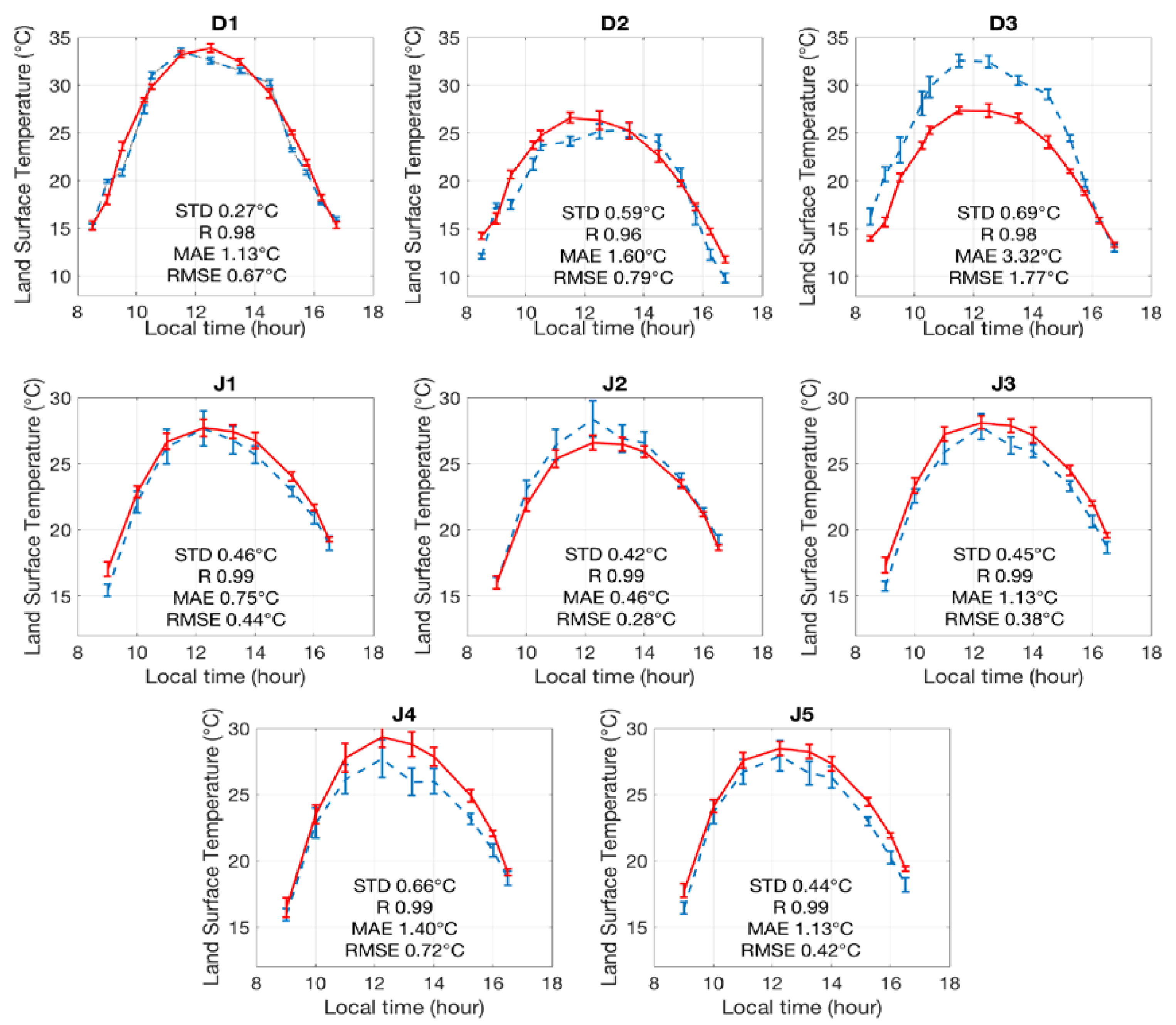
To examine the potential of UAVs to capture the diurnal cycle of LST and to evaluate the retrieval processing (e.g., georeferencing, mosaicking), we plot the retrieved temperatures for each of the conducted flights, together with the mean absolute error (MAE), root mean square error (RMSE) and correlation coefficient (R) of UAV-LST derived from comparison against in situ measurements (Figure 4). High correlation was observed between UAV-based and ground-based Apogee sensors (average of approx. 0.99 across all stations and campaigns). The MAE varied from 0.46 to 1.40 °C for the grass surface and from 1.13 to 3.32 °C for the harvested surface, while RMSE varied from 0.28 to 0.72 °C for the grass and from 0.67 to 1.77 °C for the harvested surface (see Figure 4). Relative to the January campaign, higher values of MAE and RMSE were found in December, particularly at Stations D2 and D3. This is likely related to the heterogeneity of the surface type, since the harvested maize field contains a mixed fraction of soil and vegetation observed within the Apogee FOV.
Differences between the UAV-based LST and the in situ Apogee measurements for all stations throughout the diurnal cycle are displayed in Figure 5. Overall the January campaign (J1–J5) showed a better agreement between the two datasets than in December (D1–D3). Differences range by up to 5 °C for December, while were generally less than 1.5 °C in January (except for Station J4, which has a maximum difference of −2.7 °C around 13:15). The diurnal response at J4 is likely due to the heterogeneity of the surface around the pivot track (location of J4), which can be considered as a mixed fraction of soil and vegetation. Interestingly, the MAE varies independently of the surface temperature throughout the day, demonstrating the capability of UAVs to retrieve LST with robustness across the diurnal cycle. The improved results for the grass surface type (J1–J5) are likely attributable to the relatively homogeneous surface within the Apogee FOV. Reinforcing this view is that the MAE and RMSE are similar for each station in January. Indeed, the December campaign indicated relatively high MAE compared to the January campaign. So, while results suggest that temperature differences are independent of the diurnal cycle, they vary with the underlying surface type. Overall, the diurnal UAV-based LST cycle shows good agreement with in situ measurements over the 8 comparisons stations. Importantly, a low RMSE (~0.7 °C) relative to the thermal camera error was determined, which improves upon the ±2 °C suggested by the manufacture based specifications [57,67].
3.2. Spatial Pattern of the Diurnal LST Cycle
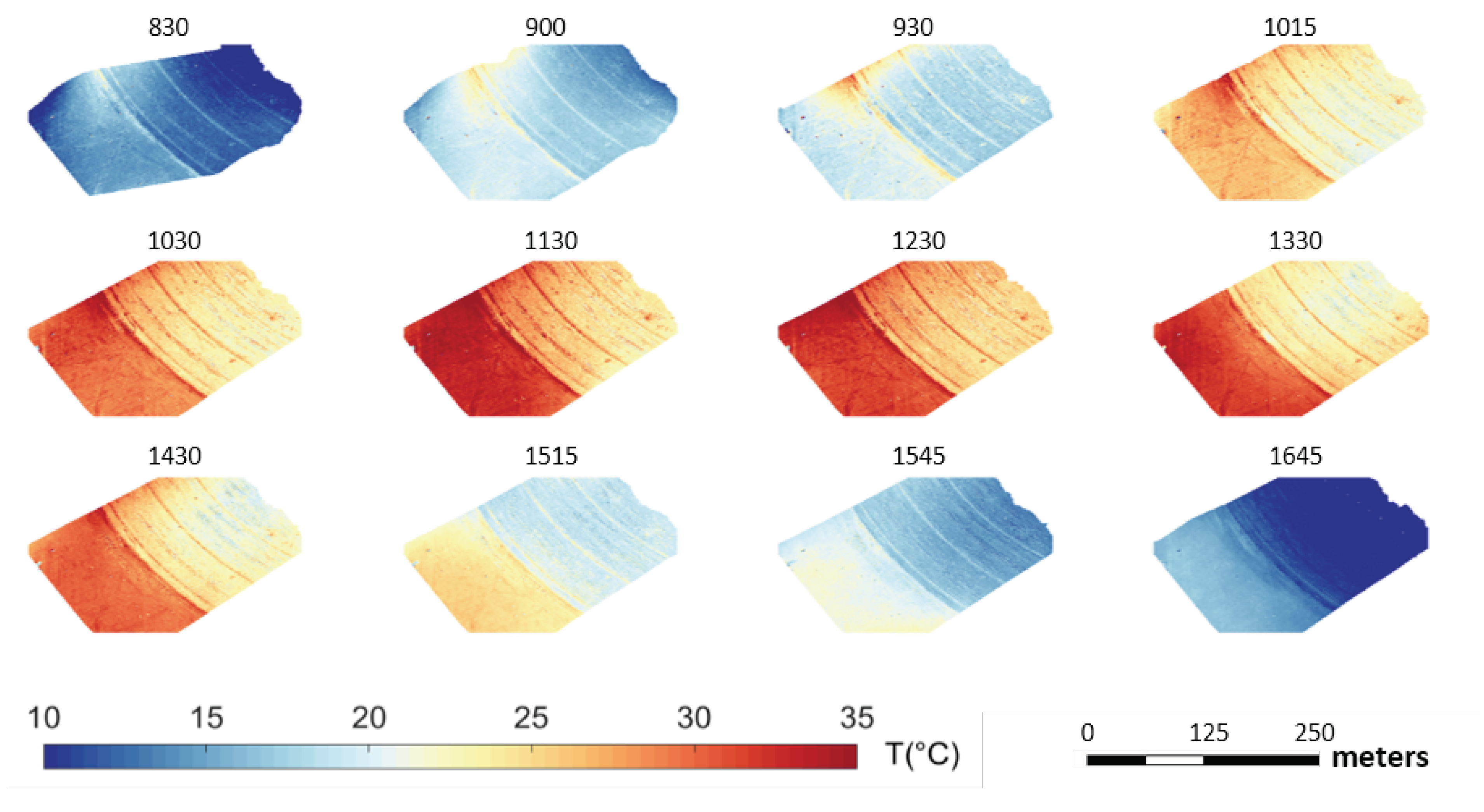
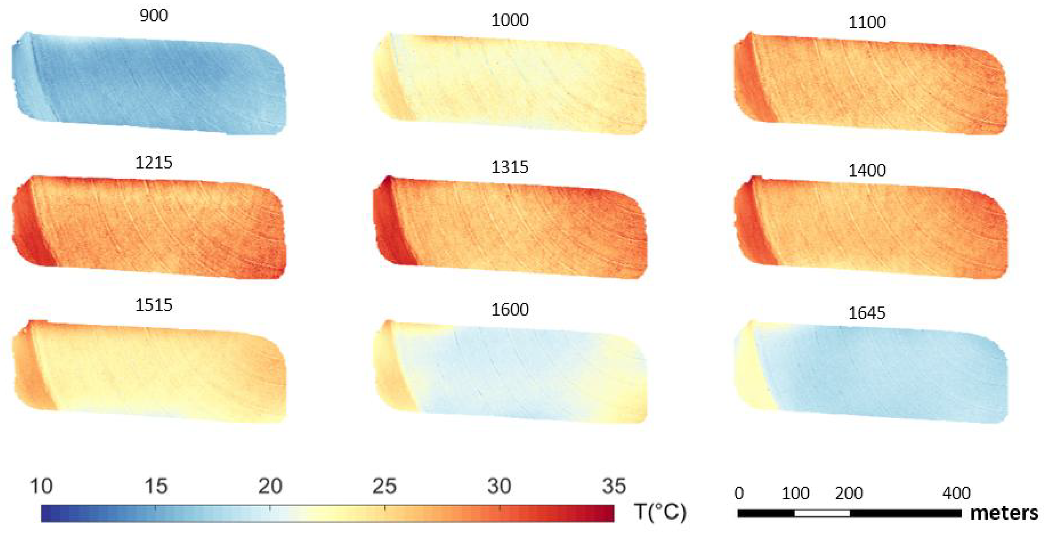
Figure 6 and Figure 7 show the diurnal LST maps for the desert/harvested field on 13 December (2016) and grass field on 31 January (2017), respectively. In both cases, it can be seen that the preliminary morning LST retrieval on each day varied only slightly across the relative surface types. However, as the surface heats up in response to an increasing amount of incident solar radiation (Figure 2), the LST climbs rapidly to reach the maximum temperature around solar noon. As expected, the LST over the desert was significantly higher than the LST over both the harvested maize (with residual weeds) and grass surfaces throughout the cycle, with a difference of approximately 4 °C (Figure 7), presumably caused by evaporative cooling. The land cover-based temperature differences were even more pronounced during the hottest periods of the day. For example, around 1 pm, the vegetation was about 6 °C cooler than the desert in December and 5 °C in January.
The differences between surface types remain constant until the last observation of the day at 1645. As can be seen from reference to Figure 2, the LST of the desert was much higher than the air temperature until around 1500. With no evaporative cooling process (given no moisture availability), the desert surface can only reemit the incident solar radiation as sensible heat. The lack of any moisture distribution within the desert reflects the greater spatially homogeneity, in contrast to the vegetation LST which was far more heterogeneous for any given observation time. While some anomalous high temperature pixels were observed close to the top edge of the image in several examples (0900 and 0930 in the December campaign, all of the January flights), these are the result of thermal mosaicking artefacts [43,46], rather than reflecting actual landscape features. To avoid the impacts of these border effects, only the central portions of the orthomosaic (visually no impacted by the border effects) are used in the statistical comparisons undertaken herein.
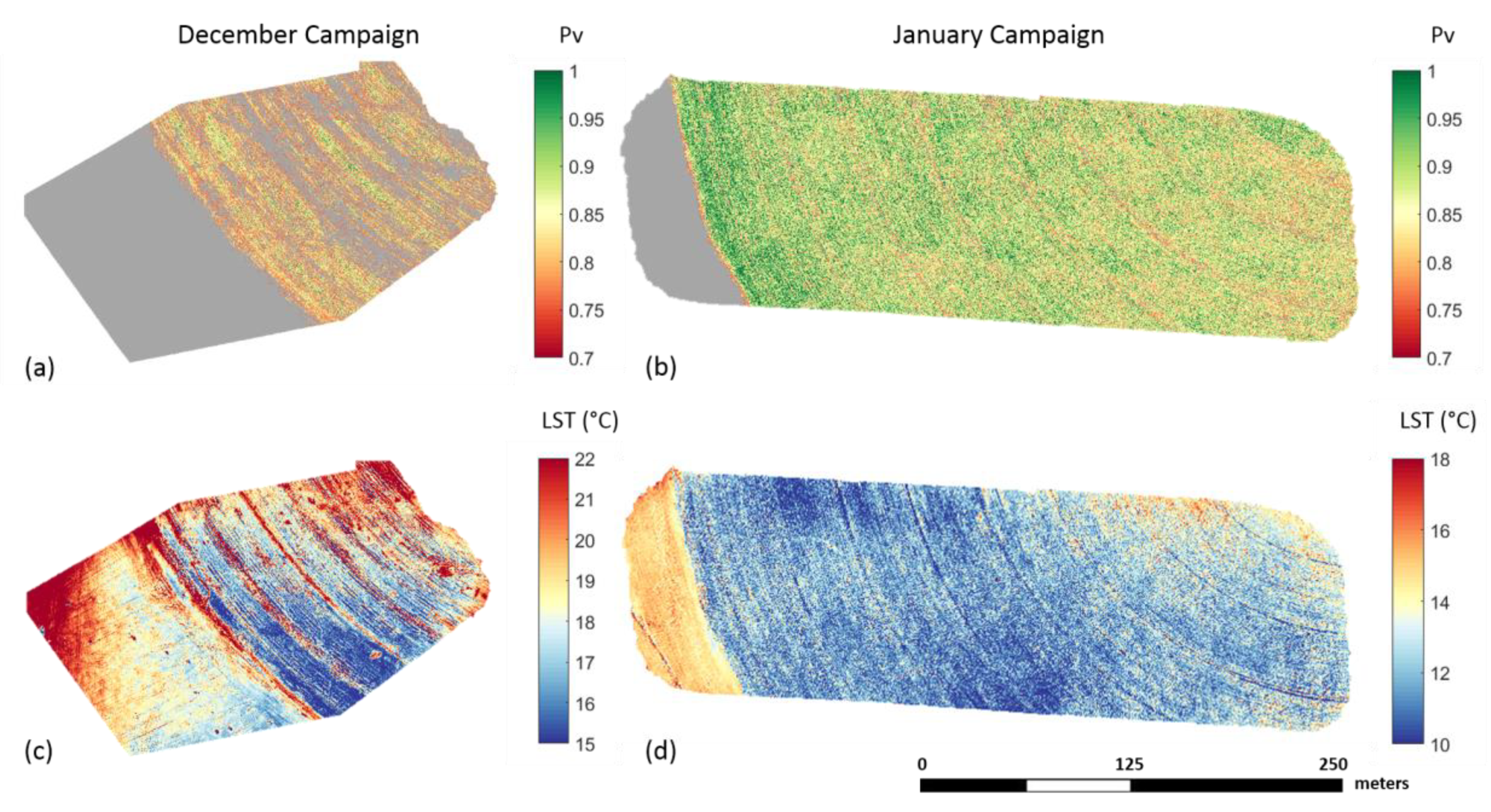
To investigate the LST variability across the studied surface combinations, the range (maximum-minimum) of LST on a per-pixel basis were computed for both the December and January campaigns (Figure 8). In both experiments, the diurnal range over the desert is greater than the other surface types. For both campaigns, the maximum LST was reached around solar noon (1150 and 1205, respectively) and was largely independent of the surface type in December. The heterogeneous surface surveyed in January saw small differences in the time maximum LST was observed, with earlier maximum LST observed for greater vegetation covers. Presumably, the vegetation and soil water status contribute to increased heat capacity, slowing down the warming of the surface in response to solar heating. Figure 8 shows the diurnal LST range is strongly related to surface type, with higher diurnal ranges for desert and bare soil surfaces, and lower diurnal ranges for vegetated surfaces. Within the center-pivot, differences in the diurnal range can be explained by the variable surface water status between the harvested maize and the grass fields. While the grass field was still being irrigated, the LST signature observed in the harvested field (no irrigation for more than 10 days) is likely due to residual moisture in the soil and in the mixture of weeds that remained in the field after harvesting (Figure 8). Given that surface water condition has a major influence on the morning rise of LST, the diurnal temperature range has been used as a signature of land surface fluxes and surface soil moisture status at daily scales [10,19].
To examine any potential changes in the spatial patterns of diurnal temperature relative to vegetation, the per-pixel LST was plotted against over the course of the diurnal cycle. As can be seen in Figure 9, distinct clusters represent the temperature distributions of the crop surface throughout the day. As expected, the harvested maize (a spread of 0.7 to 0.9) was lower than the grass (from 0.8 to 1). However, the harvested maize is relatively high considering the large part of bare soil in the field and this reveals the limitation of RGB to retrieve for this surface. In the following analysis, desert and bare soil surfaces have been excluded. There appears to be distinct phases corresponding to the rate of the rise and fall of the diurnal cycle presented in Figure 9. That is, the LST variability increases throughout the day until solar noon (described by the increasing height of the clusters) and then decreases towards sunset. The highest variability occurs around the peak of the maximum solar forcing during the day; inherent surface heterogeneities (e.g., soil texture, albedo, and water status) increase surface responses variability to the solar heating and thus provide larger LST variability [68]. Between 1000 and 1400, while the harvested maize presents greater variability independently of , the Rhodes grass surface presents a negative slope of LST relative to . The spatial patterns of the LST within the grass field clearly reflect the impact of evaporative cooling related to the vegetation condition, as explained by Moran el al. [69]. The evaporation associated with soil moisture would favor the partition of latent heat over sensible heat, and thus significantly reduce the diurnal amplitude of the LST cycle. In other word, an increase in green vegetation is often associated with a reduction in surface resistance to evapotranspiration, greater transpiration and a larger latent heat transfer resulting in lower LST. After 1400, LST variability starts to decrease, but with a different rate than the morning LST rise. The explanation for this asymmetry is possibly related to the difference in land surface feedbacks in the afternoon (such as a more stable surface-atmosphere interaction). At the end of the day, the distribution of LST over the grass field becomes uniform and varies independently of .
3.3. UAV-Based LST Comparison against Meteosat Second Generation-Spinning Enhanced Visible and Infrared Imager (MSG-SEVIRI) Retrievals
To investigate the potential of UAVs for improving evaluation strategies of coarse scale satellite derived retrievals, UAV-based LSTs were compared to the satellite-based LSTs obtained from the MSG-SEVIRI platform. The MSG-SEVIRI offers an independent method for analyzing the diurnal cycle and variability at large scales. However, since the MSG-LST resolution is coarse (3 km), the comparison is inevitably hindered by the considerable differences in scale (several orders of magnitude). In order to better understand the mixed-pixel LST response, we classified the land use within the MSG pixel into crop and desert using Sentinel 2 NDVI. Because each center pivot is enclosed by a surrounding desert, there is a sharp NDVI contrast between the land use types (i.e., we classified crop as NDVI ≥ 0.12 and desert as NDVI < 0.12). Approximately 84% of the MSG pixel was desert and/or bare soil for the December campaign, and 89% for the January campaign (with a second well irrigated pivot within the MSG pixel). Since NDVI was not directly retrievable from the UAV optical imagery, the surface type was classified based on the previously calculated estimates (Equation (5)). For the December campaign, 89% of UAV pixels were classified as desert or bare soil compared with only 23% for the January campaign. Given these values and the obvious differences in FOV between the MSG-SEVIRI and the UAV data, we averaged the UAV-based radiances (prior to LST retrieval) for three types of comparison: all UAV-based pixels, desert pixels only, and crop pixels only. In addition, a hypothetical LST was calculated to represent the temperature that the UAV-based LST would be if the same surface composition of the MSG pixel was maintained: i.e., , where is hypothetical LST, is the desert LST and is the crop LST. This hypothetical LST allows for a consistent comparison between MSG-based and UAV-based LST by taking into account the mixed-pixel response.
Figure 10 and Table 4 present the diurnal cycles and the statistics of the intercomparison between UAV-based and MSG-SEVIRI based LST for all pixels, desert pixels only, vegetation pixels only, and a hypothetical LST. As expected, given the strong diurnal variability, the UAV-based LST dynamic is statistically consistent with the MSG-SEVIRI based LST for both campaigns, with R values generally around 0.98–0.99. Given that the statistics are similar to those obtained in Section 3.1 and across both campaigns, it suggests that both evaluations are robust and consistent. MAE and RMSE are low and similar for both campaigns, with an MAE and an RMSE around 1 °C when excluding the results for the harvested maize surface type only. The MAE and RMSE were higher for the harvested maize surface type, a result of the MSG observing a much greater proportion of the desert (84%). However, the same response is not reflected for the grass surface in the January campaign. This apparent disparity can be explained by the MSG observing another pivot within the pixel that has a higher NDVI (approx. 0.30) than the NDVI observed in the UAV surveyed area (approx. 0.25). Consequently, the MSG-LST was impacted by the vegetation condition of this pivot (well-irrigated) compared to the pivot observed by UAV (i.e., wet vegetation appears colder than does dry vegetation). Thus, the MSG-LST appears slightly colder, and so the MAE for the grass surface type is lower than it would be if this other pivot was similar in vegetation conditions to the pivot being surveyed by the UAV. To assess the difference between UAV-based and MSG-based LST throughout the diurnal cycle, the bias between MSG-LST and the hypothetical-LST were computed across the day. The December campaign presents a bias of 1.7 °C, but these are again independent of the diurnal variation. The January campaign presents a bias that is systematically positive, varying between 0–1.7 °C. Once again, the slight overestimation of UAV-based LST can be explained by the second well irrigated pivot that is captured within the MSG pixel. The inter-comparison of the diurnal LST cycle allows for an assessment of the spatial and temporal consistency between UAV- and satellite-based LST. Regarding the agreement, it seems that the coarse-scale MSG-LST can offer some important insights into land surface condition that are consistent with ultra-high resolution UAV-based retrievals, at least in this particular environment.
4. Discussion
Recent developments in UAVs and lightweight thermal sensors have provided the capacity to observe, at ultra-high resolution, the spatial patterns of LST throughout the day. The results presented here indicate that these derived maps can identify the significant response differences between harvested maize, grass and desert surfaces. As vegetation cover (and fraction) increases, the diurnal LST variation decreases, as illustrated by the reduced heating of the grass relative to the other surface types. The grass surface showed diverse behavior due to the changing evaporative response throughout the day, while both the desert and harvested maize surfaces revealed similar diurnal LST variations that were likely due to the change in LST being constrained by the available water condition. In this latter case, any diurnal variation is likely a response to variations in solar heating, shading, soil thermal properties, and other related surface characteristics.
In comparing UAV-based LST to in situ measurements (see Figure 4), the RMSE was generally less than 0.7 °C over the grass surface and approximately 1.3 °C over others surfaces. LSTs have been retrieved at an accuracy of 2 °C or better, suggesting they have utility for surface flux retrieval [14,32]. The differences in MAE and RMSE can likely be related to the heterogeneity of the harvested maize surface (keeping in mind that there was only a single desert in situ station). Errors can also be introduced by the emissivity estimates over the different surface types (between 0.2 and 0.4 °C) [70]. For example, the harvested maize presents as a challenging surface type to estimate emissivity when only using vegetation fractional cover, as it is also influenced by surface features such as soil type and roughness [12,61] which are not easily. There are also sun-surface geometry effects that have not been included in this analysis, which may further impact the calculation of angular dependent surface emissivity and LST values [71]. Additional investigation on the effect of using different emissivity retrieval methods remains to be undertaken, as a relatively simple algorithm has been employed here due to a lack of more detailed surface data. Retrieval improvements for determining the emissivity are likely possible by incorporating near-infrared sensing (in addition to the thermal sensor) and correcting sun-view geometry effects via use of a digital elevation model within a 3D radiative transfer model. Cross-sensitivities between the thermal cameras retrieved temperature and environmental variables can also introduce systematic errors to the measured thermal radiation values. Temporal non-uniformity (i.e., a temperature-dependent drift problem) and spatial non-uniformity (e.g., vignette effect) are likely to require consideration, although relatively little literature currently exists on these effects [72].
Apart from errors associated with the LST retrieval and the UAV-thermal sensor itself, there are also errors related to the underlying structure from motion process used to construct the ortho-rectified UAV-based thermal maps. Studies have already reported that the SfM process struggles to stitch thermal images into an accurate orthomosaic [49,73], since these contain reduced information compared to RGB images, rendering the detection of common feature points more challenging. SfM is based on both the images position and also the capacity to match pixels for georeferencing and correcting image distortion. However, unlike RGB imagery, the LST can change rapidly during the course of the flight collection (as shown here), and the same pixel can be observed with different temperature depending on its position in the flight line (induced by the changing position of the sun and small-scale micro-meteorological impacts). As such, this will inevitably induce an error into the estimated diurnal LST response.
Irrespective of the numerous potential impacts on the accuracy of LST retrievals derived from satellite, UAV or ground based sensors, the UAV-based LST diurnal analysis revealed insights into surface response and behavior over this agricultural setting. For instance, the change in diurnal LST can provide insight into the timing of plant water use among highly heterogeneous landscapes, both natural and human-impacted. As mentioned by Fisher et al. [74], the deficiency of drought predictive capabilities is due in large part to missing information on land–atmosphere coupling i.e., evapotranspiration, and an under-emphasis on the response of vegetation to drought. Consequently, they recommend a need to resolve the diurnal cycle to support evapotranspiration responses and surface soil moisture status, and thus our knowledge on plant-water dynamics [75]. Moreover, monitoring of plant water status is critical not only for early detection of stress, but also to detect the diurnal irrigation deficit with the degree of precision needed [43]. Our findings highlight the potential to utilize diurnal UAV-based retrievals to enhance investigations in precision agriculture, detail hydrological processes at plant scale, and provide insights into coupled land–atmosphere studies. Importantly, UAV-based LST retrievals provide a new pathway to inform upon diurnal soil-vegetation-atmosphere processes and act as an intermediate resolution between ground measurement and larger scale data satellite data.
What is clear from this analysis at very high resolution is that even in relatively homogeneous conditions, LST can be quite variable in both space and time [76]. Indeed, this has made the evaluation of satellite-based retrievals particularly difficult. In heterogeneous cases, the evaluation of satellite products (such as MSG) requires extensive ground truthing, which is both costly and time consuming and, in many cases, limited to specific calibration/validation areas and selected periods. Evaluating LST from coarse-scale geostationary satellite data (or even moderate-resolution polar orbiting platforms) remains a major challenge [11], notably due to the large mismatch between the spatial resolution of spaceborne observations (3 km) and the representativeness scale (several cm) of localized in situ measurements. To help address the scaling issues and to circumvent the difficulties of direct comparison, we need approaches that bridge the gap between these incompatible scales. The direct intercomparison with diurnal LST derived from the MSG-SEVIRI product illustrated a high degree of consistency once the relative surface proportion within the MSG pixel were accounted for, revealing a promising approach for improving the evaluation strategies of coarse-scale satellite-based LST throughout the day. This analysis represents a first effort to compare diurnal satellite-based with UAV-based LST. While illustrating promise, further intercomparison studies need to be undertaken over more complex surfaces and for longer time periods than were examined in this preliminary investigation. With the recent launch of the ECOSTRESS mission, UAVs may provide a potential scaling tool to address the large disparity between the ~69 m cross-track by 38 m in-track spatial resolution and in situ station data. The ECOSTRESS mission aims to explore the terrestrial biosphere response (e.g., diurnal vegetation water stress) to changes in water availability by accurately measuring the temperature of plants. UAVs, by being able to fly low and on demand, could act to bridge the scaling gap between the fixed-point discrete ground-based observations and ECOSTRESS by providing within-pixel estimates of spatial and temporal variability, while offering the opportunity to better understand important scaling issues.
5. Conclusions
Rapid developments in UAV capabilities, particularly their ability to integrate miniaturized sensors, provides a unique opportunity to observe the diurnal cycle at an unprecedented spatial and temporal resolution. Here we present the first assessment of diurnal land surface temperature collected from an unmanned aerial vehicle, focusing on a number of different landcovers within a dryland agricultural setting. Analysis of the collected thermal imagery showed that the constructed LST maps reflect a strong diurnal cycle that is consistent with expected behavior, but with considerable spatial and temporal variability observed within and between the different landcovers. Results indicate that UAV-based LST are consistent with both ground-based and satellite measurements, with an RMSE of less than 1 °C. Numerous applications can benefit from information on the diurnal cycle of land surface temperature, including multi-disciplinary studies in agriculture, hydrology and land–atmosphere interactions. Furthermore, UAVs provide the opportunity for a new satellite evaluation strategy, by overcoming the point-scale limitation of in situ sensors. However, there remain a number of avenues requiring further examination, including: (1) sensor calibration, error characterization and spatiotemporal non-uniformity corrections; (2) retrieval algorithm improvements for emissivity impacts; (3) correcting LST for surface relief effects throughout the day (sun-angle geometry influence); (4) identifying in-flight effects (i.e., wind-speed and ambient temperature) on the stability of sensors and retrieval accuracy; and (5) quantifying the impact of post-processing software on the georectified surface temperature map. Overall, these results offer new insights into the dynamics of land surface behavior in both dry and wet soil conditions and at spatiotemporal scales that are unable to be replicated using traditional satellite platforms alone.
Author Contributions
The experimental design and methodology were conceived by S.P., B.A. and M.F.M. Data collection and the execution of the experiments was performed by S.P., B.A. and J.R. The project leadership was assumed by Y.M., who also analyzed the data and prepared the initial draft. All authors discussed the results and contributed to the development of the final manuscript.
Funding
The research reported in this publication was supported by the King Abdullah University of Science and Technology (KAUST).
Acknowledgments
We greatly appreciate the logistical, equipment and scientific support offered to our team by Jack King, Alan King and employees of the Tawdeehiya Farm in Al Kharj, Saudi Arabia, without whom this research would not have been possible.
Conflicts of Interest
The authors declare no conflict of interest.
References
- Anderson, M.; Norman, J.; Kustas, W.; Houborg, R.; Starks, P.; Agam, N. A thermal-based remote sensing technique for routine mapping of land-surface carbon, water and energy fluxes from field to regional scales. Remote Sens. Environ. 2008, 112, 4227–4241. [Google Scholar] [CrossRef]
- Brunsell, N.A.; Gillies, R.R. Length Scale Analysis of Surface Energy Fluxes Derived from Remote Sensing. J. Hydrometeorol. 2003, 4, 1212–1219. [Google Scholar] [CrossRef] [Green Version]
- Karnieli, A.; Agam, N.; Pinker, R.T.; Anderson, M.; Imhoff, M.L.; Gutman, G.G.; Panov, N.; Goldberg, A. Use of NDVI and Land Surface Temperature for Drought Assessment: Merits and Limitations. J. Clim. 2010, 23, 618–633. [Google Scholar] [CrossRef]
- Kustas, W.; Anderson, M. Advances in thermal infrared remote sensing for land surface modeling. Agric. For. Meteorol. 2009, 149, 2071–2081. [Google Scholar] [CrossRef]
- Kerr, Y.H.; Lagouarde, J.P.; Nerry, F.; Ottlé, C. Land Surface Temperature Retrieval Techniques and Applications; CRC Press: Boston, MA, USA, 2004. [Google Scholar]
- WMO. Systematic Observation Requirements for Satellite-Based Data Products for Climate—2011 Update; WMO: Geneva, Switzerland, 2011; Volume 127. [Google Scholar]
- Townshend, J.; Justice, C.; Skole, D.; Malingreau, J.-P.; Cihlar, J.; Teillet, P.; Sadowski, F.; Ruttenberg, S. The 1 km resolution global data set: Needs of the International Geosphere Biosphere Programme†. Int. J. Remote Sens. 1994, 15, 3417–3441. [Google Scholar] [CrossRef]
- Carlson, T.N.; Boland, F.E. Analysis of Urban-Rural Canopy Using a Surface Heat Flux/Temperature Model. J. Appl. Meteorol. 1978, 17, 998–1013. [Google Scholar] [CrossRef] [Green Version]
- Price, J.C. On the analysis of thermal infrared imagery: The limited utility of apparent thermal inertia. Remote Sens. Environ. 1985, 18, 59–73. [Google Scholar] [CrossRef]
- Wetzel, P.J.; Atlas, D.; Woodward, R.H. Determining Soil Moisture from Geosynchronous Satellite Infrared Data: A Feasibility Study. J. Clim. Appl. Meteorol. 1984, 23, 375–391. [Google Scholar] [CrossRef] [Green Version]
- Prata, A.J.; Caselles, V.; Coll, C.; Sobrino, J.A.; Ottlé, C. Thermal remote sensing of land surface temperature from satellites: Current status and future prospects. Remote Sens. Rev. 1995, 12, 175–224. [Google Scholar] [CrossRef]
- Sobrino, J.A.; Jimenez-Muoz, J.C.; Soria, G.; Romaguera, M.; Guanter, L.; Moreno, J.; Plaza, A.; Martinez, P. Land Surface Emissivity Retrieval From Different VNIR and TIR Sensors. IEEE Trans. Geosci. Remote Sens. 2008, 46, 316–327. [Google Scholar] [CrossRef]
- Gillespie, A.; Rokugawa, S.; Matsunaga, T.; Steven Cothern, J.; Hook, S.; Kahle, A.B. A temperature and emissivity separation algorithm for advanced spaceborne thermal emission and reflection radiometer (ASTER) images. IEEE Trans. Geosci. Remote Sens. 1998, 36, 1113–1126. [Google Scholar] [CrossRef]
- Wan, Z.; Dozier, J. A generalized split-window algorithm for retrieving land-surface temperature from space. IEEE Trans. Geosci. Remote Sens. 1996, 34, 892–905. [Google Scholar] [CrossRef]
- Koch, J.; Siemann, A.; Stisen, S.; Sheffield, J. Spatial validation of large-scale land surface models against monthly land surface temperature patterns using innovative performance metrics. J. Geophys. Res. Atmos. 2016, 121, 5430–5452. [Google Scholar] [CrossRef] [Green Version]
- Zink, M.; Mai, J.; Cuntz, M.; Samaniego, L. Conditioning a Hydrologic Model Using Patterns of Remotely Sensed Land Surface Temperature. Water Resour. Res. 2018, 2976–2998. [Google Scholar] [CrossRef]
- Stisen, S.; McCabe, M.F.; Refsgaard, J.C.; Lerer, S.; Butts, M.B. Model parameter analysis using remotely sensed pattern information in a multi-constraint framework. J. Hydrol. 2011, 409, 337–349. [Google Scholar] [CrossRef]
- McCabe, M.F.; Franks, S.W.; Kalma, J.D. Calibration of a land surface model using multiple data sets. J. Hydrol. 2005, 302, 209–222. [Google Scholar] [CrossRef]
- Anderson, M. A Two-Source Time-Integrated Model for Estimating Surface Fluxes Using Thermal Infrared Remote Sensing. Remote Sens. Environ. 1997, 60, 195–216. [Google Scholar] [CrossRef]
- Anderson, M.C.; Allen, R.G.; Morse, A.; Kustas, W.P. Use of Landsat thermal imagery in monitoring evapotranspiration and managing water resources. Remote Sens. Environ. 2012, 122, 50–65. [Google Scholar] [CrossRef]
- Sun, Z.; Gebremichael, M.; Ardö, J.; Nickless, A.; Caquet, B.; Merboldh, L.; Kutschi, W. Estimation of daily evapotranspiration over Africa using MODIS/Terra and SEVIRI/MSG data. Atmos. Res. 2012, 112, 35–44. [Google Scholar] [CrossRef]
- Petropoulos, G.P.; Ireland, G.; Lamine, S.; Griffiths, H.M.; Ghilain, N.; Anagnostopoulos, V.; North, M.R.; Srivastava, P.K.; Georgopoulou, H. Operational evapotranspiration estimates from SEVIRI in support of sustainable water management. Int. J. Appl. Earth Obs. Geoinf. 2016, 49, 175–187. [Google Scholar] [CrossRef]
- Zhao, W.; Li, Z.-L. Sensitivity study of soil moisture on the temporal evolution of surface temperature over bare surfaces. Int. J. Remote Sens. 2013, 34, 3314–3331. [Google Scholar] [CrossRef]
- Piles, M.; Petropoulos, G.P.; Sánchez, N.; González-Zamora, Á.; Ireland, G. Towards improved spatio-temporal resolution soil moisture retrievals from the synergy of SMOS and MSG SEVIRI spaceborne observations. Remote Sens. Environ. 2016, 180, 403–417. [Google Scholar] [CrossRef] [Green Version]
- Fensholt, R.; Sandholt, I.; Stisen, S.; Tucker, C. Analysing NDVI for the African continent using the geostationary meteosat second generation SEVIRI sensor. Remote Sens. Environ. 2006, 101, 212–229. [Google Scholar] [CrossRef]
- Coudert, B.; Ottlé, C.; Briottet, X. Monitoring land surface processes with thermal infrared data: Calibration of SVAT parameters based on the optimisation of diurnal surface temperature cycling features. Remote Sens. Environ. 2008, 112, 872–887. [Google Scholar] [CrossRef]
- Duan, S.-B.; Li, Z.-L.; Tang, B.-H.; Wu, H.; Tang, R.; Bi, Y.; Zhou, G. Estimation of Diurnal Cycle of Land Surface Temperature at High Temporal and Spatial Resolution from Clear-Sky MODIS Data. Remote Sens. 2014, 6, 3247–3262. [Google Scholar] [CrossRef] [Green Version]
- Wang, J.; Bras, R. Ground heat flux estimated from surface soil temperature. J. Hydrol. 1999, 216, 214–226. [Google Scholar] [CrossRef]
- Zhu, W.; Wu, B.; Yan, N.; Feng, X.; Xing, Q. A method to estimate diurnal surface soil heat flux from MODIS data for a sparse vegetation and bare soil. J. Hydrol. 2014, 511, 139–150. [Google Scholar] [CrossRef]
- Zhou, J.; Chen, Y.; Zhang, X.; Zhan, W. Modelling the diurnal variations of urban heat islands with multi-source satellite data. Int. J. Remote Sens. 2013, 34, 7568–7588. [Google Scholar] [CrossRef]
- Santanello, J.A.; Friedl, M.A. Diurnal Covariation in Soil Heat Flux and Net Radiation. J. Appl. Meteorol. 2003, 42, 851–862. [Google Scholar] [CrossRef]
- Li, Z.L.; Tang, B.H.; Wu, H.; Ren, H.; Yan, G.; Wan, Z.; Trigo, I.F.; Sobrino, J.A. Satellite-derived land surface temperature: Current status and perspectives. Remote Sens. Environ. 2013, 131, 14–37. [Google Scholar] [CrossRef] [Green Version]
- Sobrino, J.A.; Del Frate, F.; Drusch, M.; Jiménez-Muñoz, J.C.; Manunta, P.; Regan, A. Review of thermal infrared applications and requirements for future high-resolution sensors. IEEE Trans. Geosci. Remote Sens. 2016, 54, 2963–2972. [Google Scholar] [CrossRef]
- Fisher, J.B.; Hook, S.J.; Allen, R.G.; Anderson, M.C.; French, A.N.; Hain, C.; Hulley, G.C.; Wood, E.F. ECOSTRESS: NASA’s next-generation mission to measure evapotranspiration from the International Space Station. In Proceedings of the AGU Fall Meeting Abstracts, San Francisco, CA, USA, 14–18 December 2015. [Google Scholar]
- Weng, Q. Thermal infrared remote sensing for urban climate and environmental studies: Methods, applications, and trends. ISPRS J. Photogramm. Remote Sens. 2009, 64, 335–344. [Google Scholar] [CrossRef]
- McCabe, M.F.; Rodell, M.; Alsdorf, D.E.; Miralles, D.G.; Uijlenhoet, R.; Wagner, W.; Lucieer, A.; Houborg, R.; Verhoest, N.E.C.; Franz, T.E.; et al. The future of Earth observation in hydrology. Hydrol. Earth Syst. Sci. 2017, 21, 3879–3914. [Google Scholar] [CrossRef] [Green Version]
- Vasterling, M.; Meyer, U. Challenges and Opportunities for UAV-Borne Thermal Imaging. In Thermal Infrared Remote Sensing: Sensors, Methods, Applications; Kuenzer, C., Dech, S., Eds.; Springer Netherlands: Dordrecht, The Netherlands, 2013; pp. 69–92. ISBN 978-94-007-6639-6. [Google Scholar]
- Manfreda, S.; McCabe, M.; Miller, P.; Lucas, R.; Pajuelo Madrigal, V.; Mallinis, G.; Ben Dor, E.; Helman, D.; Estes, L.; Ciraolo, G.; et al. On the Use of Unmanned Aerial Systems for Environmental Monitoring. Remote Sens. 2018, 10, 641. [Google Scholar] [CrossRef]
- Jagt, B.; Lucieer, A.; Wallace, L.; Turner, D.; Durand, M. Snow Depth Retrieval with UAS Using Photogrammetric Techniques. Geosciences 2015, 5, 264–285. [Google Scholar] [CrossRef]
- Marti, R.; Gascoin, S.; Berthier, E.; de Pinel, M.; Houet, T.; Laffly, D. Mapping snow depth in open alpine terrain from stereo satellite imagery. Cryosphere 2016, 10, 1361–1380. [Google Scholar] [CrossRef] [Green Version]
- Perks, M.T.; Russell, A.J.; Large, A.R.G. Technical Note: Advances in flash flood monitoring using unmanned aerial vehicles (UAVs). Hydrol. Earth Syst. Sci. 2016, 20, 4005–4015. [Google Scholar] [CrossRef]
- D’Oleire-Oltmanns, S.; Marzolff, I.; Peter, K.D.; Ries, J.B. Unmanned aerial vehicle (UAV) for monitoring soil erosion in Morocco. Remote Sens. 2012, 4, 3390–3416. [Google Scholar] [CrossRef]
- Zhang, C.; Kovacs, J.M. The application of small unmanned aerial systems for precision agriculture: A review. Precis. Agric. 2012, 13, 693–712. [Google Scholar] [CrossRef]
- Zarco-Tejada, P.J.; González-Dugo, V.; Berni, J.A.J. Fluorescence, temperature and narrow-band indices acquired from a UAV platform for water stress detection using a micro-hyperspectral imager and a thermal camera. Remote Sens. Environ. 2012, 117, 322–337. [Google Scholar] [CrossRef] [Green Version]
- Zarco-Tejada, P.J.; Guillén-Climent, M.L.; Hernández-Clemente, R.; Catalina, A.; González, M.R.; Martín, P. Estimating leaf carotenoid content in vineyards using high resolution hyperspectral imagery acquired from an unmanned aerial vehicle (UAV). Agric. For. Meteorol. 2013, 171–172, 281–294. [Google Scholar] [CrossRef]
- Calderón, R.; Navas-Cortés, J.A.; Lucena, C.; Zarco-Tejada, P.J. High-resolution airborne hyperspectral and thermal imagery for early detection of Verticillium wilt of olive using fluorescence, temperature and narrow-band spectral indices. Remote Sens. Environ. 2013, 139, 231–245. [Google Scholar] [CrossRef] [Green Version]
- Gonzalez-Dugo, V.; Zarco-Tejada, P.; Nicolás, E.; Nortes, P.A.; Alarcón, J.J.; Intrigliolo, D.S.; Fereres, E. Using high resolution UAV thermal imagery to assess the variability in the water status of five fruit tree species within a commercial orchard. Precis. Agric. 2013, 14, 660–678. [Google Scholar] [CrossRef]
- Gonzalez-Dugo, V.; Zarco-Tejada, P.J.; Fereres, E. Applicability and limitations of using the crop water stress index as an indicator of water deficits in citrus orchards. Agric. For. Meteorol. 2014, 198–199, 94–104. [Google Scholar] [CrossRef]
- Baluja, J.; Diago, M.P.; Balda, P.; Zorer, R.; Meggio, F.; Morales, F.; Tardaguila, J. Assessment of vineyard water status variability by thermal and multispectral imagery using an unmanned aerial vehicle (UAV). Irrig. Sci. 2012, 30, 511–522. [Google Scholar] [CrossRef] [Green Version]
- Hoffmann, H.; Nieto, H.; Jensen, R.; Guzinski, R.; Zarco-Tejada, P.; Friborg, T. Estimating evaporation with thermal UAV data and two-source energy balance models. Hydrol. Earth Syst. Sci. 2016, 20, 697–713. [Google Scholar] [CrossRef] [Green Version]
- Ortega-Farías, S.; Ortega-Salazar, S.; Poblete, T.; Kilic, A.; Allen, R.; Poblete-Echeverría, C.; Ahumada-Orellana, L.; Zuñiga, M.; Sepúlveda, D. Estimation of Energy Balance Components over a Drip-Irrigated Olive Orchard Using Thermal and Multispectral Cameras Placed on a Helicopter-Based Unmanned Aerial Vehicle (UAV). Remote Sens. 2016, 8, 638. [Google Scholar] [CrossRef]
- Sullivan, D.G.; Fulton, J.P.; Shaw, J.N.; Bland, G. Evaluating the Sensitivity of an Unmanned Thermal Infrared Aerial System to Detect Water Stress in a Cotton Canopy. Trans. ASABE 2007, 50, 1963–1969. [Google Scholar] [CrossRef]
- Berni, J.; Zarco-Tejada, P.J.; Suarez, L.; Fereres, E. Thermal and Narrowband Multispectral Remote Sensing for Vegetation Monitoring From an Unmanned Aerial Vehicle. IEEE Trans. Geosci. Remote Sens. 2009, 47, 722–738. [Google Scholar] [CrossRef] [Green Version]
- Westoby, M.J.; Brasington, J.; Glasser, N.F.; Hambrey, M.J.; Reynolds, J.M. “Structure-from-Motion” photogrammetry: A low-cost, effective tool for geoscience applications. Geomorphology 2012, 179, 300–314. [Google Scholar] [CrossRef] [Green Version]
- Rosas, J.; Houborg, R.; McCabe, M.F. Sensitivity of Landsat 8 Surface Temperature Estimates to Atmospheric Profile Data: A Study Using MODTRAN in Dryland Irrigated Systems. Remote Sens. 2017, 9, 988. [Google Scholar] [CrossRef]
- Maes, W.H.; Steppe, K. Estimating evapotranspiration and drought stress with ground-based thermal remote sensing in agriculture: A review. J. Exp. Bot. 2012, 63, 4671–4712. [Google Scholar] [CrossRef] [PubMed]
- Berdahl, P.; Fromberg, R. The thermal radiance of clear skies. Sol. Energy 1982, 29, 299–314. [Google Scholar] [CrossRef]
- Maes, W.; Huete, A.; Steppe, K. Optimizing the Processing of UAV-Based Thermal Imagery. Remote Sens. 2017, 9, 476. [Google Scholar] [CrossRef]
- Park, S.; Ryu, D.; Fuentes, S.; Chung, H.; Hernández-Montes, E.; O’Connell, M. Adaptive estimation of crop water stress in nectarine and peach orchards using high-resolution imagery from an unmanned aerial vehicle (UAV). Remote Sens. 2017, 9. [Google Scholar] [CrossRef]
- Jones, H.G. Use of infrared thermography for monitoring stomatal closure in the field: Application to grapevine. J. Exp. Bot. 2002, 53, 2249–2260. [Google Scholar] [CrossRef] [PubMed]
- Jones, H.G.; Archer, N.; Rotenberg, E.; Casa, R. Radiation measurement for plant ecophysiology. J. Exp. Bot. 2003, 54, 879–889. [Google Scholar] [CrossRef] [PubMed] [Green Version]
- Li, Z.-L.; Wu, H.; Wang, N.; Qiu, S.; Sobrino, J.A.; Wan, Z.; Tang, B.-H.; Yan, G. Land surface emissivity retrieval from satellite data. Int. J. Remote Sens. 2013, 34, 3084–3127. [Google Scholar] [CrossRef]
- Sobrino, J.A.; Raissouni, N. Toward remote sensing methods for land cover dynamic monitoring: Application to Morocco. Int. J. Remote Sens. 2000, 21, 353–366. [Google Scholar] [CrossRef]
- Ogawa, K.; Schmugge, T. Mapping Surface Broadband Emissivity of the Sahara Desert Using ASTER and MODIS Data. Earth Interact. 2004, 8, 1–14. [Google Scholar] [CrossRef]
- Gitelson, A.A.; Kaufman, Y.J.; Stark, R.; Rundquist, D. Novel algorithms for remote estimation of vegetation fraction. Remote Sens. Environ. 2002, 80, 76–87. [Google Scholar] [CrossRef] [Green Version]
- Motohka, T.; Nasahara, K.N.; Oguma, H.; Tsuchida, S. Applicability of Green-Red Vegetation Index for Remote Sensing of Vegetation Phenology. Remote Sens. 2010, 2, 2369–2387. [Google Scholar] [CrossRef] [Green Version]
- Göttsche, F.M.; Olesen, F.S.; Bork-Unkelbach, A. Validation of land surface temperature derived from MSG/SEVIRI with in situ measurements at Gobabeb, Namibia. Int. J. Remote Sens. 2013, 34, 3069–3083. [Google Scholar] [CrossRef]
- Ball, M.; Pinkerton, H. Factors affecting the accuracy of thermal imaging cameras in volcanology. J. Geophys. Res. Solid Earth 2006, 111, 1–14. [Google Scholar] [CrossRef]
- Gentine, P.; Entekhabi, D.; Polcher, J. The Diurnal Behavior of Evaporative Fraction in the Soil–Vegetation–Atmospheric Boundary Layer Continuum. J. Hydrometeorol. 2011, 12, 1530–1546. [Google Scholar] [CrossRef] [Green Version]
- Moran, M.S.; Clarke, T.R.; Inoue, Y.; Vidal, A. Estimating crop water deficit using the relation between surface-air temperature and spectral vegetation index. Remote Sens. Environ. 1994, 49, 246–263. [Google Scholar] [CrossRef]
- Jiménez-Muñoz, J.C.; Sobrino, J.A. Error sources on the land surface temperature retrieved from thermal infrared single channel remote sensing data. Int. J. Remote Sens. 2006, 27, 999–1014. [Google Scholar] [CrossRef]
- Malbéteau, Y.; Merlin, O.; Gascoin, S.; Gastellu, J.P.; Mattar, C.; Olivera-Guerra, L.; Khabba, S.; Jarlan, L. Normalizing land surface temperature data for elevation and illumination effects in mountainous areas: A case study using ASTER data over a steep-sided valley in Morocco. Remote Sens. Environ. 2017, 189. [Google Scholar] [CrossRef]
- Smigaj, M.; Gaulton, R.; Suarez, J.C.; Barr, S.L. Use of miniature thermal cameras for detection of physiological stress in conifers. Remote Sens. 2017, 9. [Google Scholar] [CrossRef]
- Pech, K.; Stelling, N.; Karrasch, P.; Maas, H.-G. Generation of multitemporal thermal orthophotos from uav data. Int. Arch. Photogramm. Remote Sens. Spat. Inf. Sci. 2013, 1, 305–310. [Google Scholar] [CrossRef]
- Fisher, J.B.; Melton, F.; Middleton, E.; Hain, C.; Anderson, M.; Allen, R.; Mccabe, M.F.; Hook, S.; Baldocchi, D.; Townsend, P.A.; et al. The future of evapotranspiration: Global requirements for ecosystemfunctioning, carbon and climate feedbacks, agriculturalmanagement, and water resources. Water Resour. Res. 2017, 10.1002/20, 2618–2626. [Google Scholar] [CrossRef]
- Leinonen, I.; Grant, O.M.; Tagliavia, C.P.P.; Chaves, M.M.; Jones, H.G. Estimating stomatal conductance with thermal imagery. Plant Cell Environ. 2006, 29, 1508–1518. [Google Scholar] [CrossRef] [PubMed] [Green Version]
- McCabe, M.F.; Balick, L.K.; Theiler, J.; Gillespie, A.R.; Mushkin, A. Linear mixing in thermal infrared temperature retrieval. Int. J. Remote Sens. 2008, 29, 5047–5061. [Google Scholar] [CrossRef]
Figure 1.
The Tawdeehiya farm and the two focus areas where unmanned aerial vehicle (UAV) surveys were conducted on 13 December 2016 (a) and 31 January 2017 (b).
Figure 1.
The Tawdeehiya farm and the two focus areas where unmanned aerial vehicle (UAV) surveys were conducted on 13 December 2016 (a) and 31 January 2017 (b).

Figure 2.
Diurnal variations of net radiation (blue line) and air temperature (red line) at the meteorological station for 13 December 2016 (a) and 31 January 2017 (b).
Figure 2.
Diurnal variations of net radiation (blue line) and air temperature (red line) at the meteorological station for 13 December 2016 (a) and 31 January 2017 (b).

Figure 3.
Standard deviation of diurnal UAV-based land surface temperature (LST) within 9 × 9 pixels (90 × 90 cm) (a,c) and Apogee field-of-view (FOV) windows (b,d) for the 3 stations (D1–D3) on 13 December 2016 and for the 5 stations (J1–J5) on 31 January 2017.
Figure 3.
Standard deviation of diurnal UAV-based land surface temperature (LST) within 9 × 9 pixels (90 × 90 cm) (a,c) and Apogee field-of-view (FOV) windows (b,d) for the 3 stations (D1–D3) on 13 December 2016 and for the 5 stations (J1–J5) on 31 January 2017.

Figure 4.
Diurnal cycle of UAV-based LST (blue dashed line) versus in situ temperature as measured by Apogee sensors (red line) for the December (D1–D3) and January (J1–J5) campaigns, along with statistics including the in situ LST standard deviation (STD), correlation coefficient (R), mean absolute error (MAE) and root mean square error (RMSE).

Figure 5.
Diurnal temperature difference between UAV-based and in situ measurements for the December (a) and January campaigns (b).
Figure 5.
Diurnal temperature difference between UAV-based and in situ measurements for the December (a) and January campaigns (b).

Figure 6.
Maps of the UAV-based LST between 0830 and 1645 on 13 December 2016.

Figure 7.
Maps of the UAV-based LST between 0900 and 1645 on 31 January 2017.

Figure 8.
Maps of the proportion vegetation (a,b) estimated by using red–green–blue (RGB) camera and the range of diurnal LST (c,d) for the December campaign (a,c) and January Campaign (b,d). Grey areas are considered as desert or bare soil surfaces.
Figure 8.
Maps of the proportion vegetation (a,b) estimated by using red–green–blue (RGB) camera and the range of diurnal LST (c,d) for the December campaign (a,c) and January Campaign (b,d). Grey areas are considered as desert or bare soil surfaces.

Figure 9.
Diurnal cycles of pixel-based LST versus proportion of vegetation () between 830 and 1645 on 13 December 2016 (a) and 31 January 2017 (b). Distinct clusters represent the temperature distributions for each flight.
Figure 9.
Diurnal cycles of pixel-based LST versus proportion of vegetation () between 830 and 1645 on 13 December 2016 (a) and 31 January 2017 (b). Distinct clusters represent the temperature distributions for each flight.

Figure 10.
Diurnal Meteosat Second Generation (MSG)-based LST, UAV-based LST for all observed pixels (with error bars corresponding to standard deviation), UAV-based LST for desert pixels only, UAV-based LST for pivot pixels only, and hypothetical LST during (a) the December and (b) the January campaigns.


Table 1.
Flight characteristics and meteorological conditions for the 13 December 2016 campaign.
| Flight Details | 1 | 2 | 3 | 4 | 5 | 6 | 7 | 8 | 9 | 10 | 11 | 12 |
|---|---|---|---|---|---|---|---|---|---|---|---|---|
| Time of flight | 830 | 850 | 930 | 1015 | 1035 | 1130 | 1230 | 1330 | 1430 | 1515 | 1545 | 1645 |
| Images Used | 766 | 767 | 442 | 453 | 444 | 451 | 457 | 463 | 458 | 450 | 455 | 490 |
| Air Temp (°C) | 11.3 | 12.7 | 14.5 | 16.4 | 17.1 | 18.8 | 20.5 | 21.5 | 22.2 | 22.1 | 21.9 | 20 |
| Wind (m/s) | 1 | 1.2 | 0.8 | 0.6 | 0.7 | 1.2 | 1.1 | 1.8 | 1.9 | 2.1 | 2.4 | 2.5 |
| Direction | W | NW | NW | N | NE | SE | SE | SE | S | S | SE | SE |
Table 2.
Flight characteristics and meteorological conditions for 31 January 2017 campaign.
| Flight Details | 1 | 2 | 3 | 4 | 5 | 6 | 7 | 8 | 9 |
|---|---|---|---|---|---|---|---|---|---|
| Time of flight | 900 | 1005 | 1105 | 1210 | 1315 | 1405 | 1510 | 1600 | 1640 |
| Images Used | 1208 | 1212 | 1211 | 1215 | 1212 | 1210 | 1213 | 1210 | 1205 |
| Air Temp (°C) | 14 | 16.4 | 18.4 | 20.4 | 22.4 | 22.8 | 23.4 | 23.2 | 22.5 |
| Wind (m/s) | 3.6 | 4.4 | 4.7 | 5.4 | 6.2 | 6.5 | 5.9 | 5.6 | 4.7 |
| Direction | SE | SE | S | S | S | S | S | S | S |
Table 3.
Correction for Apogee infrared radiometer equations based on y = mx + b, where y is the calibrated Apogee, m is the slope, x is the uncorrected Apogee temperature, and b is the intercept.
Table 3.
Correction for Apogee infrared radiometer equations based on y = mx + b, where y is the calibrated Apogee, m is the slope, x is the uncorrected Apogee temperature, and b is the intercept.
| Apogee Sensor | D1/J1 | J2 | J3 | D2/J4 | D3/J5 |
|---|---|---|---|---|---|
| Slope | 1.05 | 1.00 | 0.99 | 1.02 | 1.04 |
| Intercept | 2.76 | 3.53 | 3.82 | 3.30 | 3.10 |
Table 4.
An intercomparison between UAV-based and MSG-Spinning Enhanced Visible and Infrared Imager (SEVIRI) based LST for all pixels, desert pixels only, vegetation pixels only, and a hypothetical LST. R is the correlation coefficient, MAE is the mean bias and RMSE is the root mean square error.
Table 4.
An intercomparison between UAV-based and MSG-Spinning Enhanced Visible and Infrared Imager (SEVIRI) based LST for all pixels, desert pixels only, vegetation pixels only, and a hypothetical LST. R is the correlation coefficient, MAE is the mean bias and RMSE is the root mean square error.
| Campaign | Surface Type | R | MAE (°C) | RMSE (°C) |
|---|---|---|---|---|
| December | all pixels | 0.99 | 0.85 | 1.07 |
| harvested | 0.96 | 2.24 | 2.56 | |
| desert | 0.99 | 1.04 | 1.25 | |
| hypothetical | 0.98 | 0.87 | 1.13 | |
| January | all pixels | 0.98 | 0.66 | 0.76 |
| grass | 0.98 | 0.88 | 0.97 | |
| desert | 0.98 | 0.94 | 1.11 | |
| hypothetical | 0.99 | 0.78 | 0.98 |
© 2018 by the authors. Licensee MDPI, Basel, Switzerland. This article is an open access article distributed under the terms and conditions of the Creative Commons Attribution (CC BY) license (http://creativecommons.org/licenses/by/4.0/).
Share and Cite
MDPI and ACS Style
Malbéteau, Y.; Parkes, S.; Aragon, B.; Rosas, J.; McCabe, M.F. Capturing the Diurnal Cycle of Land Surface Temperature Using an Unmanned Aerial Vehicle. Remote Sens. 2018, 10, 1407. https://0-doi-org.brum.beds.ac.uk/10.3390/rs10091407
AMA Style
Malbéteau Y, Parkes S, Aragon B, Rosas J, McCabe MF. Capturing the Diurnal Cycle of Land Surface Temperature Using an Unmanned Aerial Vehicle. Remote Sensing. 2018; 10(9):1407. https://0-doi-org.brum.beds.ac.uk/10.3390/rs10091407
Chicago/Turabian StyleMalbéteau, Yoann, Stephen Parkes, Bruno Aragon, Jorge Rosas, and Matthew F. McCabe. 2018. "Capturing the Diurnal Cycle of Land Surface Temperature Using an Unmanned Aerial Vehicle" Remote Sensing 10, no. 9: 1407. https://0-doi-org.brum.beds.ac.uk/10.3390/rs10091407
Note that from the first issue of 2016, this journal uses article numbers instead of page numbers. See further details here.