Article

Evaluating Late Blight Severity in Potato Crops Using Unmanned Aerial Vehicles and Machine Learning Algorithms

by
Julio M. Duarte-Carvajalino
1,*,
Diego F. Alzate
1,
Andrés A. Ramirez
2,
Juan D. Santa-Sepulveda
1,
Alexandra E. Fajardo-Rojas
1 and
Mauricio Soto-Suárez
1,*
1
Agrosavia, Corporación Colombiana de Investigación Agropecuaria—Agrosavia, C.I. Tibaitatá. Km 14, vía Mosquera-Bogotá, 250040 Cundinamarca, Colombia
2
Monsanto Group, 800 N. Lindbergh Boulevard, St. Louis, MO 63167, USA
*
Authors to whom correspondence should be addressed.
Remote Sens. 2018, 10(10), 1513; https://0-doi-org.brum.beds.ac.uk/10.3390/rs10101513
Submission received: 10 July 2018 / Revised: 12 September 2018 / Accepted: 17 September 2018 / Published: 21 September 2018

Abstract

:
This work presents quantitative prediction of severity of the disease caused by Phytophthora infestans in potato crops using machine learning algorithms such as multilayer perceptron, deep learning convolutional neural networks, support vector regression, and random forests. The machine learning algorithms are trained using datasets extracted from multispectral data captured at the canopy level with an unmanned aerial vehicle, carrying an inexpensive digital camera. The results indicate that deep learning convolutional neural networks, random forests and multilayer perceptron using band differences can predict the level of Phytophthora infestans affectation on potato crops with acceptable accuracy.

Graphical Abstract

1. Introduction

Late Blight is historically and economically the most important disease affecting potato (Solanum tuberosum L.) crops worldwide [1]. Late Blight is caused by the Phytophthora infestans oomycete. Most cultivated potato genotypes in Colombia are susceptible to Late Blight [2], and controlling the disease requires a high input of pesticides. In countries where the occurrence of late blight is persistent, as is the case of Colombia, growers assume that the pathogen is present and apply pesticides prophylactically [3]. Phytophthora infestans (P. infestans, from now on) population diversity and disease incidence has increased through the development of systemic fungicide resistance [1]. Hence, it is important to perform a timely and reliable evaluation of P. infestans incidence in the crop to rationally apply fungicide and to study Late Blight resistance of diverse potato genotypes. The evaluation of severity of late blight disease is usually performed visually, by estimating the percentage of affected foliage in the crop [4,5,6]. Visual evaluation of disease severity is expensive (requires an expert in the field), time-consuming and lacks reproducibility (subjective).
Recently, a hyperspectral spectroradiometer was used to identify wavelengths most sensitive to late blight infection, as well as to study four spectral plant indexes: Normalized Difference Vegetation Index (NDVI), spectral ratios (SRs), Soil Adjusted Vegetation Index (SAVI), and red edge) [7]. The spectral signature of potato leaves was acquired under a controlled laboratory experiment. It was found that in the visible region (400–500 and 520–590 nm), spectral differences between healthy and diseased plants are small and do not follow any specific pattern [7]. Significant differences between healthy and diseased potato plants are noticeable in the near infrared (NIR) and 920–1050 nm spectral bands [7]. The different vegetation indices studied show statistically significant differences at several levels of late blight infection, red edge being the most sensitive vegetation index to late blight severity of infection [7].
More recently, an unmanned aerial vehicle (UAV) carrying a hyperspectral camera (450–915 nm) was used to evaluate 5 vegetation indexes (combinations of two and three wavelengths), as they relate to late blight affectation [8]. The spectral signatures were acquired on the field, at the canopy level. The best vegetation indexes using two spectral bands were ratio indexes (RI) and normalized difference indexes (NDI), with one band centered at 530–570 nm (green) and the other at 670 nm (red) [8]. Vegetation indices based on three spectral bands provide better discriminative potential than those formulated using two bands. The best vegetation indexes using three bands were ratio of difference indexes (RDI), with bands near 490 nm (cyan), 530 nm (green), and 670 nm (red) [8].
Besides cited previous work using hyperspectral images to detect late blight severity of affectation, UAVs carrying an inexpensive RGB camera have been also employed to measure late blight severity of affectation in potato crops [9,10].
Machine learning has emerged with big data technologies and high-performance computing to create new opportunities for data-intensive science in the multidisciplinary agritechnologies domain [11]. Machine learning is defined as the scientific field that gives machines the ability to learn without being strictly programmed [11]. Recently, some review articles have been published on machine learning and their applications on the agricultural sector, particularly pest and disease control in arable farming [11,12,13]. State-of-the-art supervised machine learning algorithms have been used in the past to detect diseases on crops [14,15,16]. Supervised methods allow learning models for regression and classification using examples, i.e., images of healthy and diseased plants. In particular, artificial neural networks (ANNs) have been recently used to predict the Area Under the Disease Progress Curve (AUDPC) of tomato late blight infection [17]. ANNs have also been used in the past to automatically detect disease from spectral images of plants [18,19]. ANNs can go beyond human capacity to evaluate large data banks and relate them to specific desirable characteristics [17].
Hyperspectral cameras are very expensive and constitute a heavy payload to UAVs. Here, a UAV carrying an inexpensive, lightweight RGB camera with a filter to capture the red edge and part of the NIR band (680–800 nm) was used, based on the results indicated in [7] and the fact that it might correlate better with early signs of late blight infection. In addition, state-of-the-art machine learning regression algorithms was used to predict percentage of late blight affectation, from multispectral images of potato crops, acquired at the canopy level. In particular, two types of artificial neural networks were used: Multilayer Perceptron (MLP) [20] and novel deep learning convolutional neural networks (CNNs) [21,22,23], as well as support vector regression (SVR) [24] and Random Forests (RFs) [25]. Most machine learning algorithms tend to struggle with the high dimensionality and computational complexity required to process natural images. CNNs are tailored to exploit specific features found on images and scale better to cope with an image’s high dimensionality [26]. To our knowledge, this is the first study aimed to predict severity of late blight affectation on potato crops using multispectral remotely sensed images and state-of-the-art machine learning algorithms.

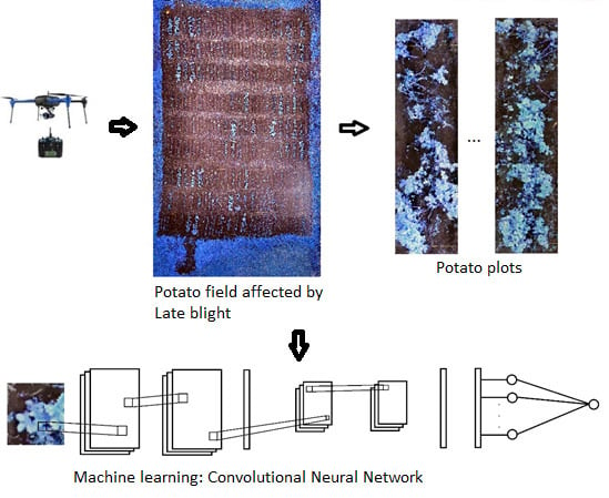
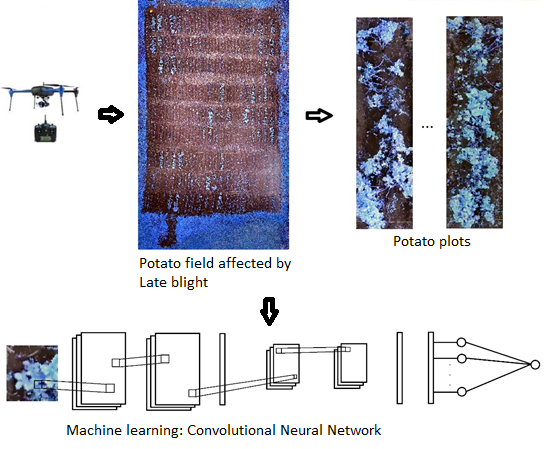
2. Materials and Methods

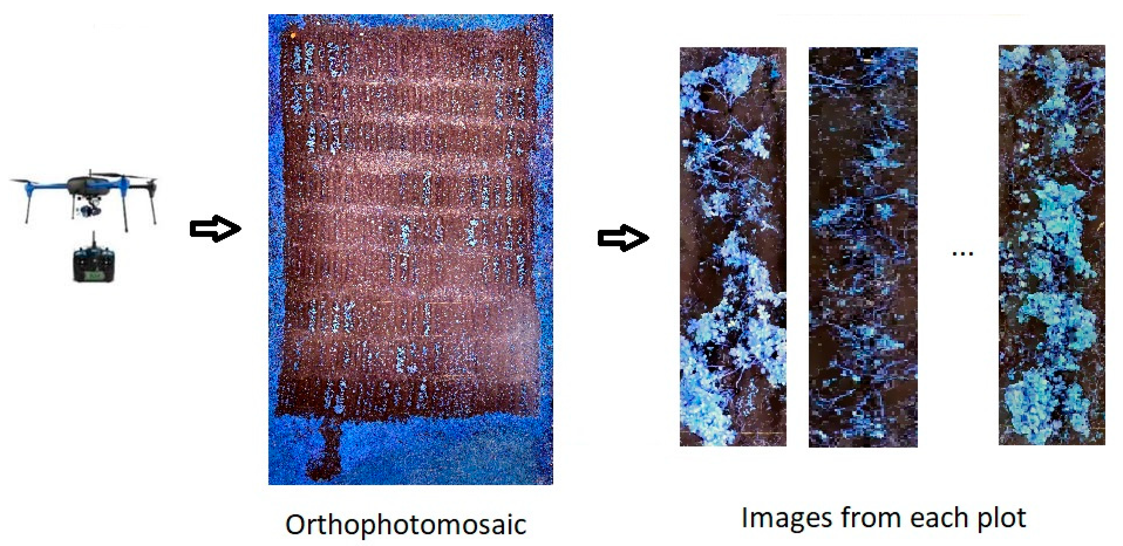
2.1. Experimental Design

In this study, 14 different potato (commercial and experimental) genotypes were planted on a farm in Ventaquemada, Boyacá-Colombia, located at 5°35′09″N, 73°52′49″W and 2780 m.a.s.l. This is a region with a high inoculum pressure of P. infestans. Three different treatments were applied to each genotype: no fungicide application, calendar fungicide application and fungicide application through integrated management (efficient, targeted application of fungicide and other preventive measures). The experiment consisted of a split-plot design with three replications, for a total of 14 × 3 × 3 = 126 different rectangular plots corresponding to 14 genotypes, 3 treatments, and 3 replications. Potato plots were spaced 1 m on each spatial direction. On each plot, 10 potato seeds were planted spaced 0.4 m. Visual evaluation of percentage of P. infestans affectation was done 40, 55, 70, and 85 days after planting, based on the disease progression [5,6].

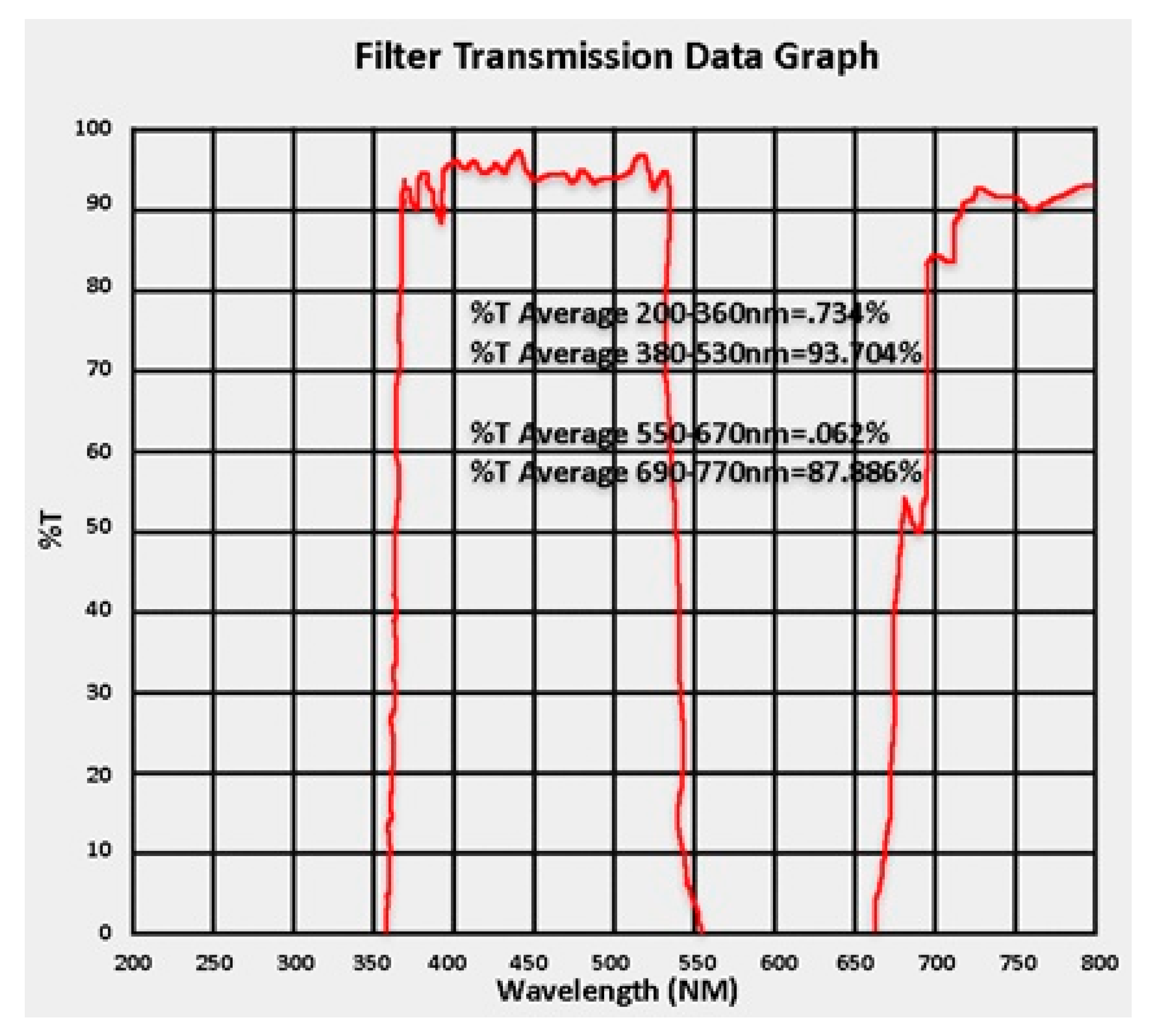
2.2. Image Acquisition and Processing

Multispectral images of the potato crop were also taken 40, 55, 70, and 85 days after planting using a low-cost 3DR IRIS+ quadcopter UAV with a Pixhawk autopilot and equipped with a GPS, flying 30 m above ground level. The IRIS+ drone was loaded with a modified Canon S110 digital camera using a blue-green-NIR filter (Figure 1) and an angle of view of 00. This kind of UAV and digital camera has been recently used for high-throughput plant phenotyping [27]. As in [27], the Canon S100 settings were TV mode, which allowed setting of a constant shutter speed. The aperture was set to be autocontrolled by the camera to maintain a good exposure level. Cannon CHDK software kit (www.chdk.wkia.com) was used to automate Canon S100’s functionality. The CHDK script allowed the UAV autopilot system to send electronic pulses to trigger the camera shutter. Spatial resolution of the images taken is 0.8 cm [27]. The raw images of Canon S100 were pre-processed using Digital Photo Professional (DPP) software developed by Canon (http://www.canon.co.uk/support/camera_software/). This software also includes lens distortion correction, chromatic aberration, and gamma correction [27].
Geometric correction of each image is performed using ground control points (GCPs) with GPS coordinates and the QGIS software (https://www.qgis.org/en/site/). Radiometric correction of each image to reflectance values is performed using the empirical line method [28] and four colored reference tarpaulins (with nominal reflectance values of 4%, 16%, 32%, and 48%), which reflectance is measured on the ground using a PS-100 apogee spectroradiometer. Before radiometric correction, dark pixel correction is performed by subtracting an image taken by the UAV with the camera shutter closed, at the end of the flight. The geometrically and radiometrically corrected images are combined to form an orthophotomosaic of the potato crop (Figure 2) using Agisoft Photoscan software (http://www.agisoft.com/). From the orthophotomosaic, rectangular images of each plot are extracted manually and saved as TIF images (see Figure 2).

2.3. Ground Truth

Expert visual evaluation of severity of P. infestans under field conditions was done at the plot level and for each of the four image acquisition campaigns. Disease severity was estimated by sampling at random four plants on each plot and computing the average percentage of the disease-infected foliar area [5,6]. Even though visual evaluation of the severity of P. infestans is susceptible to several error sources such as diseased tissue presenting no visual symptoms or the presence of other diseases also affecting foliar tissue [5], it will be considered here expert visual evaluation of late blight severity as the ground truth against which prediction performance is evaluated.

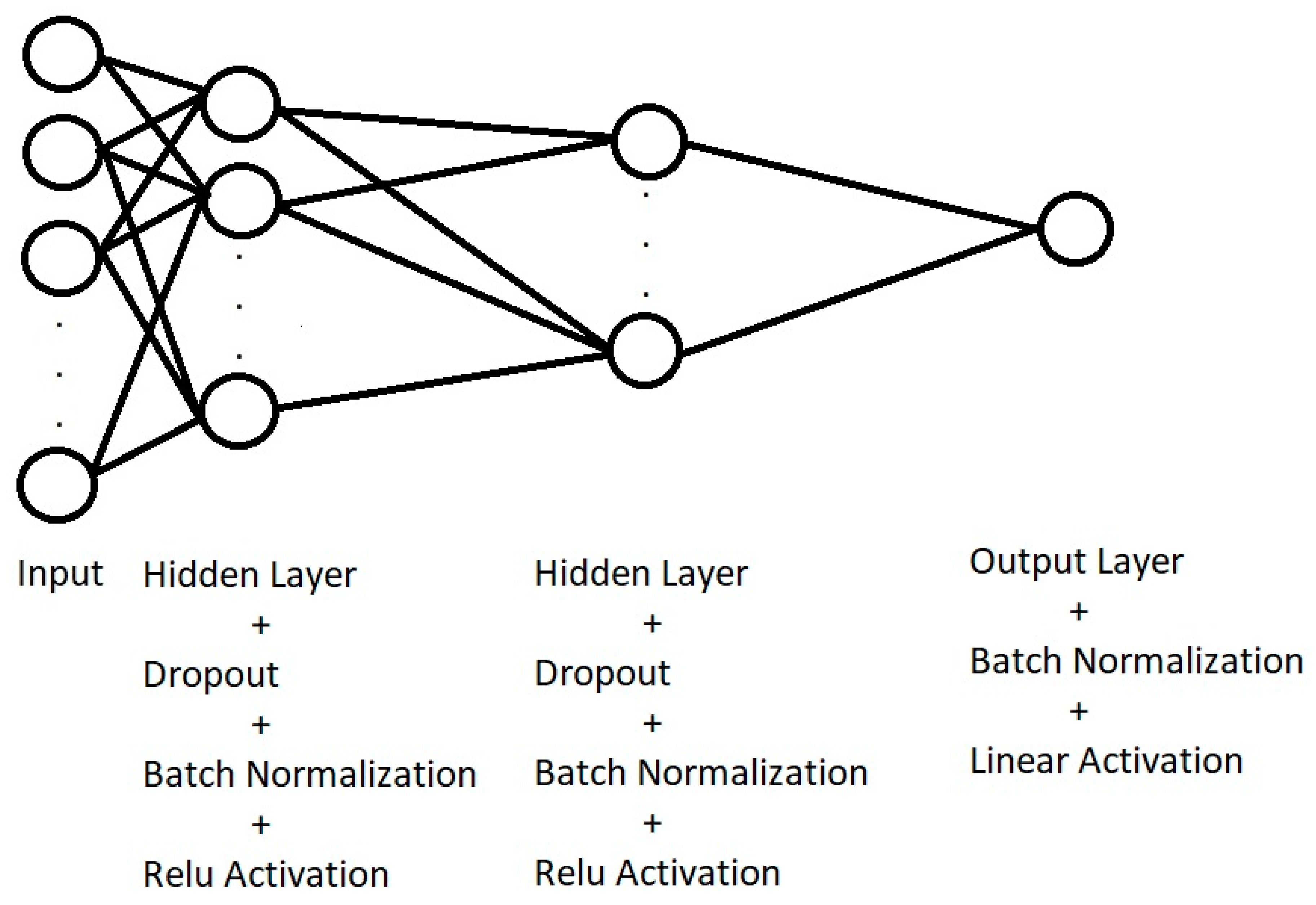
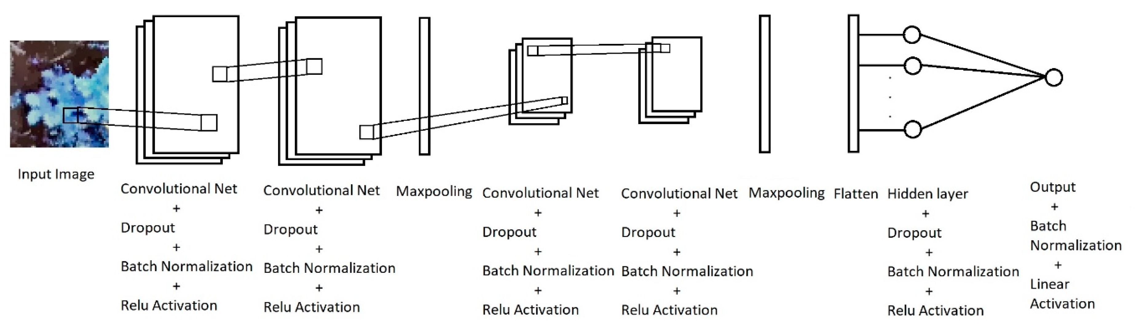
2.4. Machine Learning Algorithms

Multilayer perceptron (MLP) and convolutional neural networks (CNNs) were implemented in Python using Keras (https://keras.io/) deep learning library with Tensorflow (https://www.tensorflow.org/tutorials/) backend. Keras allows easy and fast prototyping of deep learning neural networks in Python. Support Vector Regression (SVR) and Random Forests (RFs) were implemented in Python using the Scikit-learn machine learning library (http://scikit-learn.org).
The multispectral image dataset consists of 126 images (one for each plot, see Section 2.1) acquired on each of the four image acquisition campaigns (Section 2.2) for a total of 126 × 4 = 504 rectangular multispectral images (Figure 2). Since the number of pixels of each multispectral image is relatively large (~104) and there are only 504 images, machine learning algorithms cannot be trained using the whole plot images. Instead, a sliding window of size 50 × 40 pixels is used on each plot image, moving with a step of 5 pixels along the shortest image dimension and 10 pixels along the longest image dimension. This way, a dataset consisting of 748,071 multispectral overlapping patches of size 50 × 40 pixels is obtained, thus reducing the number of multispectral pixels to be fed to the machine learning algorithms, while significantly increasing the multispectral dataset. The size of the sliding window and the steps along each axis were found as a tradeoff between increasing the image size (which allows a more complete view of the plot) and increasing the ratio of number of training images (samples)/number of features (pixels) per image, a required condition of machine learning algorithms to avoid overfitting [29]. Given that each plot was visually evaluated for late blight percentage of affectation, all the overlapping patches on each plot get assigned this ground truth, for training purposes.
The dataset is further divided into training, validation, and testing samples. The training samples are the only samples used to train the machine learning algorithms. The training and validation samples are used to select the so-called hyperparameters of the machine learning algorithms. The testing samples are used to evaluate the performance of the machine learning algorithms. Since the testing samples are not used to train or select the hyperparameters of the machine learning algorithm, they provide an estimation of how the regression algorithms would perform on unseen data. Since there are three replications of the experiment, each replication can be selected as testing dataset (~33.33% of the data) and the other two replications (~66.66% of the data) are used to extract training and validation datasets. Thirty percent of the 50 × 40 (patch) images were selected at random in two of the replications as validation samples and the remaining 70% as training samples. Since there are three replications, regression performance can be computed on each one of the replications, by using the other two replications for training and validation, as explained before, which gives us a threefold cross-validation of the performance of the machine learning algorithms used. We choose here stratified cross-validation rather than bootstrapping to evaluate performance of the machine learning algorithms implemented due to the fact that cross-validation tends to give conservative estimates of performance (upper bounds) and it is computationally much cheaper than bootstrap, which tends to give overly optimistic predictions on performance, due to the fact that in bootstrap there is a large overlap (63%) between the training and testing samples [30].
The multispectral image dataset can be better exploited by considering also spectral differences, band ratios, and dimension reduction methods such as principal components analysis (PCA). Hence, besides the multispectral dataset of (patch) images of size 50 × 40 × 3, the following additional datasets were created:
  • The spectral differences between green and blue bands and between NIR and green bands. Hence, we obtain a dataset of samples of size 50 × 40 × 2.
  • A normalized difference vegetation index (NDVI) to obtain a dataset of samples of size 50 × 40. Since we do not have separated red and NIR bands, we must use the NIR band together with either the green or blue bands to compute the NDVI. Experimentally, we found better regression performance using NDVI = (NIR − blue)/(NIR + blue).
  • The two principal components of each original multispectral plot images were extracted, and the windowing technique explained before can be used to obtain a new dataset consisting of samples of size 50 × 40 × 2. More specifically, if a plot image is of size H × W × 3, where H is the height in pixels, W the width in pixels and we have three channels, the image can be reshaped as a matrix of size P × 3 (P = H × W). Choosing the first 2 principal components, the P × 3 dataset is dimension-reduced to a P × 2 matrix, which can be reshaped as an H × W × 2 dataset, from which overlapping patches of size 50 × 40 × 2 can be extracted.
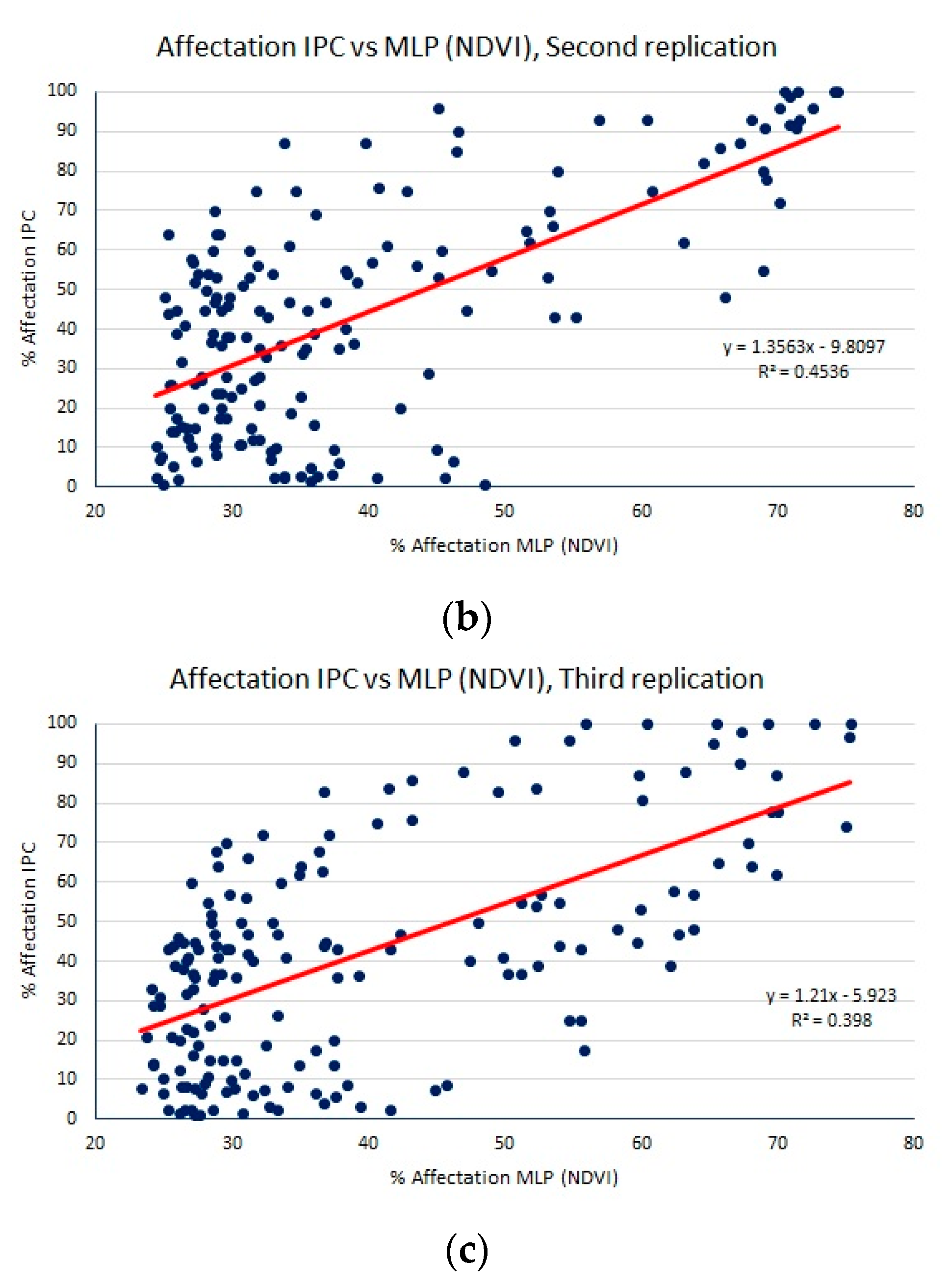
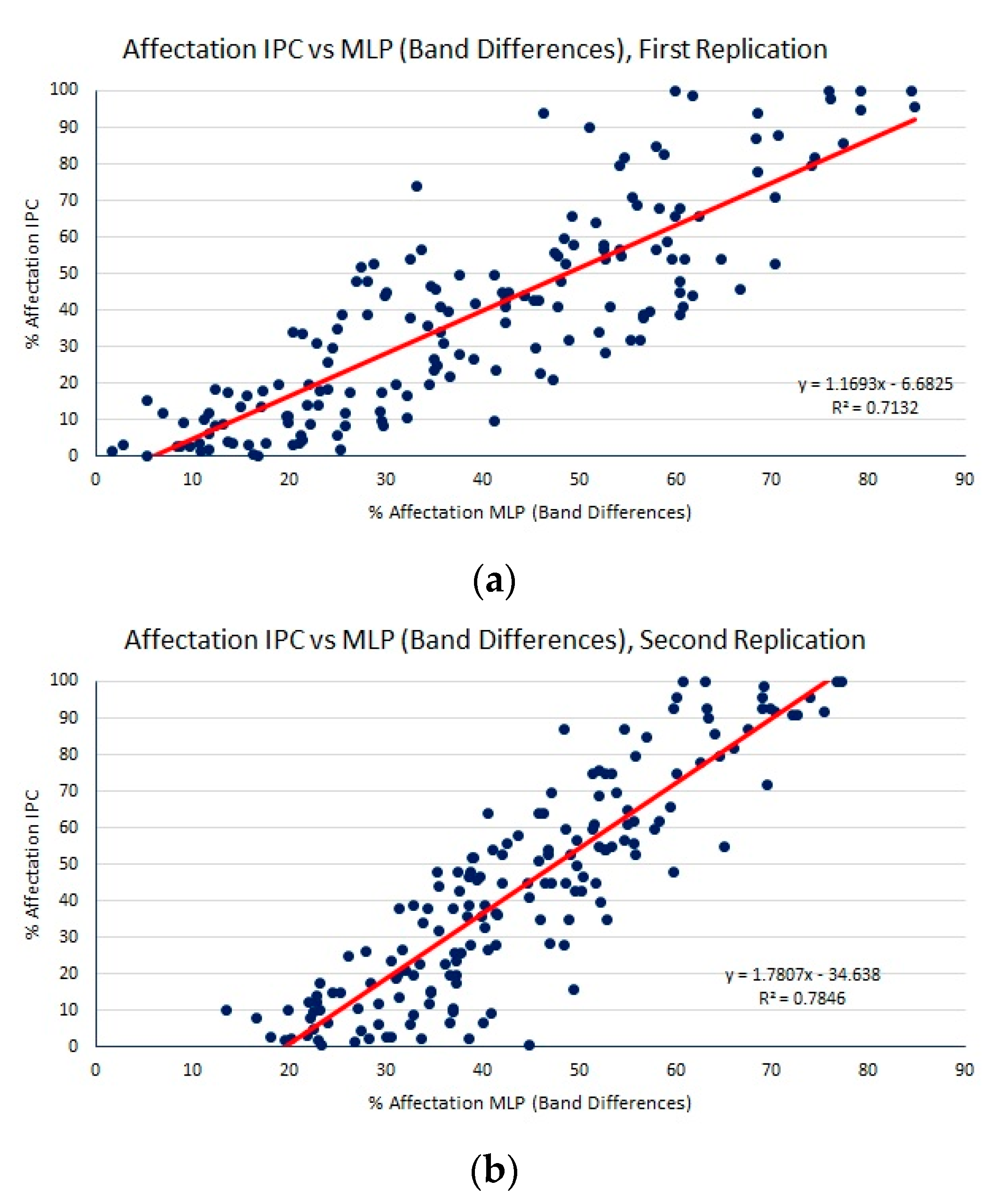
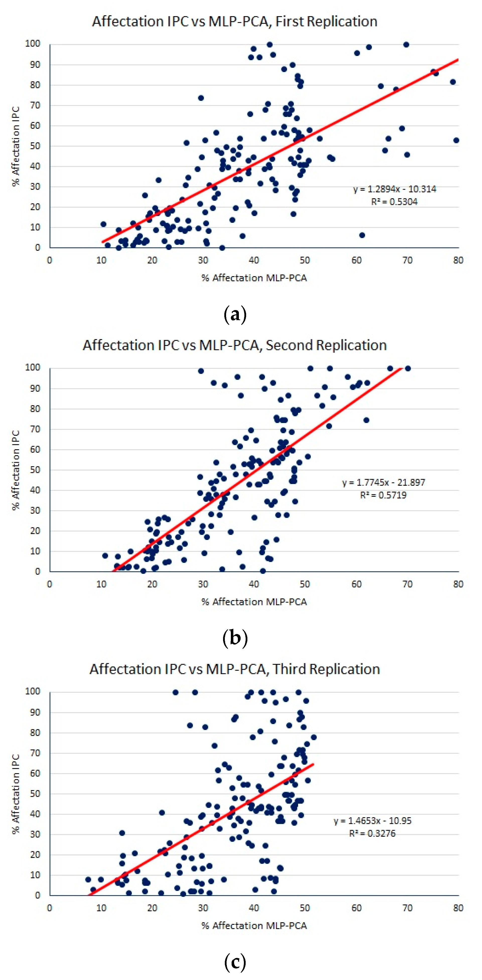
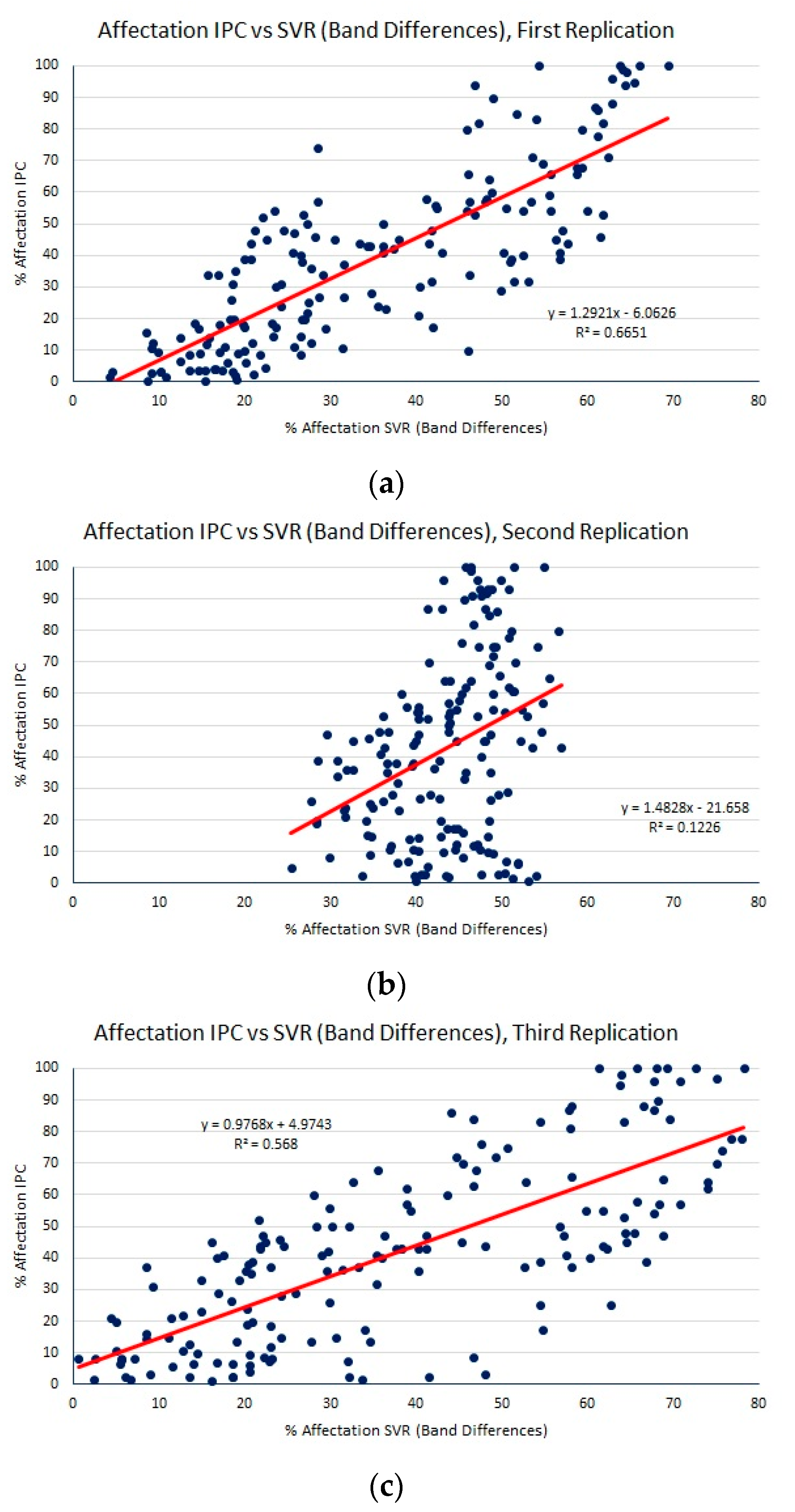
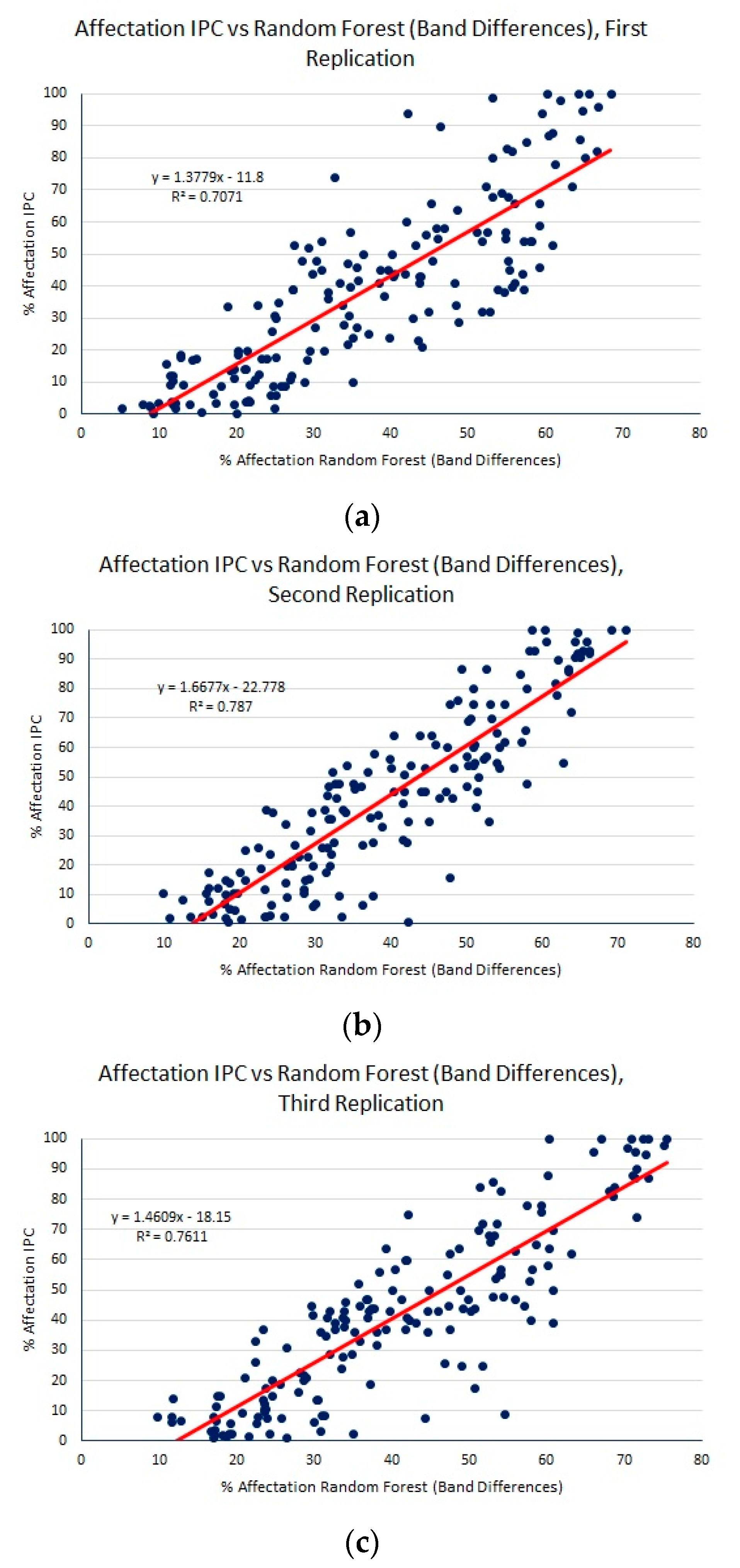
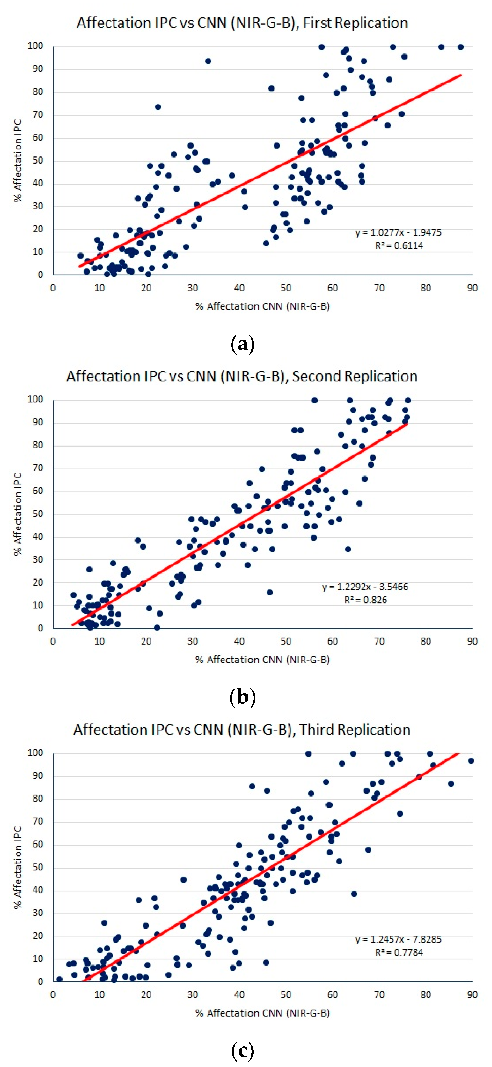
Notice that previous three datasets are not images per se. Hence, these datasets were only used to train MLP neural networks, SVR and RFs, but not to train deep learning convolutional neural networks, since convolutional neural networks use specialized filters tailored to work with images [21,26]. We use SVR and RFs only on the dataset that provided the best regression performance using MLP. Notice that all the patch images can be directly fed to the CNNs since they directly ingest images. The multiband images and datasets explained before must be reshaped as single-row vectors to be fed to the MLP, SVR, and RFs algorithms.
As mentioned before, each machine learning algorithm has several hyperparameters that need to be tuned to improve its performance, based on the training and validation datasets. In the case of MLP, the hyperparameters are: learning rate, optimization algorithm, number of epochs, number of hidden layers, and nodes on each layer. The last layer contains a single node that outputs a prediction of late blight severity, learned from the training dataset.
Good performance of MLP neural networks was found using two hidden layers containing half the nodes of the previous layer. The best learning rate found was 0.01 using Adamax optimizer, which is a variant of Adam optimizer using the infinite norm [31]. Ten epochs were enough to obtain the best validation performance (after several epochs, validation performance starts to diverge while training accuracy continues to improve, due to overfitting). Keras allows saving the best model found by checking validation performance at the end of each epoch; hence, the validation dataset was critical to avoid overfitting. Batch normalization layers [32] were added to each hidden layer. Batch normalization allows faster training (using larger learning rates), makes the network less sensitive to initialization and reduces overfitting. Dropout layers [33] were also added, with dropout probability of 0.2, to further reduce overfitting. Figure 3 summarizes the MLP architecture. Default rectified linear unit (RELU) activation layers were used, which are known to reduce training time of deep learning neural networks [21], except on the last layer, where a linear activation layer was used; in order to preserve the numerical learned output.
The same hyperparameters used on MLP were used to train convolutional neural networks, except the number of hidden layers. Since convolutional neural networks are a kind of deep learning neural network, the number of hidden layers is relatively large compared to MLP. Figure 4 shows the architecture of the convolutional neural network used. Notice that on Figure 4, 3D-like representation of CNNs layers is used, since those layers are dealing with tensor data (multispectral images and features), while MLP-like layers deal with vector data. Therefore, there is a flatten layer in CNNs that transforms tensor-valued data to vector-valued data to be processed by the fully connected MLP layers. Convolutional layers filter imaging data using feature detection kernels. Feature detection kernels of size 3 × 3 were used on the first two convolutional layers, a size typically used on the first layers to detect small features such as edges. Feature detection kernels of size 5 × 5 were used on the next two convolutional layers to detect features of larger size.
Convolutional layers also use a certain number of filters. Twenty filters were used for the first two convolutional layers and 40 filters for the last two convolutional layers. This number of filters was found using the validation dataset. The max pooling layer down samples the image features to reduce dimensionality, while summarizing information on a small window. Typical max pooling layers [26] with a window of size 2 × 2 were used.
Default hyperparameters on the support vector regression algorithm were used, except for the kernel. Best results for SVR were found using a linear kernel. Default hyperparameters for the RFs regression algorithm worked very well.

3. Results

The mean absolute error (MAE) of the predicted percentage of late blight severity was optimized for all datasets. The MAE rather than the root mean squared error (RMSE) was optimized, since it has been argued that the MAE is more adequate to evaluate mean model performance than RMSE [34,35]. Even though machine learning algorithms are trained using 50 × 40 overlapping patches, extracted from the corresponding plot images, predicting the percentage of P. infestans affectation at the plot level is the required output to be able to compare to field visual assessment. Hence, the predicted percentage of late blight severity on each testing plot (corresponding to one of the replications, not used for training or validation) is obtained by averaging the predicted percentage of affectation on all 50 × 40 overlapping patches extracted from each testing plot. The performance of MLP, SVR, RFs, and CNNs was evaluated on the four datasets mentioned before (Section 2.4), in terms of the mean absolute error (MAE), the root mean squared error (RMSE) and R-squared (R2) statistic. As indicated before, the ground truth is the percentage of P. infestans of affectation, visually estimated in the field following guidelines given by the International Potato Center (IPC) [5,6]. From now on, the ground truth will be referred to as % affectation IPC.
Figure 5, Figure 6, Figure 7 and Figure 8 compare the % affectation IPC against the % affectation predicted by MLP on the multispectral dataset with bands NIR-green-blue, the dataset using NDVI, the dataset using band differences, and the dataset using PCA decomposition; for each one of the replications.
The results shown on Figure 5, Figure 6, Figure 7 and Figure 8 indicate that the best prediction performance of MLP was achieved using band differences and the worst performance was obtained using NDVI. This could be because the NDVI relates to foliar coverage, but there is not a direct relationship between foliar coverage and the disease at early stages. Despite the best performance of MLP using band derivatives, it can be noticed that the regression line between % IPC affectation and % affectation predicted, on the second and third replications, has a large slope and intercept, resulting in higher % affectation predicted when % IPC affectation is low and lower % affectation predicted when % IPC affectation is large.
Figure 9 shows the prediction result using SVR on the band differences dataset. From these results, SVR performance in terms of MAE, RMSE, and R2 statistic is worse than the performance of MLP, especially for the second and third replications.
Figure 10 shows the performance of RFs on the band difference dataset. Notice that RFs perform better than MLP on the same dataset, for all three replications; although the slope of the regression line is relatively large.
Figure 11 shows the performance of CNNs on the NIR-G-B multispectral dataset. CNNs achieve a significant reduction in the MAE, RMSE, and R2 statistic for all three replications compared to MLP on the same data set (Figure 5). CNNs have also a low regression slope and intercept between the % affectation IPC and % affectation predicted for all three replicates. Table 1 summarizes the results of all methods in terms of cross-validation mean MAE, RMSE, and R2 statistic as well as its estimated standard error, in parenthesis. From Table 1, the best results were obtained using Random Forests and CNNs. Random Forests have the advantage of being the most stable (lower standard error) estimator, but CNNs have the lowest slope and intercept regression estimator and achieves the lowest mean MAE and RMSE, even though they did not do so well on the first replication. From these results it can be said that CNNs are better than RFs and MLP using band differences, roughly 66% of the times given the fact that it was much better than RFs and MLP using band differences for two of the three replications.

4. Discussion

In Colombia, during last year a total of 132,708 ha of potatoes were planted; late blight is currently a disease of major significance throughout the country. In the states with high potato crop production such as Cundinamarca and Boyacá, growers report 22 to 26 fungicide applications per crop season to control P. infestans, the maximum recommended by commercial brands is between 12 and 16 applications depending of the genotype and environmental conditions. On the other hand, part of the diversity of potato genetic resources (2069 accessions) are maintained in the Potato Germplasm Bank (PGB) located at the Colombian agricultural research corporation (AGROSAVIA), most of this PGB has not yet been characterized for their resistance/susceptibility to P. infestans. In this context, the development and optimization of a method for high-throughput screening of genotypes against potato late blight under field conditions is essential to identify resistant genotypes of interest for plant breeding, and to provide early warning tools for potato infected crops, supplying images that enable precise and reliable statistics.
Our results indicate that visual estimation of late blight percentage of affectation can be replaced by state-of-the-art machine learning algorithms such as CNNs, RFs, and MLP on band differences. CNNs obtained a MAE of 11.72% with a relatively small variance; which seems acceptable given the cost reduction in terms of avoiding an expert on the field going through the whole crop and the repeatability of the method. Previous work [10] reports an R2 statistic of 0.73, low errors of 4–5% and high errors of 20% for a mean RMSE of 17.1%. Hence, this work presents an improvement in terms of the R2 statistic and improvement in terms of a smaller error variance. It should be pointed out here that in this and previous work it has been assumed that the only plant stress is due to P. infestans. Hence, further work is needed to discriminate other plant stressors (biotic and abiotic) that also may affect the plant’s spectral signature and thus be confused with P. infestans.
One of the most important characteristics of late blight is that lesions and disease symptom appear quickly. Typically, green brown or yellow spots which become necrotic regions may appear in two or three days after infection with P. infestans depending on environmental conditions and potato genotype susceptibility [36]. For this reason, applicability of late blight detection using remote sensing coupled to machine learning algorithms in early warning and opportune control will depend on the capacity of this method to detect late blight symptoms at early stages. As shown in Figure 11 and Table 1, CNNs are better than RFs and MLP using band differences even when % IPC affectation is low, resulting in a higher percentage of affectation predicted, this condition could be particularly useful for an early warning system. On the other hand, at the beginning of the infection process (i.e., first 48 h) there are no visual disease symptoms; however, changes in abundance of 17,000 transcripts and 1000 secreted proteins during first hours of P. infestans infection have been reported [37]. These transcriptomic, proteomic, and metabolomic alterations can result in changes of transpiration rate, morphology, and leaf color, affecting the optical properties of the leaves. Our future research seeks to exploit the potentiality of pre-symptomatic detection. Hence, hyperspectral imaging combined with machine learning algorithms have a potential as a fast and non-invasive method to identify asymptomatic infected plants [38].
A high diversity of protectant and systemic fungicides are used by farmers to control potato late blight. In general, protectant fungicides application on potato foliage are made after 30 days of planting with additional successive applications every 7–10 days. Applications of systemic fungicides are made beginning 60 days after planting with up to 3 applications at 10 day intervals [39]. Nevertheless, it is also important to consider that late blight control should be based on an Integrated Disease Management (IDM) strategy, which in many opportunities is not the case for potato Colombian farmers. IDM is a set of strategies based on monitoring, economic thresholds, and preventive tactics to determine when disease treatment is needed [13]. Our study demonstrates the usefulness of multispectral remote sensing images to monitor late blight; multispectral imagery taken with UAVs could start after 30–40 days of planting with successive aerial images captured at 55, 70, and 85 days after planting. Remote sensing monitoring could help to optimize IDM strategy and late blight disease management decisions. Additionally, determination of percentage of P. infestans affectation using images would allow study of genotype resistance with recommendations on the use fungicides on focal points of the infection or the destruction of plots where the infection is advanced. Recently, crop protection strategies based on machine learning have been used to generate recommendations and integrated disease solutions [40]. This would avoid the indiscriminate use of fungicides and thus development of pathogen resistance.
The method presented here requires the user to manually cut images from each plot to be fed to the algorithms, this is clearly tedious and error prone. Further improvement of this technique would include a preprocessing stage where the plots are extracted from the orthophotomosaic automatically. This is not a trivial task, but CNNs have been successfully used in the past to extract objects from images [41].
Even though we have presented here state-of-the-art machine learning algorithms trained to identify percentage of P. infestans affectation, these algorithms can also be used to detect other diseases or biotic stressors. These machine learning algorithms add to the knowledge base of machine learning algorithms used for supervised crop disease detection [14,15,16].

5. Conclusions

Deep learning convolutional neural networks outperformed multilayer perceptron and support vector regression in predicting severity of P. infestans affectation on potato crops, Random Forests also performed remarkably well, followed by MLP using band differences. These results show the possibility to reliably replace visual estimation of late blight severity on potato crops using multispectral imagery taken with unmanned aerial vehicles and inexpensive digital cameras. This work also suggests the use of deep learning convolutional neural networks, Random Forests, or MLP (band differences) to detect and/or predict severity of disease in agriculture using remotely sensed multispectral images.

Author Contributions

J.D.S.-S., A.A.R., A.E.F.-R. and M.S.-S., conceived and designed the experiments. J.D.S.-S., D.F.A. and A.E.F.-R. performed the experiments. J.D.S.-S., D.F.A., A.E.F.-R., J.M.D.-C. and M.S.-S. analyzed the data. J.M.D.-C. and M.S.-S. wrote the paper. All authors read and approved the final manuscript.

Funding

This research received no external funding.

Acknowledgments

This work was supported by the Corporación colombiana de investigación agropecuaria (AGROSAVIA) and the Colombian Ministry of Agriculture and Rural Development (MADR). We thank Guillermo Sapiro (Duke University) for critically reading. We also want to thank the editor and reviewers for their accurate and helpful inputs and suggestions. We are also grateful to the Banco de Germoplasma para la Alimentación y la Agricultura de la Nación Colombiana for providing the necessary accessions used in this study from the Colombian Core Collection of potato.

Conflicts of Interest

The authors declare no conflict of interest.

References

  1. Hwang, Y.T.; Wijekoon, C.; Kalischuk, M.; Johnson, D.; Howard, R.; Prüfer, D.; Kawchuk, L. Evolution and Management of the Irish Potato Famine Pathogen Phytophthora Infestans in Canada and the United States. Am. J. Potato Res. 2014, 91, 579–593. [Google Scholar] [CrossRef]
  2. Vargas, A.M.; Ocampo, L.M.Q.; Céspedes, M.C.; Carreño, N.; González, A.; Rojas, A.; Zuluaga, A.P.; Myers, K.; Fry, W.E.; Jiménez, P.; et al. Characterization of Phytophthora infestans populations in Colombia: First report of the A2 mating type. Phytopathology 2009, 99, 82–88. [Google Scholar] [CrossRef] [PubMed]
  3. Fry, W.E. Phytophthora infestans: New Tools (and Old Ones) Lead to New Understanding and Precision Management. Annu. Rev. Phytopathol. 2016, 54, 529–547. [Google Scholar] [CrossRef] [PubMed]
  4. European and Mediterranean Plant Protection Organization. Phytophthora infestans on potato. EPPO 2008, 38, 268–271. [Google Scholar] [CrossRef]
  5. Forbes, G.; Perez, W.; Piedra, J.A. Evaluacion de la Resistencia en Genotipos de Papa a Phytophthora infestans Bajo Condiciones de Campo: Guia Para Colaboradores Internacionales; International Potato Center: Lima, Peru, 2014. [Google Scholar]
  6. Henfling, J.A. El tizón tardío de la papa: Phytophthora infestans. In Boletin de Informacion Tecnica; Instituto de Censores Jurados de Cuentas de España: Madrid, Spain, 1987; p. 25. [Google Scholar]
  7. Ray, S.S.; Jain, N.; Arora, R.K.; Chavan, S.; Panigrahy, S. Utility of Hyperspectral Data for Potato Late Blight Disease Detection. J. Indian Soc. Remote Sens. 2011, 39, 161–169. [Google Scholar] [CrossRef]
  8. Franceschini, M.H.D.; Bartholomeus, H.; van Apeldoorn, D.; Suomalainen, J.; Kooistra, L. Assessing changes in potato canopy caused by late blight in organic production systems through UAV-based pushbroom imaging spectrometer. Int. Arch. Photogramm. Remote Sens. Spat. Inf. Sci. 2017, 42, 109–112. [Google Scholar] [CrossRef]
  9. Biswas, S.; Jagyasi, B.; Singh, B.P.; Lal, M. Severity Identification of Potato Late Blight Disease from Crop Images Captured under Uncontrolled Environment. In Proceedings of the 2014 IEEE Canada International Humanitarian Technology Conference—(IHTC), Montreal, QC, Canada, 1–4 June 2014; pp. 1–5. [Google Scholar]
  10. Sugiura, R.; Tsuda, S.; Tamiya, S.; Itoh, A. ScienceDirect Field phenotyping system for the assessment of potato late blight resistance using RGB imagery from an unmanned aerial vehicle. Biosyst. Eng. 2016, 148, 1–10. [Google Scholar] [CrossRef]
  11. Liakos, K.; Busato, P.; Moshou, D.; Pearson, S.; Bochtis, D. Machine Learning in Agriculture: A Review. Sensors 2018, 18, 2674. [Google Scholar] [CrossRef] [PubMed]
  12. Balducci, F.; Impedovo, D.; Pirlo, G. Machine Learning Applications on Agricultural Datasets for Smart Farm Enhancement. Machines 2018, 6, 38. [Google Scholar] [CrossRef]
  13. Durgabai, R.P.L.; Bhargavi, P. Pest Management using Machine Learning Algorithms: A Review. Int. J. Comput. Sci. Eng. Inf. Technol. Res. 2018, 8, 13–22. [Google Scholar]
  14. Corrales, D.C. Toward detecting crop diseases and pest by supervised learning. Ing. Univ. 2015, 19, 207–228. [Google Scholar] [CrossRef]
  15. Revathi, P.; Revathi, R.; Hemalatha, M. Comparative Study of Knowledge in Crop Diseases Using Machine Learning Techniques. Int. J. Comput. Sci. Inf. Technol. 2011, 2, 2180–2182. [Google Scholar]
  16. Tripathi, M.K.; Maktedar, D.D. Recent machine learning based approaches for disease detection and classification of agricultural products. In Proceedings of the 2016 International Conference on Computing Communication Control and automation (ICCUBEA), Pune, India, 12–13 August 2016; pp. 1–6. [Google Scholar]
  17. Alves, D.P.; Tomaz, R.S.; Laurindo, B.S.; Laurindo, R.D.F.; Cruz, C.D.; Nick, C.; Silva, D.J.H.D. Artificial neural network for prediction of the area under the disease progress curve of tomato late blight. Sci. Agric. 2017, 74, 51–59. [Google Scholar] [CrossRef] [Green Version]
  18. Moshou, D.; Bravo, C.; West, J.; Wahlen, S.; McCartney, A.; Ramon, H. Automatic detection of ‘yellow rust’ in wheat using reflectance measurements and neural networks. Comput. Electron. Agric. 2004, 44, 173–188. [Google Scholar] [CrossRef]
  19. Wang, X.; Zhang, M.; Zhu, J.; Geng, S. Spectral prediction of Phytophthora infestans infection on tomatoes using artificial neural network (ANN). Int. J. Remote Sens. 2008, 29, 1693–1706. [Google Scholar] [CrossRef]
  20. Wasserman, P.D.; Schwartz, T. Neural networks. II. What are they and why is everybody so interested in them now? IEEE Expert 1988, 3, 10–15. [Google Scholar] [CrossRef]
  21. Krizhevsky, A.; Sutskever, I.; Hinton, G.E. ImageNet Classification with Deep Convolutional Neural Networks. Adv. Neural Inf. Process. Syst. 2012, 1097–1105. [Google Scholar] [CrossRef]
  22. Firdaus, P.; Arkeman, Y.; Buono, A.; Hermadi, I. Satellite image processing for precision agriculture and agroindustry using convolutional neural network and genetic algorithm. In IOP Earth and Environmental Science; IOP Publishing: Bristol, UK, 2017; p. 7. [Google Scholar]
  23. Sladojevic, S.; Arsenovic, M.; Anderla, A.; Culibrk, D.; Stefanovic, D. Deep Neural Networks Based Recognition of Plant Diseases by Leaf Image Classification. Comput. Intell. Neurosci. 2016, 2016, 11. [Google Scholar] [CrossRef] [PubMed]
  24. Smola, A.J.; Sch, B.; Schölkopf, B. A Tutorial on Support Vector Regression. Stat. Comput. 2004, 14, 199–222. [Google Scholar] [CrossRef]
  25. Ho, T.K. Random decision forests. In Proceedings of the IEEE Third International Conference on Document Analysis and Recognition, Montreal, QC, Canada, 14–16 August 1995; pp. 278–282. [Google Scholar]
  26. O’Shea, K.; Nash, R. An Introduction to Convolutional Neural Networks. 2015. Available online: https://arxiv.org/pdf/1511.08458.pdf (accessed on 7 July 2018).
  27. Haghighattalab, A.; Pérez, L.G.; Mondal, S.; Singh, D.; Schinstock, D.; Rutkoski, J.; Ortiz-Monasterio, I.; Singh, R.P.; Goodin, D.; Poland, J. Application of unmanned aerial systems for high throughput phenotyping of large wheat breeding nurseries. Plant. Methods 2016, 12, 35. [Google Scholar] [CrossRef] [PubMed]
  28. Smith, G.M.; Milton, E.J. The use of the empirical line method to calibrate remotely sensed data to reflectance. Int. J. Remote Sens. 1999, 20, 2653–2662. [Google Scholar] [CrossRef]
  29. Raudys, S.; Jain, A. Small sample size effects in statistical pattern recognition: Recommendations for practitioners. IEEE Trans. Pattern Anal. Mach. Intell. 1991, 13, 252–264. [Google Scholar] [CrossRef]
  30. Kohavi, R. A Study of Cross-Validation and Bootstrap for Accuracy Estimation and Model Selection A Study of Cross-Validation and Bootstrap for Accuracy Estimation and Model Selection. In Proceedings of the 14th International Joint Conference on Artificial Intelligence, Montreal, QC, Canada, 20–25 August 1995; pp. 1137–1143. [Google Scholar]
  31. Kingma, D.P.; Ba, J. Adam: A Method for Stochastic Optimization. In Proceedings of the 3rd International Conference on Learning Representations, Banff, AB, Canada, 14–16 April 2014; pp. 1–15. [Google Scholar]
  32. Ioffe, S.; Szegedy, C. Batch Normalization: Accelerating Deep Network Training by Reducing Internal Covariate Shift. In Proceedings of the 32nd International Conference on Machine Learning, Lille, France, 6–11 July 2015; pp. 81–87. [Google Scholar]
  33. Srivastava, N.; Hinton, G.; Krizhevsky, A.; Sutskever, I.; Salakhutdinov, R. Dropout: A Simple Way to Prevent Neural Networks from Overfitting. J. Mach. Learn. Res. 2014, 15, 1929–1958. [Google Scholar]
  34. Willmott, C.J.; Matsuura, K. Advantages of the mean absolute error (MAE) over the root mean square error (RMSE) in assessing average model performance. Clim. Res. 2005, 30, 79–82. [Google Scholar] [CrossRef] [Green Version]
  35. Willmott, C.J.; Matsuura, K.; Robeson, S.M. Ambiguities inherent in sums-of-squares-based error statistics. Atmos. Environ. 2009, 43, 749–752. [Google Scholar] [CrossRef]
  36. Fry, W.E. Phytophthora infestans: The plant (and R gene) destroyer. Mol. Plant. Pathol. 2008, 9, 385–402. [Google Scholar] [CrossRef] [PubMed]
  37. Ali, A.; Alexandersson, E.; Sandin, M.; Resjö, S.; Lenman, M.; Hedley, P.; Levander, F.; Andreasson, E. Quantitative proteomics and transcriptomics of potato in response to Phytophthora infestans in compatible and incompatible interactions. BMC Genom. 2014, 15, 497. [Google Scholar] [CrossRef] [PubMed]
  38. Zhu, H.; Chu, B.; Zhang, C.; Liu, F.; Jiang, L.; He, Y. Hyperspectral Imaging for Presymptomatic Detection of Tobacco Disease with Successive Projections Algorithm and Machine-learning Classifiers. Sci. Rep. 2017, 7, 4125. [Google Scholar] [CrossRef] [PubMed]
  39. Majeed, A.; Muhammad, Z.; Ullah, Z.; Ullah, R.; Ahmad, H. Late Blight of Potato (Phytophthora infestans) I: Fungicides Application and Associated Challenges. Turk. J. Agric. Food Sci. Technol. 2017, 5, 261–266. [Google Scholar] [CrossRef]
  40. Van Evert, F.K.; Fountas, S.; Jakovetic, D.; Crnojevic, V.; Travlos, I.; Kempenaar, C. Big Data for weed control and crop protection. Weed Res. 2017, 57, 218–233. [Google Scholar] [CrossRef] [Green Version]
  41. Szegedy, C. Deep Neural Networks for Object Detection. In Advances in Neural Information Processing Systems; The MIT Press: Cambridge, MA, USA, 2013; pp. 2553–2561. [Google Scholar]
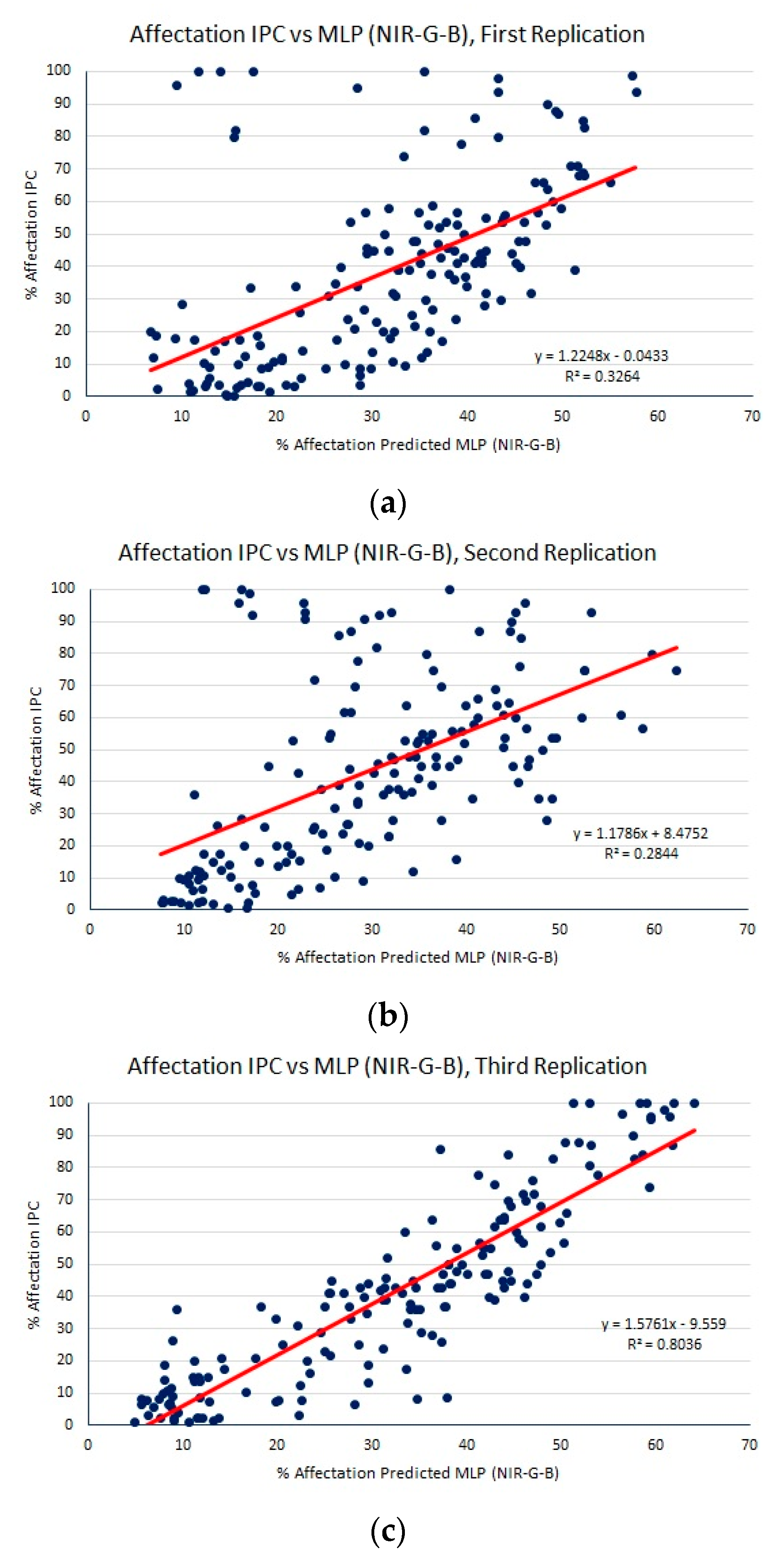
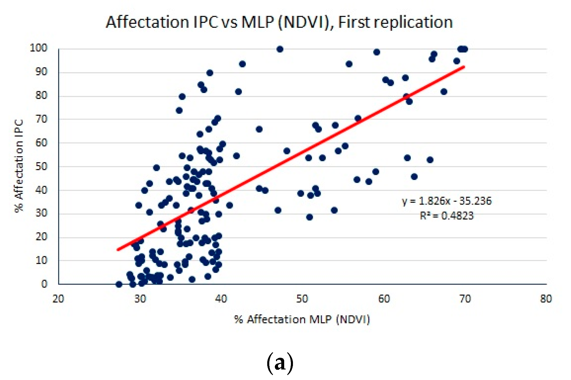
Figure 1. Transmission bands of the camera filter.
Remotesensing 10 01513 g001
Figure 2. Image acquisition methodology. (Left): drone, Center: orthophotomosaic, (Right): plot images.
Remotesensing 10 01513 g002
Figure 3. Multilayer Perceptron architecture.
Remotesensing 10 01513 g003
Figure 4. Convolutional neural network architecture indicating in detail each one of the convolutional and hidden layers.
Remotesensing 10 01513 g004
Figure 5. Percentage of P. infestans affectation using IPC methodology vs. estimated percentage of affectation using MLP on the NIR-G-B multispectral dataset, for (a) first replication, MAE: 16.50, RMSE: 23.74, R2: 0.3264; (b) second replication, MAE: 19.00, RMSE: 28.03, R2: 0.2844; (c) third replication, MAE: 13.63, RMSE: 18.00, R2: 0.8036. IPC: International Potato Center; MLP: Multilayer Perceptron; NIR: near infrared; MAE: mean absolute error; RMSE: root mean squared error.
Remotesensing 10 01513 g005
Figure 6. Percentage of P. infestans affectation using IPC methodology vs. estimated percentage of affectation using MLP on the NDVI dataset, for (a) first replication, MAE: 18.48, RMSE: 21.58, R2: 0.4823; (b) second replication, MAE: 18.84, RMSE: 22.24, R2: 0.4536; (c) third replication, MAE: 18.79, RMSE: 22.12, R2: 0.398. NDVI: Normalized Difference Vegetation index.
Remotesensing 10 01513 g006aRemotesensing 10 01513 g006b
Figure 7. Percentage of P. infestans affectation using IPC methodology vs. estimated percentage of affectation using MLP on the band differences dataset, for (a) first replication, MAE: 12.03, RMSE: 15.05, R2: 0.7132; (b) second replication, MAE: 14.44, RMSE: 17.43, R2: 0.7846; (c) third replication, MAE: 13.21, RMSE: 16.38, R2: 0.7416.
Remotesensing 10 01513 g007aRemotesensing 10 01513 g007b
Figure 8. Percentage of P. infestans affectation using IPC methodology vs. estimated percentage of affectation using MLP on the PCA dataset, for (a) first replication, MAE: 15.06, RMSE: 19.31, R2: 0.5304; (b) second replication, MAE: 16.95, RMSE: 22.03, R2: 0.5719; (c) third replication, MAE: 17.80, RMSE: 24.28, R2: 0.3276. PCA: principal components analysis.
Remotesensing 10 01513 g008
Figure 9. Percentage of P. infestans affectation using IPC methodology vs. estimated percentage of affectation using SVR on the band differences dataset for (a) first replication, MAE: 13.84, RMSE: 17.12, R2: 0.6651; (b) second replication, MAE: 22.45, RMSE: 27.16, R2: 0.1226; (c) third replication, MAE: 15.75, RMSE: 18.91, R2: 0.568. SVR: support vector regression.
Remotesensing 10 01513 g009
Figure 10. Percentage of P. infestans affectation using IPC methodology vs. estimated percentage of affectation using RFs on the band differences dataset, for (a) first replication, MAE: 13.04, RMSE: 15.98, R2: 0.7071; (b) second replication, MAE: 12.81, RMSE: 16.16, R2: 0.7870; (c) third replication, MAE: 13.02, RMSE: 16.31, R2: 0.7611. RF: Random Forests.
Remotesensing 10 01513 g010
Figure 11. Percentage of P. infestans affectation using IPC methodology vs. estimated percentage of affectation using CNNs on the NIR-G-B multispectral dataset, for (a) first replication, MAE: 13.56, RMSE: 17.10, R2: 0.6114; (b) second replication, MAE: 10.83, RMSE: 13.93, R2: 0.8260; (c) third replication, MAE: 10.83, RMSE: 13.93, R2: 0.8260. CNN: convolutional neural networks.
Remotesensing 10 01513 g011
Table 1. Summary of Regression Results.
Regression MethodMAERMSER2
MLP (NIR-G-B)16.37 (1.55)23.25 (2.90)0.47 (0.17)
MLP (NDVI)18.71 (0.11)21.98 (0.20)0.44 (0.02)
MLP (band differences)13.23 (0.70)16.28 (0.70)0.75 (0.02)
MLP (PCA)16.60 (0.81)21.87 (1.44)0.48 (0.08)
SVR (band differences)17.34 (2.61)21.06 (3.09)0.45 (0.17)
RFs (band differences)12.96 (0.07)16.15 (0.07)0.75 (0.02)
CNNs (NIR-G-B)11.72 (0.92)15.09 (1.01)0.74 (0.07)

