End-to-End Airport Detection in Remote Sensing Images Combining Cascade Region Proposal Networks and Multi-Threshold Detection Networks

Abstract

Fast and accurate airport detection in remote sensing images is important for many military and civilian applications. However, traditional airport detection methods have low detection rates, high false alarm rates and slow speeds. Due to the power convolutional neural networks in object-detection systems, an end-to-end airport detection method based on convolutional neural networks is proposed in this study. First, based on the common low-level visual features of natural images and airport remote sensing images, region-based convolutional neural networks are chosen to conduct transfer learning for airport images using a limited amount of data. Second, to further improve the detection rate and reduce the false alarm rate, the concepts of “divide and conquer” and “integral loss’’ are introduced to establish cascade region proposal networks and multi-threshold detection networks, respectively. Third, hard example mining is used to improve the object discrimination ability and the training efficiency of the network during sample training. Additionally, a cross-optimization strategy is employed to achieve convolution layer sharing between the cascade region proposal networks and the subsequent multi-threshold detection networks, and this approach significantly decreases the detection time. The results show that the method established in this study can accurately detect various types of airports in complex backgrounds with a higher detection rate, lower false alarm rate, and shorter detection time than existing airport detection methods.

1. Introduction

Object detection based on remote sensing images is currently a research topic of interest in the field of image processing. As military and civilian infrastructures, airports play important roles in various processes, such as aircraft transportation and energy supply. However, because airports have complex backgrounds and varying shapes and sizes, accurate and real-time airport detection remains problematic and challenging.

Deep learning has become a leading research topic in industry and academia. Zhu et al. [1] proposed that deep learning has been rapidly developed in image analysis tasks, including image indexing, segmentation, and object classification and detection. At the same time, deep learning also promotes the development of remote sensing image analysis. Object detection is an important task in remote sensing image analysis. Compared with traditional classifiers based on manually designed features, convolutional neural networks have better representation characteristics of abstract features. Therefore, more and more scholars have begun to study object detection based on convolutional neural networks in remote sensing images, such as vehicle detection [2,3], oil tank detection [4], aircraft detection [5], and ship detection [6]. To date, a variety of airport detection methods have been proposed, and they can be divided into two categories: edge-based detection [7,8,9,10,11,12] and detection based on region segmentation [13,14]. Edge-based detection focuses on the characteristics of the lines at edges, and achieves airport detection through the detection of runways. This approach is fast and simple but susceptible to interference from non-airport objects with long straight-line features. Airport detection based on region segmentation focuses on the distinct structural features of airports, but such methods have significant efficiency issues that are difficult to overcome due to the problem of overlapping sliding windows. In summary, the major problems and shortcomings of the aforementioned methods are as follows. The sliding window strategy lacks objected detection, and it has high temporal complexity and window redundancy. Additionally, the manually designed features of this method are not sufficiently robust to account for variations derived from airport diversity.

In recent years, deep learning has provided new methods of airport detection. The transfer learning ability of convolutional neural networks (CNNs) has been used to recognize airport runways and airports [15,16]. CNNs have also been used to extract multi-scale deep fusion features from images that were then classified using support vector machine methods [17]. However, these methods mainly use only the powerful feature extraction or classification capabilities of the associated CNNs, and the region proposal methods are based on manual methods such as edge or region segmentation, in which the limitations of traditional methods remain. In 2014, Girshick et al. [18] proposed region-based convolutional neural networks (R-CNNs), which made breakthroughs in object detection and considerably improved object detection based on deep learning. Girshick [19] proposed a region of interest (RoI) pooling layer to extract a fixed-length feature vector from the feature map at a single scale. To further improve the accuracy and speed of R-CNNs, Ren et al. [20] later proposed Faster R-CNNs, a successor to R-CNNs, which uses region proposal networks (RPNs) to replace the selective search (SS) algorithm [21] as the region proposal method. This approach enables the sharing of convolutional layers between the RPNs and the subsequent detection networks, which significantly improves the speed of the algorithm. The training of a deep learning model requires a large amount of sample data, but the number of airport remote sensing images is insufficient for training a network model. However, the large number of successful applications of transfer learning theory [22] in object recognition and detection tasks represents a potential direction for solving the problem of inadequate airport data.

Thus, in this study, using an end-to-end Faster R-CNN as the basic framework and based on the establishment of a remote sensing image database, we perform transfer learning with pretraining models, improve and optimize the network model and ultimately achieve fast and accurate airport detection.

The main contributions of this study are as follows.

A fast and accurate detection model is developed for airport detection based on remote sensing images. Unlike the conventional methods that involve a sliding window with manual operations and simply use a CNN as the classification tool, the method developed in this study integrates object detection in a deep network framework that enables the sharing of the convolution layer between the front-end cascade RPNs and the subsequent multi-threshold detection networks, and this method features an entire end-to-end framework.

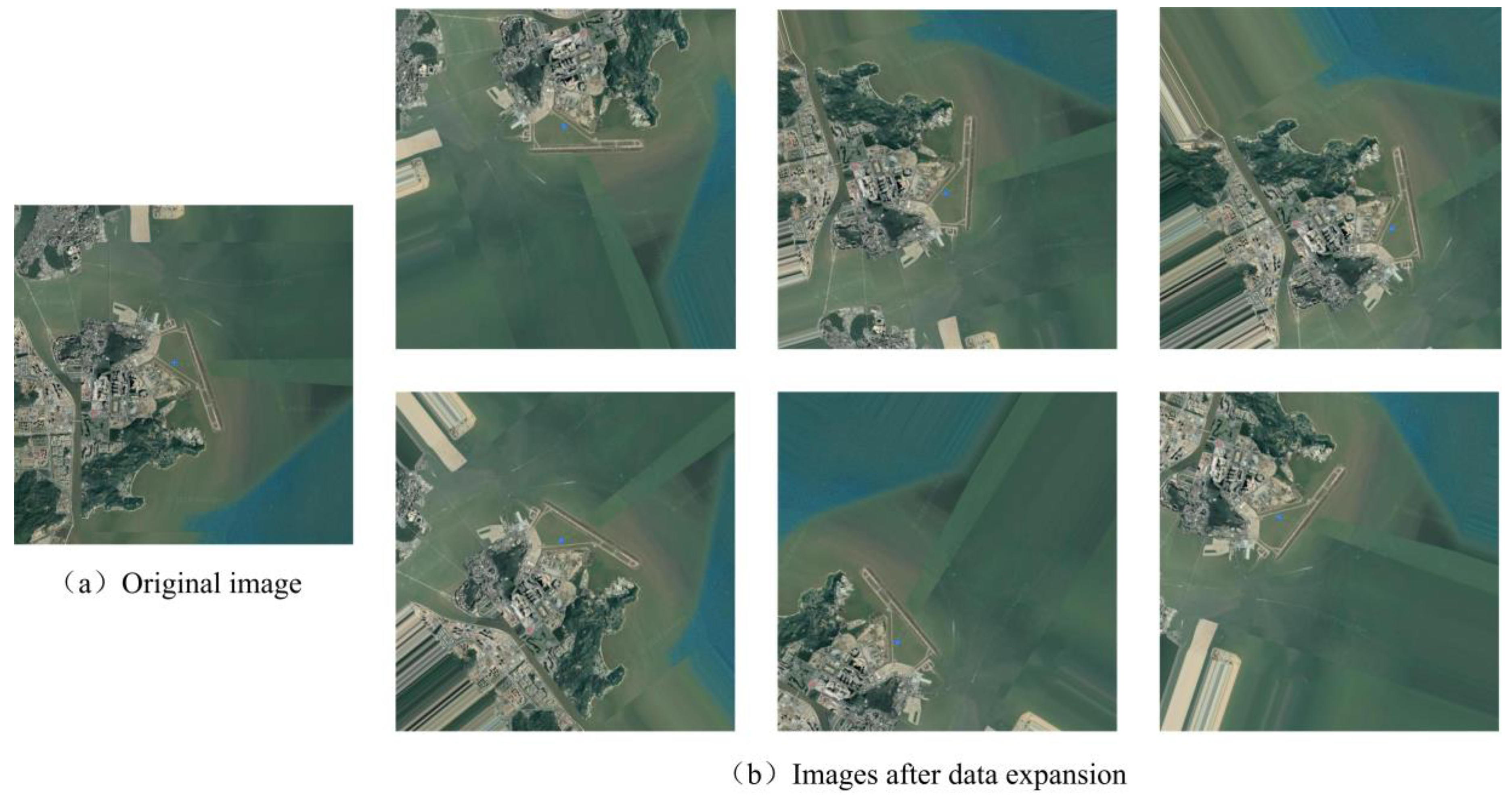
A remote sensing image database is established, and the amount of data is artificially increased using a data expansion technique to prevent the overfitting of the training model. This approach provides the foundation for subsequent applications of the deep learning model in the field of airport detection.

The concept of “divide and conquer” is introduced to improve the RPN and establish the network structure by proposing a cascade region. This technique is simple to implement and has a very small additional computational cost; moreover, it can enhance airport detection performance by improving the quality of the candidate boxes.

The loss function of the detection networks indiscriminately processes the detection boxes that have an intersection over union (IoU) greater than the threshold, which leads to poor positioning accuracy; thus, multiple IoU training thresholds are introduced to improve the loss function and the accuracy of airport detection.

Hard example mining is employed to use hard examples in model training to improve the object discriminative ability and training effectiveness of the networks. This method yields optimal performance for the network model.

2. Materials and Methods

We first introduce the network architecture of Faster R-CNN, and then present some specific improvement of the proposed method. The flowchart of the proposed algorithm is shown in Figure 1.

2.1. Related Work

The overall structure of the Faster R-CNN is shown in Figure 2, in which one image is used as the input, and the prediction probability value and object detection box of the object category are used as the output. This method mainly involves RPNs and detection networks, which include RoI pooling layers, fully connected layers, and classification and regression layers. Because the two networks share the convolutional layer, which enables object detection to be unified in a deep network framework, the entire network framework has end-to-end characteristics.

2.1.1. Region Proposal Networks

After the convolutional feature map processed by the RPNs [20] is outputted by the shared convolutional layer, the rectangle candidate box sets, as shown in Figure 3, are generated. RPNs uses a sliding window that is 3 × 3 in size to perform the convolutional operation on the feature map, in which each sliding window is mapped to a lower-dimensional vector. After the convolutional operation using the 1 × 1 convolution kernel, the results are outputted to classification layers and regression layers to simultaneously conduct object classification and position regression for the candidate boxes. Notably, the classification process determines the presence or absence of a discriminative object rather than a specific category, and position regression refers to the translation scaling parameter of the candidate box.

To accommodate multi-scale objects, candidate boxes with multiple sizes and aspect ratios at each location on the convolutional feature map are considered. The parametric representation of a candidate box is called an anchor, and each anchor corresponds to a set of sizes and aspect ratios. For each sliding window, three sizes (128², 256², and 512² pixels) and three aspect ratios (1:1, 1:2, and 2:1)—i.e., 9 types of anchors—are considered to address the multi-scale objects in the image. For the positioning accuracy of the bounding box, employ the IoU formula. The IoU indicates the degree of overlap between bounding box A and the ground truth B, as shown in the Equation (1). The larger the IoU, the more accurate the positioning of bounding box A.

$$\mathrm{IoU}=\left(A\cap B\right)/\left(A\cup B\right)$$

(1)

To train the RPNs, each anchor is assigned a binary tag. A positive tag (object) is assigned to two types of anchors: the anchor that has the highest IoU for a certain “ground truth” box, and anchors that have an IoU greater than 0.7 for any manually tagged box. A negative tag (non-object) is assigned to any anchor that has an IoU lower than 0.3 for all the manually tagged boxes. Based on the multi-task loss principle [12], the two tasks—object classification and candidate box regression—are simultaneously completed and, thus, the loss function of the RPNs is defined as follows:

$$L\left(\{p_i\},\{t_i\}\right)=\raisebox{1ex}{$1$}\!\left/ \!\raisebox{-1ex}{$N_{cls}$}\right.{\displaystyle \sum _i{L}_{cls}}\left(p_i,p_i{}^{*}\right)+\raisebox{1ex}{$\lambda $}\!\left/ \!\raisebox{-1ex}{$N_{reg}$}\right.{\displaystyle \sum _i{p}_i{}^{*}{L}_{reg}}\left(t_i,t_i{}^{*}\right)$$

(2)

where $i$ is the index of the anchor in a small batch of samples and $p_i$ is the prediction probability of the event that the $i$ anchor contains the object. If the true tag of the anchor is positive, then $p_i{}^{*}=1$. If the true tag of the anchor is negative, then $p_i{}^{*}=0$. Here, $t_i$ represents the parameterized coordinates of the candidate box, and $t_i{}^{*}$ represents the coordinates of the manually tagged box. $N_{cls}$ and $N_{reg}$ are normalization constants that represent the number of samples in the small batch and number of anchors, respectively. Here, $\lambda$ is an adjustable equilibrium weight, and $L_{cls}$ and $L_{reg}$ are classification and regression losses, respectively, which are defined as follows:

$$L_{cls}\left(x,y\right)=-log{x}_y$$

(3)

$$L_{reg}(t_i,t_i^{*})=\{\begin{array}{l}0.5{\left(t_i-t_i^{*}\right)}^2\hspace{0.17em}\hspace{0.17em}\hspace{0.17em}\hspace{0.17em}\hspace{0.17em}\hspace{0.17em}if\left|t_i-t_i^{*}\right|<1\\ \left|t_i-t_i^{*}\right|-0.5\hspace{0.17em}\hspace{0.17em}\hspace{0.17em}\hspace{0.17em}\hspace{0.17em}\hspace{0.17em}\hspace{0.17em}\hspace{0.17em}otherwise\end{array}$$

(4)

2.1.2. Non-Maximum Suppression

In the candidate boxes generated by the RPNs, multiple candidate boxes could surround the same object and overlap in large numbers. Therefore, based on the object classification score of the candidate box, Non-maximum suppression (NMS) is used to eliminate candidate boxes with a low score and reduce redundancy. Essentially, NMS is an iteration-traversal-elimination process in which the number of candidate boxes can be drastically reduced through setting the IoU threshold without affecting the accuracy of airport detection.

2.1.3. Region of Interest Pooling Layer

Many incidences of overlap among thousands of candidate regions (the region within a candidate box) can be present and result in a high time cost for feature extraction. Because of the existence of a certain mapping relationship between the candidate region feature map and the complete feature map, feature extraction can be first performed on the entire image and, then, the corresponding RoI feature vector of the candidate region is mapped directly without repetitively extracting features, thereby reducing the time cost of the model. Mini-batch sample training is used for the convolutional operations of the shared candidate regions. For each mini-batch, $B$, $N$ candidate regions are sampled; i.e., a total of $B/N$ candidate regions are used from the same image and share the convolutional operations.

2.2. The Proposed Method

2.2.1. Transfer Learning

For each of the object tasks, traditional machine learning algorithms must be retrained, but transfer learning can learn the common features of multiple tasks and apply them to new object tasks [22]. The lower convolutional layers in the CNNs only learn low-level semantic features, such as edges and colors, which are identical in airport images and normal natural images, as shown in Figure 4. The higher convolutional layers extract more complex and abstract features, such as shapes and other combined features, and the final convolutional layers and fully connected layers play decisive roles in various tasks. Therefore, in new airport detection tasks, the parameters of the lower convolutional layers in the pretraining model remain unchanged or are iterated at a small learning rate to ensure that the common features previously learned can be transferred to a new task. In this study, the pretraining network VGG16 [23] in ImageNet [24], a large-scale recognition database, is used to initialize the weight parameters of the shared convolution layers. Then, the airport database is used to perform fine-tuned training. The result shows that transfer learning using the initial values of VGG16 is very effective.

2.2.2. Cascade Region Proposal Networks

The ideal region proposal method is to generate as few candidate boxes as possible but to cover every target in the image, while a large number of background regions still exist in the airport candidate boxes generated by the RPNs. The performance can be enhanced by reducing the number of candidate boxes generated by clustering [25], and the quality of the candidate boxes can be improved by reordering the candidate boxes via the CNNs [26]. These methods inspired us to adopt the strategy of “divide and conquer” to improve the RPNs, and we propose the cascade RPNs structure shown in Figure 5.

Two standard RPNs are connected in tandem, of which the first generates candidate boxes using the correspondence between the sliding window and the anchor, and the second generates candidate boxes using the correspondence between the input candidate boxes and the anchors on the feature map. Based on the classification score of each candidate box, NMS is used after each RPN to further reduce redundancy. To match the network model with the airport detection task, the dimension and aspect ratio of the anchors in the RPNs are set based on the airport size and shape features in the dataset and experimental verification, as shown in

Table 1. Parameter values.

	Size (Pixels)	Aspect Ratio
Value	(1282, 1922, 2562)	(1:1, 2:3, 3:2)

.

2.2.3. Multi-Threshold Detection Networks

The RoI feature vector is exported to the fully connected layer and ultimately outputted from two peer output layers. One outputs the prediction probability of the background and the object from the $K$ category, and the other outputs the regression value of the detection box of the object from the $K$ category $t^k=\left(t_x^k,t_y^k,t_w^k,t_h^k\right)$. Overall, loss function $L$ is used in joint training.

$$L_{loc}\left(t^u,v\right)={\displaystyle \sum _{i\in \left\{x,y,w,h\right\}}R\left(t_i^u,v_i\right)}$$

(5)

$$L\left(p,u,t^u,v\right)=L_{cls}\left(p,u\right)+\left[u\ge 1\right]L_{loc}\left(t^u,v\right)$$

(6)

$$\left[u\ge 1\right]=\{\begin{array}{cc}1& u\ge 1\\ 0& u=0\end{array}$$

(7)

where $L_{cls}\left(p,u\right)$, $L_{loc}\left(t^u,v\right)$, $v=\left({\mathrm{v}}_{\mathrm{x}},{\mathrm{v}}_y,{\mathrm{v}}_w,{\mathrm{v}}_h\right)$ and $u\left(0\le u\le K\right)$ are the classification loss, the regression loss of the detection box, the regression object value of the detection box, and the prediction object value of the category, respectively $R$ in Equation (5) is the loss function of robustness, details of which can be found in reference [14]. When using loss function $L$ to train the candidate boxes, if the IoU of the candidate box and a certain manually tagged box is greater than the threshold of 0.5, then the candidate box is assigned to the category of manually tagged box $u$; otherwise, $u=0$; i.e., it falls into the background category, as shown in Equation (7).

In Equation (6), the classification loss simply divides all detection boxes into two categories and indiscriminately processes detection boxes with an IoU greater than the threshold value, which leads to poor final airport positioning accuracy. In fact, candidate boxes with a high IoU should be detected better than those with a low IoU. Airport detection is not only about pursuing a high recognition rate; the accuracy of airport positioning is equally important, and enhancing the positioning accuracy can improve the final airport detection rate. Therefore, in this study, the classification loss is improved. Specifically, classification loss is defined as the integral of $L_{cls}$ under IoU threshold $g$. For simplicity, a rectangular method is used to approximate the definite integral:

$${\displaystyle {\int }_{50}^{100}{L}_{cls}}\left(p_g,u_g\right)dg\approx \raisebox{1ex}{$50$}\!\left/ \!\raisebox{-1ex}{$n$}\right.{\displaystyle \sum _g{L}_{cls}\left(p_g,u_g\right)}$$

(8)

where $u_g$ is the prediction object value of the category when the threshold is $g$; $p_g$ is the prediction probability when the threshold is $g$; and $n$ is the number of divisions in the interval of the definite integral. The term $L_{cls}\left(p_g,u_g\right)$ is detailed in Equation (3), and the final loss function can be rewritten as follows:

$$L\left(p,u,t^u,v\right)=\raisebox{1ex}{$1$}\!\left/ \!\raisebox{-1ex}{$n$}\right.{\displaystyle \sum _g\left[L_{cls}\left(p_g,u_g\right)+\left[u_g\ge 1\right]L_{loc}\left(t^u,v\right)\right]}$$

(9)

where $n=4$ for the threshold $g\in \left\{50,60,70,80\right\}$ and the prediction probability ultimately outputted by the network model is the average of $p_g$ at various thresholds. We refer to our modified networks as “Multi-threshold” detection networks.

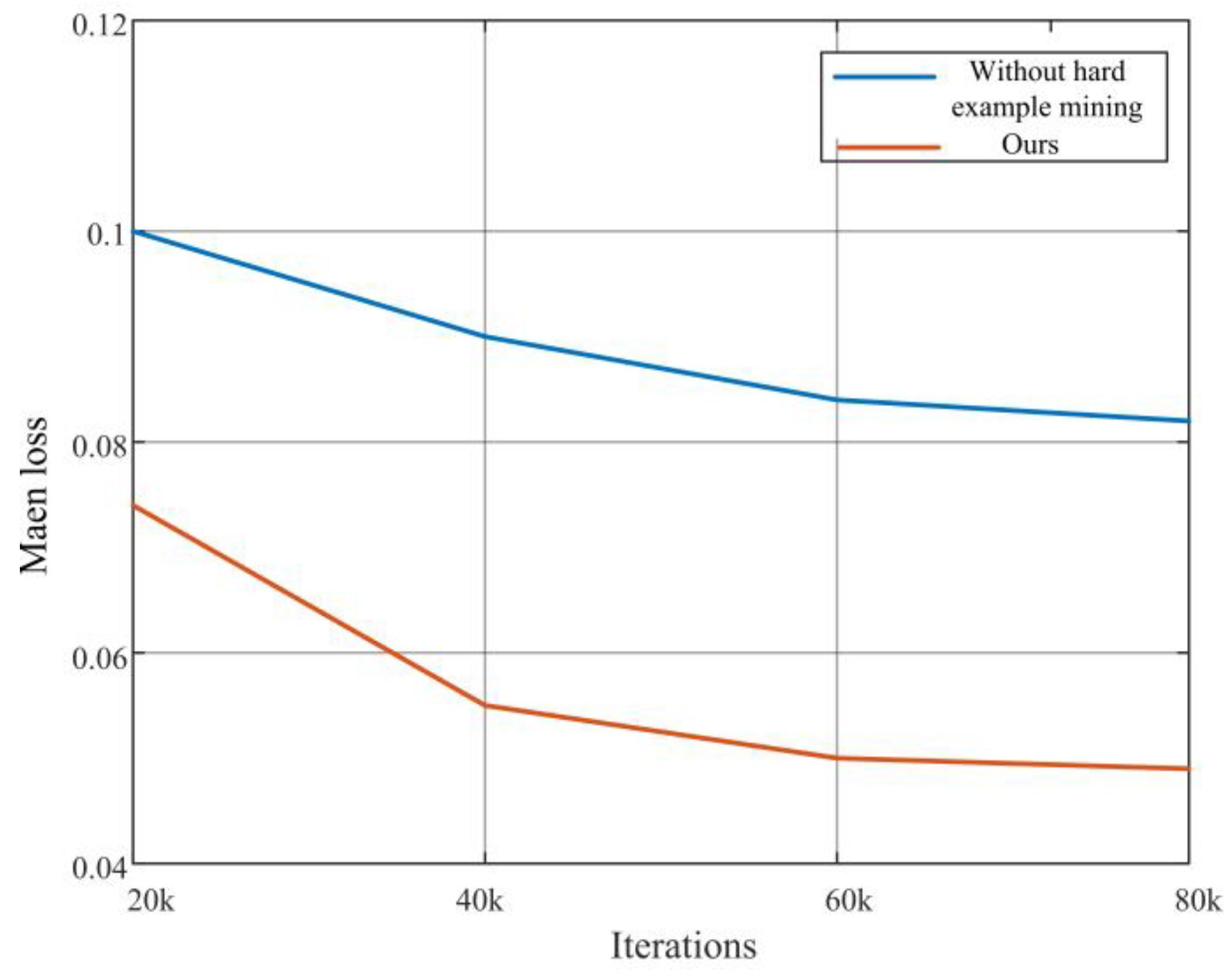
2.2.4. Hard Example Mining

The sample training set always contains a large proportion of easy examples and a few hard examples, of which the former have little training significance and the latter, characterized by diversity and high loss values, have a considerable impact on the classification and detection results. Utilizing these hard examples can enhance the discrimination ability of the network based on the object. The issue of category imbalance is not a new challenge, and the idea of dataset bootstrapping [27] has been successfully applied in the training process of many detection tasks. This method is also known as hard example mining. Recently, the A-Fast-RCNN object detection model [28], which uses generative adversarial nets to produce occlusion and deformation examples, is also regarded as an example mining approach. Example mining is most important for airports with limited data. Thus, in this study, the concept of hard example mining is employed to make example training more efficient. The overall structure of the method is shown in Figure 6.

We propose a simple yet effective hard example mining algorithm for training detection networks. The alternating steps are: (a) for some period of time a fixed model is used to find new examples to add to the active training set; (b) then, the model is trained on the fixed active training set. More specifically, the original detection network is duplicated into two sets designated Network A and Network B, which share network parameters. Network A involves only forward operations, and Network B is a standard detection network with both forward and backward operations.

The flowchart of the hard example mining is shown in Figure 7. First, for an input image at stochastic gradient descent (SGD) iteration, t, a convolutional (conv) feature map is computed by using the conv network. Second, the corresponding feature maps are generated for their respective candidate regions, instead of a sampled mini-batch, through RoI pooling layers, and then outputted to Network A for forward transfer and the calculation of the loss value. This step only involves RoI pooling layer, fully connected layers, and loss computation. The loss represents the current network’s execution of each candidate region. Third, the hard example sampling module sorts the loss values of all the candidate regions and selects $B/N$ examples for which the current network performs worst. Finally, $B/N$ hard examples are outputted to Network B for normal model training. The input to Network A is all the candidate regions $P$ of $N$ images rather than the mini-batch $B$, and the batch input to Network B is $B$. Most forward calculations are shared between candidate regions, so the extra calculations required to forward all candidate regions are relatively small. In addition, since only a small amount of candidate regions is selected to update the model, the backward pass is not more expensive than before.

2.3. Network Training

To overcome training difficulty issues and avoid overfitting due to small sample sizes, the weights of the shared convolutional layers are initialized with the pretraining network VGG16, and the weights of the remaining layers are initialized based on a Gaussian distribution with a mean of 0 and a standard deviation of 0.01. The basic learning, momentum and weight decay coefficients of the network are 0.001, 0.9, and 0.0005, respectively. To enable the sharing of convolutional layers between the cascade RPNs and multi-threshold detection networks, an alternate optimization strategy is adopted to train the entire network in four steps.

Step 1 involves training the cascade RPNs and outputting the airport candidate box sets. After the initialized candidate boxes of the pretraining network VGG16 generate network weights, end-to-end fine-tune training is performed. After the training is completed, the airport candidate box sets are outputted.

Step 2 involves training the candidate box detection network. After the network weights are tested by the initialized candidate boxes of network VGG16, the airport candidate boxes generated in Step 1 are used to train the multi-threshold detection network. At this time, the two networks do not share convolutional layers.

Step 3 involves fine tuning the cascade RPNs and outputting the airport candidate box sets. The cascade RPNs are initialized using the final weights of the detection network obtained from Step 2 to set the weights of the shared convolutional layers, and only the layers unique to the cascade RPNs are fine tuned. After training is completed, the airport candidate box sets are outputted. During this process, the two networks share convolutional layers.

Step 4 involves fine tuning the training network model again. The weight parameters of the shared convolutional layers and cascade RPNs are kept constant, the fully connected layers of the detection network are tuned using the airport candidate boxes outputted in Step 3, and ultimately, the convolution layer-sharing airport detection network is obtained.

3. Results

3.1. Dataset and Computational Platform

The experimental data are from Google Earth, and the original images, all of which are 600 × 600 pixels in size, are of 300 airports in locations around the world. The training validation set is composed of 1000 airport images, which are obtained through data expansion of the 200 original airport images; another 100 original airport images are used as the test set. The airport data set is formed in reference to the standard data set V0C 2007. To prevent overfitting, the images are flipped at a probability of 0.5 during training. The experimental environment included an i7-7700 processor running at 3.6 GHz, 16 G of memory, and an NVIDIA GTX1080 (graphics card). All the results in the experiment are averages from multiple random experiments.

The number of remote sensing images is very limited, and these data are not labeled with type information. End-to-end methods can achieve good performance, but they need large numbers of labeled samples. However, limited by the quantity of labeled data in remote sensing images, they suffer from bad generation performance. It is obvious that the amount of labeled data has become an important factor blocking end-to-end methods development. Thus, we must artificially expand the training data and label them. Common data expansion methods include horizontal/vertical flipping, rotation/reflection, cropping, zooming, shifting, scaling, noise adjustment, and contrast adjustment. These methods are implemented to expand the data through the built-in Image Data Generator in Keras. Keras is a high-level neural networks API, written in Python and capable of running on top of TensorFlow, CNTK, or Theano. It was developed with a focus on enabling fast experimentation. Being able to go from idea to result with the least possible delay is key to doing good research. For airport objects, rotation, shifting and vertical flipping are used to expand airport images, in which all the operations are randomly adopted, as shown in Figure 8. Specifically, Figure 8a shows the original image, and Figure 8b shows the images after data expansion.

3.2. Results on Test Set

The detection rate (DR) and false alarm rate (FAR) are used to evaluate the performance of the model and are defined, respectively, as follows:

$$DR=\frac{number\hspace{1em}of\hspace{1em}detected\hspace{1em}airports}{number\hspace{1em}of\hspace{1em}ariports}\times 100\%=\frac{TP}{TP+FN}\times 100\%$$

(10)

$$FAR=\frac{number\hspace{1em}of\hspace{1em}False\hspace{1em}Alarms}{number\hspace{1em}of\hspace{1em}detected\hspace{1em}objects}\times 100\%=\frac{FP}{TP+FP}\times 100\%$$

(11)

Here TP denotes the number of true positive samples; TNdenotes the number of true negative samples; FP denotes the number of false positive samples; and FN denotes the number of false negative samples. The intersection-over-union (IoU) is calculated by the detected bounding box and the ground-truth of objects. If IoU is bigger than 0.5, we considered that the airport is detected. In addition, the average processing time is adopted to evaluate the computational speed of the algorithms. The run time for the algorithm in five trials was recorded and averaged.

Figure 9 shows some of the test results using the method developed in this study. In these experiments, the airport background includes roads, buildings, rivers, mountains, and other features, and in the bottom row, airport images with some unique shapes are shown. The test results show that the airport regions in the images are all accurately identified, which indicates that the proposed method can accurately detect airports with a variety of complex backgrounds.

To prove the superiority of the proposed method to traditional methods, existing airport detection methods are selected for comparative experiments. Based on the available software code for other airport detection methods, simulation experiments of these methods were conducted in the experimental environment of this study, and the DR, FAR, and average run time of each method were recorded and then compared. The comparison results are shown in

Table 2. Comparison of the results of different methods.

Method	Detection Rate (DR) (%)	False Alarm Rate (FAR) (%)	Average Processing Time (s)
Method 1	65	27.8	2.6
Method 2	71	27.6	>100
Method 3	83	29.7	21.3
Method 4	90	9.6	0.2
Faster R-CNN	88	15.5	0.2
Our method	95	6.9	0.2

. Of these methods, method 1 [8] is an edge-based airport detection method, method 2 [13] is an airport detection method based on region segmentation, and method 3 [16] is an airport detection method based on CNN. In addition, Faster R-CNN refers to the results obtained by a Faster R-CNN method after transfer learning based on the airport database and the modification of the corresponding parameters. Method 4 [29] uses Faster R-CNN algorithm with some specific improvements.

Table 2 shows that the performance of Faster R-CNN and the method proposed in this study are superior to that of the other methods. Of the methods considered, the method proposed in this study has the highest DR, the lowest FAR, and the shortest average run time.

The work in [8] utilizes the segmentation of images to extract statistical information and Hough transforms to get the line features, so it is very sensitive to complex lines. The work in [13] relies on sift features to determine candidate regions, but the sift features that some airports can extract are very limited, and the robustness of sift features is also not strong. All in all, reference [8] and reference [13] use sliding windows and manually designed features to achieve airport detection. The weakness of the manually designed features, including edge and textures, lies in the difficulties of finding proper representations through uncertain experience and limited expert knowledge. Because the calculation efficiency of the sliding window through image traversal is very low and the robustness of the manually designed features is not strong, their detection results are not satisfactory. The work in [16] introduces an airport detection method using deep CNN with a line-based region proposal method. Because deep CNNs could learn rich highly abstract features to represent objects effectively, Reference [16] could significantly improve the DR. However, because it extracts region proposal through line segment detection based on prior knowledge, its detection performance is limited, especially in regard to the detection time. Faster R-CNN, reference [29] and our method integrate feature extraction, candidate box selection, and object classification and regression in an end-to-end deep network framework, which fully uses the powerful feature representation ability of the CNN. Additionally, the RPN and detection network share convolutional layers, thereby greatly improving the accuracy and speed of airport detection. Therefore, their detection performance is far superior to the previous method, especially relating to the detection time. The work in [29] increased detection performance by adding additional scale and aspect ratios compared to Faster R-CNN. However, we use the cascade RPN, multi-threshold detection networks and hard examples to improve the Faster R-CNN algorithm. The experimental results show that our improvements are better than those of reference [29]. In summary, our method outperforms previous airport detection methods.

4. Discussion

4.1. Sensitivities to Parameters

In

Table 3. Detection results using different pretraining networks.

Method	DR/%	Average Run Time/s
ZFNet	83	0.051
VGG_CNN_M_1024	87	0.062
VGG16	95	0.124

we compare the DR with different pretraining networks: Zeiler Fergus Network (ZF Net), VGG_CNN_M_1024 and VGG16. In order to compare the time more accurately, the time value is accurate to 3 decimal places. As the level of the network structure deepens, the performance of the algorithm increases, but the time also increases. Therefore, considering the detection rate and time overall, VGG16 is selected as the pretraining network.

In

Table 4. Detection results using different settings of anchors.

Settings	Anchor Scales	Aspect Ratios	DR (%)
1 scale, 1 ratio	1282 2562	1:1 1:1	91 91
1 scale, 3 ratio	1282 2562	(1:1, 2:3, 3:2) (1:1, 2:3, 3:2)	94 93
3 scale, 3 ratio	(1282, 1982, 2562)	(1:1, 2:3, 3:2)	95

we investigate the settings of anchors. By default, we use three scales and three aspect ratios (95% DR in Table 4). If using just one anchor at each position, the DR drops by a considerable margin (of 2–3%). The DR is higher if using three scales (with one aspect ratio) or three aspect ratios (with one scale), demonstrating that using anchors of multiple sizes as the regression references is an effective solution.

In

Table 5. Detection results using different values of $\lambda$.

λ	0.1	1	10	100
DR (%)	93	94	95	94

we compare the results arising from different values of the parameter $\lambda$ in Equation (2). In order to make the two terms in Equation (2) roughly equally weighted after normalization, by default we use $\lambda =10$. Table 5 shows that our results are only slightly affected when $\lambda$ is within the range of about two orders of magnitude (1 to 100). This indicates that the results are insensitive to a wide range of $\lambda$.

4.2. Analysis of Improvement

To verify the effectiveness of the cascade RPN, the improved loss function, and the hard example mining method, comparative experiments were conducted using the controlled variable method.

The results of the comparison experiments involving the region proposal methods are shown in

Table 6. Results of different region proposal methods.

Method	RPN	Cascade RPN
DR (%)	88	91
Average processing time (s)	0.121	0.124

. The cascade RPN significantly improves DR (by 3%) without increasing computational time. Because an RPN uses very little time for all network processes, the time required by a cascade RPN is negligible.

The comparison experiment results involving the loss function are shown in Figure 10. The X-axis is the IoU threshold during image testing, and the Y-axis is the corresponding DR. Here, $g=50$ represents the IoU threshold of the loss function in Equation (5), which is constant at 0.5. The results show that the DR of the method developed in this study is always higher than that of the model method that corresponds to $g=50$, and the difference between the two methods gradually increases as the IoU threshold increases. This result indicates that the improved loss function leads to more accurate positioning that enables the model to achieve a higher DR, and as the IoU threshold increases, the positioning advantage becomes increasingly profound.

During the model training process, the average loss value (i.e., the mean of the loss functions of all candidate regions) is recorded every 20,000 iterations, and the comparison experiment is performed on the test set. The results are shown in Figure 11 and Table 5.

Figure 11 shows that during the entire training process, the model with hard example mining has a low loss value, which indicates that the hard example mining method can effectively reduce the loss value of the training process and make model training more efficient.

Table 7. Comparison of the results.

Method	DR (%)	Average Run Time (s)
Without hard example mining	88	0.124
Method proposed in this study	92	0.124

shows that the hard example mining method improves DR by approximately 4% without increasing computational time. Notably, in the training process, hard examples are fully utilized in this method, which makes model training more efficient; hard example mining increases the training time of the model but does not affect the detection time.

4.3. Application to Aircraft

As an important object in the airport, the aircraft is also of interest; thus, we have also applied the model to airplane detection. All airplane images are collected from satellite images of 300 of the world’s airports in Google Earth, with a spatial resolution of 1.19 m. Aircraft images from 150 airports are selected as training and verification sets with a total of 1500 images; their sizes ranged from 375 × 375 to 400 × 400. The aircraft images in the remaining 150 airports are used as test sets, with image sizes between 900 × 800 and 1000 × 900. The detection results on the airplane test images are shown in Figure 12. Figure 12 shows that the method of this paper can be applied to airplane detection. On our computational platform, it takes about 0.139 s to process an image with a detection rate of 90.28% and a false alarm rate of 11.6%.

5. Conclusions

In this study, we designed an end-to-end airport detection method for remote sensing images using a region-based convolutional neural network as the basic framework. In this method, transfer learning of the pretraining network is used to solve the problem of inadequate airport image data, and the cascade RPNs improve the quality of the candidate boxes through further screening and optimizing the candidate boxes. After fully accounting for the influence of the IoU training threshold on the positioning accuracy, the multi-threshold detection networks are proposed, which ultimately enhance DR. Mining hard examples makes training more efficient, and the sharing of convolutional layers between the cascade RPNs and the detection networks during model training greatly improves the efficiency of airport detection. The experimental results show that the method proposed in this study can accurately detect various types of airports in complex backgrounds, and that it is superior to existing detection methods. A gap remains between the processing speed and instantaneity, which will be the focus of our future studies. Nonetheless, the proposed method is of theoretical and practical significance for real-time and accurate airport detection.

In this paper, using the Faster R-CNN algorithm as the basic framework, we achieved state-of-the-art detection accuracy and computational speed. In addition, there would be value in testing other CNN-based object detection algorithms, such as You Only Look Once (YOLO) and Single Shot Detector (SSD). This will also be a topic of our future research work.

References

1. Zhu, X.X.; Tuia, D.; Mou, L.; Xia, G.-S.; Zhang, L.; Xu, F.; Fraundorfer, F. Deep Learning in Remote Sensing: A Comprehensive Review and List of Resources. IEEE Trans. Geosci. Remote Sens. 2017, 5, 8–36. [Google Scholar] [CrossRef] [Green Version]
2. Jin, X.; Davis, C.H. Vehicle detection from high-resolution satellite imagery using morphological shared-weight neural networks. Image Vis. Comput. 2007, 25, 1422–1433. [Google Scholar] [CrossRef]
3. Chen, X.; Xiang, S.; Liu, C.-L.; Pan, C.-H. Vehicle detection in satellite images by hybrid deep convolutional neural networks. IEEE Geosci. Remote Sens. Lett. 2014, 11, 1797–1807. [Google Scholar] [CrossRef]
4. Zhang, L.; Shi, Z.; Wu, J. A hierarchical oil tank detector with deep surrounding features for high-resolution optical satellite imagery. IEEE J. Sel. Top. Appl. Earth Obs. Remote Sens. 2015, 8, 886–893. [Google Scholar] [CrossRef]
5. Zhang, F.; Du, B.; Zhang, L.; Xu, M. Weakly supervised learning based on coupled convolutional neural networks for aircraft detection. IEEE Trans. Geosci. Remote Sens. 2016, 54, 5553–5563. [Google Scholar] [CrossRef]
6. Tang, J.; Deng, C.; Huang, G.-B.; Zhao, B. Compressed-domain ship detection on spaceborne optical image using deep neural network and extreme learning machine. IEEE Trans. Geosci. Remote Sens. 2015, 53, 1174–1185. [Google Scholar] [CrossRef]
7. Liu, D.; He, L.; Carin, L. Airport Detection in Large Aerial Optical Imagery. In Proceedings of the IEEE International Conference on Acoustics, Speech and Signal Processing, Montreal, QC, Canada, 17–21 May 2004; pp. 761–764. [Google Scholar]
8. Qu, Y.; Li, C.; Zheng, N. Airport Detection Base on Support Vector Machine from a Single Image. In Proceedings of the IEEE International Conference on Signal Processing, Bangkok, Thailand, 6–9 December 2005; pp. 546–549. [Google Scholar]
9. Bhagavathy, S.; Manjunath, B.S. Modeling and Detection of Geospatial Objects Using Texture Motifs. IEEE Trans. Geosci. Remote Sens. 2006, 44, 3706–3715. [Google Scholar] [CrossRef]
10. Aytekin, O.; Zongur, U.; Halici, U. Texture-based Airport Runway Detection. IEEE Geosci. Remote Sens. Lett. 2013, 10, 471–475. [Google Scholar] [CrossRef]
11. Tang, G.; Xiao, Z.; Liu, H. A Novel Airport Detection Method via Line Segment Classification and Texture Classification. IEEE Geosci. Remote Sens. Lett. 2015, 12, 2408–2412. [Google Scholar] [CrossRef]
12. Budak, U.; Halici, U.; Sengur, A.; Karabatak, M.; Xiao, Y. Efficient Airport Detection Using Line Segment Detector and Fisher Vector Representation. IEEE Geosci. Remote Sens. Lett. 2016, 13, 1079–1083. [Google Scholar] [CrossRef]
13. Tao, C.; Tan, Y.; Tian, J. Airport Detection From Large IKONOS Images Using Clustered SIFT Keypoints and Region Information. IEEE Geosci. Remote Sens. Lett. 2011, 8, 128–132. [Google Scholar] [CrossRef]
14. Zhu, D.; Wang, B.; Zhang, L. Airport target detection in remote sensing images: A new method based on two-way saliency. IEEE Geosci. Remote Sens. Lett. 2015, 12, 1096–1100. [Google Scholar]
15. Zhang, P.; Niu, X.; Dou, Y. Airport detection from remote sensing images using transferable convolutional neural networks. In Proceedings of the International Joint Conference on Neural Network, Budapest, Hungary, 14–19 July 2016; pp. 2590–2595. [Google Scholar]
16. Zhang, P.; Niu, X.; Dou, Y.; Xia, F. Airport detection on optical satellite images using deep convolutional neural networks. IEEE Geosci. Remote Sens. Lett. 2017, 14, 1183–1187. [Google Scholar] [CrossRef]
17. Xiao, Z.F.; Gong, Y.P.; Long, Y. Airport Detection Based on a Multiscale Fusion Feature for Optical Remote Sensing Images. IEEE Geosci. Remote Sens. Lett. 2017, 14, 1469–1473. [Google Scholar] [CrossRef]
18. Girshick, R.; Donahue, J.; Darrell, T.; Malik, J. Rich Feature Hierarchies for Accurate Object Detection and Semantic Segmentation. In Proceedings of the IEEE Conference on Computer Vision and Pattern Recognition, Columbus, OH, USA, 23–28 June 2014; pp. 580–587. [Google Scholar]
19. Girshick, R. Fast R-CNN. In Proceedings of the IEEE Conference on Computer Vision and Pattern Recognition, Santiago, Chile, 13–16 December 2015; pp. 1440–1448. [Google Scholar]
20. Ren, S.; He, K.; Girshick, R.; Sun, J. Faster R-CNN: Towards real-time object detection with region proposal networks. In Proceedings of the Advances in Neural Information Processing Systems, Montreal, QC, Canada, 7–12 December 2015; pp. 91–99. [Google Scholar]
21. Uijlings, J.; Van de Sande, K.; Gevers, T.; Smeulders, A. Selective Search for Object Recognition. Int. J. Comput. Vis. 2013, 104, 154–171. [Google Scholar] [CrossRef] [Green Version]
22. Pan, S.; Yang, Q. A Survey on Transfer Learning. IEEE Trans. Knowl. Data Eng. 2010, 22, 1345–1359. [Google Scholar] [CrossRef] [Green Version]
23. Simonyan, K.; Zisserman, A. Very Deep Convolutional Networks for Large-Scale Image Recognition. arXiv. 2015. Available online: http://arxiv.org/abs/1409.1556 (accessed on 10 April 2015).
24. Deng, J.; Dong, W.; Socher, R. Imagnet: A large-scale hierarchical image database. In Proceedings of the 2009 IEEE Conference on Computer Vision and Pattern Recognition, Miami, FL, USA, 20–25 June 2009. [Google Scholar]
25. Yan, J.; Yu, Y.; Zhu, X. Object detection by labeling superpixels. In Proceedings of the IEEE Conference on Computer Vision and Pattern Recognition, Santiago, Chile, 13–16 December 2015; pp. 5107–5116. [Google Scholar]
26. Kuo, W.; Hariharan, B.; Malik, J. DeepBox: Learning Objectness with Convolutional Network. In Proceedings of the IEEE Conference on Computer Vision and Pattern Recognition, Santiago, Chile, 13–16 December 2015; pp. 2479–2487. [Google Scholar]
27. Felzenszwalb, P.; Girshick, R.; Mcallester, D. Object Detection with Discriminatively Trained Part-Based Models. IEEE Trans. Pattern Anal. Mach. Intell. 2010, 32, 1627–1645. [Google Scholar] [CrossRef] [PubMed] [Green Version]
28. Wang, X.; Shrivastava, A.; Gupta, A. A-Fast -CNN: Hard Positive Generation via Adversary for Object Detection. In Proceedings of the IEEE Conference on Computer Vision and Pattern Recognition, Honolulu, HI, USA, 21–26 July 2017. [Google Scholar]
29. Chen, F.; Ren, R.; Van de Voorde, T.; Xu, W.; Zhou, G.; Zhou, Y. Fast Automatic Airport Detection in Remote Sensing Images Using Convolutional Neural Networks. Remote Sens. 2018, 10, 443. [Google Scholar] [CrossRef]
Figure 1. The airport detection network architecture is shown in the blue frame, and the cascade region proposal network architecture is shown in the green frame.
Remotesensing 10 01516 g001
Figure 2. Schematic diagram of the Faster R-CNN.
Remotesensing 10 01516 g002
Figure 3. Schematic diagram of the RPNs.
Remotesensing 10 01516 g003
Figure 4. Schematic diagram of transfer learning.
Remotesensing 10 01516 g004
Figure 5. The structure of the cascade RPNs.
Remotesensing 10 01516 g005
Figure 6. The overall structure of the method used in this study.
Remotesensing 10 01516 g006
Figure 7. The flowchart of hard example mining.
Remotesensing 10 01516 g007
Figure 8. Schematic diagram of data expansion.
Remotesensing 10 01516 g008
Figure 9. Various airport detection results.
Remotesensing 10 01516 g009
Figure 10. Results with different loss functions.
Remotesensing 10 01516 g010
Figure 11. Comparison of the loss values.
Remotesensing 10 01516 g011
Figure 12. Detection results in airplane images.
Remotesensing 10 01516 g012