Impact of the Acquisition Geometry of Very High-Resolution Pléiades Imagery on the Accuracy of Canopy Height Models over Forested Alpine Regions

Abstract

This work focuses on the accuracy estimation of canopy height models (CHMs) derived from image matching of Pléiades stereo imagery over forested mountain areas. To determine the height above ground and hence canopy height in forest areas, we use normalised digital surface models (nDSMs), computed as the differences between external high-resolution digital terrain models (DTMs) and digital surface models (DSMs) from Pléiades image matching. With the overall goal of testing the operational feasibility of Pléiades images for forest monitoring over mountain areas, two questions guide this work whose answers can help in identifying the optimal acquisition planning to derive CHMs. Specifically, we want to assess (1) the benefit of using tri-stereo images instead of stereo pairs, and (2) the impact of different viewing angles and topography. To answer the first question, we acquired new Pléiades data over a study site in Canton Ticino (Switzerland), and we compare the accuracies of CHMs from Pléiades tri-stereo and from each stereo pair combination. We perform the investigation on different viewing angles over a study area near Ljubljana (Slovenia), where three stereo pairs were acquired at one-day offsets. We focus the analyses on open stable and on tree covered areas. To evaluate the accuracy of Pléiades CHMs, we use CHMs from aerial image matching and airborne laser scanning as reference for the Ticino and Ljubljana study areas, respectively. For the two study areas, the statistics of the nDSMs in stable areas show median values close to the expected value of zero. The smallest standard deviation based on the median of absolute differences (σ_MAD) was 0.80 m for the forward-backward image pair in Ticino and 0.29 m in Ljubljana for the stereo images with the smallest absolute across-track angle (−5.3°). The differences between the highest accuracy Pléiades CHMs and their reference CHMs show a median of 0.02 m in Ticino with a σ_MAD of 1.90 m and in Ljubljana a median of 0.32 m with a σ_MAD of 3.79 m. The discrepancies between these results are most likely attributed to differences in forest structure, particularly tree height, density, and forest gaps. Furthermore, it should be taken into account that temporal vegetational changes between the Pléiades and reference data acquisitions introduce additional, spurious CHM differences. Overall, for narrow forward–backward angle of convergence (12°) and based on the used software and workflow to generate the nDSMs from Pléiades images, the results show that the differences between tri-stereo and stereo matching are rather small in terms of accuracy and completeness of the CHM/nDSMs. Therefore, a small angle of convergence does not constitute a major limiting factor. More relevant is the impact of a large across-track angle (19°), which considerably reduces the quality of Pléiades CHMs/nDSMs.

1. Introduction

Mountain forests provide a wide range of ecosystem services in terms of protective, productive, social and economic functions. Therefore, the timely information on the state and the change of land-use and forest cover, productivity, and structure is crucial for different stakeholders from local to regional scales. To quantify the provided forest services, detailed forest information is required with high spatial and temporal resolutions. Among the forest metrics, canopy height, which describes the top of the vegetated canopy, is the basis for deriving other parameters such as forest gaps, crown coverage, canopy density, volume, and biomass. For deriving canopy height at wide spatial coverage i.e., at the landscape scale, remote sensing observations with fine spatial resolutions are required. Current remote sensing systems that fulfil this requirement include airborne laser scanning (ALS) and multi-view aerial or very high resolution (VHR) satellite imagery [1]. Since the last decade, airborne laser scanning (ALS) has been the primary data source for three-dimensional (3D) information on forest vertical structure [2,3,4]. The main advantage of ALS for forest applications is the capability to penetrate through the vegetation and thus to obtain the top height, the forest vertical structure, and the bare-earth, with the latter being needed to define the terrain height. By contrast, passive optical sensors can provide only the topmost surface of forest canopies, where at least two images (a so-called image stereo pair) share a common area in the scene [5]. Both aerial and satellite images have been used to record forest change for more than 30 years. In the last decade, thanks to great technological improvements, the gap between aerial and VHR satellite imagery has become smaller in terms of image resolution (up to 30 cm ground sample distance (GSD)). However, in comparison with airborne remote sensing, VHR satellite imagery has the benefits of worldwide availability without any access restrictions, large area coverage and high temporal resolutions of only a few days.

Forest mapping over large spatial extents with VHR satellites started with IKONOS in 1999 [6,7]. Since then, several VHR satellites have been launched such as QuickBird, GeoEye-1, WorldView-1, -2, and -3, Ziyuan-3A, and the Pléiades satellites. WorldView multispectral stereo imagery was largely used to analyse forest structure [8,9], the size of tree crowns [10] and for the 3D modelling of forest canopies [1,11,12].

Among the available VHR satellite systems, we consider Pléiades imagery over mountain regions for deriving DSMs. This first European VHR satellite system is comprised of two identical satellites, Pléiades-1A (PHR1A) and Pléiades-1B (PHR1B), which were launched in December 2011 and in December 2012, respectively. Both satellites fly at an altitude of 694 km in sun-synchronous orbits with 98.2° inclination and an offset of 180° from each other, which provides a daily revisit capability [13]. An outstanding feature of the Pléiades system is the great agility of its sensors that allows for optimised acquisitions of areas of interest, with stereo angles varying from ~6° to ~28° [14]. The time difference between along-track images is in the range of a few seconds only, which guarantees almost constant sun illumination conditions, limited changes in the scene and similar cloud coverages in all of them [15]. Moreover, the sensor is designed to acquire panchromatic and multispectral images, which are delivered at nominal resolutions of 0.5 m and 2 m, respectively, in stereo (forward-, backward-view) and tri-stereo (forward-, nadir-, and backward-view) modes along-track.

To explore the full potential of Pléiades images over forest mountain areas, an investigation of the relationship between DSM accuracy and imaging geometry, such as tri-stereo imagery, convergence angle and across-track angle, is essential for an optimal image acquisition planning. Therefore, we focus on answering the question of which combination and acquisition setting of tri-stereo or stereo pairs of Pléiades images can produce the highest DSM accuracy over Alpine forest regions.

Related Work and Research Questions

Despite the advantages of the Pléiades system, only a limited number of studies have investigated the versatility of the Pléiades system through the controllable viewing angle and stereo and tri-stereo views for forestry applications. The generation of height models with Pléiades triplets with large and short base length image combinations has been investigated in different urban areas by References [16,17,18,19]. In Alpine areas, the capability of Pléiades tri-stereo to deliver reliable DSMs in complex terrain was demonstrated by References [20,21,22]. Additionally, the benefit of using tri-stereo images was tested to estimate the lava flow volume [12], and the height changes induced by earthquakes [23]. Among the few researchers that have used the Pléiades satellites for forestry purposes, the Pléiades image texture for forest structure mapping and forest classification has been investigated previously in [24,25]. Recently, the potential for use Pléiades images has been investigated for estimating forest attributes for 10 m plots in a boreal forest [26], for deriving forest biomass by combining spectral and geometric information [27,28], for predicting forest inventory attributes in New Zealand’s planted forests [29] and for modelling tree diversity [30].

In contrast to these previous works on the use of Pléiades satellite images over forest areas, our study is, to the best of our knowledge, the first to explore the accuracy of DSMs/CHMs derived from Pléiades imagery over large mountain regions. Specifically, our work aims at answering the following two questions, both regarding the accuracy of derived DSMs: (1) what is the benefit of using tri-stereo images versus stereo pairs, and (2) what is the impact of different viewing angles and topography? According to this twofold goal, the investigation is carried out in two accordingly selected study areas located in Alpine forest regions. In order to derive the height above ground (nDSM), we subtract external high resolution DTMs from Pléiades image matching DSMs. We focus the analyses of the nDSMs/CHMs on open stable areas, and on tree covered areas. For evaluating the accuracy of Pléiades CHMs, we use CHMs from aerial image matching and ALS as reference for the Ticino and Ljubljana study areas, respectively.

2. Test Sites and Pléiades Image Data Sets

We tasked a new tri-stereo Pléiades data acquisition over Canton Ticino, Switzerland (site “Ticino”) to investigate the potential of triplet scenes and the impact of tree height and slope on CHM accuracy in forest mountain areas. The area was chosen for its topographic characteristics, with elevations between 220 m and 2265 m a.s.l. and an average slope of 37°. The tri-stereo data were acquired with platform PHR1A within 20 s on 3 September 2017 around 10:00 in North-South direction, covering ~125 km² in total (Figure 1). To study the impact of different along- and across-track angles, we used three Pléiades stereo pairs near Ljubljana, Slovenia (site “Ljubljana”) available in the supplier’s archive, which were acquired one day apart from each other with platform PHR1A on 27 and 29 July 2013, and with platform PHR1B on 28 July 2013. This study area is rather flat with elevations between 346 m and 1900 m a.s.l., and an average slope of 8.6°. It comprises about 400 km² that largely consist of agricultural land and managed forest.

The optical satellite images for both study areas were delivered as four bands (blue, green, red, near infrared), pan-sharpened with spatial resolutions (i.e., mean GSDs) between 0.71 m and 0.78 m, depending on the viewing angle. The viewing angles and consequently the convergence angles and baseline to height ratios are different for each stereo pair. For the Ticino dataset, according to our request, we received one quasi-nadir image (viewing angle close to the vertical), and one backward- and one forward-view with symmetric along-track angles, and a small convergence angle of about 12°. The archive images over Slovenia were collected in stereo mode with symmetric and asymmetric along-track angles and rather large convergence angles. In the across-track direction, the mean angles are −5.3°, 6.8°, and 19.6°. The acquisition properties of the satellite images for each study area are given in

Table 1. Acquisition properties for the satellite images over the two study areas.

Study Area	Acquisition Date	View	Acqu. Time	GSD (m)	Incidence Angles (°)
				Along Track	Along Track	Across Track	Angle of Convergence
Ticino	3 September 2017	Forward	10:29:03	0.71	6.05	−0.42	5 (FN)
		Nadir	10:29:13	0.70	0.89	0.78	6 (NB)
		Backward	10:29:22	0.70	−5.37	2.49	12 (FB)
Ljubljana	27 July 2013	Forward	10:10:09	0.73	−12.12	−1.98	24
		Backward	10:10:51	0.74	12.36	−8.59
	28 July 2013	Forward	10:03:43	0.71	−7.39	9.36	22
		Backward	10:04:21	0.74	14.78	3.95
	29 July 2013	Forward	09:55:04	0.77	−10.20	22.31	27
		Backward	09:55:50	0.78	16.91	16.90

. Figure 1 shows the Pléiades satellite positions over Ticino and Ljubljana.

3. Data Processing and Analyses

3.1. Reference Data

For Ticino, an aerial image matching DSM [31] was used as reference data. The aerial images were acquired in spring 2015 (two years before the Pléiades images) and the corresponding DSM was provided by the Swiss National Forest Inventory as a raster with 1 m resolution. The digital terrain model swissAlti3D from the Federal Office of Topography (swisstopo) with a resolution of 2 m was upsampled to 1 m and was used to derive the Pléiades and Aerial nDSM and to improve the absolute geolocation of the Pléiades DSMs (see Section 3.2.2). The reference data in Slovenia was based on ALS data collected in 2015 (i.e., two years after the Pléiades images), having a mean density of 14 points/m². From the classified ALS point cloud, the DTM and the nDSM were derived with a resolution of 1 m using OPALS [32]. For both study areas, an existing orthophoto of 0.2 m spatial resolution was used to pick the ground control points (GCPs) and check points (CPs) over stable areas, whose height coordinates were extracted from the corresponding DTM. The GCPs were used in the image orientation phase to optimize the Pléiades projection parameters provided along with the image data, whereas the purpose of the CPs was to validate the accuracy of the image orientations and the DSMs. The GCPs and CPs were homogeneously distributed in planimetry and height across the area. The accuracies of the measured GCP and CP object coordinates were in the order of 20 cm in planimetry and 25 cm in the vertical direction.

3.2. Pléiades Image Processing and DSM Generation

3.2.1. Pléiades Image Processing

The reconstruction of 3D points from VHR satellite imagery requires at least two overlapping images, and it is performed by applying photogrammetric techniques and dense image matching algorithms. The transformation between image and object space is given in terms of the Rational Polynomial Coefficients (RPCs) model [33]. The RPCs are provided for each image by the satellite vendor. For the Pléiades pan-sharpened imagery the RPCs are reported to have a geo-location accuracy of 8.5 m CE90 (circular error at 90% confidence) for nadir view in the nadir direction, which corresponds to a standard deviation of 4 m [34]. Therefore, the declared absolute accuracy is not sufficient if sub-meter accuracy is required, but this can be achieved with the use of GCPs. Thus, in total, we employed 18 GCPs for each study area and 7 and 12 CPs for Ticino and Ljubljana, respectively. Additionally, in order to quantify the geolocation accuracy of the original RPCs, the tri-stereo images over Ticino were also evaluated without GCPs.

The Pléiades images were processed using Trimble/Inpho software. To generate a 3D point cloud from stereo imagery the main procedure is (i) to import the images and the RPC information, (ii) to (optionally) refine the orientation of the images based on tie points and GCPs, and (iii) to apply dense image matching to determine the dense point cloud. The general workflow from the images to the final DSM is illustrated in Figure 2.

For each study area, the image orientation refinement was performed jointly for all available images in order to minimize the influence of the image orientation quality on the quality of the DSMs derived for particular combinations of images. Therefore, tie points were extracted automatically for all images, and they were employed together with the GCPs to refine the initial RPC coefficients. During bundle block adjustment, the residuals of tie points, GCPs, and CPs were computed by the software. Consequently, tie points with image residuals larger than 2 pixels were considered as blunders and removed, and the RPCs refined again. For dense image matching, Match-T was used. This is a module of the Trimble/Inpho software, which adopts a feature-based on the higher and a cost-based strategy on the lower pyramid levels. The cost-based matching is a version similar to the semi-global matching algorithm [35], which computes an object point for every pixel. For the Ticino study area, after a simultaneous orientation refinement of the tri-stereo images, dense matching was performed independently for the tri-stereo data (forward, nadir, backward, FNB) and for each stereo pair i.e., forward-nadir (FN), nadir-backward (NB), and forward-backward (FB). A similar approach was adopted for the Ljubljana study area. Thus, the six images were jointly oriented based on tie points and GCPs, and dense matching was performed for the forward-backward pair of each day of acquisition. For both study areas, four band orthophotos were generated to derive normalised difference vegetation index (NDVI) maps.

3.2.2. Pléiades DSM

The 3D points generated by dense image matching were turned into regular rasters of height values (i.e., DSMs) with 1 m resolution using the moving (tilted) plane interpolation with a search radius of 3 m. We have found this grid interpolation to be the optimal compromise between the preservation of detail and the reconstruction of void areas over vegetation. This interpolation approach was used for generating the DSMs for all combinations of images and for both study areas. We obtained the nDSMs by subtracting the ALS DTMs from the Pléiades DSMs. Because the reconstructed area of each image combination was slightly different due to different image footprints, the analyses were performed on common regions of interest, which were about 103 km² and 344 km² for Ticino and Ljubljana, respectively (see yellow rectangles in Figure 3). Since for both study areas, systematic errors were visible between the Pléiades and reference nDSMs, we applied least squares matching (LSM) to reduce them (compare [36]). LSM estimated the full 3D affine transformation parameters of Pléiades DSMs that minimize the errors with respect to their reference DTMs over common stable areas. These stable areas were identified based on several features. Mainly, the absolute values of nDSM cells of the reference data needed to be less than 2 m for the aerial image data (Ticino), and less than 0.5 m for the ALS data (Ljubljana). Subsequently, Pléiades nDSM cells with values greater than 60 m were identified as clouded areas and were removed from the mask of stable areas. Additionally, NDVI map cells exceeding the thresholds of 0.1 for Ticino and −0.1 for Ljubljana were classified as rivers and lakes, and were removed from their mask. The final stable areas consisted of approximately 28.3% of the scene for Ticino and 38.7% for Ljubljana. Subsequently, the 3D point cloud of each Pléiades image combination was transformed according to the estimated LSM parameters and re-interpolated to generate the final DSM. For comparison purposes and due to the low quality of the reference ALS DTM of the Ticino study area, LSM was also applied to the aerial reference DSM. Having applied the estimated transformation parameters, the aerial reference DSM points were interpolated using the same method as for the Pléiades DSMs.

3.3. CHM Generation

To focus the analysis on forested areas and thus to derive the CHMs, a tree mask across the entire area of interest was generated. The tree mask of the Ticino area was derived by applying a lower threshold of 0.6 to the NDVI map. Furthermore, in order to exclude meadows and cloud cover, cells of the Pléiades and aerial nDSMs smaller than 2 m or greater than 60 m were removed from the tree mask. These nDSM thresholds were also used for masking the trees in the Ljubljana area. However, because several forest areas had been harvested during the long time lag between the acquisitions of the Pléiades images and the reference ALS data, the NDVI map could not be used. Instead, the tree mask was further restricted to areas with ALS points classified as vegetation. According to the final masks, the area covered by trees was approximately 57% in Ticino and 43% in Ljubljana. For evaluating the accuracy of Pléiades CHMs, the aerial image matching and ALS CHMs were used as reference for the Ticino and Ljubljana study areas, respectively.

3.4. Accuracy Assessment

For both study areas, the quality of the photogrammetric Pléiades image processing and the derived products was assessed by considering three aspects. Firstly, we evaluated the quality of the image orientation by means of the image residual errors of the tie points, GCPs, and independent CPs. The ground coordinates of the GCPs and CPs were used to calculate the horizontal and vertical RMSE of the residuals of measured and transformed coordinates. Secondly, the vertical accuracies of the Pléiades DSMs were assessed in more detail for the entire scene and for each image combination, both before and after applying LSM, and separately for stable areas and forested areas. The vertical accuracy over stable areas was quantified by considering (a) the vertical RMSEs between the measured and predicted object coordinates of the GCPs and CPs for each generated DSM and (b) the Pléiades nDSMs, having an expected value of zero. In forest areas, the reference CHM was subtracted from the Pleiades CHM to calculate the height differences (∆H). Subsequently, the error distribution of these ∆H was analysed, and for the vertical accuracy assessment we derived measures such as mean, standard deviation (σ), median and a robust standard deviation based on the median of absolute differences (σ_MAD). For both study areas, potential factors controlling the quality of the Pléiades CHMs like the tree height and terrain slope were evaluated with respect to vertical accuracy. Thirdly, a detailed analysis of the Pléiades nDSMs was performed on small selected forest areas of 500 m by 500 m (blue squares in Figure 3). Profiles within these areas were analysed to provide a detailed view of the structure of the produced Pléiades nDSMs in comparison to the reference data set. Specifically, in Ticino, one area that exhibits steep terrain and sparse forest coverage was chosen to investigate the performance of the tri-stereo dense matching in comparison to each stereo pair. The analysis of the impact of different viewing angles on the reconstruction of the forest canopy height was performed on two selected areas in Ljubljana, where the first (area 1) is characterised by homogenous forest height, adult trees and high topography variation, and the second (area 2) by coarse forest cover with several gaps and a relatively flat terrain.

4. Results

For each study area, the image orientation refinement was performed jointly for all available images. In Ticino, the bundle adjustment was performed with all three images in a single block. Automatic tie point extraction identified ~580 points. The RMSE of the GCPs is in the range of a decimetre both in the horizontal and vertical directions. At the CPs, a similar accuracy is achieved in planimetry, whereas with 1.04 m, the RMSE results were much larger in the vertical direction (

Table A1. For Ticino study area, standard deviation (σ) of the tie points in image space after bundle adjustment and the RMSE for each object coordinate of the GCPs and CPs after the bundle adjustment.

σ after RPC Refinement (pix)							RMSE (m)
	FW		N		BW		Adjusted Coordinates
	x	y	x	y	x	y		X	Y	Z
Tie points	0.27	0.16	0.27	0.26	0.29	0.14	18 GCPs	0.34	0.23	0.09
							7 CPs	0.18	0.35	1.04

). In Ljubljana, the RPCs of the six images were improved simultaneously in one single block using 18 GCPs and automatically extracted tie points. The number of the automatically extracted tie points ranges between 690 and 806. The standard deviation of the tie point residuals ranges between 0.39 and 0.52 pixel. In the vertical direction, the RMSE of the ground coordinates is 0.80 m at the CPs, whereas at the GCPs it is 0.17 m. In planimetry, the accuracy at the GCPs and CPs is almost the same (

Table A2. For Ljubljana study area, standard deviation (σ) of the tie points in image space after bundle adjustment and the RMSE for each object coordinate of the GCPs and CPs after the bundle adjustment.

σ after RPC Refinement (pix)													RMSE (m)
	27 July				28 July				29 July				Adjusted Coordinates
	FW		BW		FW		BW		FW		BW			X	Y	Z
Tie points	x	y	x	y	x	y	x	y	x	y	x	y	18 GCPs	0.37	0.37	0.17
	0.43	0.43	0.39	0.44	0.46	0.42	0.44	0.40	0.44	0.52	0.52	0.49	12 CPs	0.56	0.54	0.80

). For details of adjustment results, see Appendix A for Ticino and Ljubljana, respectively.

Dense image matching was successful on forest areas (Figure 3). With ~1362 million points, FNB over Ticino provided a larger point cloud than each of the three stereo pairs, having ~700 (FN), ~696 (NB), and ~657 (FB) million points. For each of the Ljubljana stereo pairs, around 2000 million points were matched, where the lowest number of points was generated for the stereo pair with the widest angle of convergence.

Over the entire scene, the interpolation ensured an almost complete reconstruction of the void areas since those areas were small enough to be reliably filled by the used grid interpolation with 3 m search radius. In all Pléiades DSMs, less than 1.5% of pixels result as void, being located within or close to the clouds or, for Ticino, on the lake surface. Despite this, the image triplet reduced the missing height values by up to 0.7 percentage points when compared to the standard stereo FB DSM. Concerning Ljubljana, the image pair with the widest angle of convergence resulted in a notably larger amount of missing data than the other pairs (

Table 2. For both study areas, the performance of image matching and the percentage of cloud coverage and empty cells (no data in %) within the regions of interest. The cloud coverage was defined by selecting the nDSM cells with absolute values greater than 60 m.

	Ticino (Switzerland)				Ljubljana (Slovenia)
Scene Comb.	Matching Time (h)	LAS File (GB)	Cloud Coverage (%)	No Data (%)	Image Acquis.	Matching Time (h)	LAS File (GB)	Cloud Coverage (%)	No Data (%)
FNB	16	34	2.1	0.8	27 July	25	54	1.0	0.1
NB	10	17	2.1	1.2	28 July	26	53	0.2	0.1
FN	10	18	2.3	1.3	29 July	28	49	0.0	0.4
FB	9	17	1.8	1.5

).

4.1. Impact of the Tri-Stereo Acquisition on the Quality of the Derived Products in Ticino

4.1.1. Accuracy Assessment of the VHR nDSMs Over Stable Areas and of the VHR-CHMs

The GCPs and CPs were employed to assess the vertical accuracy of the DSM before and after LSM for each image combination (

Table 3. RMSE in the Z-direction of the GCPs and CPs for each generated DSM. (* No GCPs within the bundle adjustment).

RMSEZ DSM (m)
	Before LSM					After LSM
	FNB *	FNB	FN	NB	FB	FNB *	FNB	FN	NB	FB
18 GCPs	36.99	0.69	0.99	0.88	0.60	0.72	0.52	0.85	0.85	0.46
7 CPs	37.41	1.21	1.67	0.90	1.09	1.09	1.20	1.48	0.90	1.00
Tot (25)	37.12	0.89	1.25	0.89	0.79	0.90	0.75	1.10	0.89	0.68

). The total RMSE of the DSMs before LSM at the GCPs and CPs ranged between 0.79 m (FB) and 1.25 m (FN). When the GCPs were not used within the bundle adjustment, the vertical accuracy of the tri-stereo DSM resulted with an offset of approximately 37 m at the GCP and CP locations. Nevertheless, this vertical offset was completely removed by application of LSM, resulting in the same accuracy achieved with GCPs. The LSM transformation slightly reduced the total RMSEs for each image combination, ranging between 0.68 m (FB) and 1.10 m (FN).

The spatial distribution of the normalised elevation (nDSM) for the tri-stereo and the aerial images are shown in Figure 4 before and after LSM.

According to visual analysis, both positive and negative biases are visible on the stable areas for both Pléiades and aerial nDSMs before and after the LSM transformation. Before LSM, the vertical error distributions of the Pléiades nDSMs feature medians between 0.14 m and 0.43 m, with a maximum σ_MAD of 1.30 m (

Table 4. Height differences (∆H) before and after LSM of Pléiades and aerial nDSMs over stable areas.

	∆H nDSM for Stable Areas (m)
	Before LSM					After LSM
	Mean	Std	Median	σMAD	±1 m (%)	Mean	Std	Median	σMAD	±1 m (%)
Aerial	0.11	0.84	0.05	0.85	74.8	−0.07	0.84	−0.15	0.80	77.6
Pléiades FNB	0.76	2.26	0.26	1.17	60.7	0.55	2.06	−0.05	0.85	72.3
NB	0.65	2.43	0.14	1.30	56.6	0.56	2.21	0.07	0.96	68.6
FN	0.88	2.33	0.43	1.29	56.2	0.54	2.23	0.08	1.02	66.1
FB	0.70	2.43	0.19	1.12	62.4	0.54	2.27	0.02	0.82	73.4

).

The highest accuracy was achieved by the standard stereo FB, although after LSM the accuracy is practically the same for all image combinations and comparable with the results from aerial image matching. LSM improved the accuracy of the Pléiades DSMs on the stable areas, which yielded a median close to zero for each scene combination, and a σ_MAD below 1 m. Only the FN stereo pair exceeds this value slightly. Moreover, the ratio of Pléiades cells with an absolute accuracy of better than 1 m increases by around 10 percentage points due to application of LSM. Nevertheless, both Pléiades and aerial nDSMs after LSM show a negative shift in the frequency distribution histograms.

The distributions of ΔH between the Pléiades and aerial CHMs before and after LSM are reported in Figure 5 by means of a map of the differences, histograms, and boxplots.

For all image combinations, the histograms reveal unimodal symmetric distributions of the height differences, similar to normal distributions, and they feature negative shifts. The two stereo pairs involving the nadir image provided the lowest accuracy, whereas the tri-stereo and FB combinations resulted in similar error distributions. After LSM, the histograms show a slightly lower dispersion around zero, but the ratio of cells that fall in the range of ±1 m increase only by approximately 5 percentage points. The statistics of each scene combination are reported in

Table 5. Height differences (∆H) before and after LSM between the Pléiades CHMs for each stereo combination and the reference aerial CHM.

	∆H Pléiades—Aerial CHMs (m)
	Before LSM					After LSM
	Mean	Std	Median	σMAD	±1 m (%)	Mean	Std	Median	σMAD	±1 m (%)
Pléiades FNB	−0.47	3.24	−0.22	2.04	40.5	−0.28	3.05	−0.17	1.88	45.2
NB	−0.56	3.35	−0.36	2.13	37.9	−0.30	3.12	−0.20	1.94	43.4
FN	−0.37	3.31	−0.46	2.12	38.7	−0.28	3.19	−0.18	2.00	41.5
FB	−0.21	3.32	−0.23	2.05	41.2	−0.04	3.16	0.02	1.90	45.9

.

Overall, the tri-stereo and nadir stereo Pléiades DSMs underestimated the canopy height, with medians of around 20 cm, whereas the FB combination shows a median of almost zero. The dispersion in terms of σ_MAD is about 2 m for each scene combination. The correlation between the Pléiades CHM errors and the canopy height itself, as given by the reference CHM, was calculated. In order to remove the spatial variation of the canopy height, a standard deviation moving window of 20 m was applied over the aerial CHM and subsequently pixels with a standard deviation greater than 5 m were excluded from the calculation. The time gap of two years can justify the positive ∆H of Pléiades CHMs for young trees with heights below 10 m (Figure 6a), although young trees occupied only about 8% of the entire area. For this tree height class, the median values of ∆H range from 0.29 m to 1.22 m, whereas negative values between −0.42 m and −0.17 m are identified for tree heights greater than 10 m. No significant correlation was identified between ∆H and forest roughness, quantified by the RMSE of the height values to a fitting a plane. Contrary, grouping the data by slope classes of 10° width, a rapid increase in the variance of ∆H was observed for the steep classes with slopes larger than 60°, which, however, represents a small proportion of the investigated area (14%) (Figure 6b).

4.1.2. Accuracy Assessment of the VHR nDSMs for a Selected Area

The profiles in the insets in Figure 7 show that with Inpho Match-T, there is no benefit of using three images i.e., FNB, because the resulting point cloud is simply the union of those of the two nadir stereo pairs.

However, the questions which remain are: (1) if a better DSM than FNB can be derived by computing the three stereo point clouds independently (i.e., for FN, NB, FB after LSM), and then interpolate them into a tri-stereo DSM (FB-NB-FN) using the method described above, and (2) if selecting the locally best of the three stereo DSMs (MinAbs∆H) improves upon the DSMs computed so far. As the locally best DSM, we used the one with the minimum absolute error. To answer the above questions, we derived the histogram of the absolute errors for each of the corresponding CHMs, shown in Figure 8a. The generation of the DSM considering simultaneously the point clouds from the three stereo pairs (FB-NB-FN) does not provide significantly better results than the FB stereo pair. The optimum selection provided a significant improvement. However, no clear systematic pattern can be identified from the spatial distribution of the stereo pairs with the locally minimum absolute error (Figure 8b). Moreover, examining the influences of the canopy height and forest roughness on the absolute error, no significant relationships were identified. Nevertheless, for deriving an automatic approach to optimally select the best height of these three stereo results, a reference data surveyed at the same time should be considered.

4.2. Impact of the Viewing Angles on the Quality of the Derived Product in the Area of Ljubljana

4.2.1. Accuracy Assessment of the VHR nDSM over Stable Areas and the VHR-CHMs

The vertical accuracy of the Pléiades DSMs in terms of the total RMSE at the GCPs and CPs is around 0.70 m (

Table 6. RMSE in Z-direction of the GCPs and CPs for each generated DSM.

	RMSEZ DSM (m)
	Before LSM			After LSM (m)
	27 July	28 July	29 July	27 July	28 July	29 July
18 GCPs	0.65	0.64	0.77	0.14	0.22	0.25
12 CPs	0.74	0.63	0.88	0.15	0.17	0.30
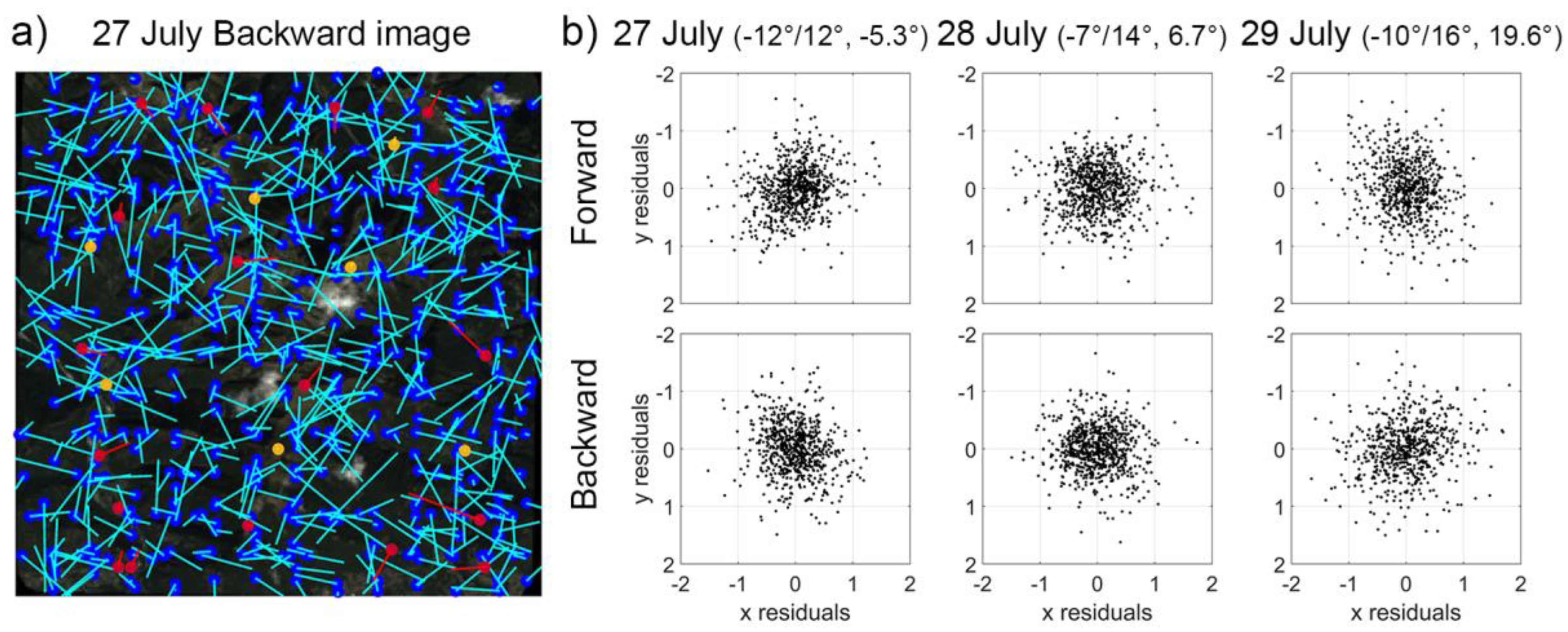
Tot (30)	0.69	0.64	0.82	0.14	0.20	0.27

). The application of the LSM transformation led to a lower RMSE in the Z-direction, which ranges between 0.14 m and 0.27 m. The worst result is shown by the DSM derived from the stereo pair with the largest angle of convergence and across-track angle. The vertical accuracy of Pléiades DSMs over the entire scene was assessed by calculating the distribution of ∆H using the reference ALS dataset i.e., the ALS DTM for the stable areas, and the ALS CHM for the forested areas. Figure 9 allows for a visual comparison of the Pléiades nDSMs for each stereo scene before and after LSM, together with the ALS nDSM, and the orthophoto. Compared to the ALS nDSM, the spatial distribution of the Pléiades nDSMs over stable areas appears clustered before LSM and more homogeneous after LSM. The spatial pattern observed in the Pléiades nDSM suggests a tilt of around ±1 m in north-east/south-west direction between the Pléiades DSM and the ALS DTM, which, however, was significantly reduced by applying a full LSM transformation.

According to the histograms of Pléiades nDSMs in stable areas and ∆H (in forest areas) (Figure 10), the improvement of the accuracy of the CHMs due to LSM is not as significant as in the stable areas, where a considerable reduction of dispersion around zero is visible.

The statistics and the box plots of each stereo pair confirm this observation. Overall, after LSM, nDSM heights in stable areas have a median of almost zero, with a σ_MAD below 0.50 m, whereas CHM errors show a considerably higher dispersion, with a σ_MAD around 4 m (

Table 7. nDSM heights in stable areas and CHM errors (∆H) before and after LSM.

	Before LSM (m)				After LSM (m)
nDSM Stable Areas	Mean	Std	Median	σMAD	Mean	Std	Median	σMAD
27 July (−12°/12°, −5.3°)	0.23	0.63	−0.23	0.48	0.00	0.29	−0.01	0.29
28 July (−7°/14°, 6.7°)	−0.05	0.64	−0.19	0.60	0.14	0.34	−0.03	0.36
29 July (−10°/16°, 19.6°)	−0.05	1.35	−0.14	0.71	0.11	1.23	−0.04	0.42
∆H
27 July (−12°/12°, −5.3°)	0.66	6.11	−0.21	3.85	0.67	6.08	−0.32	3.79
28 July (−7°/14°, 6.7°)	0.57	6.29	−0.17	3.89	0.54	6.28	−0.29	3.85
29 July (−10°/16°, 19.6°)	1.15	6.54	0.20	4.14	1.03	6.49	−0.04	4.07

).

In order to investigate the correlation between the accuracy of the Pléiades CHMs and the reference canopy height, the latter was divided into three height classes, and CHM cells with high variation, i.e., larger than 5.0 m standard deviation within 20 m moving window were excluded (Figure 11a). For all stereo pairs, the CHM errors for tree heights greater than 10 m displays negative median values ranging from −0.58 m to −0.82 m. This can be explained by the tree growth during the two years gap between the Pléiades and ALS data capture. Conversely, the accuracy of the Pléiades CHMs for tree heights below 10 m shows overall positive differences and a considerably higher dispersion for the tree heights smaller than 5 m (Figure 11b). Those trees occupied about 10% of the entire forest area and they are mainly distributed within managed forests areas, as shown in the spatial distribution of the ALS CHM grouped by the three height classes. For this study area, the effect of slope on the accuracy of the Pléiades CHMs cannot be assessed since less than 1% of it reveals a slope greater than 50°.

4.2.2. Accuracy Assessment of the VHR CHMs for the Selected Areas

The quality of the Pléiades CHMs varies according to forest density and forest height. A detailed investigation on the Pléiades CHMs for the two selected areas shows that Pléiades CHMs provided comparable results to the ALS data for a homogenous forest canopy (Figure 12a). Conversely, distinct canopy height patterns that can be seen in the ALS canopy height map cannot be discerned in the Pléiades map where the tree crowns are significantly wider and less defined (Figure 12b). It is worth noting that those differences in the canopy gap characteristics can be attributed to forest management activities, but most likely to the severe freezing rain event that hit Slovenian forests in 2014, damaging 40% forest areas throughout the country [37]. Indeed, the orthophoto acquired simultaneously to ALS data (2015) shows larger canopy gaps than those visible in the Pleiades orthophoto (2013) (Figure 12c).

These qualitative results are confirmed by the distribution of Pleiades CHM height errors, where a clear correlation exists with low forest heights (Figure 13b, area 2). Moreover, the trend also demonstrates that young forest (height < 5 m), which is typically underestimated by image matching [23], is completely missing in the Pleiades results, validating the differences in forest structure at the points in time of Pléiades and ALS data capture. The larger across-track angle shows a wider error dispersion for both areas i.e., forest types.

5. Discussion

This work focuses on analysing the accuracy of Pléiades DSMs over forest mountain regions in order to identify the optimal acquisition planning in terms of stereo or tri-stereo data and incidence angle along- and across-track. Tri-stereo (FNB) images were requested in 2017 over Ticino forest area in Switzerland. The angle of convergence of the forward-backward (FB) images was about 12°, with an average across track-angle of −5°. The three stereo pairs with different across- and along-track angles were acquired in 2013 over the same area in Ljubljana (Slovenia), one day apart from each other. Those images had an angle of convergence of about 24°, 22°, and 27°, respectively, with about −5°, +6° and +20° in across-track direction.

In this study, we focus on the reconstruction of the surface height from pan-sharpened Pléiades images. As reported by Reference [26], if only tree heights are of interest, there is a limited reimbursement of also acquiring and processing spectral and textural data, because multispectral and colour information typically does not contribute to the matching performance [38]. Therefore, in this work, the fourth band was only exploited to generate the NDVI map which was used to derive the tree mask for the Ticino study area and for removing the lake and river surfaces from the stable area mask. The surface covered by clouds was excluded from the analyses in post-processing based on the nDSM.

Processing in Inpho Match-T is highly automated. It requires only limited information to be entered by users, consisting of manually observing GCPs in the images, checking the residuals of tie points to remove blunders, and setting some parameters for the dense point cloud computation e.g., the type of filtering and the spatial resolution (in our work, one point per pixel). The GCPs were employed to achieve sub-meter accuracy. A high number of GCPs improves the accuracy, but no significant improvement can be reached by increasing the number of GCPs from 10 to 40 [39,40]. For both study areas we used 18 GCPs to refine the RPC in combination with automatically extracted tie points. For the tie points, we obtained a precision of better than 0.3 pixels for the tri-stereo images in Ticino and around 0.5 pixels for the three stereo images in Ljubljana. For both study areas, there is a good agreement between the horizontal RMSE of the adjusted coordinates of the GCPs and the CPs on the ground, but high discrepancies can be found in the vertical direction, where the RMSE of the CPs is about 1.0 m (Ticino) and 0.80 m (Ljubljana) in comparison to one decimetre of the GCPs. Because the GCPs were used within the bundle adjustment, only the CPs residuals represent external accuracy. Indeed, this result is validated by the vertical RMSE of the DSM at the GCPs and CPs, which is in total about 0.90 m and 0.70 m for Ticino and Ljubljana, respectively. For the area of Ticino, the vertical DSM RMSE of the CPs is almost twice as large as the one of the GCPs, which suggests a sub-optimal distribution of the GCPs. However, the large forest coverage and the steep terrain limited the selection of GCPs and CPs within this area.

To generate DSMs from dense point clouds, a moving plane interpolation was chosen that consider all the points within a 3 m search radius. This approach was found to be the optimal compromise between minimizing the number of void pixels, preservation of detail, and noise filtering. Considering that the vertical accuracy of photogrammetric DSMs largely depends on the target land cover [11], we assessed the global accuracy of Pléiades DSMs separately for stable areas and for forest areas (CHM) by comparison with the reference data. In stable areas, the Pléiades DSMs elevation errors showed a clustered bias for both study areas. Consequently, the application of an affine transformation estimated by LSM reduced them. However, to derive globally optimal transformation parameters using LSM, the common stable areas in the master and slave surfaces should be homogeneously distributed over the entire scene, which can be hard to achieve in forest mountain areas. Despite this limitation, we demonstrated that for both study areas, LSM improved the geolocation accuracy by removing the clustered error, especially over the flat area of Ljubljana. Moreover, in Ticino, LSM removed the 35 m geolocation error resulting from the original RPCs delivered with the imageries. This accuracy corresponds to the results reported by Reference [39], who estimated an RMSE of the absolute height of the Pléiades DSMs between 35.6 m and 41.9 m when using the original RPCs. Our results indicate that sub-meter geolocation accuracy can be achieved without the time-consuming measurement of GCPs by applying an LSM transformation, if a high-resolution DTM and stable areas are available. In Ticino, some clustered errors were still present after LSM, likely due to the low quality of the reference DTM, which showed abrupt terrain discontinuities. This is confirmed by similar distributions of the nDSMs in stable areas for Pléiades (σ_MAD = 0.82 (FB)) and aerial image matching (σ_MAD = 0.80), where the same DTM was used for normalisation. The application of LSM in Ljubljana significantly removed the tilt effect in the flat stable areas: For the images of 29 July, 74% of the cells fell in the range ±1 m before LSM, whereas the percentage increased to 92% after LSM. The improvement due to LSM of the Pléiades DSM accuracies in forest areas is not as significant as in stable areas. If we quantify this improvement as the percentage of Pléiades DSM cells with height errors within the range of ±1 m, then LSM increases the accuracy by 5 and 4 percentage points for Ticino and Ljubljana, respectively. However, note that in both study areas there is a considerable time gap between the acquisition of the reference data and the Pléiades image.

After LSM, the vertical error distribution of the Pléiades CHMs in Ticino and Ljubljana show good agreement in terms of their median, ranging between 0.02 m (FB) and −0.20 m (NB) for Ticino and between −0.04 m and −0.32 m for Ljubljana. In contrast, their dispersions differ significantly, with a σ_MAD of about 4 m for Ljubljana, as opposed to 2 m for Ticino. This larger dispersion of the error distribution can be attributed to the different forest types and managements of the two study areas. In Ticino, the forest areas were more homogeneous, containing mainly adult trees (87%, >10 m) in broadleaf forest. The height of lower trees was generally overestimated by Pléiades image matching, contrary to the conclusion of Reference [26]. However, in our study, this overestimation can be attributed to tree growth between the time of aerial (2015) and Pléiades (2017) images acquisitions. However, in Ljubljana, only 76% of the canopy cover revealed heights greater than 10 m, and it consists of managed forests, several vegetated urban areas, and single trees in flat areas. Tree growth between the Pléiades (2013) and ALS (2015) data acquisitions can explain the negative differences between Pléiades and ALS CHMs for tree heights greater than 10 m. Younger trees were significantly overestimated by Pleiades CHMs in comparison to ALS. However, note that between these two data acquisitions, the Slovenian forests were hit by a strong ice storm, which caused severe damage. Consequently, many of the canopy gaps formed during this event and the younger trees due to forest regeneration were not yet present at the time of the Pléiades image. This was confirmed by visual comparison of a Pléiades orthophoto and an aerial one acquired at the time of ALS data acquisition. An additional aspect to consider in the comparison of the results for the two study areas is the different kinds of data used to compute the reference DSMs: ALS in Ljubljana versus aerial images in Ticino. Hence, two image sensors (with GSDs of 0.50 m for the aerial and of 0.70 m for the Pleiades images) were compared, which have similar issues concerning gap detection, because the same point has to be visible in at least two images. Hence, accurate CHM reconstruction in mountain areas remains difficult due to strong elevation contrast between trees and the surrounding ground, which results in occlusions. Therefore, we confirm that the ability to accurately measure points between trees heavily depends on the GSD, the base length of stereo images, dominating tree heights and the density of the forest [41]. The analysis of the height profiles confirms that the Pléiades DSMs follow well the aerial DSM (Figure 7) and the ALS DSM (Figure 12c) for homogenous canopy cover and adult trees, but overestimates the height between single trees close to each other and within canopy gaps. This result matches the expectation that stereo-photogrammetry reconstructions yield a relatively smooth surface in which height discontinuity between trees and their surrounding are represented by gradual changes [39,42]. The median of Pléiades CHM errors is not influenced by slope, but a rapid increase of its dispersion was observed for steep areas in Ticino (>60°).

When analysing the quality of Pléiades DSMs regarding the acquisition mode in Ticino, i.e., tri-stereo vs. stereo, we observed in a profile (Figure 7) that the nadir image increases completeness, reducing the data void left out by FB matching in steep forest areas, because of fewer occlusions, and larger image similarity. Anyway, the small angle of convergence (12°) of the FB stereo pair resulted in small unreconstructed areas only that were mostly filled by DSM interpolation. The study shows a limitation of the used software in the dense matching of from tristereo images: The resulting FNB dense point cloud is simply a subset of the two-nadir stereo (FN and NB) point clouds, without any contribution of the FB stereo pair. FB provided the highest accuracy in comparison to the tri-stereo and the two nadir stereo pairs, albeit differences are rather small. Among the two nadir stereo pairs, FN had the smaller angle of convergence, and it provided the worst results, as expected. The reached accuracy of the height model based on all three images (i.e., FN-NB-FB) is slightly better than for FB, as also observed by Reference [42]. Selecting the locally best of the three stereo results (i.e., with minimum local height error) yields an improved model. This selection is straightforward when having reference data at hand that was acquired at the same time as the satellite imagery. Without reference data, however, according selection criteria still remain an open question.

Incidence angles, both across- and along-track, affect DSM accuracy, although our results showed only moderate differences, especially within forest areas. When comparing the accuracies of the study areas, we observed that the larger angle of convergence (>24° of Ljubljana versus 12° in Ticino) provided a σ_MAD in stable areas that was two times smaller. However, this might also be attributed to the more mountainous topography in Ticino and the more homogeneous distribution of the GCPs in Ljubljana. Nevertheless, the median values of the nDSMs in stable areas is close to zero for both study areas, which suggests that a narrow angle of convergence doesn’t constitute a major limiting factor for the quality of the Pléiades DSMs [39]. By contrast, based on the assumption that a wider angle of convergence (>15°) would help to enhance the accuracy of the measured heights [15,43], our results suggest that a wider across-track angle (20°) has a negative impact on the vertical accuracy of the DSM. Furthermore, the error dispersion is more affected by steep terrain than by small across-track angles (±6°).

6. Conclusions

Pléiades satellite images compared to other VHR sensors have the main advantages of a great agility, daily revisit capability, smaller time intervals between the image acquisition and the possibility to acquire a nadir-looking view. Considering these characteristics and if a digital terrain model (DTM) is available, the system offers a great potential for providing a high spatial resolution canopy height model (CHM), which can be used for supporting forest inventory and monitoring programs at the regional and national level. Therefore, to take this system into consideration, an important challenge is to understand the accuracy of the derived products. Specifically, since the acquisition mode (Tri-stereo/stereo) and the incidence angles can be planned for the new Pléiades images acquisitions, this work wants to answer the following two questions: (1) what is the benefit of using tri-stereo images and (2) what is the impact of different incidence angles along- and across-track on the image matching performance and on the accuracy of the DSM. In order to derive the height above the ground (i.e., the nDSM), available DTM was subtracted from the DSMs. The image orientation implied the use of GCPs and tie points to refine the RPC. However, in order to remove systematic errors on the generated DSMs, an affine transformation (LSM) was successfully applied to the dense point cloud. We demonstrated that by applying an LSM transformation sub-meter geolocation accuracy without the time-consuming GCPs measurements could be achieved.

Our results suggest that the differences between tri-stereo and stereo matching are rather small and the stereo forward-backward canopy height showed slightly higher accuracies than the tristereo results and the two nadir stereo pairs. In terms of completeness, the nadir image can minimize the issues of stereo matching in steep forest areas, but the adopted interpolation method and the narrow angle of convergence of the forward-backward pair yielded to small unreconstructed areas. Both incidence angles, across- and along-track are important parameters for determining DSM accuracy of a stereo pair, although our results do not show dramatic differences. However, a large across-track angle (19°) reduces the quality of Pléiades CHMs/nDSMs.

References

1. Immitzer, M.; Stepper, C.; Böck, S.; Straub, C.; Atzberger, C. Use of WorldView-2 stereo imagery and National Forest Inventory data for wall-to-wall mapping of growing stock. For. Ecol. Manag. 2016, 359, 232–246. [Google Scholar] [CrossRef]
2. Lim, K.; Treitz, P.; Wulder, M.; St-Onge, B.; Flood, M. LiDAR remote sensing of forest structure. Prog. Phys. Geogr. 2003, 27, 88–106. [Google Scholar] [CrossRef]
3. Latifi, H.; Nothdurft, A.; Koch, B. Non-parametric prediction and mapping of standing timber volume and biomass in a temperate forest: Applications of multiple optical/LiDAR-derived predictors. Forestry 2010, 83, 395–407. [Google Scholar] [CrossRef]
4. Vastaranta, M.; Wulder, M.A.; White, J.C.; Pekkarinen, A.; Tuominen, S.; Ginzler, C.; Hyyppä, H. Airborne laser scanning and digital stereo imagery measures of forest structure: Comparative results and implications to forest mapping and inventory update. Can. J. Remote Sens. 2013, 39, 382–395. [Google Scholar] [CrossRef]
5. Leberl, F.; Irschara, A.; Pock, T.; Meixner, P.; Gruber, M.; Scholz, S.; Wiechert, A. Point clouds. Photogramm. Eng. Remote Sens. 2010, 76, 1123–1134. [Google Scholar] [CrossRef]
6. Kayitakire, F.; Hamel, C.; Defourny, P. Retrieving forest structure variables based on image texture analysis and Ikonos-2 imagery. Remote Sens. Environ. 2006, 102, 390–401. [Google Scholar] [CrossRef]
7. Uddin, K.; Gilani, H.; Murthy, M.S.R.; Kotru, R.; Qamer, F.M. Forest condition monitoring using very-high-resolution satellite imagery in a remote mountain watershed in Nepal. Mt. Res. Dev. 2015, 35, 264–277. [Google Scholar] [CrossRef]
8. Shamsoddini, A.; Trinder, J.C.; Turner, R. Pine plantation structure mapping usingWorldView-2 multispectral image. Int. J. Remote Sens. 2013, 34, 3986–4007. [Google Scholar] [CrossRef]
9. Persson, H.J.; Perko, R. Assessment of boreal forest height from WorldView-2 satellite stereo images. Remote Sens. Lett. 2016, 7, 1150–1159. [Google Scholar] [CrossRef] [Green Version]
10. Song, C.; Dickinson, M.B.; Su, L.; Zhang, S.; Yaussey, D. Estimating Average Tree Crown Size Using Spatial Information from Ikonos and QuickBird Images: Across-sensor and Across-Site Comparisons. Remote Sens. Environ. 2010, 114, 1099–1107. [Google Scholar] [CrossRef]
11. Hobi, M.L.; Ginzler, C. Accuracy assessment of digital surface models based on WorldView-2 and ADS80 stereo remote sensing data. Sensors 2012, 12, 6347–6368. [Google Scholar] [CrossRef] [PubMed]
12. Hobi, M.L.; Ginzler, C.; Commarmot, B.; Bugmann, H. Gap pattern of the largest primeval beech forest of Europe revealed by remote sensing. Ecosphere 2015, 6, 1–15. [Google Scholar] [CrossRef]
13. Bagnardi, M.; González, P.J.; Hooper, A. High-resolution digital elevation model from tri-stereo Pleiades-1 satellite imagery for lava flow volume estimates at Fogo Volcano. Geophys. Res. Lett. 2016, 43, 6267–6275. [Google Scholar] [CrossRef] [Green Version]
14. De Lussy, F.; Greslou, D.; Dechoz, C.; Amberg, V.; Delvit, J.M.; Lebegue, L.; Blanchet, G.; Fourest, S. Pleiades HR in flight geometrical calibration: Location and mapping of the focal plane, ISPRS International Archives of the Photogrammetry. Remote Sens. Spat. Inf. Sci. 2012, 39, 519–523. [Google Scholar]
15. Poli, D.; Caravaggi, I. 3D modeling of large urban areas with stereo VHR satellite imagery: Lessons learned. Nat. Hazards 2013, 68, 53–78. [Google Scholar] [CrossRef]
16. Perko, R.; Raggam, H.; Gutjahr, K.; Schardt, M. Assessment of the mapping potential of Pléiades stereo and triplet data. ISPRS Ann. Photogramm. Remote Sens. Spat. Inf. Sci. 2014, 2, 103. [Google Scholar] [CrossRef]
17. Jacobsen, K.; Topan, H. DEM generation with short base length Pleiades triplet. Int. Arch. Photogramm. Remote Sens. Spat. Inf. Sci.-ISPRS Arch. 2015, 40, 81–86. [Google Scholar] [CrossRef]
18. Poli, D.; Remondino, F.; Angiuli, E.; Agugiaro, G. Radiometric and geometric evaluation of GeoEye-1, WorldView-2 and Pléiades-1A stereo images for 3D information extraction. ISPRS J. Photogramm. Remote Sens. 2015, 100, 35–47. [Google Scholar] [CrossRef]
19. Panagiotakis, E.; Chrysoulakis, N.; Charalampopoulou, V.; Poursanidis, D. Validation of Pleiades Tri-Stereo DSM in Urban Areas. ISPRS Int. J. Geo-Inf. 2018, 7, 118. [Google Scholar] [CrossRef]
20. Eisank, C.; Rieg, L.; Klug, C.; Kleindienst, H.; Sailer, R. Semi-Global Matching of Pléiades tri-stereo imagery to generate detailed digital topography for high-alpine regions. J. Geogr. Inf. Sci. 2015, 2015, 168–177. [Google Scholar] [CrossRef]
21. Himmelreich, L.C.; Ladner, M.; Heller, A. Pléiades Tri-Stereo-Bilder im Hochgebirge–eine Parameterstudie mit PCI Geomatics. Agit–J. für Angewandte Geoinformatik 2017, 3, 153–162. [Google Scholar] [CrossRef]
22. Himmelreich, L. DHM Ableitungen aus Pléiades Tri-Stereo Satellitenbildern im Hochgebirge. Digitale Höhenmodelle Verschiedener Softwareprodukte im Vergleich zu ALS Daten. Master Thesis, University of Innsbruck, Innsbruck, Austria, July 2017. [Google Scholar]
23. Zhou, Y.; Parsons, B.; Elliott, J.R.; Barisin, I.; Walker, R.T. Assessing the ability of Pleiades stereo imagery to determine height changes in earthquakes: A case study for the El Mayor-Cucapah epicentral area. J. Geophys. Res. Solid Earth 2015, 120, 8793–8808. [Google Scholar] [CrossRef]
24. Beguet, B.; Guyon, D.; Boukir, S.; Chehata, N. Automated retrieval of forest structure variables based on multi-scale texture analysis of VHR satellite imagery. ISPRS J. Photogramm. Remote Sens. 2014, 96, 164–178. [Google Scholar] [CrossRef]
25. Trisakti, B. Vegetation type classification and vegetation cover percentage estimation in urban green zone using pleiades imagery. In IOP Conference Series: Earth and Environmental Science; IOP Publishing: Bristol, UK, 2017; Volume 54. [Google Scholar]
26. Persson, H. Estimation of Boreal Forest Attributes from Very High Resolution Pléiades Data. Remote Sens. 2016, 8, 736. [Google Scholar] [CrossRef]
27. Maack, J.; Kattenborn, T.; Fassnacht, F.E.; Enßle, F.; Hernández, J.; Corvalán, P.; Koch, B. Modeling forest biomass using Very-High-Resolution data—Combining textural, spectral and photogrammetric predictors derived from spaceborne stereo images. Eur. J. Remote Sens. 2015, 48, 245–261. [Google Scholar] [CrossRef]
28. Abdollahnejad, A.; Panagiotidis, D.; Surový, P. Estimation and Extrapolation of Tree Parameters Using Spectral Correlation between UAV and Pléiades Data. Forests 2018, 9, 85. [Google Scholar] [CrossRef]
29. Akbari, H.; Kalbi, S. Determining Pleiades satellite data capability for tree diversity modeling. iForest-Biogeosci. For. 2016, 10, 348. [Google Scholar] [CrossRef]
30. Pearse, G.D.; Dash, J.P.; Persson, H.J.; Watt, M.S. Comparison of high-density LiDAR and satellite photogrammetry for forest inventory. ISPRS J. Photogramm. Remote Sens. 2018, 142, 257–267. [Google Scholar] [CrossRef]
31. Ginzler, C. Vegetation Height Model NFI. Natl. For. Inventory (NFI) 2018. [Google Scholar] [CrossRef]
32. Pfeifer, N.; Mandlburger, G.; Otepka, J.; Karel, W. OPALS—A framework for Airborne Laser Scanning data analysis. Comput. Environ. Urban Syst. 2014, 45, 125–136. [Google Scholar] [CrossRef]
33. Fraser, C.S.; Dial, G.; Grodecki, J. Sensor orientation via RPCs. ISPRS J. Photogramm. Remote Sens. 2006, 60, 182–194. [Google Scholar] [CrossRef]
34. Astrium. Pléiades Imagery User Guide V 2.0.; Astrium: Toulouse, France, 2012. [Google Scholar]
35. Heuchel, T.; Köstli, A.; Lemaire, C.; Wild, D. Towards a next level of quality DSM/DTM extraction with Match-T. Proc. Photogramm. Week 2011, 11, 197–202. [Google Scholar]
36. Ressl, C.; Mandlburger, G.; Pfeifer, N. Investigating Adjustment of Airborne Laser Scanning Strips without Usage of GNSS/IMU Trajectory Data. In Proceedings of the ISPRS Workshop Laserscanning 09, Paris, France, 1–2 September 2009; Volume XXXVIII, pp. 195–200. [Google Scholar]
37. Nagel, T.A.; Firm, D.; Rozenbergar, D.; Kobal, M. Patterns and drivers of ice storm damage in temperate forests of Central Europe. Eur. J. For. Res. 2016, 135, 519–530. [Google Scholar] [CrossRef]
38. Bleyer, M.; Chambon, S. Does color really help in dense stereo matching. In Proceedings of the International Symposium 3D Data Processing, Visualization and Transmission, 3DPVT 2010, Paris, France, 17–20 May 2010; pp. 1–8. [Google Scholar]
39. Stumpf, A.; Malet, J.P.; Allemand, P.; Ulrich, P. Surface reconstruction and landslide displacement measurements with Pléiades satellite images. ISPRS J. Photogramm. Remote Sens. 2014, 95, 1–12. [Google Scholar] [CrossRef]
40. Topan, H.; Cam, A.; Özendi, M.; Oruç, M.; Jacobsen, K.; Taşkanat, T. Pléiades project: Assessment of georeferencing accuracy, image quality, pansharpening performence and DSM/DTM quality. Int. Arch. Photogramm. Remote Sens. Spat. Inf. Sci.-ISPRS Arch. 2016, 41, 503–510. [Google Scholar] [CrossRef]
41. Zarco-Tejada, P.J.; Diaz-Varela, R.; Angileri, V.; Loudjani, P. Tree height quantification using very high resolution imagery acquired from an unmanned aerial vehicle (UAV) and automatic 3D photo-reconstruction methods. Eur. J. Agron. 2014, 55, 89–99. [Google Scholar] [CrossRef] [Green Version]
42. White, J.C.; Tompalski, P.; Coops, N.C.; Wulder, M.A. Comparison of airborne laser scanning and digital stereo imagery for characterizing forest canopy gaps in coastal temperate rainforests. Remote Sens. Environ. 2018, 208, 1–14. [Google Scholar] [CrossRef]
43. Bernard, M.; Decluseau, D.; Gabet, L.; Nonin, P. 3D capabilities of Pleiades satellite. International archives of the photogrammetry. Remote Sens. Spat. Inf. Sci. 2012, 39, 553–557. [Google Scholar]
Figure 1. Study areas and imaging geometries of the Pléiades data sets (Google Earth preview of the footprints and the satellite’s position).
Remotesensing 10 01542 g001
Figure 2. General workflow to generate the nDSMs from Pléiades images.
Remotesensing 10 01542 g002
Figure 3. For (a) the Ticino and (b) the Ljubljana study areas, left: the 3D point cloud. Centre: the orthophoto generated from the 4-bands Pléiades images, visualised as true colour RGB, and overlaid with the GCPs (red circles) and CPs (orange circles). The yellow rectangles represent the common regions of interest for all scene combinations. Right: the colour coded, reconstructed DSMs. The blue squares are the 500 × 500 m selected areas.
Remotesensing 10 01542 g003
Figure 4. nDSM statistics for stable areas, with results before (top) and after (bottom) LSM. (Left) colour coding of the Pléiades (FNB) and aerial nDSMs (non-stable areas shown in white). (Right) distribution of nDSM heights for the aerial images, and for the Pléiades tri-stereo and all stereo pairs.
Remotesensing 10 01542 g004
Figure 5. Height differences (ΔH) between Pléiades and aerial CHMs before (top) and after (bottom) LSM. (Left) spatial distribution for FNB as colour coding (areas outside forest mask shown in white). Centre: distributions of ΔH for tri-stereo and all stereo pairs as histograms. (Right) the same distributions shown as box plots.
Remotesensing 10 01542 g005
Figure 6. Box plots of the distributions of ∆H after LSM for different classes of (a) reference canopy height, and (b) terrain slope. Respective cell counts are plotted in grey and refer to the right axes.
Remotesensing 10 01542 g006
Figure 7. Profiles of 1 m width of the tri-stereo and stereo Pléiades point clouds (top) and of the Pléiades nDSMs for each stereo pair in comparison to the reference aerial nDSM (bottom). The red line in the orthophoto indicates the position of the profiles.
Remotesensing 10 01542 g007
Figure 8. (a) Histograms of the absolute height errors (Abs∆H) for each Pléiades CHM (MinAbs∆H i.e., optimal selection from stereo DSMs, NB, FN, FB, and FB-NB-FN), and (b) the spatial distribution of the stereo pairs with locally minimum absolute differences (MinAbs∆H).
Remotesensing 10 01542 g008
Figure 9. The spatial distribution of the nDSMs of ALS (left, top) and each Pléiades stereo scene before (right, top) and after (righ, bottom) LSM. At the (left, bottom), the orthophoto derived from the forward Pléiades image of 27 July is shown.
Remotesensing 10 01542 g009
Figure 10. Distribution of nDSM heights in stable areas (left) and CHM errors (∆H) before (right, top) and after (right, bottom) LSM for each stereo pair.
Remotesensing 10 01542 g010
Figure 11. (a) The spatial distribution of the three reference CHM tree height classes, disregarding areas with large height variation. Distributions of the CHM error (∆H) for each stereo pair after LSM grouped by (b) tree height class and (c) terrain slope.
Remotesensing 10 01542 g011
Figure 12. For the selected (a) area 1 and (b) area 2, the reference CHM (left), the Pléiades CHMs for each stereo pair (centre), and the orthophoto generated from the four bands Pléiades image (right). The dashed black line in ((a), left) indicates the position of the profiles of 1 m width of reference and Pléiades CHMs shown on the left of (c). On the right of (c), the aerial orthophoto for area 2 that was acquired simultaneously to the reference data.
Remotesensing 10 01542 g012
Figure 13. 2D histograms of Pléiades CHM errors and reference CHM for the selected (a) area 1 and (b) area 2, and each stereo pair (left, centre, right).
Remotesensing 10 01542 g013