Improvement of Clay and Sand Quantification Based on a Novel Approach with a Focus on Multispectral Satellite Images

Abstract

Soil mapping demands large-scale surveys that are costly and time consuming. It is necessary to identify strategies with reduced costs to obtain detailed information for soil mapping. We aimed to compare multispectral satellite image and relief parameters for the quantification and mapping of clay and sand contents. The Temporal Synthetic Spectral (TESS) reflectance and Synthetic Soil Image (SYSI) approaches were used to identify and characterize texture spectral signatures at the image level. Soil samples were collected (0–20 cm depth, 919 points) from an area of 14,614 km² in Brazil for reference and model calibration. We compared different prediction approaches: (a) TESS and SYSI; (b) Relief-Derived Covariates (RDC); and (c) SYSI plus RDC. The TESS method produced highly similar behavior to the laboratory convolved data. The sandy textural class showed a greater increase in average spectral reflectance from Band 1 to 7 compared with the clayey class. The prediction using SYSI produced a better result for clay (R² = 0.83; RMSE = 65.0 g kg⁻¹) and sand (R² = 0.86; RMSE = 79.9 g kg⁻¹). Multispectral satellite images were more stable for the identification of soil properties than relief parameters.

1. Introduction

The characteristics of the topsoil layer are important because they provide fundamental information for food production. Soil is composed of physical, chemical, mineralogical, and organic compounds, plus water and air, and these properties have been degraded in many agricultural regions through poor management actions [1]. An important soil property related to physical structure is the particle size distribution, which is divided into three main fractions: clay (<0.002 mm), silt (0.002–0.02 mm), and sand (>0.02 mm). The clay fraction influences several important processes, such as water retention and infiltration, nutrient dynamics, and root development. Moreover, particle size is also directly related to soil compaction, plasticity, consistency, mechanical resistance, air capacity, pollutants, and herbicide interactions [2].

Pedometric soil mapping uses quantitative information obtained by different methods, ranging from conventional cartographical surveys (elevation models from which terrain attributes can be derived) to Proximal Sensing (PS) and Remote Sensing (RS). Ben-Dor and Banin [3] described the so-called NIRA (Near-Infrared Analysis), which has been the basis for attribute quantification by spectroscopy. Several other studies have confirmed the potential of PS levels for quantifying soil attributes, such as clay content [4,5] and textural classes [6]. Based on this strong spectroscopy background, research has moved towards remote satellite information, as in Coleman et al. [7]. More recently, Mouazen et al. [8] and Morellos et al. [9], in order to offer operational solutions for systematic coverage of fields, applied on-line sensors at accuracies comparable to laboratory analyses.

Pedologists, pedometricians, and environmental analysts often use continuous information from the landscape in a flexible and direct manner to describe soil variability through space and time. In fact, McBratney et al. [10] describe soil variability as “continuous” and without rigid limits. Occasional bare soil regions can be identified in fragmented areas, but this is not ideal for a spatially continuous map.

Pedologists currently use imagery to assist in understanding the direction of soil variability for its mapping. This leads soil mappers to use relief information as a basis to map an entire area. At this point, images may be of assistance because they are able to indicate areas with bare soil; however, scientific articles tackling this issue are generally limited to detecting point-based information, while spatially continuous solutions are still lacking.

There is a gap concerning how to use RS to assist digital soil mapping. Some recent publications in this area have used the relationship between soil particle size, landscape topography, and spectral reflectance [11], while other studies have targeted the prediction of clay content, applying laboratory spectral measurements and satellite multispectral data (

Table 1. Literature review concerning prediction of clay content by laboratory spectral data, satellite multispectral data, and relief-derived covariates.

Source	Sensor 1	R2 Range	Author(s)
Laboratory	UV-VIS-NIR (20–2500 nm)	0.61–0.80	Islam et al. [12]
			Pirie et al. [13]
			Veum et al. [14]
	VIS-NIR-SWIR (350–2500 nm)	0.75–0.91	Wang and Pan [15]
			O’Rourke et al. [16]
			Conforti et al. [17]
			Pinheiro et al. [18]
			Adeline et al. [19]
			Dotto et al. [20]
Satellite	TM	0.44–0.67	Henderson et al. [21]
			Nanni and Demattê [22]
			Fiorio et al. [23]
			Shabou et al. [24]
	ETM+	0.26–0.68	Chagas et al. [25]
			Diek et al. [26]
	Jena-Optronik (RapidEye)	0.24–0.56	Forkuor et al. [27]
	EO-1 ALI (Hyperion)	0.51–0.83	Zhang et al. [28]
			Castaldi et al. [29]
Relief-Derived Covariates	Elevation, Slope, Convergence Index, and Topographic Wetness Index	0.55	Samuel-Rosa et al. [30]
	Relative Elevation and Slope	0.07	Sumfleth and Duttman [31]
	Slope, Plan Convexity, and Upslope Distance	0.51	Odeh et al. [32]

¹ Spectral regions of laboratory sensors: UV: Ultra Violet, VIS: Visible (blue, red, and green), NIR: Near-Infrared, SWIR: Shortwave Infrared. Spectral sensors of satellites: TM: Thematic Mappers, ETM+: Enhanced Thematic Mapper Plus, EO-1 ALI: Earth Observing-1 Advanced Land Imager.

). Regarding the statistical quality of clay prediction, laboratory spectral results have achieved R² values ranging from 0.61 to 0.9 (Table 1). Satellite multispectral sensors achieved lower results, with R² values ranging from 0.26 to 0.83.

Therefore, literature studies have brought us to important points for evaluation towards the usefulness of soil image analysis, as follows: (a) Is there room to increase the prediction of clay content by multispectral sensors, as they have some limitations compared with hyperspectral ones (distance, spectral, and spatial resolution)? (b) An important paradigm supported by many users is that soils cannot be evaluated using images since they are usually covered by vegetation; (c) Relief parameters have been considered to be the best information sources for mapping soil attributes because they are soil formation factors.

Several hypotheses were formulated to address these questions as follows: (1) A Landsat multispectral sensor can quantify clay and sand contents since it has key bands distributed along VIS-NIR-SWIR; (2) Soil spectral libraries can assist in the interpretation and characterization of satellite information; (3) We also expect that a composite of temporal imagery can achieve the best mapping of spatially continuous bare soil data since it will fill the gaps where soil was bare in one period and covered in another; (4) Soil properties are typically determined by classical tacit knowledge, which makes inferences along landforms or by mathematical procedures and interpolation. Spectra from pixels are a direct source of information, and should draw a better picture of clay and sand distribution than reliefs. One technique that can detect even the barest soil over time periods is the Geospatial Soil Sensing System (GEOS3) [33], which will be evaluated in this study. Thus, the main objective of this study is to evaluate multispectral satellite images for clay and sand content quantification and mapping.

2. Materials and Methods

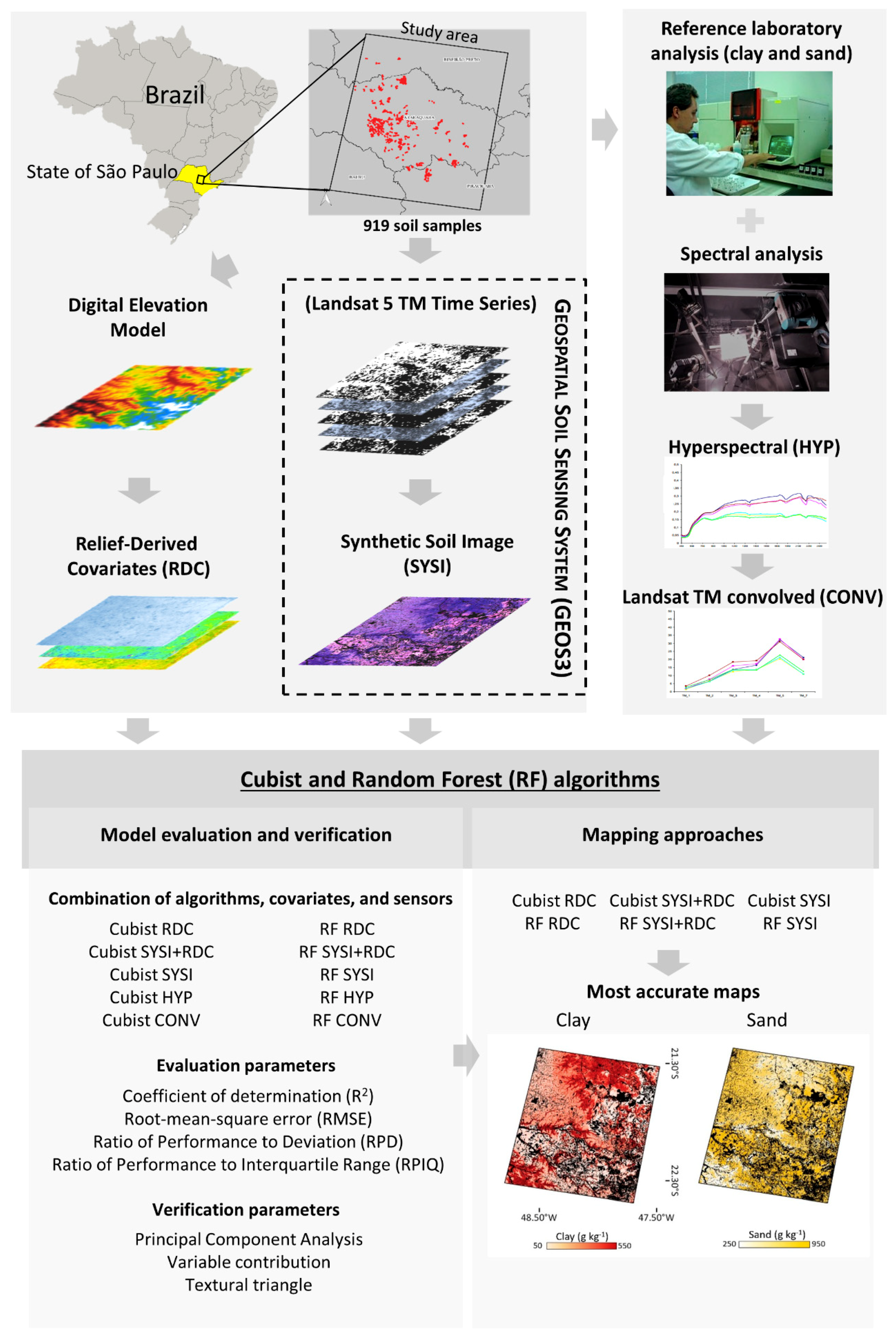
2.1. Study Area

The study area is located in the central region of São Paulo state, Brazil, with a total area of 14,614 km² (Figure 1). The climate in the region is classified as humid subtropical (Cwa) according to the Köppen classification, with dry winters and hot summers [34]. The mean annual precipitation is 1480 mm, while the mean annual maximum and minimum temperatures are 28 °C and 15 °C, respectively. The terrain elevation varies between 400 and 1100 m above sea level. The predominant soils are Ferralsols, Lixisols, Arenosols, and Nitosols, with different particle size distributions [35]. The primary land uses are for sugarcane, silviculture, oranges, and pasture. This area was selected because it is subject to intense agricultural usage and great soil variation, expressing the characteristics of a typical tropical region.

2.2. Field Sampling and Soil Analysis

Soil samples were established in catenas to represent variations of relief and geology using a centimeter-accuracy (RTK) Trimble GPS unit (Figure 1), and were collected at 0–20 cm depth at a total of 919 locations. All soil samples were ground, dried, and sieved (2 mm), and spectral reflectance measurements were taken using a Spectroradiometer FieldSpec 3 sensor (ASD, Boulder, CO, USA) in the 350 to 2500 nm range (Visible, VIS; Near-infrared, NIR; and Shortwave infrared, SWIR) under laboratory conditions. A white Spectralon plate was used as a reference plate with a 50 W halogen lamp positioned at 35 cm from the platform with a zenith angle of 30°. Samples were placed on petri dishes and the sensor was positioned vertically at 8 cm from the platform. The soil samples were also analyzed in the laboratory to determine particle size fractions, following the Pipette method [36]. Spectral reflectance information acquired in the laboratory was also convolved to the Landsat TM bands, assuming a Gaussian response function for the full width at half the maximum spectral response of the sensor [37].

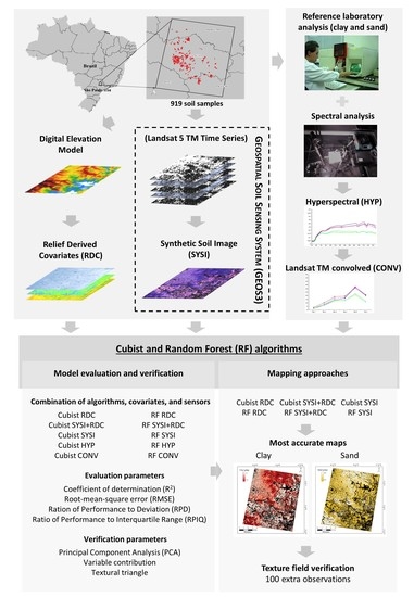
2.3. A Brief Description of the Geospatial Soil Sensing System (GEOS3)

The GEOS3 was developed by Demattê et al. [33], and is defined as a data mining procedure to process multitemporal Landsat 5 TM Time Series. A user can define a time series containing only cloud-free images from the dry season (to avoid moisture interference) and obtain the same from a database containing legacy data [38]. The method to retrieve topsoil reflectance can be summarized as follows. The system uses a time series of atmospherically corrected Landsat 5 TM images transformed into surface reflectance. All images are masked using several approaches, including NDVI and NBR2, among others, and the pixels that are not soil are extracted. Then, all images containing the remaining pixels with bare soil are superimposed, and the system averages the reflectance to produce the median spectral reflectance, resulting in the Temporal Synthetic Spectral (TESS) reflectance. The composite of all TESS values generates a unique spatially continuous image called the Synthetic Soil Image (SYSI). The SYSI is based on the availability of remote sensing spectral reflectance measurements at different times which are used to achieve spatially continuous maps, rather than modelling, interpolating, or inferencing the soil surface.

2.4. Image and Spectral Information

The Landsat data were selected from orbit 220 and path 75, in the period of 1984 to 2011, totaling 151 images. During the time series, most cropping systems were characterized by a period with bare soil. In general, mechanical crop operations are carried out during May and October, matched with the dry season, where the effects of soil moisture can be minimized in the images. In addition, both natural and anthropogenic locations present bare soil, most of which is plowed. The six spectral bands acquired by the sensor are suitable for soil characterization, with measurements in the VIS-NIR-SWIR bands. The atmospherically and geometrically processed higher-level products were acquired from EROS (Earth Resource Observation and Science Center). These products consist of surface reflectance derived through the Landsat Ecosystem Disturbance Adaptive Processing System (LEDAPS). The products are based on Radiative Transfer Modeling performed by the 6S algorithm [39].

GEOS3 was used to construct a single image (SYSI) of the study area (Figure 2a), from which 919 topsoil samples were collected and their laboratory spectra measured. The SYSI indicated that 68% of the pixels were bare soil over the entire study area. More specifically, this corresponded to 92% of the agricultural areas. The spectral signature from the laboratory (convolved to Landsat bands) was compared with the respective spectra from the image (TESS). A morphological evaluation of the spectra was carried out between the sources, as indicated by Demattê et al. [40], considering the intensity and shape. Furthermore, models were constructed to quantify clay and sand content based on spectral reflectance information both from the laboratory and from the SYSI [41]. The values from the raster layers at sampling points were extracted using bilinear interpolation, which uses the four nearest neighbors to find a weighted average for the georeferenced point.

2.5. Preprocessing and Model Calibration

A Digital Elevation Model (DEM) (Figure 2b) derived from Shuttle Radar Topography Mission (SRTM v.3, 30 m) data was used to derive five ancillary terrain variables (elevation, vertical distance to channel network, valley depth, relative slope position, and channel network base level). These five terrain covariates were chosen to represent the variability of the area (

Table 2. Descriptive statistics of the environmental covariates used for clay and sand mapping.

Covariate	Description	Unit	Min	Max	Mean	SD
B1	Band no. 1 from the SYSI [33] with the Landsat 5 TM spectral range 450–520 nm	Reflectance factor	0	0.1	0.05	0.01
B2	Band no. 2 from the SYSI [33] with the Landsat 5 TM spectral range 520–600 nm	Reflectance factor	0	0.16	0.08	0.02
B3	Band no. 3 from the SYSI [33] with the Landsat 5 TM spectral range 630–690 nm	Reflectance factor	0	0.22	0.12	0.03
B4	Band no. 4 from the SYSI [33] with the Landsat 5 TM spectral range 760–900 nm	Reflectance factor	0	0.35	0.18	0.05
B5	Band no. 5 from the SYSI [33] with the Landsat 5 TM spectral range 1550–1750 nm	Reflectance factor	0	0.53	0.22	0.08
B7	Band no. 7 from the SYSI [33] with the Landsat 5 TM spectral range 2080–2350 nm	Reflectance factor	0	0.49	0.21	0.08
DEM	Elevation from the digital elevation model of Shuttle Radar Topography Mission (1 arc second ~ 30 m) with vertical inaccuracy <16 m	m	450	924	615.45	84.58
CNBL	Channel network base level calculated from SAGA GIS version 2.1.2 [44]	m	442.64	883.71	595.75	81.69
RS	Relative slope calculated from SAGA GIS version 2.1.2 [44]	fraction	0	1	0.45	0.33
VD	Valley depth calculated from SAGA GIS version 2.1.2 [44]	m	0	132.98	31.15	27.37
VDTCN	Vertical distance to channel network calculated from SAGA GIS version 2.1.2 [44]	m	0	117.27	19.97	17.19
X	X projected coordinate calculated from SAGA GIS version 2.1.2 [44]	m	127,994.66	213,372.23	163,710.79	19,077.86
Y	Y projected coordinate calculated from SAGA GIS version 2.1.2 [44]	m	7,534,046.16	7,635,498.16	7,576,885.92	21,724.02

SYSI: Synthetic Soil Image; SD: standard deviation.

). According to Moura-Bueno et al. [42], SRTM can represent maps at scales from 1: 25,000 to 1: 50,000. They were generated using the compound terrain analysis function of SAGA GIS.

RDC values and the reflectance from SYSI were extracted at the same locations as the soil samples using bilinear interpolation. The SYSI provided reflectance in the six original Landsat 5 TM bands (VIS-NIR-SWIR): Band (B) 1 (450–520 nm), B2 (520–600 nm), B3 (630–690 nm), B4 (760–900 nm), B5 (1550–1750 nm), and B7 (2080–2350 nm). Then, the 919 georeferenced samples were divided into textural classes for stratified random sampling as follows (g kg⁻¹): very sandy (<100), sandy (100–150), sandy loam (150–250), clayey loam (250–350), clayey (350–600), and very clayey (> 600). Samples were randomly divided into calibration (75%, n = 686) and validation (25%, n = 233) sets. The textural classes are related to the importance of clay and soil management in Brazil, as referenced in Santos et al. [43].

Clay and sand quantification were also carried out using laboratory spectral measurements. The same dataset was used to convolve to Landsat 5 TM bands. These approaches were used to compare data sources and spectral resolutions. Only the SYSI, RDC, and the two combined were used for the topsoil mapping, as these covariates have their spatial representation. The spatial coordinates were also used as covariates, enabling enhanced spatial stratification by the models. Clay and sand predictive models were tested using the Cubist and Random Forest (RF) algorithms. The Cubist algorithm finds the relationships between soil covariates by calculating decision trees and multiple regressions. It was implemented using the Cubist R package ensemble with 15 to 20 committees trying to find the best fit model [45]. RF constructs an ensemble of multiple decision trees (ntree = 1000 and mtry = default), returning their mean prediction. The RF algorithm was implemented using the randomForest R package [46]. The selected models were considered when the Root-Mean-Squared Error (RMSE) was minimized and stabilized in the calibration. The statistical procedures were carried out in the programming language R [47].

2.6. Soil Maps and Validation

Soil clay and sand maps were produced by applying the models using the raster R package [48]. Predictions by Cubist and RF models were made for the pixels containing all the covariates stacked. SYSI had discontinuity gaps (black regions) which generated unmapped areas because they were related to natural forests or other permanent land uses not assessed by GEOS3. The best validated models (lowest RMSE) using the different approaches (SYSI, RDC, and SYSI + RDC) were used to illustrate spatial variations and artifact production between the covariates. Additionally, predictions did not consider possible spatial dependencies for the properties, i.e., using variogram analysis.

The external validation (25% of samples, n = 233) was performed as a comparison between predicted values and results from the reference physical laboratory analysis. The parameters used to evaluate the performance of the models were RMSE, the coefficient of determination (R²), Ratio of Performance to the Interquartile range (RPIQ) [49], and Ratio of Performance to Deviation (RPD). Differences observed in the predicted clay and sand distributions were also described by plotting the model’s outputs in the texture triangle implemented through the soiltexture R package [50].

3. Results and Discussion

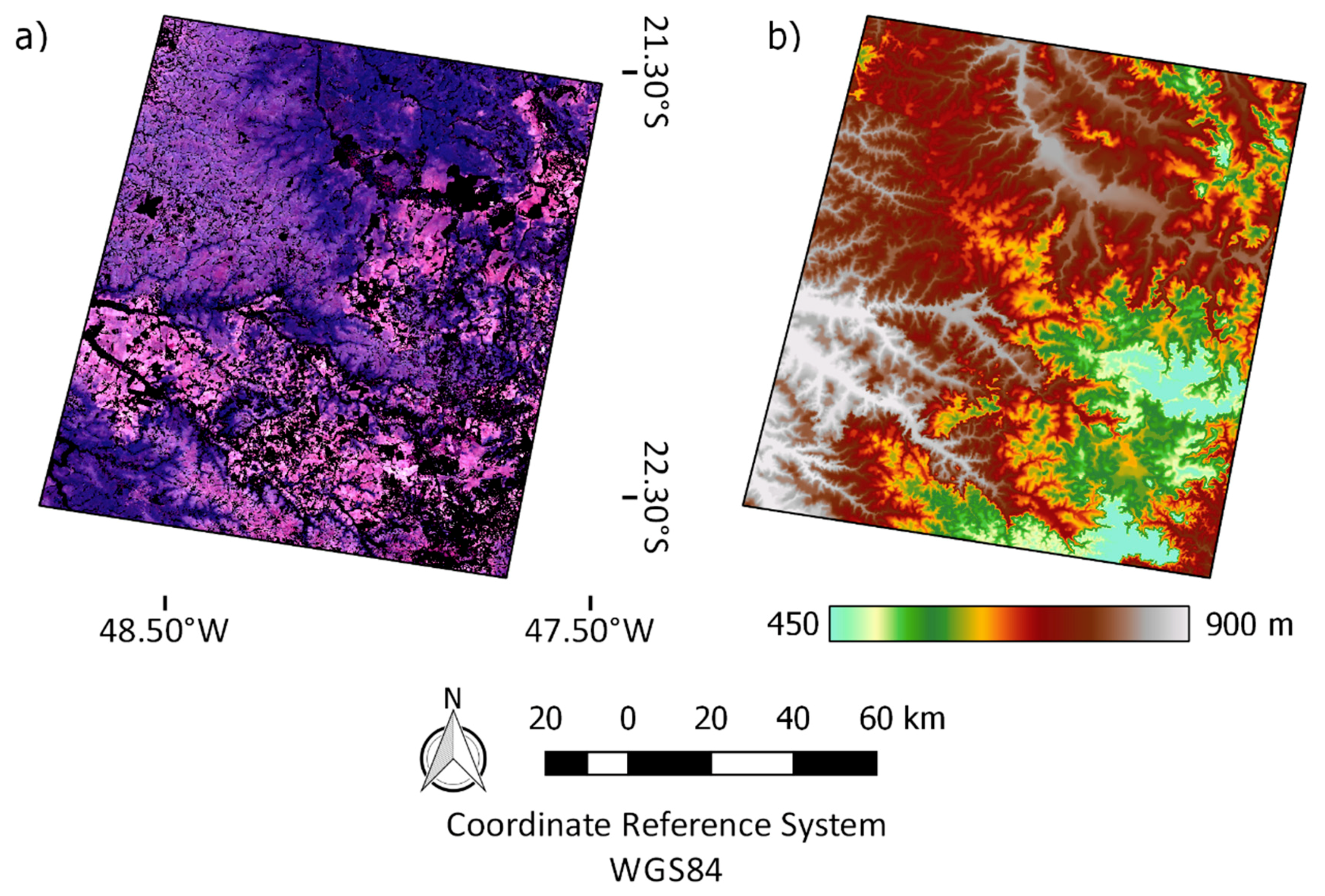
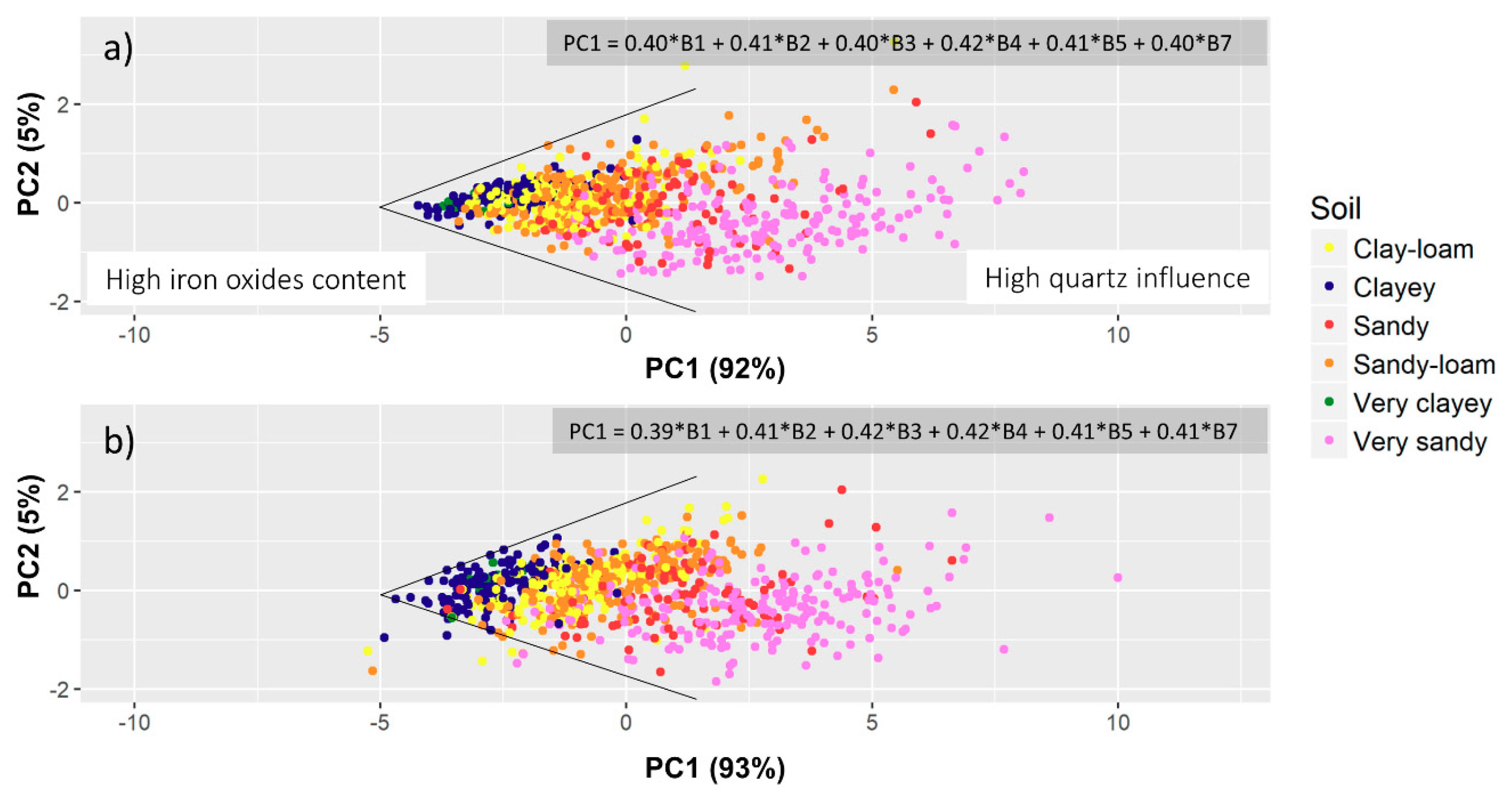
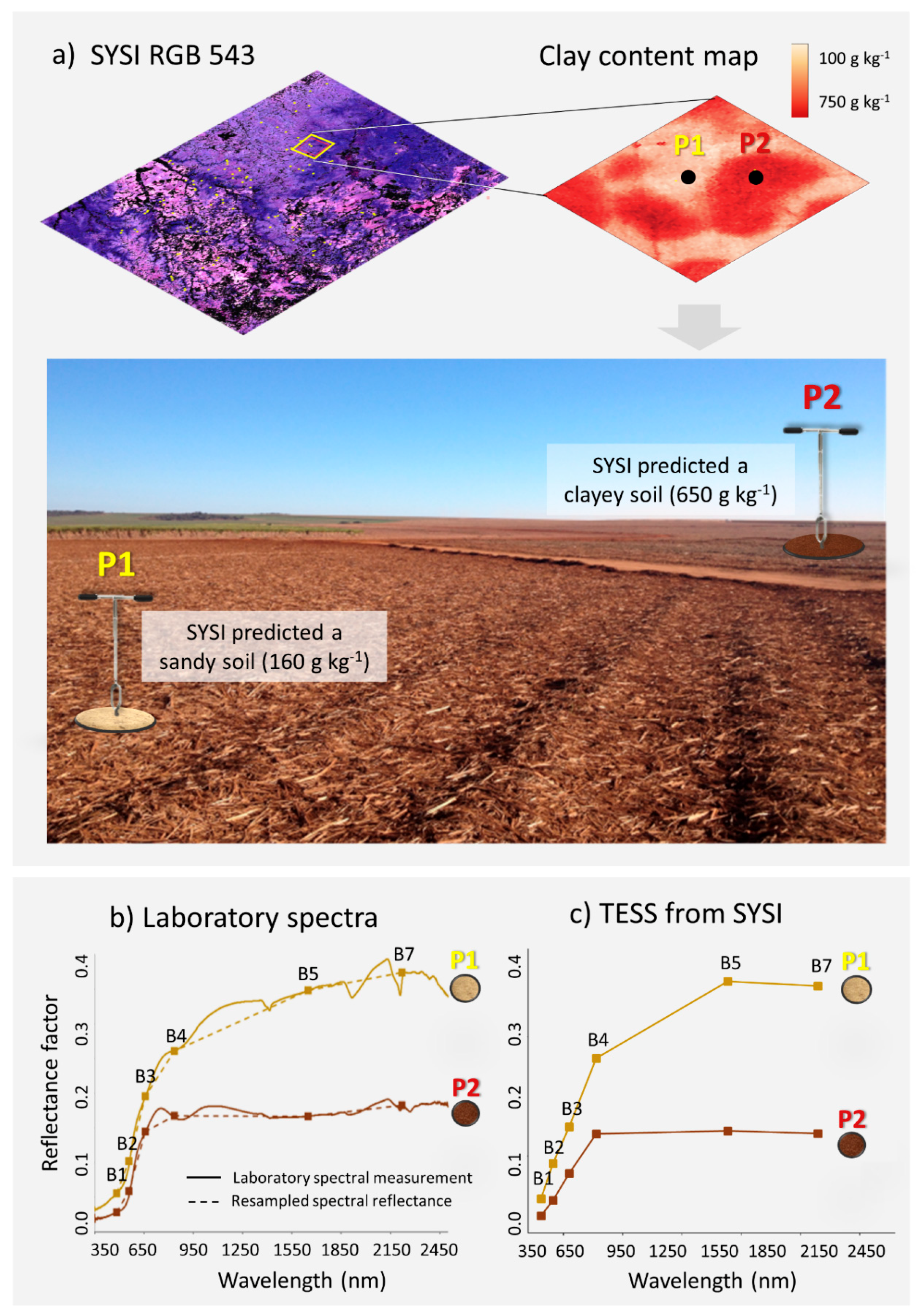
3.1. Characterization of Spectral Patterns of Soils from Ground to Space

The characterization of spectral curves from ground to satellite level (Figure 3) provides the bases for understanding prediction results. The lower intensity for clayey soils is due to energy absorption by iron oxide minerals (hematite) and other opaque minerals (i.e., magnetite and ilmenite). Soils with higher iron oxide content are derived from basalt [51]. When these minerals are absent in the soil, higher quartz content causes a strong increase in reflectance from B3 to B4, with a peak at B5. The spectral curves of clayey samples present low reflectance intensity across the spectrum, with a typical flat shape, which is different than sandy soils with an increasing reflectance shape [52].

The main, albeit slight, difference between convolved spectral measurements and TESS is observed in B1, B5, and B7 (Figure 3). The decrease of intensity from B5 to B7 being stronger in the TESS information is due to field conditions, since the information came from a pixel [53]. Nevertheless, spectral shapes from the laboratory and image are very similar, which indicates low moisture influence. The resampling of satellite data from laboratory measurements removed the absorption features present in the spectral measurements, preventing the detection of specific features for mineral identification. It can be observed that from B1 to B5, the clayey signature is almost flat, and as soil becomes sandy, it demonstrates a strong increase in B5 (due to quartz). These observations are in agreement with those of Demattê et al. [54] and Franceschini et al. [6]. Moreover, as the laboratory information is measured under controlled conditions, the similarity with TESS reinforces the robust processing of GEOS3.

Principal component (PC) analysis yielded similar transformations between laboratory spectral measurements and TESS data (Figure 4), grouping different particle size distributions along the two principal components, similar to the results of Lacerda et al. [55]. As the particle size distribution changes, samples shift slightly to the right, increasing the dispersion of the second component (Figure 4a). The same behavior occurred for TESS samples (Figure 4b). The increasing dispersion of the second component expresses the quartz influence in the infrared spectral reflectance. Meanwhile, clayey soils are related to opaque oxides from the left-hand side of the first principal component (Figure 4a,b). In the characterization of the textural classes, there was no difference between the weights for the six bands (see expression in Figure 4) in both spectral measurements resampled to multispectral satellite data. The loadings of the six factors (Bands 1, 2, 3, 4, 5, and 7) for PC1 were similar (approximately 0.40), as can be seen in the expression in Figure 4a,b. This shows that all bands are important for the differentiation of textural classes. Additionally, PC1 presents 92% and 93% of the proportion of variance for resampled and satellite data (Figure 4), respectively.

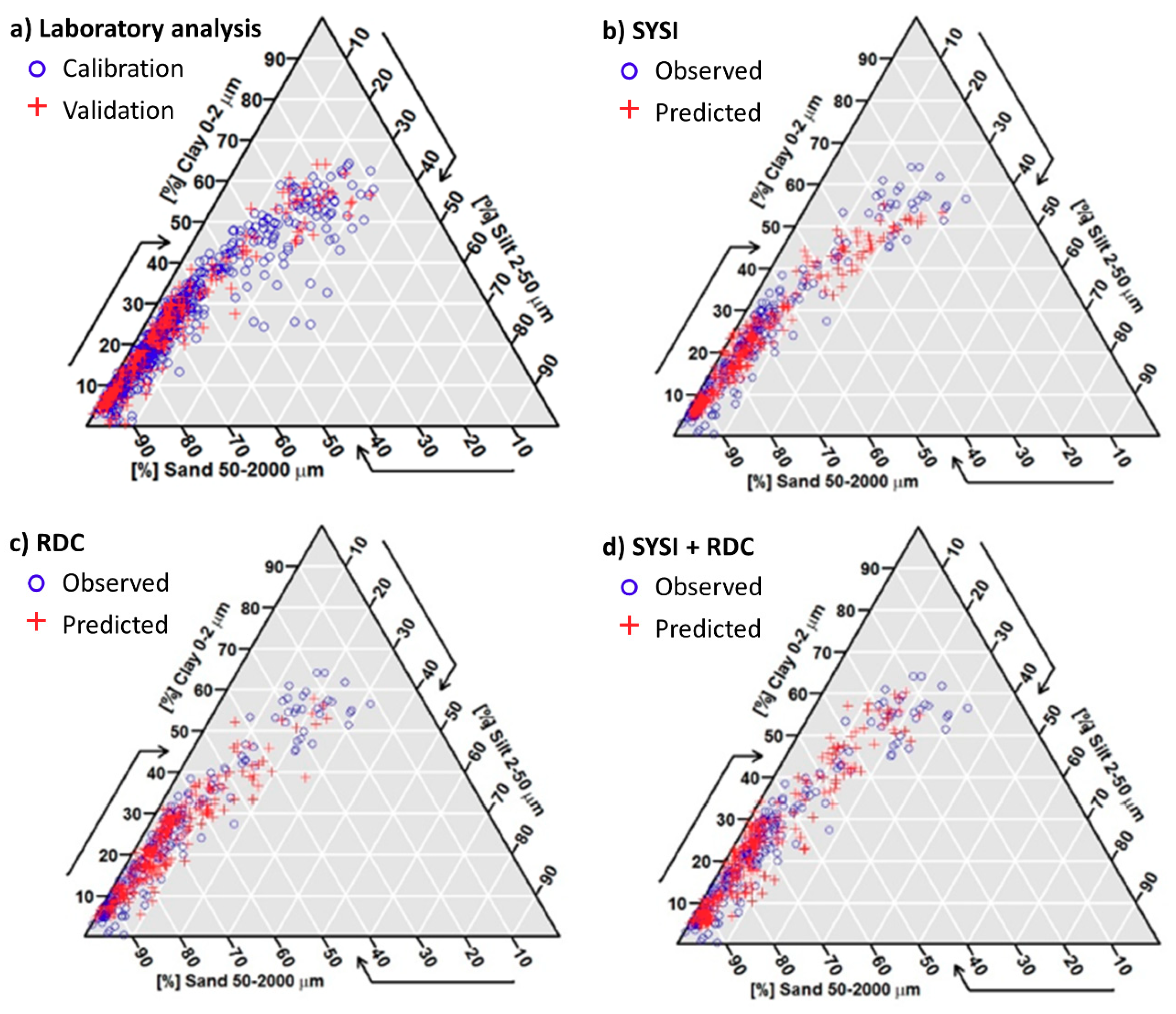
3.2. Performance of Clay and Sand Content Predictions

Comparing the models, the Cubist algorithm was more accurate than RF for clay and sand content prediction (

Table 3. Prediction validation statistics of clay and sand attributes applying Cubist and Random Forest models using a hyperspectral sensor in the laboratory, multispectral resampling in the laboratory, relief-derived covariates (RDC), Synthetic Soil Image (SYSI), and SYSI plus RDC.

Attribute	Algorithm	Parameters	R2 *	RMSE *	RPD *	RPIQ *
Clay	Random Forest	Laboratory spectral measurements	0.79	74.25	2.17	1.56
		Resampled to multispectral	0.81	70.29	2.29	1.65
		RDC	0.61	97.73	1.61	1.16
		SYSI	0.81	67.47	2.33	1.67
		SYSI + RDC	0.82	67.04	2.35	1.69
	Cubist	Laboratory spectral measurements	0.86	59.02	2.73	1.97
		Resampled to multispectral	0.83	65.79	2.45	1.76
		RDC	0.64	93.44	1.69	1.21
		SYSI	0.83	65.01	2.42	1.74
		SYSI + RDC	0.83	65.36	2.41	1.73
Sand	Random Forest	Laboratory spectral measurements	0.81	94.56	2.30	1.19
		Resampled to multispectral	0.83	89.78	2.42	1.25
		RDC	0.63	128.52	1.65	0.81
		SYSI	0.82	89.21	2.38	1.17
		SYSI + RDC	0.82	89.54	2.37	1.16
	Cubist	Laboratory spectral measurements	0.87	79.29	2.74	1.42
		Resampled to multispectral	0.85	83.33	2.61	1.35
		RDC	0.65	125.69	1.69	0.83
		SYSI	0.86	79.99	2.65	1.30
		SYSI + RDC	0.85	82.66	2.57	1.26

R²: Coefficient of Determination; * RMSE: Root-Mean-Square Error (g kg⁻¹); RPD: Ratio of Performance to Deviation; RPIQ: Ratio of Performance to Interquartile Range.

). The decrease in error (RMSE) using Cubist was approximately 20 g kg⁻¹ when using the laboratory spectral reference models, regardless of particle size fraction, while for the SYSI and the other approaches, the decrease in RMSE was between 2 and 10 g kg⁻¹ (Table 3). Although it was not our intention to compare the accuracy of Cubist with RF as both are similar machine learning approaches with superior performance [56,57], the Cubist algorithm was chosen as the best global predictor (RMSE minimization) to be used as the standard algorithm for clay and sand mapping over the study area. Predictions were better for clay than for sand content (Table 3). The sand RMSE was over 100 g kg⁻¹ in some approaches, but was reasonable for clay, although it had been expected that sand estimates would be better than clay estimates due to the higher representativeness of this fraction in the area. The best clay prediction was achieved by applying Cubist with the laboratory spectral reference data (R² = 0.86, RMSE = 59.02 g kg⁻¹, RPD = 2.73, RPIQ = 1.97), which provided a better representation of soil variability. The use of laboratory spectral reference data to estimate clay and sand content was applied to compare the performance of SYSI. Indeed, these results indicated similar performance, despite the limited resolution of the multispectral data. The use of laboratory spectral information has been previously demonstrated to be a good alternative for soil characterization and the prediction of soil properties [58].

A fair comparison between the approaches was made using the laboratory spectral resampled data (Table 3). The laboratory convolved reflectance produced similar results to SYSI and SYSI plus RDC. The best accuracies were achieved using Cubist with only the SYSI bands as predictors (Table 3, RMSE = 65.01 g kg⁻¹ clay and RMSE = 79.99 g kg⁻¹ sand). The accuracies were even close to the laboratory spectral data for estimating sand (Table 3, RMSE = 79.29 g kg⁻¹). The results from applying the combination of SYSI with RDC did not differ from those from SYSI itself (R² of 0.83 and 0.83, respectively, for clay; R² of 0.85 and 0.86, respectively, for sand). The prediction using only the RDC had the lowest R², RPD, and RPIQ (Table 3). Predicting clay using only terrain covariates resulted in R² values of 0.61 and 0.64 with the highest RMSE values of 97.73 and 93.44 g kg⁻¹ for RF and Cubist models, respectively. Moreover, the prediction of sand was slightly superior, reaching R² values of 0.63 and 0.65, and RMSE values of 128.52 and 125.69 g kg⁻¹. Henderson et al. [21] reported similar results in clay quantification using covariates derived from digital elevation models. The authors obtained an R² of 0.44 and Stępień et al. [59] found an R² of 0.2 using elevation. Landrum et al. [60] found a strong relationship between relief and clay content for soils in the northeast region of Brazil. The influence of topography on soil properties is widely discussed in Florinsky et al. [61]. In fact, the parameters of relief provide a moderate understanding of soil–landscape relationships, while the satellite images added detailed information representing the study area. Ben-Dor et al. [62] conducted an extensive literature review on the importance of satellite imagery to evaluating and characterizing soils. Nanni et al. [63] found a close relationship between satellite and field reference data, highlighting the importance of spectral reflectance for quantifying soil properties.

Several approaches have been used to map topsoil clay, such as using the vegetation index [64], airborne hyperspectral soil data of single images [65], terrain attributes, geology-based stratification [30], and electromagnetic induction techniques [66], among others. Additionally, the clay fraction has also been quantified using multispectral satellite sensors and laboratory spectral sensors (Table 1). These results can be discussed with our findings. Ahmed and Iqbal [67] found a good relationship between Bands 4 and 6 from Landsat 5 TM for clay estimation (R² = 0.509 and RMSE = 5.02%), but lower than the result found in Table 3 (R² = 0.83, RMSE = 65.01 g kg⁻¹). The prediction of clay in the laboratory usually produces better results than other sensors (satellite), in accordance with the study by Ahmed and Iqbal [67], who found an R² reaching a maximum of 0.90. Their result, however, is not far from our findings (R² = 0.86 and RMSE = 59.02 g kg⁻¹). Laboratory spectral data have a strong relationship with soil constituents due to improved experimental conditions [58,68,69], but several bands are used in the models. Despite this, the present study indicates that only a few bands would be sufficient to quantify clay and sand, which confirms the importance of this tool for mapping large areas using images [62].

At satellite sensors (i.e., at approximately 800 km distance from the targets), R² performance decreases [70]. Indeed, Coleman et al. [7] started with intermediate performances, reaching an R² of 0.4 for clay mapping using Landsat. Khalil et al. [71] reached an R² of 0.4 for the same attribute using a single image. Furthermore, the study by Shabou et al. [24] was based on 100 soil samples and a dataset of four Landsat TM scenes, reporting an R² of 0.65 and an RMSE of 100 g kg⁻¹ for clay. These accuracies were lower than those found in the present study (R² = 0.83 and RMSE = 65.01 g kg⁻¹) because here we applied 919 soil samples to 151 Landsat images. Our results can be directly related to the spectral morphology evaluation (Figure 3), which confirms that moisture from field measurements did not significantly interfere in the dataset. As stated by Ackerson et al. [72], when soil samples have differences in moisture, they do not have a linear relationship with the property to be estimated and, thus, there is no correlation. We could only depict these details because of the descriptive evaluation of the spectra, which assists in deciding whether the pixel is from soils as a clinical evaluation and not just a mathematical artifact.

In general, we have observed in previous studies that the R² values for clay prediction, using all kinds of sensors, range from approximately 0.2 to 0.9. The spectral sensors with fewer bands, like IKONOS, have lower results. It is evident that the scientific community emphasizes the use of hyperspectral data for soil mapping using, for instance, the airborne hyperspectral imaging spectrometer (HyperSpecTIR) [73] and the airborne hyperspectral sensor 160 (AHS) [74]. However, it is also evident that the use of multispectral satellite data can achieve good performance similar to that of laboratory spectral data [65,75]. These results show that despite the higher efficiency expected for hyperspectral sensors, it is not only the number of bands that matter for estimating clay and sand content, but also having bands at key wavelengths related to soil properties.

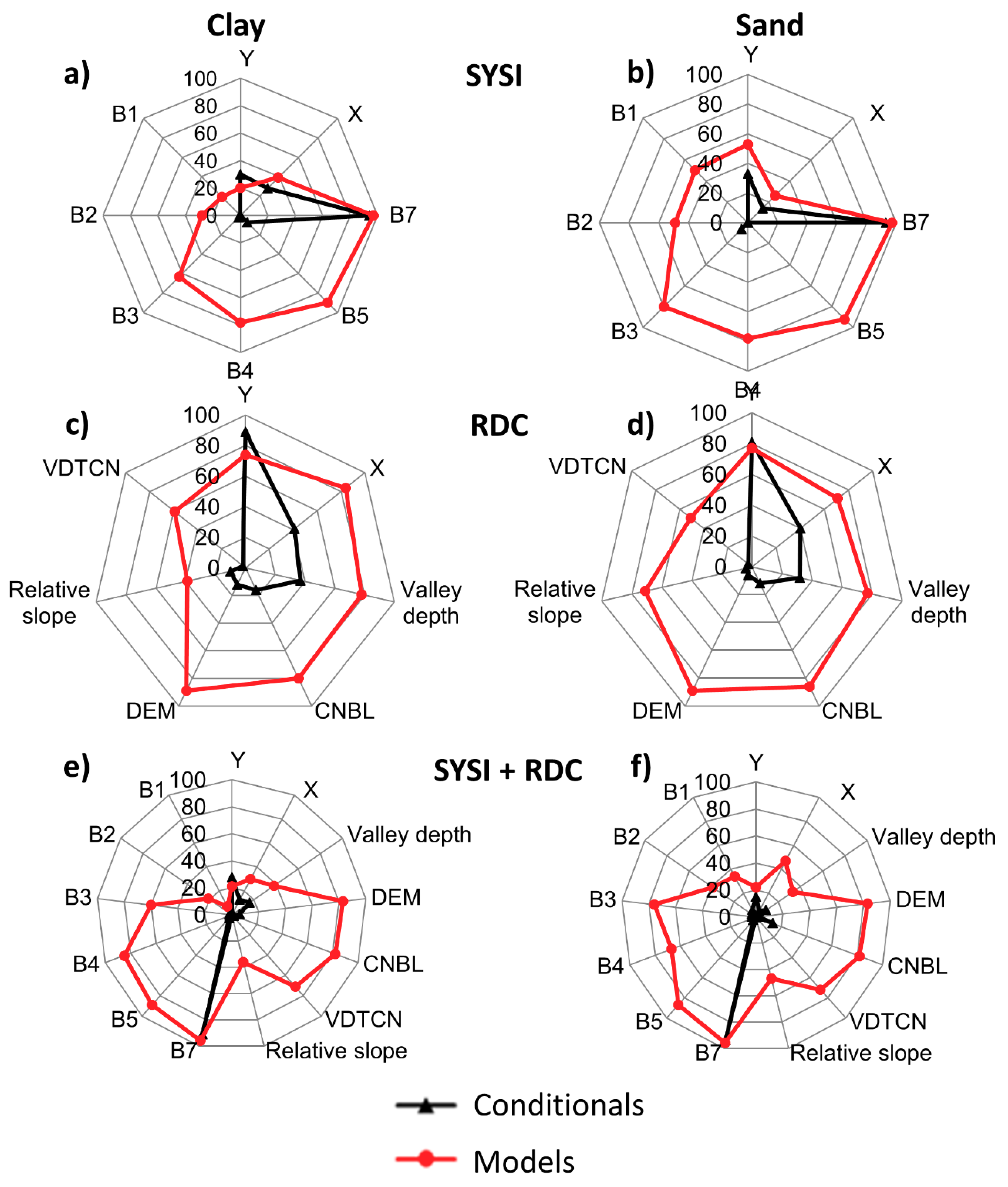
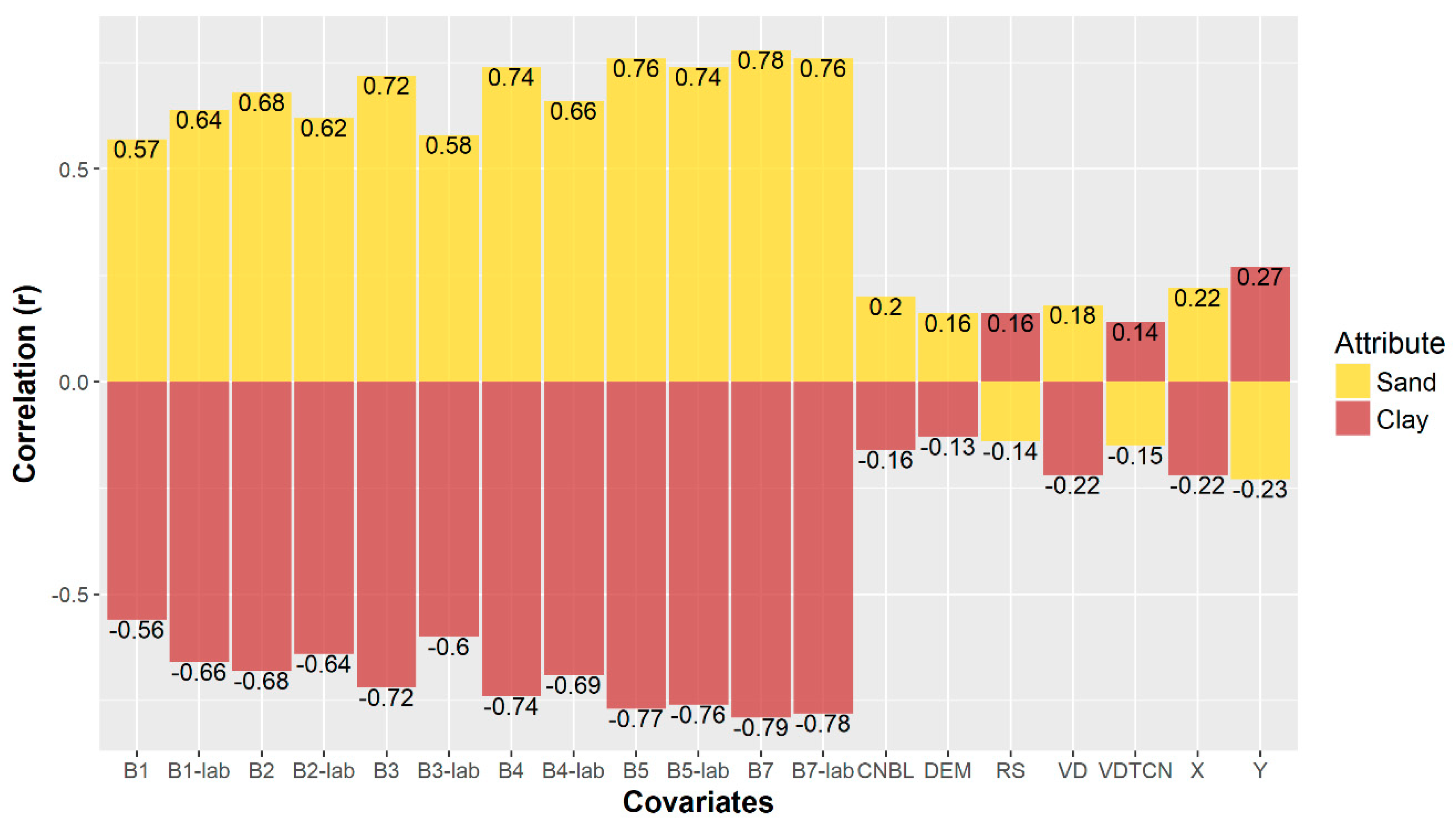
3.3. Variable Importance for Mapping Soil Attributes

Using the Cubist model and only the SYSI, B7 was found to be the most important covariate in the prediction of clay and sand (Figure 5a,b). Bands 5, 4, and 3 were also highly important to both attribute models. Bands 2 and 1 along with X and Y coordinates provided a slight contribution to the prediction of both soil attributes. Bands of the visible spectral region participated more in sand estimation as this soil particle is strongly related to the high albedo of quartz, while clay content is related to energy absorption by its minerals.

The high dependence of spatial coordinates showed contrasting results for the RDC covariates. Some parameters of RDC showed high participation in clay and sand estimation (Figure 5c,d). However, for clay quantification, the highest participation for conditional rules was from the Y (89%) and X coordinates (41%), indicating strong control from unknown factors, possibly geology. In the regression models of Cubist trees, the variable with the highest contribution was the DEM with 89% inclusion, followed by X coordinate, CNBL, valley depth, Y coordinate, and VDTCN. The contributions for sand models were similar (Figure 5d). The difference was that the relative slope had higher participation in sand models than in clay models.

For the use of the SYSI plus RDC (Figure 5e,f), B7 was the most important covariate for the Cubist conditional rules for both clay and sand models. Subsequently, for all other conditional variables, a low contribution was observed. For the regression part of Cubist, B7 was the most used covariate (>90%), followed by B5, with 89% and 87% for clay and sand modelling, respectively. These SWIR bands (B5 and B7) are still most frequently employed in both attribute estimates, indicating the strong role of this spectral region in the prediction of clay and sand attributes. Although the spectral resolution of Landsat 5 is coarse, the SWIR spectral region contains a relative contribution from the clay mineral absorption feature, which may explain why these bands were important for the attribute estimation [76].

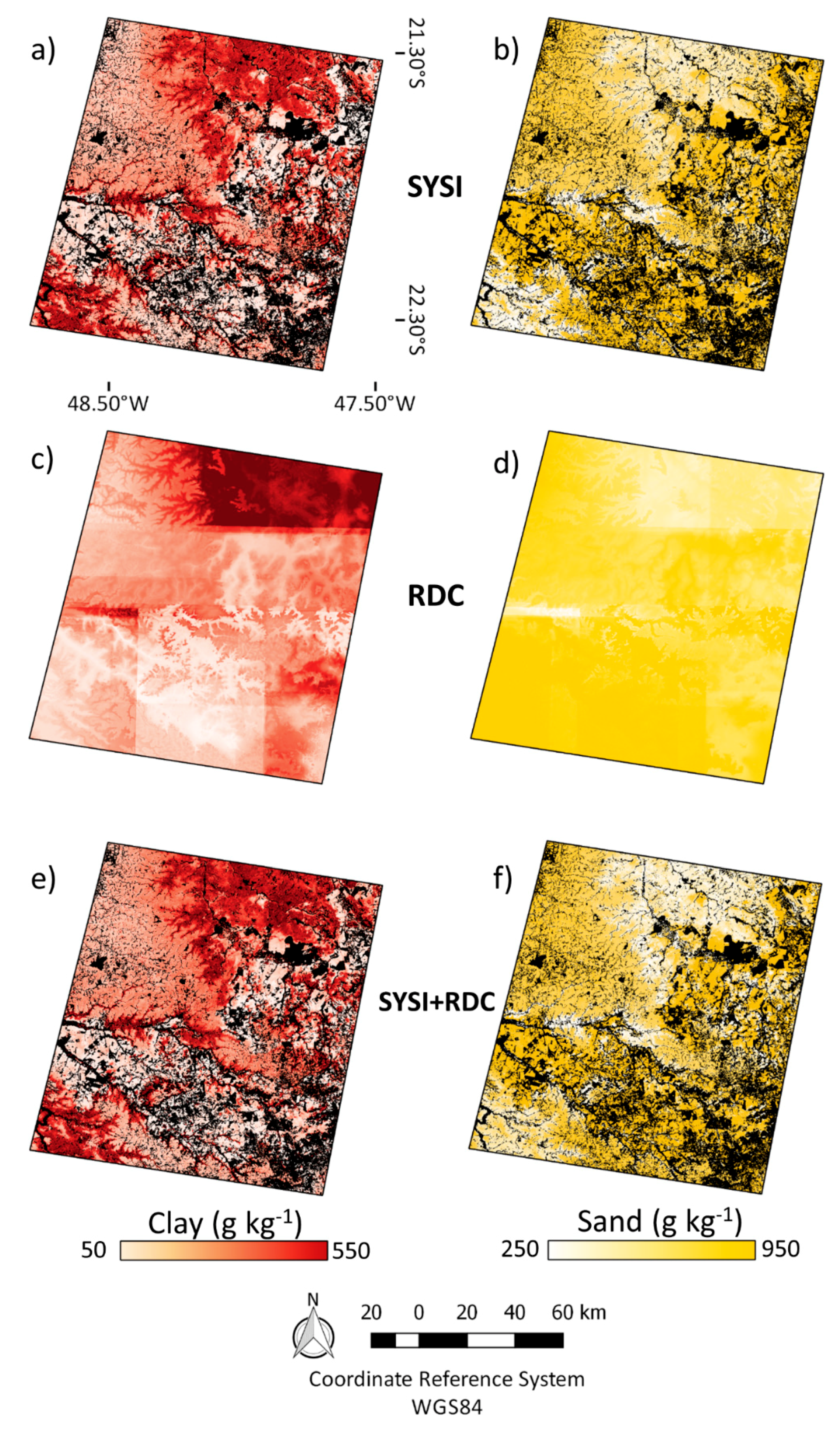
3.4. Clay and Sand Content Maps

In both datasets, most soil samples present high sand content and low silt (Figure 6a). Clay distribution is highly concentrated between 100 and 300 g kg⁻¹. Regarding all samples, 37% were classified as very sandy and sandy, 43% were loamy in texture, and 20% were classified as clayey. The variability of the particle size content is due to geological influences, as the soils of the region are formed by different parent materials, from igneous (basalt) to sedimentary rocks (sandstones and other mixes). The prediction of soil particle size distribution had different performances, although the samples were uniformly represented in the validation dataset (Figure 6a). Comparing the predictions, all the strategies had a slight tendency to underestimate the clayey samples (Figure 6b,c), except for the use of SYSI plus RDC, which improved representativeness of clayey-textured soils (Figure 6d).

The clay and sand content maps were produced using the Cubist model. This model performed better than did the RF based on the validation parameters (Table 3). It is important to note that the maps were produced using global predictors instead of spatial prediction functions, which did not consider spatial dependence for the estimations. Because the Cubist algorithm combines the use of decision rules and multiple linear regression to calibrate a model, only the maps that used SYSI had better visual continuity. Spatial continuity is the ability to represent surface variations at finer scales (Figure 7a,b,e,f). The maps with only RDC (Figure 7c,d) provided satisfactory performance, albeit with poor visual continuity due to the presence of large artifacts created by Cubist computation [77].

Terrain inference has usually been used to map soils because most of the surface is covered by vegetation and DEMs are globally available to users. However, the use of relief landforms is insufficient when it comes to explaining variations in soils along the landscape. Thus, spectral features related to mineralogical characteristics of soils may improve predictions in digital soil mapping. Reflectance factors derived from the SYSI and laboratory data show high linear relationships with clay and sand content for the full VIS-NIR-SWIR spectral bands (Figure 8). Spectral reflectance reached correlations of at least 0.45 and 0.57 with sand and clay content, respectively, with a maximum of 0.78 for clay. The RDC covariates had poor to intermediate associations. Nevertheless, the integration of RDCs with other kinds of data has been demonstrated to be a useful strategy for soil mapping [78]. It is unusual that satellite data achieve similar results to laboratory results. Considering our results, the use of the SYSI shows great potential for soil mapping, and the spatial trends from the images can increase the prediction accuracy of unmapped regions.

It is worth mentioning that the predicted maps using SYSI have consistency in the field. Figure 9a shows a study case illustrating the variation of clay within a relief landform, which could not be estimated using only the relief parameters. The laboratory (Figure 9b) and SYSI (Figure 9c) spectral patterns confirm that the two locations have different soils, with 160 and 650 g kg⁻¹ of clay estimated from the physical laboratory analysis. The illustration shows an example in which the relief would not be able to detect this variation when the region has the same relief parameters (elevation, slope, and others). In this study we provided a system to process multitemporal and multispectral satellite images to aid soil mapping. However, using satellite platforms (e.g., using Landsat) is a challenging task, as the sensor is located 800 km away from the surface with coarse spatial resolution (where spectral reflectance mixtures represent different materials within the pixel) and limited spectral resolution. Additionally, several factors can impact soil reflectance, such as atmospheric attenuation, ground surface roughness, presence of topographic shade, rocks, tree stumps, crops, and crop stubble or debris.

It is important to state that the key points of GEOS3 are based on image selection, the evaluation of the spectral signature, and validation indicators. The foremost contribution of SYSI to digital soil mapping is based on the empirical quantitative description of soil formation factors in the scorpan model [10]. As we have shown, SYSI is innovative and can play an important role in predicting topsoil attributes. Thus, SYSI can be considered as a new source of s for scorpan for predicting soil classes and/or attributes. In fact, McBratney et al. [10] pointed out that the s factor is expected to increase in importance for soil predictions as technology enhances.

4. Conclusions

The spectral signature obtained from the Synthetic Soil Image (SYSI) presented very similar patterns to the equivalent spectral signature of the laboratory data. From clayey to sandy texture, the spectral signature moved from flat low reflectance to a strong increase after Band 4, respectively. The quantification of clay and sand contents using Temporal Synthetic Spectral Reflectance (TESS) well matched the respective georeferenced location of the laboratory spectral samples. This supported the robustness of the TESS collected along the time series.

The topsoil prediction of clay and sand fractions using the SYSI presented higher-accuracy results than using Relief-Derived Covariates (RDC) alone. The attribute maps originating from the RDC approach presented spatial artifacts, despite their significance for the soil–landscape relationship. The integrated approach of the SYSI + RDC also produced accurate predictions, albeit ones that were similar to the SYSI alone. Relief is important, but it uses inferential, empirical, or mathematical approaches to estimate a soil attribute, while the SYSI is based on the availability of remote sensing spectral reflectance measurements at different times which are then used to achieve spatially continuous results rather than modeling, interpolating, or inferencing its reflectance. Furthermore, the SYSI performance was quite similar to the laboratory reference modelling results, demonstrating its strong capability for soil mapping.

TESS has provided novel information because it gives the user the capacity to evaluate the morphology of the object’s spectral signature, as information from specific points, to make an adequate decision. In addition, TESS provides a first impression of soil texture through spectral signature evaluation and SYSI supports this with the precise variation of the soil characteristics along the landscape.

The paradigm asserted by many users that soils cannot be evaluated from images because they are usually covered by vegetation is partially true. The GEOS3 method depicts images from different periods and could fill gaps that were covered with vegetation in other periods with bare soil, thus producing continuous spatial attribute maps. In forestry areas, this technique will certainly have more limitations and its usefulness will be situationally dependent.

Looking towards the future, the technique can be applied to optimizing other digital mapping projects of soils all over the world. The results are promising because they may assist in mapping large areas with bare soils occurring due to agriculture and/or anthropogenic action, degradation, and climate processes.

References

1. Mantel, S.; Schulp, C.J.E.; van den Berg, M. Modelling of Soil Degradation and Its Impact on Ecosystem Services Globally, Part 1: A Study on the Adequacy of Models to Quantify Soil Water Erosion for Use within the IMAGE Modeling Framework; Report; ISRIC―World Soil Information: Wageningen, The Netherlands, 2014. [Google Scholar]
2. Rząsa, S.; Owczarzak, W. Methods for the Granulometric Analysis of Soil for Science and Practice. Pol. J. Soil Sci. 2015, 46, 1. [Google Scholar] [CrossRef]
3. Ben-Dor, E.; Banin, A. Near-Infrared Analysis as a Rapid Method to Simultaneously Evaluate Several Soil Properties. Soil Sci. Soc. Am. J. 1995, 59, 364. [Google Scholar] [CrossRef]
4. Nawar, S.; Buddenbaum, H.; Hill, J.; Kozak, J.; Mouazen, A.M. Estimating the soil clay content and organic matter by means of different calibration methods of vis-NIR diffuse reflectance spectroscopy. Soil Tillage Res. 2016, 155, 510–522. [Google Scholar] [CrossRef]
5. Viscarra Rossel, R.A. Fine-resolution multiscale mapping of clay minerals in Australian soils measured with near infrared spectra. J. Geophys. Res. 2011, 116, F04023. [Google Scholar] [CrossRef]
6. Franceschini, M.H.D.; Demattê, J.A.M.; Sato, M.V.; Vicente, L.E.; Grego, C.R. Abordagens semiquantitativa e quantitativa na avaliação da textura do solo por espectroscopia de reflectância bidirecional no VIS-NIR-SWIR. Pesqui. Agropecuária Bras. 2013, 48, 1569–1582. [Google Scholar] [CrossRef] [Green Version]
7. Coleman, T.L.; Agbu, P.A.; Montgomery, O.L.; Gao, T.; Prasad, S. Spectral band selection for quantifying selected properties in highly weathered soils. Soil Sci. 1991, 151, 355–361. [Google Scholar] [CrossRef]
8. Mouazen, A.M.; Maleki, M.R.; De Baerdemaeker, J.; Ramon, H. On-line measurement of some selected soil properties using a VIS–NIR sensor. Soil Tillage Res. 2007, 93, 13–27. [Google Scholar] [CrossRef]
9. Morellos, A.; Pantazi, X.-E.; Moshou, D.; Alexandridis, T.; Whetton, R.; Tziotzios, G.; Wiebensohn, J.; Bill, R. Machine learning based prediction of soil total nitrogen, organic carbon and moisture content by using VIS-NIR spectroscopy. Biosyst. Eng. 2016, 152, 104–116. [Google Scholar] [CrossRef]
10. McBratney, A.B.; Mendonça Santos, M.L.; Minasny, B. On digital soil mapping. Geoderma 2003, 117, 3–52. [Google Scholar] [CrossRef]
11. Vasques, G.M.; Demattê, J.A.M.; Viscarra Rossel, R.A.; Ramírez López, L.; Terra, F.S.; Rizzo, R.; De Souza Filho, C.R. Integrating geospatial and multi-depth laboratory spectral data for mapping soil classes in a geologically complex area in southeastern Brazil. Eur. J. Soil Sci. 2015, 66, 767–779. [Google Scholar] [CrossRef]
12. Islam, K.; Singh, B.; McBratney, A. Simultaneous estimation of several soil properties by ultra-violet, visible, and near-infrared reflectance spectroscopy. Aust. J. Soil Res. 2003, 41, 1101. [Google Scholar] [CrossRef]
13. Pirie, A.; Singh, B.; Islam, K. Ultra-violet, visible, near-infrared, and mid-infrared diffuse reflectance spectroscopic techniques to predict several soil properties. Aust. J. Soil Res. 2005, 43, 713. [Google Scholar] [CrossRef]
14. Veum, K.S.; Sudduth, K.A.; Kremer, R.J.; Kitchen, N.R. Estimating a Soil Quality Index with VNIR Reflectance Spectroscopy. Soil Sci. Soc. Am. J. 2015, 79, 637. [Google Scholar] [CrossRef]
15. Wang, C.; Pan, X. Estimation of Clay and Soil Organic Carbon Using Visible and Near-Infrared Spectroscopy and Unground Samples. Soil Sci. Soc. Am. J. 2016, 80, 1393. [Google Scholar] [CrossRef]
16. O’Rourke, S.M.; Minasny, B.; Holden, N.M.; McBratney, A.B. Synergistic Use of Vis-NIR, MIR, and XRF Spectroscopy for the Determination of Soil Geochemistry. Soil Sci. Soc. Am. J. 2016, 80. [Google Scholar] [CrossRef]
17. Conforti, M.; Matteucci, G.; Buttafuoco, G. Using laboratory Vis-NIR spectroscopy for monitoring some forest soil properties. J. Soils Sediments 2017. [Google Scholar] [CrossRef]
18. Bhering, S.B.; Chagas, C.d.S.; Carvalho Junior, W.d.; Pereira, N.R.; Calderano Filho, B.; Pinheiro, H.S.K. Mapeamento digital de areia, argila e carbono orgânico por modelos Random Forest sob diferentes resoluções espaciais. Pesqui. Agropecuária Bras. 2016, 51, 1359–1370. [Google Scholar] [CrossRef] [Green Version]
19. Adeline, K.R.M.; Gomez, C.; Gorretta, N.; Roger, J.-M. Predictive ability of soil properties to spectral degradation from laboratory Vis-NIR spectroscopy data. Geoderma 2017, 288, 143–153. [Google Scholar] [CrossRef] [Green Version]
20. Dotto, A.C.; Dalmolin, R.S.D.; ten Caten, A.; Grunwald, S. A systematic study on the application of scatter-corrective and spectral-derivative preprocessing for multivariate prediction of soil organic carbon by Vis-NIR spectra. Geoderma 2018, 314. [Google Scholar] [CrossRef]
21. Henderson, B.L.; Bui, E.N.; Moran, C.J.; Simon, D.A.P. Australia-wide predictions of soil properties using decision trees. Geoderma 2005, 124, 383–398. [Google Scholar] [CrossRef]
22. Nanni, M.R.; Demattê, J.A.M. Comportamento da linha do solo obtida por espectrorradiometria laboratorial para diferentes classes de solo. Rev. Bras. Ciência do Solo 2006, 30, 1031–1038. [Google Scholar] [CrossRef] [Green Version]
23. Fiorio, P.R.; Demattê, J.A.M.; Nanni, M.R.; Formaggio, A.R. Diferenciação espectral de solos utilizando dados obtidos em laboratório e por sensor orbital. Bragantia 2010, 69, 453–466. [Google Scholar] [CrossRef] [Green Version]
24. Shabou, M.; Mougenot, B.; Chabaane, Z.; Walter, C.; Boulet, G.; Aissa, N.; Zribi, M. Soil clay content mapping using a time series of Landsat TM data in semi-arid lands. Remote Sens. 2015, 7, 6059–6078. [Google Scholar] [CrossRef]
25. Chagas, C.d.S.; de Carvalho Junior, W.; Bhering, S.B.; Calderano Filho, B. Spatial prediction of soil surface texture in a semiarid region using random forest and multiple linear regressions. Catena 2016, 139, 232–240. [Google Scholar] [CrossRef]
26. Diek, S.; Fornallaz, F.; Schaepman, M.E.; de Jong, R. Barest Pixel Composite for agricultural areas using landsat time series. Remote Sens. 2017, 9, 1245. [Google Scholar] [CrossRef]
27. Forkuor, G.; Hounkpatin, O.K.L.; Welp, G.; Thiel, M.; Zhu, A.-X.; Scholten, T.; Koch, B.; Shepherd, K. High Resolution Mapping of Soil Properties Using Remote Sensing Variables in South-Western Burkina Faso: A Comparison of Machine Learning and Multiple Linear Regression Models. PLoS ONE 2017, 12, e0170478. [Google Scholar] [CrossRef] [PubMed]
28. Zhang, T.; Li, L.; Zheng, B. Estimation of agricultural soil properties with imaging and laboratory spectroscopy. J. Appl. Remote Sens. 2013, 7, 073587. [Google Scholar] [CrossRef]
29. Castaldi, F.; Palombo, A.; Santini, F.; Pascucci, S.; Pignatti, S.; Casa, R. Evaluation of the potential of the current and forthcoming multispectral and hyperspectral imagers to estimate soil texture and organic carbon. Remote Sens. Environ. 2016, 179, 54–65. [Google Scholar] [CrossRef]
30. Samuel-Rosa, A.; Dalmolin, R.S.D.; Miguel, P. Building predictive models of soil particle-size distribution. Rev. Bras. Ciência do Solo 2013, 37, 422–430. [Google Scholar] [CrossRef] [Green Version]
31. Sumfleth, K.; Duttmann, R. Prediction of soil property distribution in paddy soil landscapes using terrain data and satellite information as indicators. Ecol. Indic. 2008, 8, 485–501. [Google Scholar] [CrossRef]
32. Odeh, I.O.; McBratney, A.B.; Chittleborough, D.J. Spatial prediction of soil properties from landform attributes derived from a digital elevation model. Geoderma 1994, 63, 197–214. [Google Scholar] [CrossRef]
33. Demattê, J.A.M.; Fongaro, C.T.; Rizzo, R.; Safanelli, J.L. Geospatial Soil Sensing System (GEOS3): A powerful data mining procedure to retrieve soil spectral reflectance from satellite images. Remote Sens. Environ. 2018, 212, 161–175. [Google Scholar] [CrossRef]
34. Alvares, C.A.; Stape, J.L.; Sentelhas, P.C.; de Moraes Gonçalves, J.L.; Sparovek, G. Köppen’s climate classification map for Brazil. Meteorol. Zeitschrift 2013, 22, 711–728. [Google Scholar] [CrossRef]
35. IUSS Working Group WRB. World Reference Base for Soil Resources 2014, update 2015. International Soil Classification System for Naming Soils and Creating Legends for Soil Maps; Working Group WRB, Ed.; World Soil Resources Reports No. 106.; FAO: Rome, Italy, 2015; ISBN 978-92-5-108369-7. [Google Scholar]
36. Donagemma, G.K.; Campos, D.V.B. de; Calderano, S.B.; Teixeira, W.G.; Viana, J.H.M. Manual de Métodos de Análise de Solo, 2nd ed.; Embrapa Solos: Rio de Janeiro, Brazil, 2011. [Google Scholar]
37. Lehnert, L.W.; Meyer, H.; Bendix, J. Hsdar: Manage, Analyse and Simulate Hyperspectral Data in R. R Packag. Version 0.4 2016. Available online: https://cran.r-project.org/web/packages/hsdar/index.html (accessed on 9 May 2016).
38. Masek, J.G.; Vermote, E.F.; Saleous, N.E.; Wolfe, R.; Hall, F.G.; Huemmrich, K.F.; Gao, F.; Kutler, J.; Lim, T.-K. A Landsat Surface Reflectance Dataset for North America, 1990–2000. IEEE Geosci. Remote Sens. Lett. 2006, 3, 68–72. [Google Scholar] [CrossRef]
39. Vermote, E.F.; El Saleous, N.; Justice, C.O.; Kaufman, Y.J.; Privette, J.L.; Remer, L.; Roger, J.C.; Tanré, D. Atmospheric correction of visible to middle-infrared EOS-MODIS data over land surfaces: Background, operational algorithm and validation. J. Geophys. Res. Atmos. 1997, 102, 17131–17141. [Google Scholar] [CrossRef] [Green Version]
40. Demattê, J.A.M.; Bellinaso, H.; Romero, D.J.; Fongaro, C.T. Morphological Interpretation of Reflectance Spectrum (MIRS) using libraries looking towards soil classification. Sci. Agric. 2014, 71, 509–520. [Google Scholar] [CrossRef] [Green Version]
41. Ben-Dor, E.; Banin, A. Evaluation of several soil properties using convolved TM spectra. In Monitoring in the Environment with Remote Sensing and GIS; Escadafal, R., Mulders, M., Thiombiano, L., Eds.; ORSTOM éditions: Paris, France, 1996; pp. 135–149. ISBN 2709913313. [Google Scholar]
42. Moura-Bueno, J.M.J.M.; Dalmolin, R.S.D.R.S.D.; ten Caten, A.; Ruiz, L.F.C.L.F.C.; Ramos, P.V.P.V.; Dotto, A.C.A.C. Assessment of Digital Elevation Model for Digital Soil Mapping in a Watershed with Gently Undulating Topography. Rev. Bras. Ciência do Solo 2016, 40. [Google Scholar] [CrossRef] [Green Version]
43. Santos, H.G.; Jacomine, P.K.T.; Anjos, L.H.C.; Oliveira, V.A.; Lumbreras, J.F.; Coelho, M.R.; Almeida, J.A.; Cunha, T.J.F.; Oliveira, J.B. Sistema Brasileiro de Classificação de Solos; 3 rev. amp.; Embrapa: Brasília, Brazil, 2013; ISBN 978-85-7035-198-2. [Google Scholar]
44. Conrad, O.; Bechtel, B.; Bock, M.; Dietrich, H.; Fischer, E.; Gerlitz, L.; Wehberg, J.; Wichmann, V.; Böhner, J. System for Automated Geoscientific Analyses (SAGA) v. 2.1.4. Geosci. Model Dev. 2015, 8, 1991–2007. [Google Scholar] [CrossRef]
45. Kuhn, M.; Weston, S.; Keefer, C.; Coulter, N.; Quinlan, C. Code for C. by R. Cubist: Rule- and Instance-Based Regression Modeling. R Package Version 0.0.19. 2016. Available online: https://CRAN.R-project.org/package=Cubist (accessed on 8 May 2016).
46. Liaw, A.; Wiener, M. Classification and Regression by randomForest. R News 2002, 2, 18–22. [Google Scholar]
47. R Core Team R: A language and environment for statistical computing 2018.
48. Hijmans, R.J. Raster: Geographic Data Analysis and Modeling. R package version 2.5-8. Available online: https://CRAN.R-project.org/package=raster (accessed on 22 August 2016).
49. Bellon-Maurel, V.; Fernandez-Ahumada, E.; Palagos, B.; Roger, J.-M.; McBratney, A. Critical review of chemometric indicators commonly used for assessing the quality of the prediction of soil attributes by {NIR} spectroscopy. TrAC Trends Anal. Chem. 2010, 29, 1073–1081. [Google Scholar] [CrossRef]
50. Moeys, J. Soiltexture: Functions for Soil Texture Plot, Classification and Transformation. R package version 1.4.1. 2016. Available online: https://CRAN.R-project.org/package=soiltexture (accessed on 5 October 2016).
51. Demattê, J.A.M.; Campos, R.C.; Alves, M.C.; Fiorio, P.R.; Nanni, M.R. Visible–NIR reflectance: A new approach on soil evaluation. Geoderma 2004, 121, 95–112. [Google Scholar] [CrossRef]
52. Demattê, J.A.M.M.; Terra, F.S.d.S.; da Silva Terra, F.; Terra, F.S.d.S.; da Silva Terra, F. Spectral pedology: A new perspective on evaluation of soils along pedogenetic alterations. Geoderma 2014, 217–218, 190–200. [Google Scholar] [CrossRef]
53. Musick, H.B.; Pelletier, R.E. Response of Some Thematic Mapper Band Ratios to Variation in Soil Water Content. Photogram. Eng. Remote Sens. 1986, 1166–1661. [Google Scholar]
54. Demattê, J.A.M.; Fiorio, P.R.; Ben-Dor, E. Estimation of soil properties by orbital and laboratory reflectance means and its relation with soil classification. Open Remote Sens. J. 2009, 2, 12–23. [Google Scholar] [CrossRef]
55. Lacerda, M.; Demattê, J.; Sato, M.; Fongaro, C.; Gallo, B.; Souza, A. Tropical Texture Determination by Proximal Sensing Using a Regional Spectral Library and Its Relationship with Soil Classification. Remote Sens. 2016, 8, 701. [Google Scholar] [CrossRef]
56. Bonfatti, B.R.; Hartemink, A.E.; Giasson, E.; Tornquist, C.G.; Adhikari, K. Digital mapping of soil carbon in a viticultural region of Southern Brazil. Geoderma 2016, 261, 204–221. [Google Scholar] [CrossRef]
57. Noi, P.; Degener, J.; Kappas, M. Comparison of Multiple Linear Regression, Cubist Regression, and Random Forest Algorithms to Estimate Daily Air Surface Temperature from Dynamic Combinations of MODIS LST Data. Remote Sens. 2017, 9, 398. [Google Scholar] [CrossRef]
58. Viscarra Rossel, R.A.; Behrens, T.; Ben-Dor, E.; Brown, D.J.; Demattê, J.A.M.; Shepherd, K.D.; Shi, Z.; Stenberg, B.; Stevens, A.; Adamchuk, V.; et al. A global spectral library to characterize the world’s soil. Earth-Sci. Rev. 2016, 155, 198–230. [Google Scholar] [CrossRef] [Green Version]
59. Stępień, M.; Samborski, S.; Gozdowski, D.; Dobers, E.S.; Chormański, J.; Szatyłowicz, J. Assessment of soil texture class on agricultural fields using ECa, Amber NDVI, and topographic properties. J. Plant Nutr. Soil Sci. 2015, 178, 523–536. [Google Scholar] [CrossRef]
60. Landrum, C.; Castrignanò, A.; Mueller, T.; Zourarakis, D.; Zhu, J.; De Benedetto, D. An approach for delineating homogeneous within-field zones using proximal sensing and multivariate geostatistics. Agric. Water Manag. 2015, 147, 144–153. [Google Scholar] [CrossRef]
61. Florinsky, I.V.; Eilers, R.G.; Manning, G.R.; Fuller, L.G. Prediction of soil properties by digital terrain modelling. Environ. Model. Softw. 2002, 17, 295–311. [Google Scholar] [CrossRef]
62. Ben-Dor, E.; Chabrillat, S.; Demattê, J.A.M.; Taylor, G.R.; Hill, J.; Whiting, M.L.; Sommer, S. Using Imaging Spectroscopy to study soil properties. Remote Sens. Environ. 2009, 113, S38–S55. [Google Scholar] [CrossRef]
63. Nanni, M.R.; Dematte, J.A.M.; Junior, C.A.d.S.; Romagnoli, F.; Silva, A.A.d.; Cezar, E.; Gasparotto, A.d.C. Soil Mapping by Laboratory and Orbital Spectral Sensing Compared with a Traditional Method in a Detailed Level. J. Agron. 2014, 13, 100–109. [Google Scholar] [CrossRef]
64. Demattê, J.A.M.; Sayão, V.M.; Rizzo, R.; Fongaro, C.T. Soil class and attribute dynamics and their relationship with natural vegetation based on satellite remote sensing. Geoderma 2017, 302, 39–51. [Google Scholar] [CrossRef]
65. Nouri, M.; Gomez, C.; Gorretta, N.; Roger, J.M. Clay content mapping from airborne hyperspectral Vis-NIR data by transferring a laboratory regression model. Geoderma 2017, 298. [Google Scholar] [CrossRef]
66. Triantafilis, J.; Lesch, S.M. Mapping clay content variation using electromagnetic induction techniques. Comput. Electron. Agric. 2005, 46, 203–237. [Google Scholar] [CrossRef] [Green Version]
67. Ahmed, Z.; Iqbal, J. Evaluation of Landsat TM5 Multispectral Data for Automated Mapping of Surface Soil Texture and Organic Matter in GIS. Eur. J. Remote Sens. 2014, 47, 557–573. [Google Scholar] [CrossRef] [Green Version]
68. Viscarra Rossel, R.A.; Chen, C. Digitally mapping the information content of visible-near infrared spectra of surficial Australian soils. Remote Sens. Environ. 2011, 115, 1443–1455. [Google Scholar] [CrossRef]
69. Soriano-Disla, J.M.; Janik, L.J.; Viscarra Rossel, R.A; MacDonald, L.M.; McLaughlin, M.J. The Performance of Visible, Near-, and Mid-Infrared Reflectance Spectroscopy for Prediction of Soil Physical, Chemical, and Biological Properties. Appl. Spectrosc. Rev. 2014, 49, 139–186. [Google Scholar] [CrossRef]
70. Demattê, J.; Ramirez-Lopez, L.; Rizzo, R.; Nanni, M.; Fiorio, P.; Fongaro, C.; Medeiros Neto, L.; Safanelli, J.; da S. Barros, P. Remote Sensing from Ground to Space Platforms Associated with Terrain Attributes as a Hybrid Strategy on the Development of a Pedological Map. Remote Sens. 2016, 8, 826. [Google Scholar] [CrossRef]
71. Khalil, R.Z.; Khalid, W.; Akram, M. Estimating of soil texture using landsat imagery: A case study of Thatta Tehsil, Sindh. In Proceedings of the IEEE International Geoscience and Remote Sensing Symposium (IGARSS), Beijing, China, 10–15 July 2016; pp. 3110–3113. [Google Scholar]
72. Ackerson, J.P.; Dematte, J.A.M.; Morgan, C.L.S.; Demattê, J.A.M.; Morgan, C.L.S. Predicting clay content on field-moist intact tropical soils using a dried, ground VisNIR library with external parameter orthogonalization. Geoderma 2015, 259–260, 196–204. [Google Scholar] [CrossRef]
73. Hively, W.D.; McCarty, G.W.; Reeves, J.B.; Lang, M.W.; Oesterling, R.A.; Delwiche, S.R. Use of Airborne Hyperspectral Imagery to Map Soil Properties in Tilled Agricultural Fields. Appl. Environ. Soil Sci. 2011, 2011, 1–13. [Google Scholar] [CrossRef]
74. Stevens, A.; Udelhoven, T.; Denis, A.; Tychon, B.; Lioy, R.; Hoffmann, L.; van Wesemael, B. Measuring soil organic carbon in croplands at regional scale using airborne imaging spectroscopy. Geoderma 2010, 158, 32–45. [Google Scholar] [CrossRef] [Green Version]
75. Gomez, C.; Lagacherie, P.; Coulouma, G. Regional predictions of eight common soil properties and their spatial structures from hyperspectral Vis–NIR data. Geoderma 2012, 189–190, 176–185. [Google Scholar] [CrossRef]
76. Gomez, C.; Adeline, K.; Bacha, S.; Driessen, B.; Gorretta, N.; Lagacherie, P.; Roger, J.M.; Briottet, X. Sensitivity of clay content prediction to spectral configuration of VNIR/SWIR imaging data, from multispectral to hyperspectral scenarios. Remote Sens. Environ. 2018, 204, 18–30. [Google Scholar] [CrossRef]
77. Padarian, J.; Minasny, B.; McBratney, A.B.; Dalgliesh, N. Predicting and mapping the soil available water capacity of Australian wheatbelt. Geoderma Reg. 2014, 2–3, 110–118. [Google Scholar] [CrossRef]
78. Vasques, G.M.; Coelho, M.R.; Dart, R.O.; Oliveira, R.P.; Teixeira, W.G. Mapping soil carbon, particle-size fractions, and water retention in tropical dry forest in Brazil. Pesqui. Agropecuária Bras. 2016, 51, 1371–1385. [Google Scholar] [CrossRef] [Green Version]
Figure 1. Flowchart showing the study area within the São Paulo State, Brazil, and the methodology applied.
Remotesensing 10 01555 g001
Figure 2. The Synthetic Soil Image (SYSI) (a) and Digital Elevation Model (DEM) (b) of the study area.
Remotesensing 10 01555 g002
Figure 3. Average spectral reflectance of soil texture classes expressed either by the convolved laboratory bands (obtained from the laboratory spectral measurements) or the respective Temporal Synthetic Spectral Reflectance (TESS), acquired from the Synthetic Soil Image (SYSI, satellite). Bands: B1 (450–520 nm), B2 (520–600 nm), B3 (630–690 nm), B4 (760–900 nm), B5 (1550–1750 nm), and B7 (2080–2350 nm).
Remotesensing 10 01555 g003
Figure 4. Principal component (PC) analysis of the spectral reflectance of convolved laboratory spectra (a) and Temporal Synthetic Spectral Reflectance (TESS) from the Synthetic Soil Image (SYSI) (b). The colors of samples are related to the soil texture classes.
Remotesensing 10 01555 g004
Figure 5. Variable contributions for clay and sand Cubist models using three approaches: only the Synthetic Soil Image (SYSI) (a,b), only the Relief-Derived Covariates (RDC) (c,d), and SYSI plus RDC (e,f). DEM: Elevation from Digital Elevation Model; CNBL: Distance from Channel Network to Base Level; VDTCN: Vertical Distance To Channel Network; X: Easting geographical Cartesian coordinate related to WGS84 UTM zone 23S; Y: Northing geographical Cartesian coordinate related to WGS 84 UTM zone 23S. Spectral reflectance from the Synthetic Soil Image (SYSI), equivalent to Landsat 5 Thematic Mapper spectral bands ranges (B1 to B7).
Remotesensing 10 01555 g005
Figure 6. Soil texture triangle of calibration and validation datasets (a), comparing the observed and predicted clay and sand contents from the three mapping approaches: only the Synthetic Soil Image (SYSI) (b), only the Relief-Derived Covariates (RDC) (c), and SYSI plus RDC (d). The silt percent was estimated by the difference of 100% − (sand% + clay%).
Remotesensing 10 01555 g006
Figure 7. Clay and sand content maps produced from three approaches: using only the Synthetic Soil Image (SYSI) (a,b), only the Relief-Derived Covariates (RDC) (c,d), and SYSI plus RDC (e,f). The maps refer to the models built using the Cubist algorithm. Black color represents unmapped areas.
Remotesensing 10 01555 g007
Figure 8. Pearson’s correlation between covariates and clay and sand contents. RDC: relief-derived covariates; DEM: digital elevation model; CNBL: distance from channel network to base level; RS: relative slope; VD: valley depth; VDTCN: vertical distance to channel network; X: Easting coordinate; Y: Northing coordinate. B1 to B7: spectral reflectance from the Synthetic Soil Image (SYSI) bands with the Landsat 5 TM spectral ranges. The suffix “lab” indicates the laboratory spectra convolved to Landsat 5 TM spectral bands.
Remotesensing 10 01555 g008
Figure 9. General illustration of the predicted clay map by Synthetic Soil Image (SYSI) for the same landform (a); resampled and laboratory spectral curves (b), and the Temporal Synthetic Spectral Reflectance (TESS) from the SYSI (c); B1 (450–520 nm), B2 (520–600 nm), B3 (630–690 nm), B4 (760–900 nm), B5 (1550–1750 nm), and B7 (2080–2350 nm).
Remotesensing 10 01555 g009