A Modified Change Vector Approach for Quantifying Land Cover Change


1
Institute of Space and Earth Information Science, The Chinese University of Hong Kong, Hong Kong, China
2
Institute of Space and Earth Information Science, Department of Geography and Resource Management and Shenzhen Research Institute, The Chinese University of Hong Kong, Hong Kong, China
3
State Key Laboratory of Urban and Regional Ecology, Research Center for Eco-Environmental Sciences, Chinese Academy of Sciences, Beijing 100085, China
4
University of Chinese Academy of Sciences, Beijing 100049, China
5
School of Geography, University of Leeds, Leeds LS2 9JT, UK
*
Author to whom correspondence should be addressed.
Remote Sens. 2018, 10(10), 1578; https://0-doi-org.brum.beds.ac.uk/10.3390/rs10101578
Submission received: 30 July 2018
/
Revised: 21 September 2018
/
Accepted: 26 September 2018
/
Published: 1 October 2018
Abstract
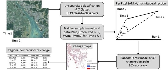
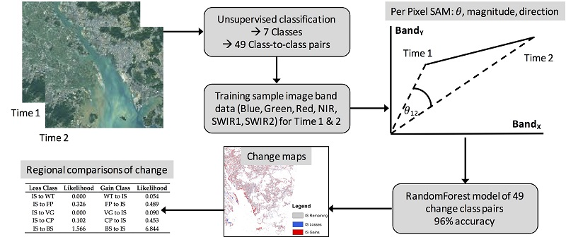
:This paper develops and applies a novel method for inferring land cover/land use (LCLU) change that combines direct multi-date classification with measures from a change vector analysis. The model predicts change directly rather than the land cover at either time, although these could be inferred. Unsupervised classifications of bi-temporal imagery were manually labeled and used to generate reference data for class-to-class changes. These were used to train a Random Forest model with inputs from the bi-temporal image bands and change vector measures (change vector direction, angle and the spectral angle) and used to generate a predicted surface of land cover change for a case study in the Pearl River Delta, China. The overall accuracy of LCLU change prediction was 96% and specific class-to-class changes had errors rates of 0–12.8%. Some errors were related the semi-automated labeling of the training data. The spectral angle variables and Near Infra-Red image bands for both years were found to be strong predictors of change. Odd ratios were used to quantify regional differences in land cover change rates in urban and peri-urban areas. The regional differences and origins of the observed errors are discussed, along with some areas of further work. The key contributions of this paper are the focus on change rather than LCLU through the construction of a model to predict changes directly and the development of an approach that provides quick, effective and informative analysis of LCLU change in support of policy and planning in rapidly urbanizing areas.
1. Introduction
Understanding land cover and land use (LCLU) change is important [1,2]. LCLU changes are caused by human activity and natural processes [2,3]. Accurate and timely measures of LCLU change can inform local decision making and planning [4]. Remote sensing data provide an opportunity to monitor land surfaces both spatially and temporally. This paper proposes and applies a change vector analysis (CVA) of land cover and land use change. It combines direct multi-date classification [5] with CVA measures (magnitude, spectral direction and spectral angle) and with image band reflectance values. These are used to train a Random Forest model of LCLU change. The predictive models of class-to-class changes are applied to bi-temporal Landsat data to estimate LCLU changes for a case study in the Pearl River Delta, China. This paper reflects a shift in emphasis in current approaches to LCLU monitoring away from a focus of LCLU states towards one of LCLU change processes, although inevitably the former are associated with the latter. It seeks to quantify change processes and, in so doing, build on approaches and philosophies being applied in large scale land cover inventories [6,7]. These focus explicitly on process (LCLU change) rather than state (the LCLU class label), and do not seek to map land cover per se, rather they consider the strength of the signal of difference in imagery over time. The analysis presented in this paper has a similar focus on the identification of LCLU change as the primary analysis objective as in [6,7] but does this using methods that can be used in resource and infrastructure poor situations. The approach is to generate and manually label bi-temporal unsupervised LCLU layers from which reference data are sampled. These are used to calculate class-to-class change vectors and image characteristics which are used as inputs to train a classification model. The model is then used to predict and label land cover change directly and to quantify rates of urbanization.
There are many different approaches to land cover change detection methods and thorough reviews of these are provided by Hussain et al. [8], Tewkesbury et al. [9] and Zhu [10]. Commonly applied approaches include image differencing (e.g., [11]), image ratio and transformation (e.g., [12]), change vector analysis (CVA) (e.g., [13,14]) and post classification comparison (PCC) (e.g., [15,16]). The PCC approach is the most widely applied and reported in the literature [9] but requires input data (classified maps) with accuracies that are beyond operational capacity of most land cover monitoring initiatives [4,17,18,19,20]. Generally, PCC should not be used, even though it is conceptually elegant. CVA approaches characterize class-to-class change vectors in bi-temporal image feature space. They require the characteristics of change to be known [8,21] and the trajectories of changes in multi-dimensional image feature space to be sufficiently distinct and statistically separable. Thus, there are three core challenges for any direct multi-date approaches to LCLU change, whether supervised or unsupervised: the need for large amounts of reference data to sufficiently characterize each bi-temporal change class, the potential for high variability of any given change and the sensitivity of any approach to image mis-registration including Landsat [22].
Because of these challenges, many large scale operational LCLU inventories have adopted approaches that first focus on identifying any LCLU change and then update baseline inventories retrospectively. Gómez et al. [23] provided a theoretical review. This generic approach represents a significant shift in the way that LCLU inventory and update are undertaken from satellite imagery (e.g., [24]), aerial photography (e.g., [25]) and historical LCLU data updates (e.g., [26]). Philosophically, these approaches represent a shift from a focus on the crisp, Boolean, object-based concept of land cover [27], to one based on processes and fields, in which the attributes or qualities of LCLU are evaluated (e.g., [21]). The focus on identifying change processes can be seen in many recent reports of large inventories [6,7] which seek to determine whether the signals of change are sufficiently strong to be accepted and if so only then are LCLU class labels retrospectively updated. They are underpinned by access to long, wide and deep archives of time series data [28] that form large spatiotemporal data cubes [29,30], and by the provision of Analysis Ready Data (ARD). ARD reduce pre-processing prior to analysis and include the latest image calibration and corrections to improve consistency and comparability of results. ARD are “stackable” such that a given pixel through time represents the same physical ground location.
However, the large-scale inventory approaches to LCLU change described above require resources and infrastructures that may be beyond many applications, especially in less developed countries, where measures of LCLU change are required to, for example, understand the dynamics of urbanization processes. PCC approaches require classified LCLU accuracies that are simply not possible, ARD are not available and the problems of variability in change signals and image co-registration persist. In this context, pragmatic, reproducible and easily applied approaches for generating reliable snapshots of LCLU change are needed. There are advantages to methods for determining LCLU change that focus only on processes rather than seeking to determine states. A modified Change Vector Analysis (CVA) offers a method that is potentially able to do this.
Classic CVA [31] determines the change in position in image feature spaces (for example, composed Landsat image bands) of LCLU objects, usually pixels, over time. At each time, the object vector from the origin is determined in the feature space. The change vector is the difference between vectors at different times, with the change vector direction indicative of the type of LCLU change and its length indicative of the magnitude of change, which together can be used to label change [32]. Magnitude is usually a simple Euclidean distance measure and is used to quantify change extent (e.g., [33,34]). The underpinning idea is that vector magnitude indicates changes in image radiance, but contains only limited thematic information, and the direction indicates the type of change. The key considerations in CVA are how to define the feature space within which the vectors are calculated—that is which image bands and variables to include—and whether to transform them. Carvalho Júnior et al. [13] noted that a 2D feature space is often defined because of the difficulty in interpreting the vectors calculated over an n-dimensional feature space [35]. However, feature space selection may be driven by the application. Bovolo and Bruzzone [32], for example, used a 2D feature space of Landsat bands 3 and 4 to map burnt area changes. Thus, determining which bands to use requires a degree of prior knowledge of the changes under investigation [35]. Because of the difficulty of working with change vectors defined in multi-dimensional feature spaces, data transformations are frequently applied to reduce the dimensionality of the data. Commonly applied transformation approaches include tasseled cap [36,37,38,39] and principle components analysis [3,40]. In both cases, the original image data are transformed to new sets of variables and care has to be given to both input selection and interpreting the meaning of the outputs [35]. A final consideration in CVA research is the use of the Spectral Angle Mapper (SAM) [13]. SAM approaches generate similarity measures for vectors defined over n-dimensional space from their inner product, and, although they do not provide information about land cover change, they have been used to inform CVA applications [13]. Bovolo et al. [35] argued that such developments in CVA have the potential for a universal change detection framework.
The aim of this research was to quantify the LCLU change processes, and not necessarily the start and end states. Two main approaches to LCLU change have been adopted: supervised and unsupervised methods [5,41]. Supervised approaches are based on supervised classification methods and require the availability of multi-temporal reference data. Unsupervised ones make a direct comparison of the two multispectral images without relying on any additional information. Here, a hybrid approach was applied which manually labeled broad scale unsupervised classifications of images at both dates. These reference data were randomly selected from the center of homogenously classified regions to avoid edge and bi-temporal image mis-registration effects which are well known in Landsat data [22]. The reference data were used to construct a set of change vectors from which vector characteristics were calculated (magnitude, spectral direction and spectral angle) for each labeled change. These were used to train statistical classifier and used to predict class-to-class change, including no change. Regional variations in LCLU change were determined using the methods described in Comber et al. [42]. This is a novel approach for determining LCLU change, one that uses measures derived from change vectors and applied to bi-temporal image data. The analysis has an explicit focus on the change vector measures, and not the individual vectors at Time 1 and Time 2.
2. Materials and Methods
2.1. Data and Study Area
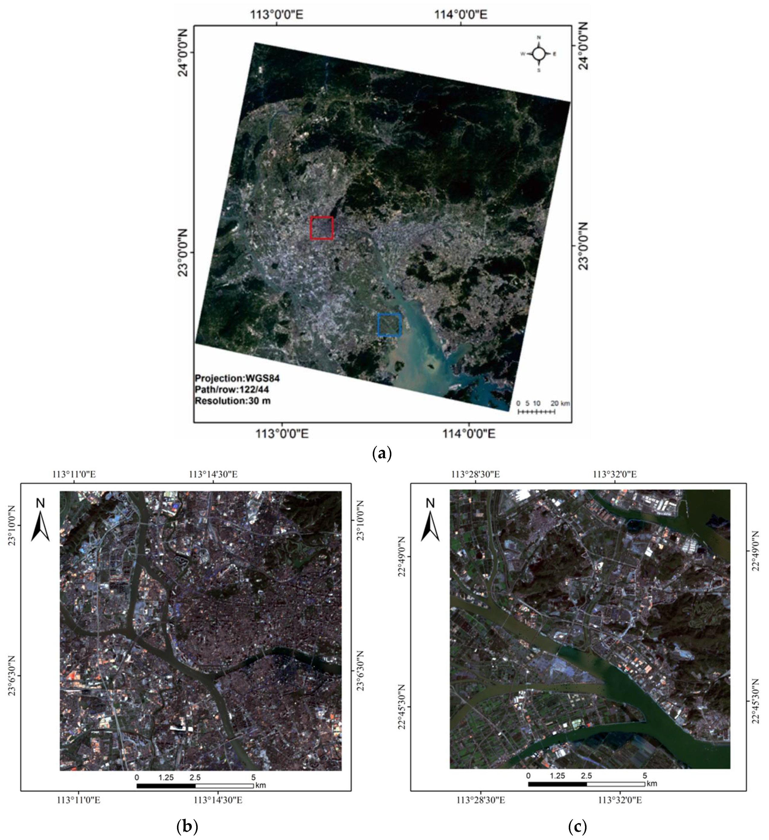
The Pearl River Delta is located in southern part of China (Figure 1a). It has a humid climate that results in rainy weather all year around and annual precipitation and average temperature of ~1500 mm and 23 °C, respectively. This region is rich in natural vegetation with a dense river and drainage network and the climate supports a variety of agricultural systems including banana, pineapple, carambola, mango and grapefruit plantations. The urban area is surrounded by natural and semi-natural land cover types. The region has a number of large, active economic centers including the cities of Guangzhou, Shenzhen and Hong Kong which have experienced long and sustained urbanization. Two sub-regions of 400 by 400 pixels with an area of 144 km2 each were selected for comparison to represent urban and peri-urban contexts (Figure 1b,c). Region 1 was characterized by high density settlements located in the core urban area and Region 2 by high levels of agricultural activities located in the peri-urban area. Both regions are subject to highly intensive human activity and disturbance and provide proto-typical examples of contrasting but common land use mixes. These two areas were selected to support a deeper discussion of the results.
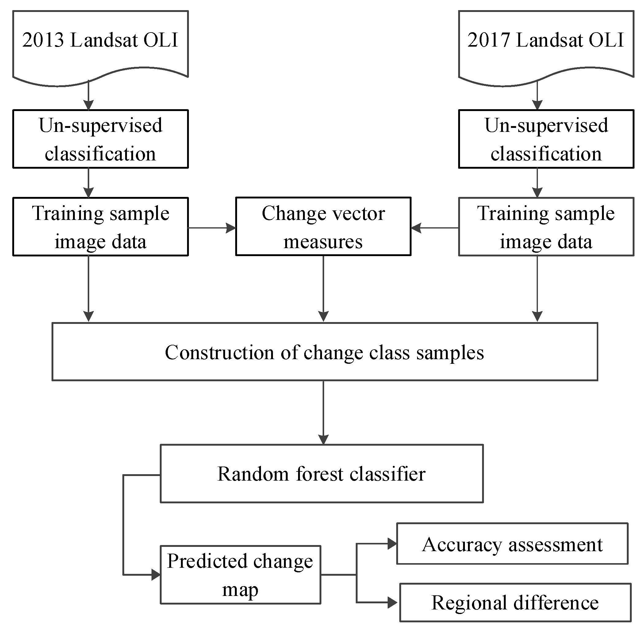
Medium resolution Landsat data support regional monitoring due to their consistent quality, radiometric and spectral resolution [43]. Two cloud free Landsat-8 Operational Land Imager scenes (path/row: 122/44) from 2013 and 2017 were selected for the change analysis with similar seasonal dates (29 November 2013 and 23 November 2017) to reduce phenology effects [4]. The atmospheric-corrected data were obtained through the USGS EarthExplorer and detailed information about this product can be found at https://lta.cr.usgs.gov/L8Level2SR. Six spectral bands were used in the analysis: Blue (0.450 µm–0.515 µm), Green (0.525 µm–0.600 µm), Red (0.630 µm–0.680 µm), Near-infrared (NIR) (0.845 µm–0.885 µm), Short-wavelength infrared 1 (SWIR1) (1.560 µm–1.660 µm) and SWIR2 (2.100 µm–2.300 µm). No atmospheric correction was undertaken because of the unsupervised approach (see detail below). The data were rescaled and the co-registration of the two images was confirmed using a geographic link function in ENVI software (ITT visual information solutions, Boulder, CO, USA).
2.2. Methods Overview
The analysis steps to model and identify changes between 2013 and 2017 from bi-temporal imagery are shown in Figure 2. The process was as follows. First, a series of unsupervised classifications were undertaken using a minimum distance approach with percentage change threshold of 2% and a maximum of 10 iterations. The aim of these was to identify an appropriate classification scheme for this study area. This determined a set of seven classes that could be reliably identified in each image which were then manually labeled. Then, class-to-class training data were selected and labeled automatically with the change classes from the 2013 and 2017 unsupervised classifications. For each class-to-class pair, including no change class pairs, 100 sample locations were selected from within homogenous areas and subjected to a 70/30 training and validation split. From these, the start and end coordinates in six-dimensional image space from the 2013 and 2017 coupled images were determined for each sample and three change vector variables were calculated: magnitude, spectral direction and spectral angle. Thus, the reference samples were labeled with the from-to change classes and contained 15 predictor variables of the six spectral bands for each year and the three derived vector measures. These were used input parameters to a Random Forest classifier to create a predictive model of land cover change. The model was then applied to the combined bi-temporal Landsat images to predict change areas. Finally, regional comparisons were undertaken to compare the magnitude and direction of change in different landscape contexts.
2.3. Land Cover Classes
Iterative investigations of un-supervised classifications confirmed that seven LCLU classes could be identified reliably and repeatably in both images that characterized the mix of land cover and land use in the study area. The seven classes included Low-albedo Impervious Surface (LIS), High-albedo Impervious Surface (HIS), Water (WT), Fishing ponds (FP), Vegetation (VG), Crops (CP), and Bare Soil (BS). These are listed in Table 1 with more detailed descriptions of each class.
It was important that the classification scheme adequately characterized the different land uses in the study area, and one that specifically supported inference about the nature of urban expansion whilst at the same time offered sufficient spectral difference between the classes for them to be reliably identified. As a result, some land covers were split (water and impervious surface) because of their different spectral characteristics associated with different land uses and intensities of land use. For example, HIS has high reflectance because of metal roofs and is commonly found in newly developed suburban areas, whereas LIS is more commonly founded in older urban areas with building materials eroded by air pollution and rain. The difference between WT (water) and FP (fishing ponds) relates to the presence of elements such as vegetation in fishing ponds with the result that the NIR is higher for fishing ponds due to chlorophyll. The difference between VG (vegetation) and CP (crop) relates to the vegetation intensity as recorded in normalized difference vegetation index (NDVI). Vegetation here refers to perennial woody plants or grasses that are not harvested, such that chlorophyll accumulates resulting in a high NDVI. By contrast, crops are harvested annually (sometimes twice) and hence have a lower NDVI value than vegetation.
2.4. From-to Land Cover Changes
Training samples were labeled from the Landsat images and from historical Google Earth images as needed. A false-color combination in RGB (4-5-3) was used to identify the vegetation and water classes. A true color combination in RGB (4-3-2) was used to identify Bare Soil (BS) and to distinguish it from other classes, especially from impervious surface classes. In theory, there are 49 possible class-to-class pairs of change and no-change. Not all of the possible combinations were evaluated. Specifically, because of the aim of understanding urbanization in the Pearl River Delta, changes in impervious surface quality (HIS and LIS), amongst the water classes (WT and FP) and between the vegetation, crop and soil classes were ignored. The 32 class change pairs that were considered are summarized in Table 2.
2.5. Constructing “from-to” Training Samples
The 2012 and 2017 spectral properties of each land cover change sample data were linked together for each training pixel in the form {XBLUE, XGREEN, XRED, XNIR, XSWIR1, XSWIR2, YBLUE, YGREEN, YRED, YNIR, YSWIR1, YSWIR2}, where X and Y refer to 2013 and 2017 data, respectively. For each sample pixel, the distance, magnitude, change vector direction angle and spectral angle were determined from these.
First, the distance d, for each image band pair was calculated:
Then, the magnitude of the change in reflectance intensity ED, was calculated:
There are a number of alternatives for determining change vector direction angle [17,44]. Here, the approach proposed by Bovolo et al. [45] was chosen as in Equation (3) to describe the change vector direction angle (DA):
Finally, the spectral angle mapper (SAM) records the angle between two vectors [46] as described in Equation (4):
where the Xi and Yi represent the spectral information of initial and final stage (2013 and 2017 in this study). ‖ ‖ represents the length of each vector.
After these calculations, the final training samples could be denoted as {XBLUE, XGREEN, XRED, XNIR, XSWIR1, XSWIR2, YBLUE, YGREEN, YRED, YNIR, YSWIR1, YSWIR2, ED, DA, SAM}. Thus, the resulting training data included 12 variables from the Landsat 8 image bands of 2013 and 2017, and the derived change vector variables (direction, angle and the spectral angle). These variables were used to train a Random Forest model.
2.6. Random Forest Classifier
The Random Forest (RF) classifier is an ensemble classifier that uses a set of classification and regression trees to make a predictive model [47]. RF uses training sets to generate multiple (deep) decision trees and have been found to solve some of the problems of over-fitting with other decision trees. When predicting, each tree predicts a result and each result is weighted by the number of votes it receives. The final classification is obtained after some degree of convergence in fitting and majority voting. The number of trees (Ntree) and the number of variables randomly sampled as candidates at each split (Mtry) are two important parameters in the implementation of a RF classifier. The out of bag (OOB) estimate provides a measure of the RF prediction error and an assessment of the accuracy of model. Studies have reported that setting Ntree = 500 is appropriate as the errors are stable around this number [36]. A tuning function in the randomForest R package was used to determine the optimal Mtry parameter. The RF was used to generate a land cover change model. This was then applied to combined 2013 and 2017 image data, plus the three derived vector measures—ED, DA and SAM—to generate a predicated map of land cover change. The accuracy of the RF classification was evaluated using 30% of the reference data samples that were withheld.
2.7. Inter-Regional Analysis
To explore indicative differences in land cover change in different types of regions in the study areas, the ratio of the odds of change between Region 1 and Region 2 was calculated, as described in Comber et al. [42]. These approaches can be used to compare per class differences in change, specific class-to-class changes as well as regional differences. The ratio of change, θ, is as follows:
where θ equals or is near to 1, then change is equally likely in each treatment (region, class, class-to-class change). Essentially, what this approach does is compare the odds of change (i.e., it compares the proportions of change and no change in different study areas (or regions).
3. Results
3.1. RF Classification
The accuracy of the RF classification was undertaken using a 70/30 training and validation split of the reference data. Table 3 shows a correspondence matric of change class errors for the study area. Overall accuracy was found to be 96% which corresponds to the model OOB classification error (4%). Errors were associated with changes between Vegetation to Fishing Ponds (VG and FP) and Crops (CP) with low and high intensity Impervious Surface (LIS and HIS). To confirm the reliability of the approach and because of the out-of-bag error calculated on the training set may not be an unbiased error estimator, a 10-fold cross-validated accuracy measure was determined. In this, the sample is randomly partitioned into 10 equal subsamples and a single subsample is held back as the validation data for each of these. Thus, nine subsamples are each used as training data and then compared with the validation set. The results of doing this indicated a mean value the 10 accuracy measures was 0.964 (with a standard deviation of 0.0009).
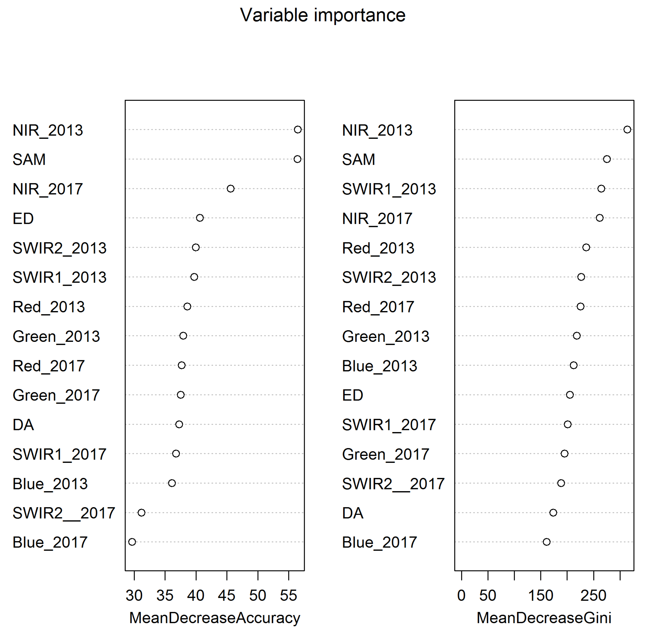
The explanatory power of the input variables was evaluated using Mean Decrease Accuracy and Mean Decrease Gini measures, explained in full in Louppe et al. [48]. In brief, a leave one out cross validation approach is applied to determine the degree to which the inclusion of different variables reduces the error. Figure 3 shows the relative importance of each of the input variables. In this case, NIR in 2013 and SAM alone provide excellent linear separation (Mean Decrease Accuracy), whereas the Mean Decrease Gini plots shows how each variable contributes to the homogeneity of the nodes and leaves in the resulting RF model. Several characteristics are evident: for the spectral bands, NIR band in 2013 had greater explanatory power than visible bands; for the three derived variables, SAM was superior to Euclidean distance and change direction in improving the accuracy and the NIR in 2013 and SAM were found to have almost equal explanatory power; the contribution of other inputs declined linearly except the SWIR2 in 2017 and Blue band in 2017; and SWIR2 in 2017 and Blue in 2017 were not as important as other features.
3.2. Overall Change to Impervious Surface
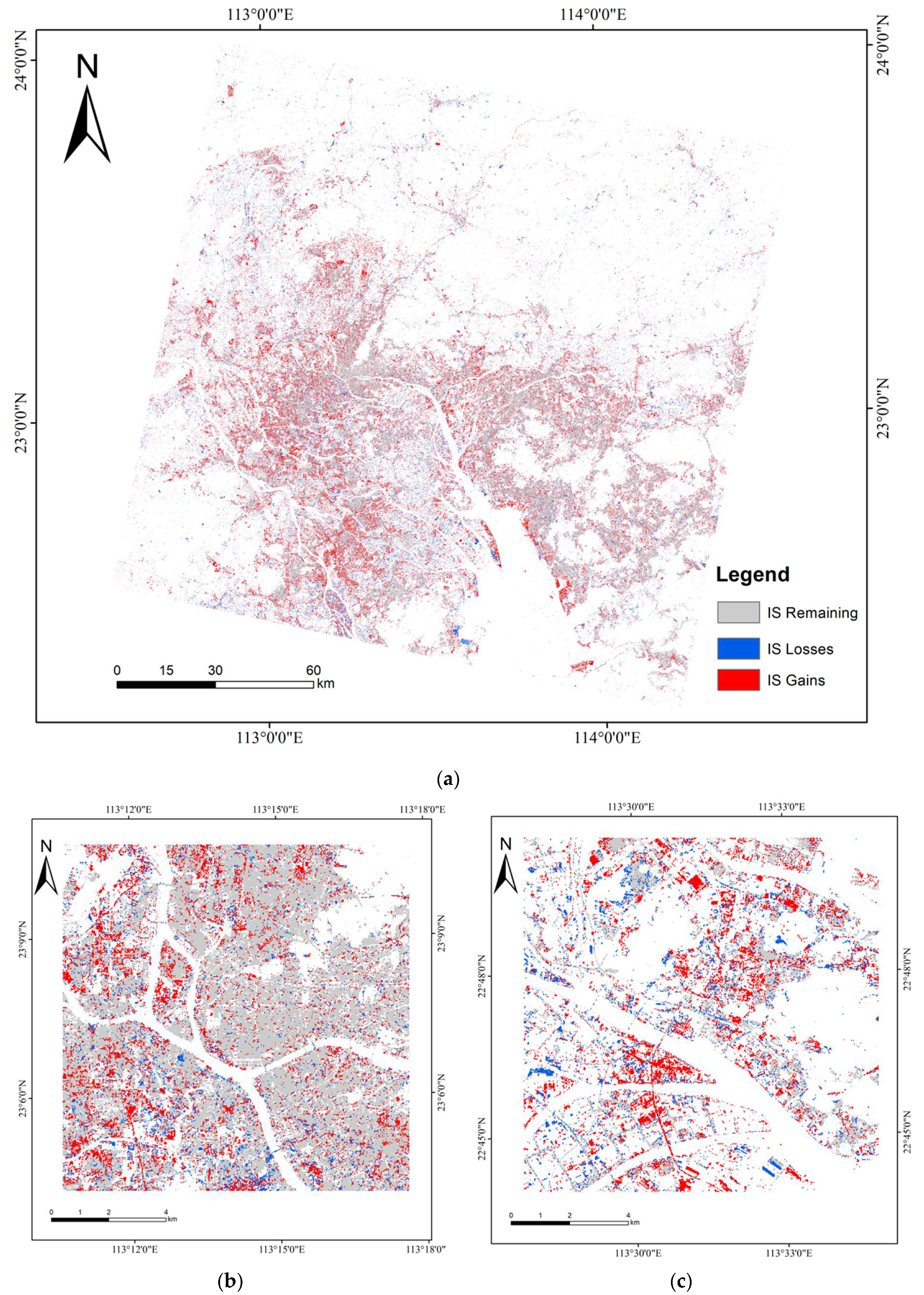
The RF model was then used to predict the LCLU change class for each pixel in the 2013 and 2017 imagery. The result included change and no change classes. Changes to Impervious Surface (IS) [49] provide a critical indicator of urbanization. Changes and no changes to the two IS classes were collapsed and are summarized in Table 4 where the Loss value indicates the amount of IS in 2013 that changed to another class in 2017 and the Gain value indicates the amount of IS in 2017 that was a different class in 2013. The unchanged remaining IS area was found to be 2957.8 km2, the gains to IS were 1502.4 km2 and the losses were 757.3 km2. The locales of IS change (loses and gains) and no change are mapped in Figure 4. The unchanged areas are found mostly in the core urban areas with the gains found mostly in the peri-urban area around the urban fringe, as would be expected.
3.3. Per Class. Changes to/from Impervious Surface
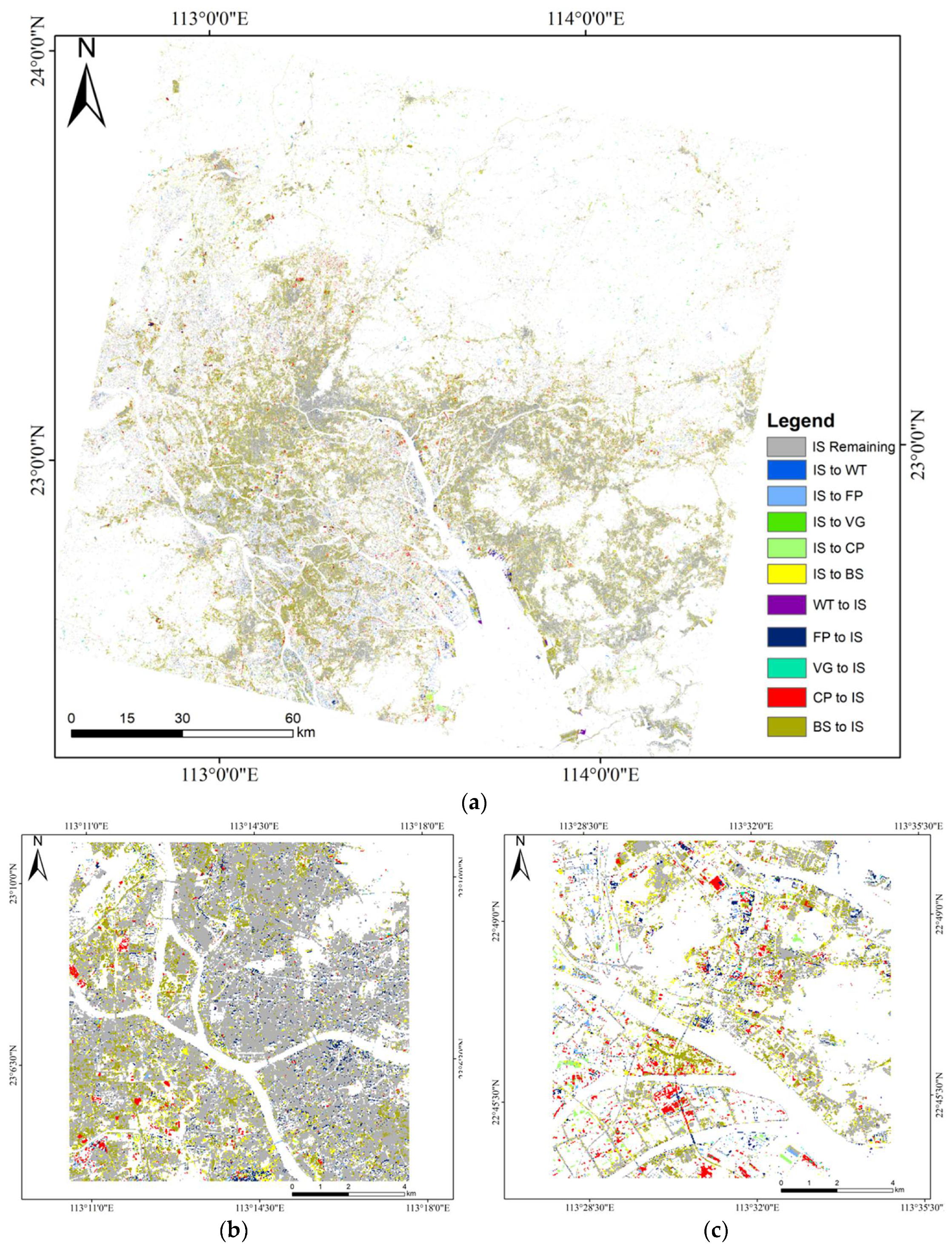
Detailed land cover changes are shown in Figure 5 and summarized in Table 5. The most common loss was found between Impervious Surface (LIS and HIS) and Bare Soil (BS), fishing ponds (FP) and crops (CP). In Region 1, an area located near the urban center characterized by high-density settlements and buildings, the rate of land cover changes was high (Figure 4b and Figure 5b). In Region 2, an area with high levels of agricultural activity near the Pearl River estuary (Figure 4c and Figure 5c), the rate of land cover changes was also high, but mainly found in the margins of unchanged agricultural land.
The overall prediction accuracies for impervious surface related changes are shown in Table 5 and the likely error directions are indicated in Table 3. For LCLU transitions involving Impervious Surfaces classes, the accuracy was around 0.95, with some classes showing lower overall accuracy rates: CP to HIS, LIS to FP, and FP to LIS which were 0.87 and 0.90, 0.93, respectively.
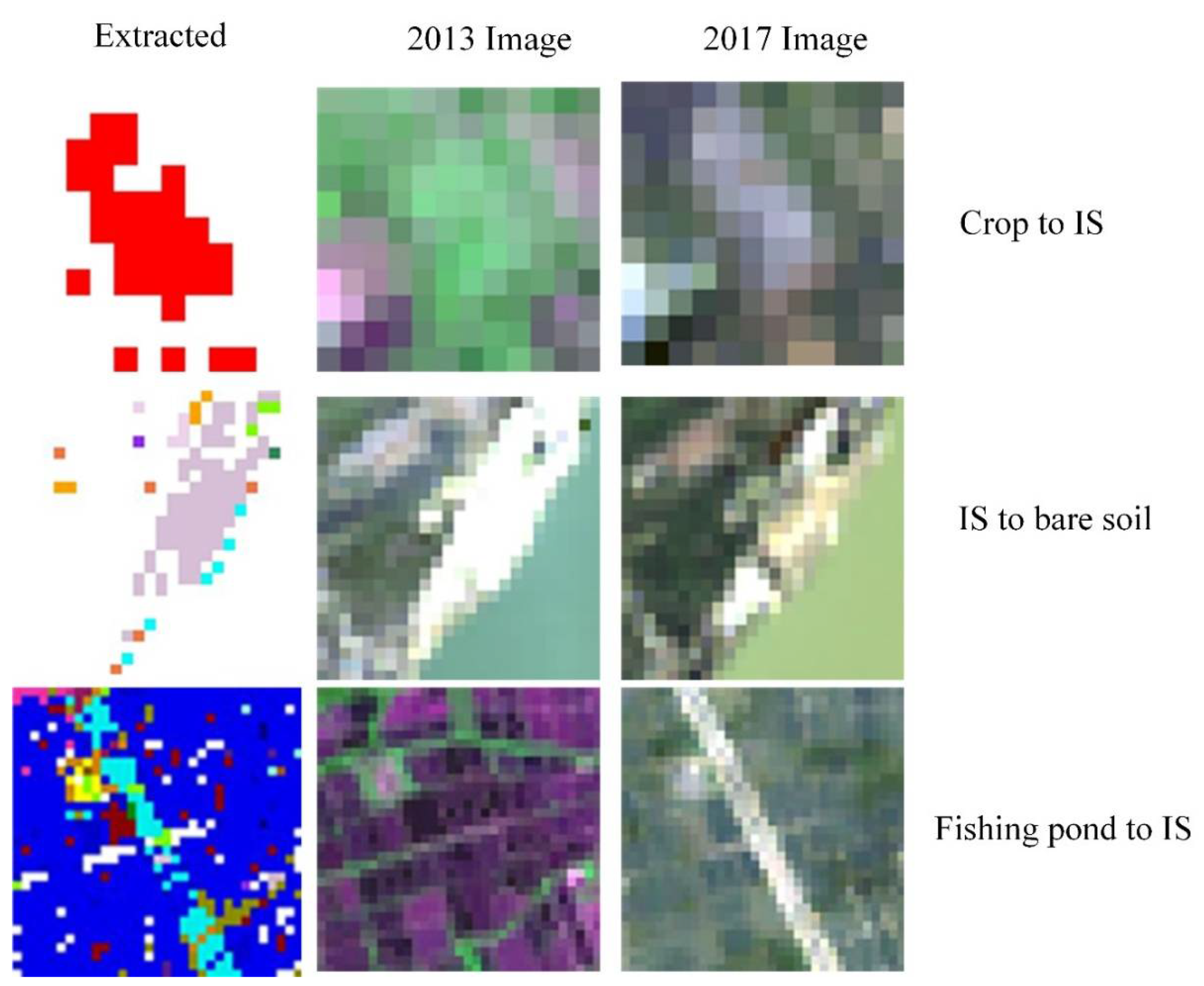
Figure 6 shows detail of some example areas. These changes are typical of the transitions observed in the study areas: from crop to IS as development occurs, from fishing pond to IS as development (in this case a road) in agricultural areas, and from IS to Bare Soil. The latter transition is counter to other findings which have suggested the development permanency of IS once established (e.g., [50]). However, in reality, rapid urban functional change does occur under development scenarios in dynamic urban environments.
3.4. Inter.-Region Analysis of Region 1 and Region 2
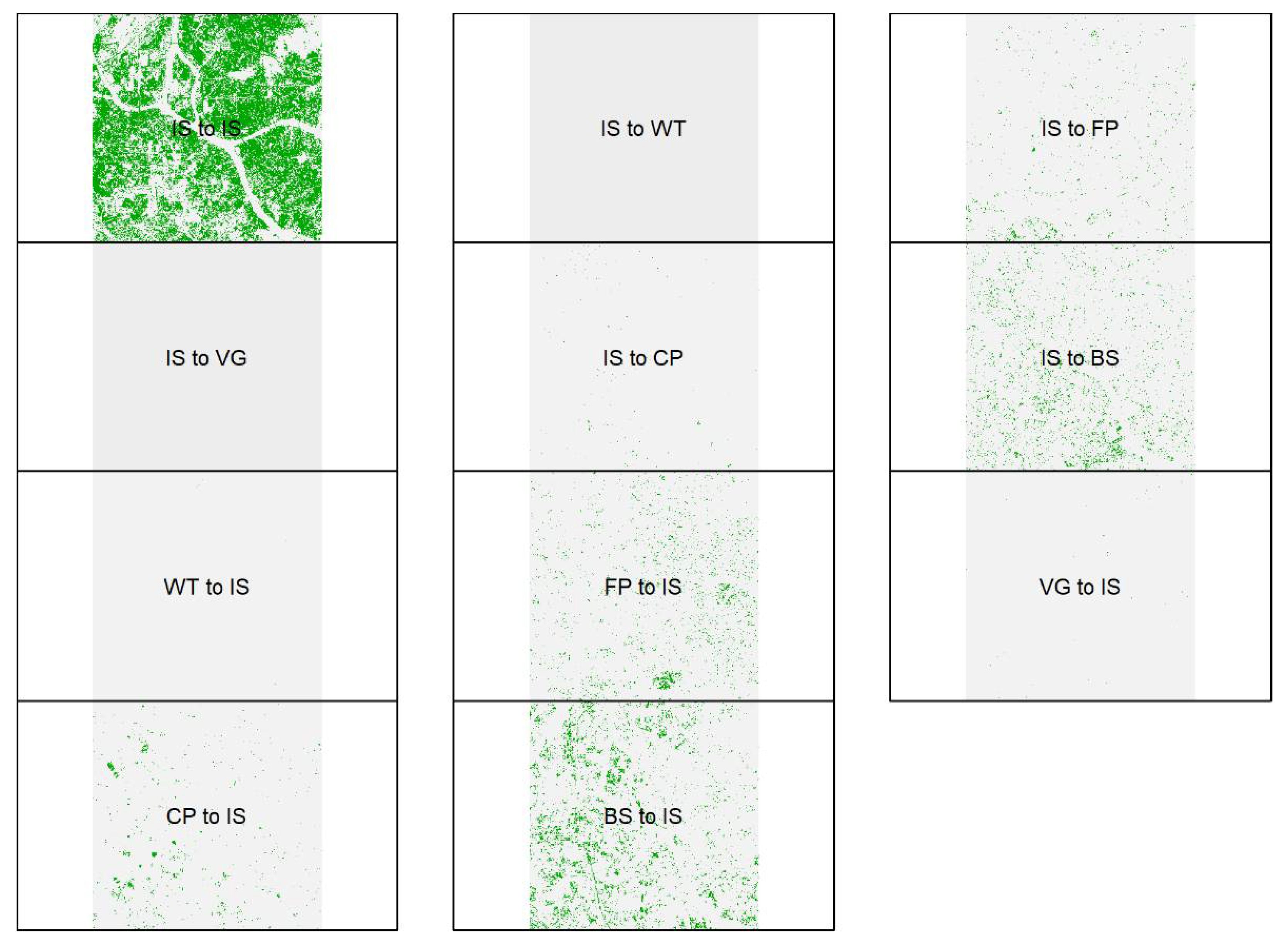
Region 1 was characterized by high density settlements located in the core urban area. The distribution of land cover changes in Region 1 are shown in Figure 7. The dominant LCLU type was IS (the two classes LIS and HIS are collapsed for the remainder of the results), most of which remained unchanged. The large-scale changes are between IS and BS (both losses and gains). More generally, the distribution of IS from agriculture were mostly located at the outer edge of the city regions. The area of water related classes has not changed much in his region.
Table 6 quantifies the LCLU transitions in Region 1. This region is dominated by IS, with 49% of the area remaining unchanged. There are much fewer losses to IS than gains, fewer changes to and from natural land covers such as Water (WT) and Vegetation (VG) and much greater changes to and from agricultural types such as Fishing Ponds (FP) and Crop (CP), associated with development: the gains in IS gains are conversions from Water, Fishing Ponds, Vegetation and Crops and there are also intra-class changes between LIS and HIS which are not shown here.
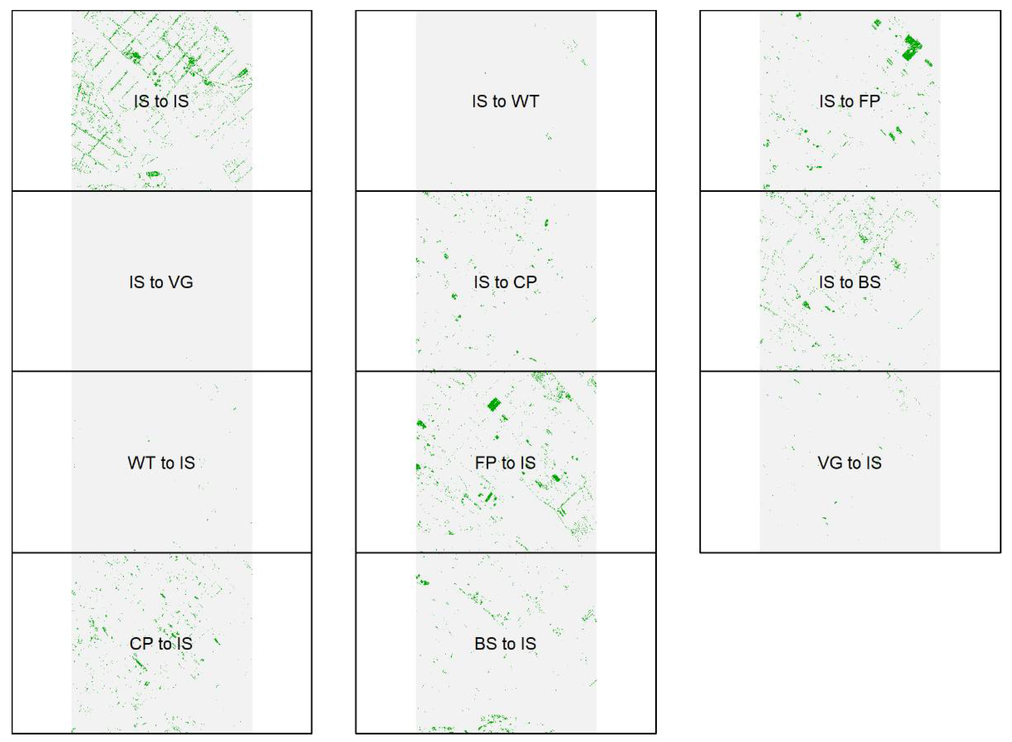
The distribution of land cover changes for Region 2 are shown in Figure 8. Region 2 is characterized by high levels of agricultural activity (Fishing Ponds and crop classes) and is located in the peri-urban area. Such regions contain distributed human settlements. The changes between IS with Crops and Fishing Pond dominated this region. The conversions from agriculture types demonstrate that impact of human settlement in this region, despite it being more rural in character. These changes are also indicated in Table 6, which quantifies the IS gains from Fishing Ponds, vegetation, and crops, and also shows that IS is converted to other LCLU types. This may be indicative of a misclassification in this region between IS and Bare Soil due to their spectral similarity and a potential overestimation of IS.
It is also possible to quantify the regional differences in the probability of different changes using relative odds ratios [42]. The relative likelihood of change to IS from any land cover class was 6.7 times more likely in Region 2 (peri-urban) than in Region 1 (urban). Although seemingly counter-intuitive, gross changes in the peri-urban region are more likely because in urban region have already been developed (i.e., already contain much Impervious Surface) and further changes to that class are regulated by local government and municipal authorities. There are fewer regulations in agricultural regions and much more freedom for individual land owners to develop the land if they wish. Further comparison of the differences in the relative likelihood of IS losses and gains are shown in Table 7. This shows that, for example, the likelihood of change from IS to FP is 3.07 greater (0.326−1) times in Region 2 than in Region 1. In general, losses from IS and gains to IS are more likely in Region 1 than in Region 2, except for losses to and gains from Bare Soil (BS).
4. Discussion
This paper describes a modified change vector analysis approach for quantifying land cover change in bi-temporal data that combines direct multi-date classification [5] with CVA measures (magnitude, spectral direction and spectral angle) and image band reflectance values, and uses these to train a Random Forest model of LCLU change. The method has not sought to identify change vectors or land cover classes at either Time 1 (2013) or Time 2 (2017). Rather, it used the bi-temporal image properties of labeled class-to-class transitions, with measures derived from the change vector (Euclidian Distance, change vector Direction Angle and Spectral Angle Mapper) to train a Random Forest classifier. The samples were automatically created from a supervised classification of Landsat images at both dates that generated seven classes, which were manually labeled. The results are promising, with high accuracies and the method provides an intuitive and quick way of quantifying the patterns of urban growth and change that is of use to planners and policy makers who frequently want to quantify and locate land cover/land use changes. The approach circumvents the problems associated with post classification change [19] and does not require the technological, data and infrastructure resources described in [7], although it operates under a similar philosophy: the identification of change is the primary aim before updating the baseline. This paper has not sought to update any baseline.
The method is sensitive to the reliability of the unsupervised classification. Reference data were selected from within homogenous areas to avoid edge and bi-temporal image mis-registration effects. Some degree of automated reference data generation is needed simply because of dimensionality imposed by trying to characterize transitions rather than start and end vectors: here, a seven-class nomenclature was used (49 transitions) but it is not uncommon for land cover initiatives to have 12–20 classes (144–400 transition classes).
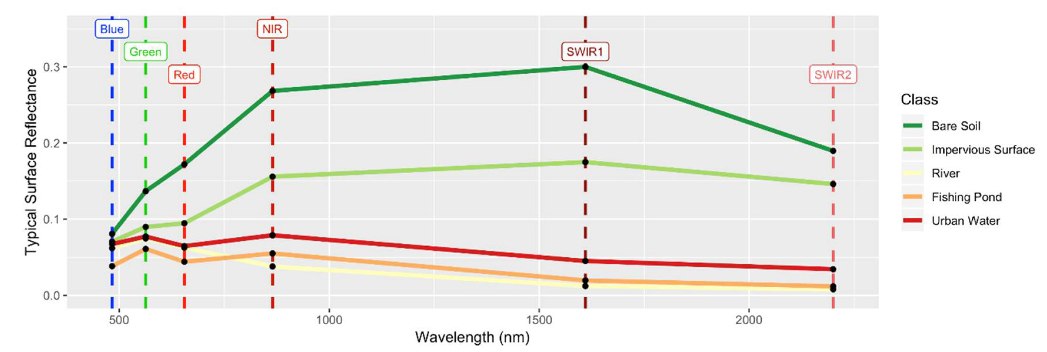
There are a number of areas of further work. First, this study considered bi-temporal data, providing a snapshot of urban land use changes between two time periods. The analysis of multi-temporal image data to provide a series of snapshots of change, covering both annual census dates and seasonal changes, would support the investigation of specific urban processes such as urban sprawl, landscape fragmentation and changes in land use diversity. Further, by considering different regions, as was done here using the methods described in [42], local variations in these processes can be quantified. Second, different model selection approaches will be investigated to determine which variables to include for specific types of change. Here, all of the variables were included as potential descriptors (predictors) of change and Figure 4 provides an indication of the relative utility of different variables in this study. For example, during the reference data collection process, some water bodies in urban regions (“Urban Water”) were labeled as Water, but may have been Fishing Ponds; Region 2 was dominated by agriculture related types (Crops and Fishing Ponds) and here misclassifications were found between Bare Soil and IS due to the similarity of their spectral characters. Typical spectral values are shown in Figure 9 and illustrate the potential for these confusions. Hyperspectral images, especially with high spectral information in SWIR bands, may be a solution to this problem. Third, the method will be applied and evaluated in other environments, using different data, to further investigate the potential applicability and limitations of the approach. It will be applied to multi-temporal reference data to support analyses of the processes associated with changes land use in a large regional analysis in the Loess Plateau, China, using MODIS data. The aim here will be to quantify the coupled relationships between soil–water processes and multi-scale agro-ecosystem LCLU changes to evaluate the impacts on landscape re-greening and restoration agricultural sustainability initiatives. Finally, a further extension to this work is to examine fuzzy land cover class transitions [51,52]. Conceptualizing change classes in this way, based on a fuzzy sets approach, would require second order vagueness to be accommodated rather than a crisp, Boolean concept of change. This may address some of the sub-pixel issues associated with urban impervious surface estimation and working with medium resolution satellite imagery. Vague land cover change analysis could allow different memberships to the set of “change” to be explored, either globally or on a per change class basis. Finally, many large-scale operational monitoring initiatives use a sequence of change signals to generate increasingly confirmatory evidence to support a hypothesis of object level change. Such evidence could be included in the model specification by passing lagged image variables for Time 1 to Time n into the classification algorithm rather than data from just two scenes.
5. Conclusions
This analysis used information from bi-temporal imagery and change vectors to train a Random Forest classifier, combining processes driven monitoring approaches being adopted by large national inventories [7] and direct multi-date classification or multi-date direct comparison approaches [5,8]. It developed predictive models of LCLU change and no change from training data sampled from manually labeled unsupervised classifications of remote sensing data. These were used as inputs to a supervised change model to generate a surface of predicted class-to-class changes and no change. Odds ratios were used to quantify inter-regional differences in LCLU change. The results indicate that change vector derived variables (distance, direction angle and Spectral Angle Mapper) along with bi-temporal image spectral properties provide a useful short-cut to accurate change detection. This approach supports effective and informative analyses of LCLU change able to support policy and planning in rapidly changing environments such as those experiencing urbanization. It is conceptually elegant and can be very quickly applied, supporting the rapid generation of LCLU change data to support policy.
Author Contributions
Conceptualization, A.C.; Methodology, A.C., Y.L. (Ying Luo), Y.R. and R.X.; Software, R.X.; Validation, R.X. and A.C.; Formal Analysis, R.X.; Investigation, R.X.; Resources, R.X. and H.L.; Data Curation, R.X.; Writing—Original Draft Preparation, A.C. and R.X.; Writing—Review and Editing, R.X., and A.C.; Visualization, R.X.; Supervision, H.L., Y.L. (Yihe Lü) and A.C.; Project Administration, H.L. and Y.L. (Yihe Lü); and Funding Acquisition, A.C., Y.L. (Yihe Lü) and H.L.
Funding
This research was supported by the National Key Basic Research Program of China (2015CB954103), the Collaborative Innovation Center for Major Ecological Security Issues of Jiangxi Province and Monitoring Implementation (No. JXS-EW-00) and the China-UK collaborative research on critical zone science funded by the Natural Environment Research Council (NERC) Newton Fund (NE/N007433/1) and National Natural Science Foundation of China (NSFC) (No. 41571130083).
Acknowledgments
The authors would like thank the anonymous reviewers whose suggestions greatly improved this manuscript.
Conflicts of Interest
The authors declare no conflict of interest. The founding sponsors had no role in the design of the study; in the collection, analyses, or interpretation of data; in the writing of the manuscript, and in the decision to publish the results.
References
- Gatrell, J.D.; Jensen, R.R. Sociospatial applications of remote sensing in urban environments. Geogr. Compass 2008, 2, 728–743. [Google Scholar] [CrossRef]
- Turner, B.L.; Lambin, E.F.; Reenberg, A. The emergence of land change science for global environmental change and sustainability. Proc. Nat. Acad. Sci. USA 2007, 104, 20666–20671. [Google Scholar] [CrossRef] [PubMed] [Green Version]
- Lambin, E.F.; Strahlers, A.H. Change-vector analysis in multitemporal space: A tool to detect and categorize land-cover change processes using high temporal-resolution satellite data. Remote Sens. Environ. 1994, 48, 231–244. [Google Scholar] [CrossRef]
- Lu, D.; Mausel, P.; Brondizio, E.; Moran, E. Change detection techniques. Int. J. Remote Sens. 2004, 25, 2365–2401. [Google Scholar] [CrossRef]
- Bruzzone, L.; Serpico, S.B. An iterative technique for the detection of land-cover transitions in multitemporal remote-sensing images. IEEE Trans. Geosci. Remote Sens. 1997, 35, 858–867. [Google Scholar] [CrossRef]
- Zhu, Z.; Woodcock, C.E. Continuous change detection and classification of land cover using all available Landsat data. Remote Sens. Environ. 2014, 144, 152–171. [Google Scholar] [CrossRef]
- White, J.C.; Wulder, M.A.; Hermosilla, T.; Coops, N.C.; Hobart, G.W. A nationwide annual characterization of 25years of forest disturbance and recovery for Canada using Landsat time series. Remote Sens. Environ. 2017, 194, 303–321. [Google Scholar] [CrossRef]
- Hussain, M.; Chen, D.; Cheng, A.; Wei, H.; Stanley, D. Change detection from remotely sensed images: From pixel-based to object-based approaches. ISPRS J. Photogramm. 2013, 80, 91–106. [Google Scholar] [CrossRef]
- Tewkesbury, A.P.; Comber, A.J.; Tate, N.J.; Lamb, A.; Fisher, P.F. A critical synthesis of remotely sensed optical image change detection techniques. Remote Sens. Environ. 2015, 160, 1–14. [Google Scholar] [CrossRef] [Green Version]
- Zhu, Z. Change detection using Landsat time series: A review of frequencies, preprocessing, algorithms, and applications. ISPRS J. Photogramm. 2017, 130, 370–384. [Google Scholar] [CrossRef]
- Coulter, L.L.; Hope, A.S.; Stow, D.A.; Lippitt, C.D.; Lathrop, S.J. Time–space radiometric normalization of TM/ETM+ images for land cover change detection. Int. J. Remote Sens. 2011, 32, 7539–7556. [Google Scholar] [CrossRef]
- Peiman, R. Pre-classification and post-classification change-detection techniques to monitor land-cover and land-use change using multi-temporal Landsat imagery: A case study on Pisa Province in Italy. Int. J. Remote Sens. 2011, 32, 4365–4381. [Google Scholar] [CrossRef]
- Carvalho Júnior, O.A.; Guimarães, R.F.; Gillespie, A.R.; Silva, N.C.; Gomes, R.A. A new approach to change vector analysis using distance and similarity measures. Remote Sens. 2011, 3, 2473–2493. [Google Scholar] [CrossRef]
- Thonfeld, F.; Feilhauer, H.; Braun, M.; Menz, G. Robust Change Vector Analysis (RCVA) for multi-sensor very high resolution optical satellite data. Int. J. Appl. Earth Obs. 2016, 50, 131–140. [Google Scholar] [CrossRef]
- Dewan, A.M.; Yamaguchi, Y. Land use and land cover change in Greater Dhaka, Bangladesh: Using remote sensing to promote sustainable urbanization. Appl. Geogr. 2009, 29, 390–401. [Google Scholar] [CrossRef]
- Yuan, F.; Sawaya, K.E.; Loeffelholz, B.C.; Bauer, M.E. Land cover classification and change analysis of the Twin Cities (Minnesota) Metropolitan Area by multitemporal Landsat remote sensing. Remote Sens. Environ. 2005, 98, 317–328. [Google Scholar] [CrossRef]
- Michalek, J.L.; Wagner, T.W.; Luczkovich, J.J.; Stoffle, R.W. Multispectralchange vector analysis for monitoring coastal marine environments. Photogramm. Eng. Remote Sens. 1993, 59, 381–384. [Google Scholar]
- Coppin, P.; Jonckheere, I.; Nackaerts, K.; Muys, B.; Lambin, E. Digital change detection methods in ecosystem monitoring: A review. Int. J. Remote Sens. 2004, 25, 1565–1596. [Google Scholar] [CrossRef]
- Fuller, R.M.; Smith, G.M.; Devereux, B.J. The characterisation and measurement of land cover change through remote sensing: Problems in operational applications? Int. J. Appl. Earth Obs. Geoinf. 2003, 4, 243–253. [Google Scholar] [CrossRef]
- Serra, P.; Pons, X.; Sauri, D. Post-classification change detection with data from different sensors: Some accuracy considerations. Int. J. Remote Sens. 2003, 24, 3311–3340. [Google Scholar] [CrossRef]
- Comber, A.; Kuhn, W. Fuzzy difference and data primitives: A transparent approach for supporting different definitions of forest in the context of REDD+. Geogr. Helv. 2018, 73, 151–163. [Google Scholar] [CrossRef]
- Loveland, T.R.; Dwyer, J.L. Landsat: Building a strong future. Remote Sens. Environ. 2012, 122, 22–29. [Google Scholar] [CrossRef]
- Gómez, C.; White, J.C.; Wulder, M.A. Optical remotely sensed time series data for land cover classification: A review. ISPRS J. Photogramm. 2016, 116, 55–72. [Google Scholar] [CrossRef]
- Hermosilla, T.; Wulder, M.A.; White, J.C.; Coops, N.C.; Hobart, G.W. Disturbance-Informed Annual Land Cover Classification Maps of Canada’s Forested Ecosystems for a 29-Year Landsat Time Series. Can. J. Remote Sens. 2018, 44, 1–21. [Google Scholar] [CrossRef]
- Gauld, J.H.; Bell, J.S.; Towers, W.; Miller, D.R. The Measurement and Analysis of Land Cover Changes in the Cairngorms; MLURI: Aberdeen, UK, 1991. [Google Scholar]
- Comber, A.; Davies, H.; Pinder, D.; Whittow, J.B.; Woodhall, A.; Johnson, S.C.M. Mapping coastal land use changes 1965–2014: Methods for handling historical thematic data. Trans. Inst. Br. Geogr. 2016, 41, 442–459. [Google Scholar] [CrossRef]
- Fisher, P. The pixel: A snare and a delusion. Int. J. Remote Sens. 1997, 18, 679–685. [Google Scholar] [CrossRef]
- Wulder, M.A.; White, J.C.; Loveland, T.R.; Woodcock, C.E.; Belward, A.S.; Cohen, W.B.; Fosnight, E.A.; Shaw, J.; Masek, J.G.; Roy, D.P. The global Landsat archive: Status, consolidation, and direction. Remote Sens. Environ. 2016, 185, 271–283. [Google Scholar] [CrossRef]
- Gorelick, N.; Hancher, M.; Dixon, M.; Ilyushchenko, S.; Thau, D.; Moore, R. Google Earth Engine: Planetary-scale geospatial analysis for everyone. Remote Sens. Environ. 2017, 202, 18–27. [Google Scholar] [CrossRef]
- Lewis, A.; Oliver, S.; Lymburner, L.; Evans, B.; Wyborn, L.; Mueller, N.; Raevksi, G.; Hooke, J.; Woodcock, R.; Sixsmith, J.; et al. The Australian geoscience data cube—Foundations and lessons learned. Remote Sens. Environ. 2017, 202, 276–292. [Google Scholar] [CrossRef]
- Malila, W.A. Change Vector Analysis: An Approach for Detecting Forest Changes with Landsat, in Symposium. Available online: https://docs.lib.purdue.edu/cgi/viewcontent.cgi?article=1386&context=lars_symp (accessed on 19 July 2018).
- Bovolo, F.; Bruzzone, L. A theoretical framework for unsupervised change detection based on change vector analysis in the polar domain. IEEE Trans. Geosci. Remote Sens. 2007, 45, 218–236. [Google Scholar] [CrossRef]
- Bruzzone, L.; Prieto, D.F. Automatic analysis of the difference image for unsupervised change detection. IEEE Trans. Geosci. Remote Sens. 2000, 38, 1171–1182. [Google Scholar] [CrossRef]
- Xian, G.; Homer, C. Updating the 2001 National Land Cover Database impervious surface products to 2006 using Landsat imagery change detection methods. Remote Sens. Environ. 2010, 114, 1676–1686. [Google Scholar] [CrossRef]
- Bovolo, F.; Marchesi, S.; Bruzzone, L. A framework for automatic and unsupervised detection of multiple changes in multitemporal images. IEEE Trans. Geosci. Remote Sens. 2012, 50, 2196–2212. [Google Scholar] [CrossRef]
- Lawrence, R.L.; Wood, S.D.; Sheley, R.L. Mapping invasive plants using hyperspectral imagery and Breiman Cutler classifications (RandomForest). Remote Sens. Environ. 2006, 100, 356–362. [Google Scholar] [CrossRef]
- Allen, T.R.; Kupfer, J.A. Application of spherical statistics to change vector analysis of Landsat data: Southern Appalachian spruce–fir forests. Remote Sens. Environ. 2000, 74, 482–493. [Google Scholar] [CrossRef]
- Cohen, W.B.; Fiorella, M.; Gray, J.; Helmer, E.; Anderson, K. An efficient and accurate method for mapping forest clearcuts in the Pacific Northwest using Landsat imagery. Photogramm. Eng. Remote Sens. 1998, 64, 293–299. [Google Scholar]
- Johnson, R.D.; Kasischke, E.S. Change vector analysis: A technique for the multispectral monitoring of land cover and condition. Int. J. Remote. Sens. 1998, 19, 411–426. [Google Scholar] [CrossRef]
- Nackaerts, K.; Vaesen, K.; Muys, B.; Coppin, P. Comparative performance of a modified change vector analysis in forest change detection. Int. J. Remote. Sens. 2005, 26, 839–852. [Google Scholar] [CrossRef] [Green Version]
- Richards, J.A. Remote Sensing Digital Image Analysis; Springer: Berlin, Germany, 1993. [Google Scholar]
- Comber, A.; Balzter, H.; Cole, B.; Johnson, S.; Oguto, B.; Fisher, P. Methods to quantify regional differences in land cover change. Remote Sens. 2016, 8, 176. [Google Scholar] [CrossRef]
- Vogelmann, J.E.; Gallant, A.L.; Shi, H.; Zhu, Z. Perspectives on monitoring gradual change across the continuity of Landsat sensors using time-series data. Remote Sens. Environ. 2016, 185, 258–270. [Google Scholar] [CrossRef]
- Chen, J.; Gong, P.; Chunyang, H.; Pu, R.; Shi, P. Land-use/land-cover change detection using improved change-vector analysis. Photogramm. Eng. Remote Sens. 2003, 69, 369–379. [Google Scholar] [CrossRef]
- Bovolo, F.; Marchesi, S.; Bruzzone, L. A nearly lossless 2D representation and characterization of change information in multispectral images. In Proceedings of the IEEE International Geoscience and Remote Sensing Symposium, Honolulu, HI, USA, 25–30 July 2010; pp. 3074–3077. [Google Scholar]
- Kruse, F.A.; Lefkoff, A.B.; Boardman, J.W.; Heidebrecht, K.B.; Shapiro, A.T.; Barloon, P.J.; Goetz, A.F.H. The spectral image processing system (SIPS)—Interactive visualization and analysis of imaging spectrometer data. Remote Sens. Environ. 1993, 44, 145–163. [Google Scholar] [CrossRef]
- Breiman, L. Random forests. Mach. Learn. 2001, 45, 5–32. [Google Scholar] [CrossRef]
- Louppe, G.; Wehenkel, L.; Sutera, A.; Geurts, P. Understanding variable importances in forests of randomized trees. In Proceedings of the 26th Neural Information Processing Systems Conference, Lake Tahoe, NV, USA, 5–8 December 2013. [Google Scholar]
- Slonecker, E.T.; Jennings, D.B.; Garofalo, D. Remote sensing of impervious surfaces: A review. Remote Sens. Rev. 2001, 20, 227–255. [Google Scholar] [CrossRef]
- Schneider, A.; Mertes, C.M. Expansion and growth in Chinese cities, 1978–2010. Environ. Res. Lett. 2014, 9, 024008. [Google Scholar] [CrossRef] [Green Version]
- Fisher, P.; Arnot, C.; Wadsworth, R.; Wellens, J. Detecting change in vague interpretations of landscapes. Ecol. Inf. 2006, 1, 163–178. [Google Scholar] [CrossRef] [Green Version]
- Fisher, P.F. Remote sensing of land cover classes as type 2 fuzzy sets. Remote Sens. Environ. 2010, 114, 309–321. [Google Scholar] [CrossRef]
Figure 1.
(a) The study area of the Pearl River Delta with Landsat 8 imagery for 2017 (in Red (band 4), Green (band 3), Blue (band 2) true color composites) and 2 sub-regions indicated in red (Region 1) and blue (Region 2), respectively. The two sub-regions (b) Region 1 and (c) Region 2 are shown in true color.

Figure 2.
The flowchart of the methods applied in this study.

Figure 3.
The relative importance of each variable as indicated by Mean Decrease Accuracy and Mean Decrease Gini measures.
Figure 3.
The relative importance of each variable as indicated by Mean Decrease Accuracy and Mean Decrease Gini measures.

Figure 4.
(a) The overall map of change and no-change (in white) for Impervious Surface; (b) detail in Region 1; and (c) detail in Region 2.
Figure 4.
(a) The overall map of change and no-change (in white) for Impervious Surface; (b) detail in Region 1; and (c) detail in Region 2.

Figure 5.
(a) The overall map of Impervious Surface change; (b) detail in Region; and (c) detail in Region 2.
Figure 5.
(a) The overall map of Impervious Surface change; (b) detail in Region; and (c) detail in Region 2.

Figure 6.
Examples of typical transitions to and from Impervious Surface.

Figure 7.
Impervious Surface related land changes in Region 1.

Figure 8.
Change map of Region 2.

Figure 9.
Typical spectral characteristics of different LCLU classes.


Table 1.
Land cover classification scheme in this study.
| Class Label | Description |
|---|---|
| HIS | Impervious surface with high reflectance, including metal roofs, new concrete road. |
| LIS | Impervious surface with low reflectance, including old concrete road, asphalt road etc. |
| WT | Water, including reservoirs, main river channels. |
| FP | Fishing ponds, artificial frequently with fishes and/or vegetation. |
| CP | Crops and vegetation with low NDVI. |
| VG | Vegetation with woody plant (trees, shrubs, or lianas) and perennial grasses. |
| BS | Bare soil surface devoid of any plant material. |
Table 2.
The “from-to” land cover change matrix (IS, impervious surface; WT, water; FP, fishing ponds; VG, vegetation; CP, crop; BS, bare soil).
Table 2.
The “from-to” land cover change matrix (IS, impervious surface; WT, water; FP, fishing ponds; VG, vegetation; CP, crop; BS, bare soil).
| Initial Class (from 2013) | Final Class (to 2017) | |||||||
|---|---|---|---|---|---|---|---|---|
| HIS | LIS | WT | FP | VG | CP | BS | ||
| HIS | X | X | X | X | X | |||
| LIS | X | X | X | X | X | |||
| WT | X | X | X | X | X | |||
| FP | X | X | X | X | X | |||
| VG | X | X | X | X | ||||
| CP | X | X | X | X | ||||
| BS | X | X | X | X | ||||
Table 3.
The correspondence matrix of observed change classes (rows) and predicted change class (columns).
Table 3.
The correspondence matrix of observed change classes (rows) and predicted change class (columns).
| LIS-WT | LIS-FP | LIS-VG | LIS-CP | LIS-BS | HIS-WT | HIS-FP | HIS-VG | HIS-CP | HIS-BS | WT-LIS | WT-HIS | WT-VG | WT-CP | WT-BS | FP-LIS | FP-HIS | FP-VG | FP-CP | FP-BS | VG-LIS | VG-HIS | VG-WT | VG-FP | CP-LIS | CP-HIS | CP-WT | CP-FP | BS-LIS | BS-HIS | BS-WT | BS-FP | |
|---|---|---|---|---|---|---|---|---|---|---|---|---|---|---|---|---|---|---|---|---|---|---|---|---|---|---|---|---|---|---|---|---|
| LIS-WT | 28 | 2 | ||||||||||||||||||||||||||||||
| LIS-FP | 28 | |||||||||||||||||||||||||||||||
| LIS-VG | 30 | |||||||||||||||||||||||||||||||
| LIS-CP | 29 | 1 | ||||||||||||||||||||||||||||||
| LIS-BS | 30 | |||||||||||||||||||||||||||||||
| HIS-WT | 30 | |||||||||||||||||||||||||||||||
| HIS-FP | 1 | 29 | ||||||||||||||||||||||||||||||
| HIS-VG | 30 | |||||||||||||||||||||||||||||||
| HIS-CP | 30 | |||||||||||||||||||||||||||||||
| HIS-BS | 30 | |||||||||||||||||||||||||||||||
| WT-LIS | 30 | |||||||||||||||||||||||||||||||
| WT-HIS | 30 | |||||||||||||||||||||||||||||||
| WT-VG | 30 | |||||||||||||||||||||||||||||||
| WT-CP | 30 | |||||||||||||||||||||||||||||||
| WT-BS | 30 | |||||||||||||||||||||||||||||||
| FP-LIS | 2 | 28 | ||||||||||||||||||||||||||||||
| FP-HIS | 29 | |||||||||||||||||||||||||||||||
| FP-VG | 1 | 29 | ||||||||||||||||||||||||||||||
| FP-CP | 1 | 29 | ||||||||||||||||||||||||||||||
| FP-BS | 1 | 29 | ||||||||||||||||||||||||||||||
| VG-LIS | 28 | 2 | ||||||||||||||||||||||||||||||
| VG-HIS | 25 | 5 | ||||||||||||||||||||||||||||||
| VG-WT | 29 | 1 | ||||||||||||||||||||||||||||||
| VG-FP | 24 | 6 | ||||||||||||||||||||||||||||||
| CP-LIS | 1 | 27 | 2 | |||||||||||||||||||||||||||||
| CP-HIS | 3 | 27 | ||||||||||||||||||||||||||||||
| CP-WT | 30 | |||||||||||||||||||||||||||||||
| CP-FP | 1 | 2 | 27 | |||||||||||||||||||||||||||||
| BS-LIS | 2 | 28 | ||||||||||||||||||||||||||||||
| BS-HIS | 30 | |||||||||||||||||||||||||||||||
| BS-WT | 30 | |||||||||||||||||||||||||||||||
| BS-FP | 30 |
Table 4.
The total area of changed and un-changed Impervious Surface in km2.
| Change Area: Loss | Change Area: Gain | Remaining (No-Change) |
|---|---|---|
| 757.3 | 1502.4 | 2957.8 |
Table 5.
Area and accuracy of each changed class (IS-related only).
| Loss Class | Area (km2) | Accuracy | Gain Class | Area (km2) | Accuracy |
|---|---|---|---|---|---|
| HIS to WT | 3.51 | 0.98 | WT to LIS | 4.29 | 0.97 |
| HIS to FP | 150.75 | 0.98 | WT to HIS | 5.87 | 1.00 |
| HIS to VG | 20.57 | 1.00 | FP to LIS | 26.61 | 0.93 |
| HIS to CP | 70.74 | 1.00 | FP to HIS | 191.20 | 0.98 |
| HIS to BS | 412.99 | 1.00 | VG to LIS | 15.16 | 0.95 |
| LIS to WT | 0.86 | 0.97 | VG to HIS | 16.28 | 0.98 |
| LIS to FP | 11.37 | 0.90 | CP to LIS | 97.58 | 0.91 |
| LIS to VG | 0.15 | 0.98 | CP to HIS | 107.70 | 0.87 |
| LIS to CP | 4.59 | 0.98 | BS to LIS | 650.87 | 0.93 |
| LIS to BS | 81.79 | 0.98 | BS to HIS | 386.80 | 1.00 |
Table 6.
Summary of land cover changes in Impervious Surface in in Regions 1 and 2 in pixels (IS, impervious surface; WT, water; FP, fishing ponds; VG, vegetation; CP, crop; BS, bare soil).
Table 6.
Summary of land cover changes in Impervious Surface in in Regions 1 and 2 in pixels (IS, impervious surface; WT, water; FP, fishing ponds; VG, vegetation; CP, crop; BS, bare soil).
| IS Loss | IS Gain | |||
|---|---|---|---|---|
| R1 | R2 | R1 | R2 | |
| WT | 0 | 98 | 9 | 104 |
| FP | 1729 | 2946 | 4188 | 4631 |
| VG | 0 | 4 | 47 | 326 |
| CP | 229 | 1316 | 1852 | 2377 |
| BS | 6078 | 2686 | 11,489 | 1721 |
| R1 | R2 | |||
| No change | 79,003 | 7503 | ||
Table 7.
The relative likelihood of land cover changes in Region 1 compared to Region 2 (IS, impervious surface; WT, water; FP, fishing ponds; VG, vegetation; CP, crop; BS, bare soil). All of the likelihoods were tested using χ2-test and found to have a p-value < 0.05.
Table 7.
The relative likelihood of land cover changes in Region 1 compared to Region 2 (IS, impervious surface; WT, water; FP, fishing ponds; VG, vegetation; CP, crop; BS, bare soil). All of the likelihoods were tested using χ2-test and found to have a p-value < 0.05.
| Loss Class | Likelihood | Gain Class | Likelihood |
|---|---|---|---|
| IS to WT | 0.000 | WT to IS | 0.054 |
| IS to FP | 0.326 | FP to IS | 0.489 |
| IS to VG | 0.000 | VG to IS | 0.090 |
| IS to CP | 0.102 | CP to IS | 0.453 |
| IS to BS | 1.566 | BS to IS | 6.844 |
© 2018 by the authors. Licensee MDPI, Basel, Switzerland. This article is an open access article distributed under the terms and conditions of the Creative Commons Attribution (CC BY) license (http://creativecommons.org/licenses/by/4.0/).
Share and Cite
MDPI and ACS Style
Xu, R.; Lin, H.; Lü, Y.; Luo, Y.; Ren, Y.; Comber, A. A Modified Change Vector Approach for Quantifying Land Cover Change. Remote Sens. 2018, 10, 1578. https://0-doi-org.brum.beds.ac.uk/10.3390/rs10101578
AMA Style
Xu R, Lin H, Lü Y, Luo Y, Ren Y, Comber A. A Modified Change Vector Approach for Quantifying Land Cover Change. Remote Sensing. 2018; 10(10):1578. https://0-doi-org.brum.beds.ac.uk/10.3390/rs10101578
Chicago/Turabian StyleXu, Ru, Hui Lin, Yihe Lü, Ying Luo, Yanjiao Ren, and Alexis Comber. 2018. "A Modified Change Vector Approach for Quantifying Land Cover Change" Remote Sensing 10, no. 10: 1578. https://0-doi-org.brum.beds.ac.uk/10.3390/rs10101578
Note that from the first issue of 2016, this journal uses article numbers instead of page numbers. See further details here.