Sensitivity of Evapotranspiration Components in Remote Sensing-Based Models

Abstract

Accurately estimating evapotranspiration (ET) at large spatial scales is essential to our understanding of land-atmosphere coupling and the surface balance of water and energy. Comparisons between remote sensing-based ET models are difficult due to diversity in model formulation, parametrization and data requirements. The constituent components of ET have been shown to deviate substantially among models as well as between models and field estimates. This study analyses the sensitivity of three global ET remote sensing models in an attempt to isolate the error associated with forcing uncertainty and reveal the underlying variables driving the model components. We examine the transpiration, soil evaporation, interception and total ET estimates of the Penman-Monteith model from the Moderate Resolution Imaging Spectroradiometer (PM-MOD), the Priestley-Taylor Jet Propulsion Laboratory model (PT-JPL) and the Global Land Evaporation Amsterdam Model (GLEAM) at 42 sites where ET components have been measured using field techniques. We analyse the sensitivity of the models based on the uncertainty of the input variables and as a function of the raw value of the variables themselves. We find that, at 10% added uncertainty levels, the total ET estimates from PT-JPL, PM-MOD and GLEAM are most sensitive to Normalized Difference Vegetation Index (NDVI) (%RMSD = 100.0), relative humidity (%RMSD = 122.3) and net radiation (%RMSD = 7.49), respectively. Consistently, systemic bias introduced by forcing uncertainty in the component estimates is mitigated when components are aggregated to a total ET estimate. These results suggest that slight changes to forcing may result in outsized variation in ET partitioning and relatively smaller changes to the total ET estimates. Our results help to explain why model estimates of total ET perform relatively well despite large inter-model divergence in the individual ET component estimates.

1. Introduction

Evapotranspiration (ET) has a critical influence on the cycling of water and energy and represents a crucial relationship for feedbacks and interactions between those cycles [1,2]. Future changes to regional and global climate are expected to significantly alter both the supply (precipitation, snow and groundwater) and demand (ET) side of the hydrological cycle [3,4]. These hydrological impacts are projected to involve increased drought severity, frequency and duration [5,6,7,8]. ET is also a key determinate in vegetation productivity through the role of transpiration and how vegetation responds to changes in climate contributes to large uncertainty in both climate projections and in global food security assessments [9,10,11].

The atmospheric demand for water and subsequent soil water loss from ET influences soil moisture, agricultural drought and hydrological drought and is a key variable for climate prediction, water resources management and agricultural food production [2,12,13,14]. Due to the large spatial scale at which estimates of ET are meaningful for climate research, remote sensing-based models have become a dominant means to derive ET fluxes [2,15,16]. ET is not sensed directly but instead requires a combination of satellite-based data and models to estimate ET. Accurate satellite-based estimates of ET now exist with global coverage at several spatial and temporal scales [16,17].

This study aims to analyse three components of terrestrial ET: transpiration through plant stomata, evaporation from the top layer of soil and evaporation of intercepted water on plant tissues and other exposed surfaces, hereafter referred to as transpiration, soil evaporation and interception evaporation, respectively. Terrestrial ET is also composed of open-water evaporation from lakes and reservoirs and sublimation from snow and supercooled waters but these components are not considered here. Although transpiration, soil evaporation and interception evaporation components are often calculated within remote sensing-based ET models, comparisons have shown that although the total evaporative flux from different models agrees relatively well, the different components diverge substantially [17]. Furthermore, recent comparisons against in situ component measurements show large biases from remote sensing-based estimates, even where total ET is accurate [18]. Therefore, while remote sensing-based models have vastly improved our ability to estimate ET globally, the accurate estimation of the separate components lags behind.

How ET is partitioned into transpiration, soil evaporation and interception at different spatial and temporal scales remains an important topic of hydrological research. Transpiration represents a crucial link between the energy and water cycle and is a key component in determining how the terrestrial biosphere will respond to changing climate conditions [19,20]. Furthermore, changes to climate and the corresponding effect on ecosystems and evaporative demand are likely to alter the partitioning of ET in the future [21,22,23]. The large observed discrepancies between modelled and field-based components of ET suggest that these models may not be retrieving the right values of total ET for the right physical reasons. Given the non-stationary nature of our climate system, the partitioning strategies employed by these models may be inadequate to monitor changes in total ET as we move into the future. Attaining correct remote sensing-based ET model components can improve our understanding of ET partitioning and help to benchmark land surface modelling attempts to model ET components.

Comparing the performance of ET models becomes difficult to interpret as each model requires its specific set of forcing variables. As such, discrepancies between model estimates can be attributed to model formulations, model parameterizations and the propagation of error associated with different forcing data. Previous studies have attempted to use common forcing data when possible to isolate differences in model formulation [17,24,25]. Other studies have forced the same model with different forcing data, attributing errors as large as 20% of the global mean ET to the choice of forcing data alone [26,27]. Still, due to the large diversity of models and data requirements, it is difficult to directly compare model estimates, or to attribute errors to specific variables or formulations. Furthermore, studies to date have largely focused on the total ET estimates and have largely ignored how dataset uncertainty might affect the individual estimates of transpiration, soil evaporation and interception.

This study is a direct follow up to Talsma et al. [18], which found large deviations and bias between field-based estimates of ET components and the modelled remote sensing-based estimates. That study compiled a list of field studies using sap-flow measurements, stable isotope measurements and site-specific model estimates scaled using either biophysical models, eddy covariance, or water balance methods to obtain a canopy level value of ET. Still, the large deviations found between the estimates can be attributed to either the propagation of forcing uncertainty, incorrect model assumptions or parameterization, or errors within the field data. This study aims to explore the role of forcing uncertainty within these models and to determine how the propagation of forcing uncertainty might explain the results found in Talsma et al. [18]. Further, the sensitivity of the models to key variables could inform where model assumptions may be influencing the accuracy of the model.

This study uses a Monte Carlo sensitivity analysis to explore how forcing uncertainty of three remote sensing-based models propagates to the component estimates of ET. The analysis allows us to unravel how absolute forcing uncertainty affects model output and performance and determine if those errors are represented in field estimate comparisons. To date, no study has attempted to assess the sensitivity of the individual components within satellite-driven ET models to their forcing variables. As such, the goal of this study is to (1) determine to which model forcing variables the ET components are most sensitive, (2) determine if non-linearity in model formulation introduces significant bias in the ET components due to input variable uncertainty, (3) and determine how forcing uncertainty may be reflected in comparisons between model and field estimates.

2. Materials and Methods

2.1. Models and Data

Three remote sensing-based evapotranspiration models were selected for this study: the Priestley-Taylor Jet Propulsion Lab (PT-JPL) model [28], the Penman-Monteith MODerate Resolution Imaging Spectroradiometer (PM-MOD) model [29] and the Global Land Evaporation Amsterdam Model v3.1 (GLEAM) [30,31]. These models are chosen because they have previously been compared against eddy flux ET measurements [25,32,33], as well as ET partitioning estimates from isotopes, sap flux and other methods [18]. Each model is widely used to estimate evapotranspiration and outputs the individual components of ET: transpiration, soil evaporation and interception evaporation. Both PT-JPL and GLEAM rely on the Priestley-Taylor equation to estimate a potential ET value [34] and then constrain that potential value to an actual estimate using multiplicative evaporative stress factors based on ancillary data. A detailed description of PT-JPL may be found in Fisher et al. (2008) [28], while GLEAM is described in Miralles et al. (2011) [31] and Martens et al. (2017) [30]. PM-MOD on the other hand uses a Penman-Monteith estimate of potential ET based on canopy and aerodynamic resistance parameterizations and then similarly constrains the potential value to an actual estimate. PM-MOD is described in depth by Mu et al. (2011) [29].

We used the WACMOS-ET forcing database (http://wacmoset.estellus.eu/) to run the three models, which is based on both remote sensing-based and atmospheric reanalysis data [17,25]. The WACMOS database also contains vegetation retrievals (Leaf Area Index (LAI), fraction of absorbed photosynthetically active radiation (f(APAR)) necessary to force the PT-JPL and PM-MOD models. However, these vegetation retrievals are inconsistent with the MODIS LAI and f(APAR) retrievals used to develop PT-JPL and PM_MOD and require rescaling before they can be used to force the models. Here, we substitute the WACMOS-ET vegetation products with MODIS vegetation products originally used in the development of PT-JPL and PM-MOD (NASA LP DAAC, [35,36]). By using the MODIS vegetation products, we limit the possible ET errors associated with the adaptation and rescaling required to use the WACMOS-ET vegetation products in these models [25]. The WACMOS forcing dataset is presented at a common 0.25° longitudinal × 0.25° latitudinal grid, at 3-hourly temporal scale. However, GLEAM no longer provides sub-daily estimates of ET, while PT-JPL remains sensitive to maximum daily temperature and minimum daily humidity estimates. As such, we run GLEAM at a daily resolution using the aggregated forcing dataset and run both PT-JPL and PM-MOD at 3-hourly scale.

We force each model at 42 pixels over three years (2003–2005), rather than the global dataset. These locations correspond to locations where previous studies have estimated ET components using field methods and have previously been used to compare modelled output against field based ET component estimates [18]. Despite the range of spatial support and uncertainty related to each field method, we assume that, in the aggregate, the field estimates offer a good means by which to evaluate the partitioning estimates of the remote sensing-based models. While limiting the dataset to these specific locations is not globally representative and neglects the model sensitivity in regions not represented in the data, it allows us to directly relate the results of this study to the results of Talsma et al. (2018) [18]. We can then determine if model propagation of forcing uncertainty found in our Monte Carlo analysis is consistent with error found between modelled and field estimates.

Table 1. List of 42 locations and references for studies using field methods to estimate ET components (transpiration, soil evaporation, interception). Aridity and annual precipitation are also listed. The majority of the sites are located in the mid-latitude Mediterranean and United States and are not globally representative. We use these locations to compare the results from our Monte Carlo analysis against the calculated difference between modelled and field estimates of ET components.

Reference	Location	Lat.	Long.	Landcover Type	Methods	Precip. [mm/yr]	Aridity
Poole et al., 1981 [37]	Chile	−33.07	−71.00	Mediterranean Shrubland	Xylem pressure potential	590	0.43
McJannet et al., 2007 [38]	Queensland	−17.45	145.50	LMCF	Sapflow	2983.00	1.83
McJannet et al., 2007	Queensland	−17.36	145.66	Broadleaf Evergreen Forest	Sapflow	2702	1.83
McJannet et al., 2007	Queensland	−16.53	145.28	LMCF	Sapflow	3040	1.94
Calder et al., 1986 [39]	Indonesia	−6.58	106.28	Tropical Rainforest	Model (with met. data), Isotopes	2851	1.79
Nizinski et al., 2011 [40]	D.R. Congo	−4.69	12.08	Tropical Rainforest	Radial flow meter	1019	0.74
Leopoldo et al., 1995 [41]	Amazon	−3.13	−60.03	Tropical Rainforest	Model (with met. Data) Water Balance	2209	1.29
Salati and Vose 1984 [42]	Brazil	−2.95	−59.95	Tropical Rainforest	Model (with met. Data) Water Balance	2000	1.29
Tani et al., 2003 [43]	Malaysia	2.97	102.30	Tropical lowland forest	Model(with met. data) Water Balance	1571	0.93
Ataroff 2000 [44]	Venezuela	8.63	−71.03	TMCF	Micromet	4450	4.40
Aparecido 2016 [45]	Costa Rica	10.39	−84.63	TMRF	Sapflow + other	4200	2.72
Tanaka 2011 [46]	Thailand	18.80	98.90	LMCF	Sapflow	1768	1.01
Banerjee in Galoux et al., 1981 [47]	India	22.50	87.30	Tropical Rainforest	-	1623	1.00
Scott et al., 2006 [48]	United States	31.70	−110.40	Desert	Sap Flow	322	0.21
Cavanaugh et al., 2011 [49]	United States	31.74	−110.05	Desert	Model (with met. data), Sap flow	260	0.17
Cavanaugh et al., 2011	United States	31.91	−110.84	Desert	Model (with met. data), Sap flow	212	0.15
Liu et al., 1995 [50]	United States	31.95	−112.94	Desert	Model (with met. Data), Isotopes	200	0.11
Schlesinger et al., 1987 [51]	United States	32.52	−106.80	Desert	Water-balance; control and bare plots	210	0.14
Poole et al., 1981	United States	32.83	−116.43	Mediterranean Shrubland	Xylem pressure potential	475	0.33
Kumagai et al., 2005 [52]	Japan	33.13	130.72	Temperate Forest	Model (with met. data), sap flow	2128	2.24
McNulty 1996 [53]	United States	34.00	−85.80	Temperate Forest	Xylem pressure potential	1225	0.92
Waring et al., 1981 [54]	United States	34.64	−111.78	Temperate Forest	Xylem pressure potential	1085	0.80
Floret et al., 1982 [55]	Tunisia	35.80	9.20	Steppe	Model (with met. data)	144	0.11
Wilson et al., 2001 [56]	United States	35.96	−84.29	Temperate Deciduous Forests	Model (with met. data), sap flow	1333	1.07
Smith et al., 1995 [57]	United States	36.93	−116.56	Desert	Xylem pressure potential	150	0.10
Paco et al., 2009 [58]	Portugal	38.50	−8.00	Temperate Deciduous Forests	Sap flow	669	0.57
Pereira et al., 2009 [59]	Iberian Peninsula	38.53	−8.01	Broadleaf Evergreen Forest	-	669	0.57
Hu et al., 2009 [60]	China	43.55	116.67	Temperate Grassland	Model (with met. data)	580	0.53
Waring et al., 1981	United States	44.20	−122.30	Temperate Forest	Xylem pressure potential	2355	2.75
Liu et al., 2012 [61]	China	44.28	87.93	Desert	Energy balance model	150	0.15
Telmer and Veizer 2000 [62]	Canada	45.70	−76.90	Boreal Forest	Isotope-based (catchment)	872	1.04
Tajchman 1972 [63]	Germany	48.04	11.56	Temperate Forest	Energy balance model	725	0.96
Granier et al., 2000 [64]	France	48.67	7.08	Temperate Deciduous Forests	Sap flow	763	0.99
Prazak et al., 1994 [65]	Czech Republic	49.06	13.66	Temperate Forest	Model (with met. data)	366	0.50
Molchanov cited in Galoux et al., 1981	Russia	50.75	42.50	Temperate Deciduous Forests	-	513	0.64
Two studies by Delfs (1967), cited by Choudhury et al., 1998 [66,67]	Germany	51.76	10.51	Boreal Forest	-	1237	1.83
Hudson 1988 [68]	United Kingdom	52.00	−3.50	Temperate Forest	Model (with met. data)	2620	4.63
Valente et al., 1997 [69]	United Kingdom	52.42	0.67	Temperate Forest	Model (with met. data)	595	0.91
Ladekarl 1998 [70]	Denmark	56.41	9.35	Temperate Deciduous Forests	Model (with met. data)	549	0.98
Gibson and Edwards, 2002 [71]	Canada	63.41	−114.26	Boreal Forest	Isotope-based (catchment)	340	0.80
Gibson and Edwards, 2002	Canada	64.50	−112.70	Tundra	Isotope-based (catchment)	310	0.88

reports the latitude and longitude of each location used as well as the study reference, location, methodology, land cover type, precipitation and aridity. Many of the locations are within the mid-latitudes and may not reflect the sensitivity of the models in the tropics or sub-tropics. However, the dataset is not intended to be representative of any specific region and instead only presents a limited range of bio-regions and climates where field measurements have been made.

While some variables within the forcing dataset are shared among all three models, each model also requires unique variables.

Table 2. Dynamic forcing variables analysed in this study for each of the three models together with their official reference. For GLEAM, the soil moisture data assimilation is not used due to the short length of the study period.

Variable	Product	PT-JPL	PM-MOD	GLEAM
Surface Radiation	SRB [72]	✓	✓	✓
Temperature	ERA-Interim [73]	✓	✓	✓
Relative Humidity	ERA-Interim [73]	✓	✓
Precipitation	SFR-GPCP [74]			✓
fAPAR	MODIS [75]		✓
LAI	MODIS [75]		✓
NDVI	MODIS [75]	✓
Vegetation Optical Depth	LRPM [76]			✓

shows the dynamic variables examined in this study that force each model and lists the original source product. In addition to the dynamic forcing, both PM-MOD and GLEAM require additional spatially-varying static variables. PM-MOD relies on the MODIS IGBP landcover type product to parameterize canopy resistances, while GLEAM uses static variables to describe soil properties (Global Soil Task Group, 2014) and vegetation fractions at the sub-pixel level (MOD44B) and adopts lightning frequency data to force the interception loss model. GLEAM also utilizes snow water equivalent and soil moisture data as dynamic variables. However, due to the length of the study period the soil moisture data assimilation component of GLEAM is not used and due to the sparse number of study locations the snow water equivalent was not analysed. Only the variables listed in Table 2 are analysed in this study.

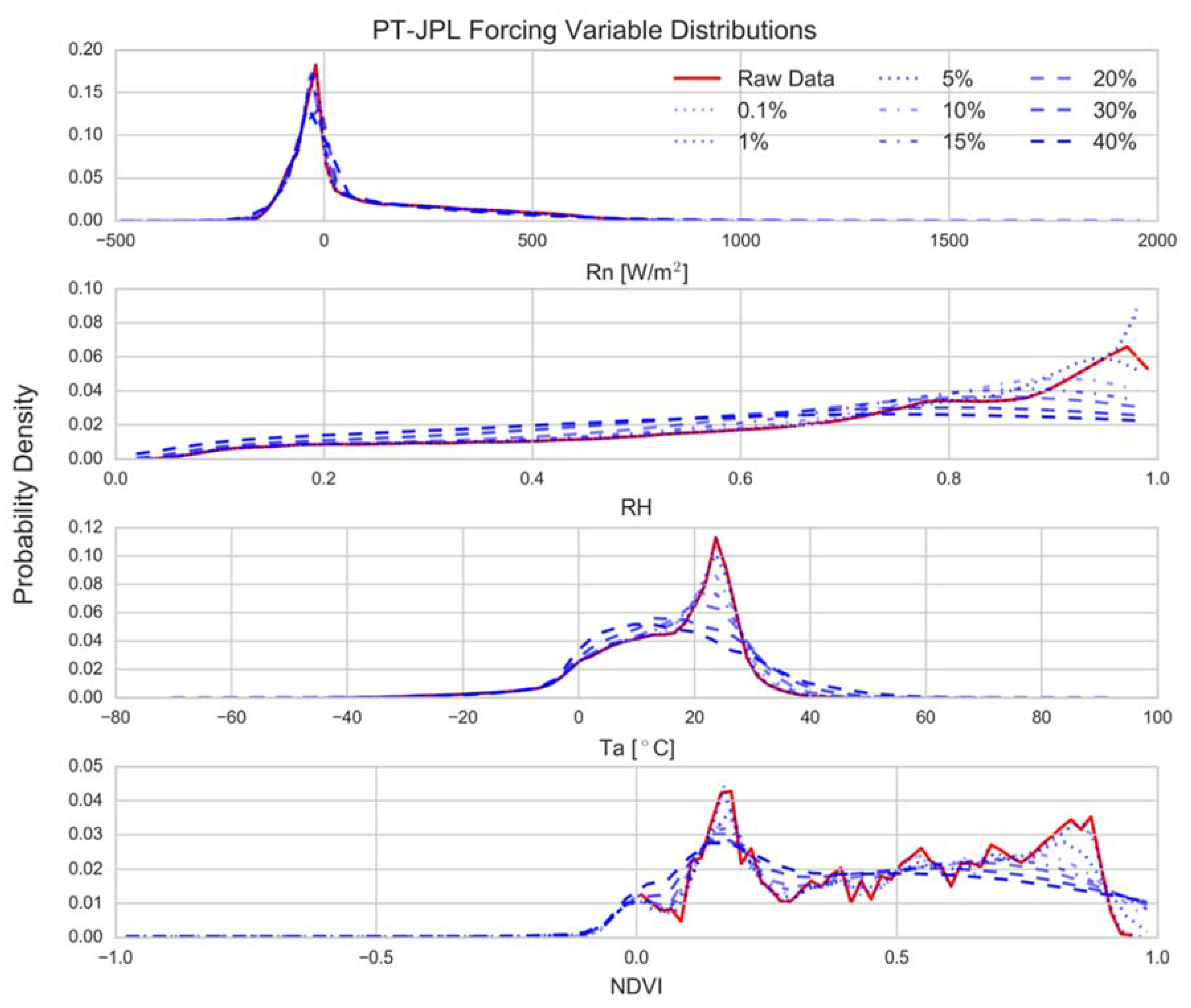
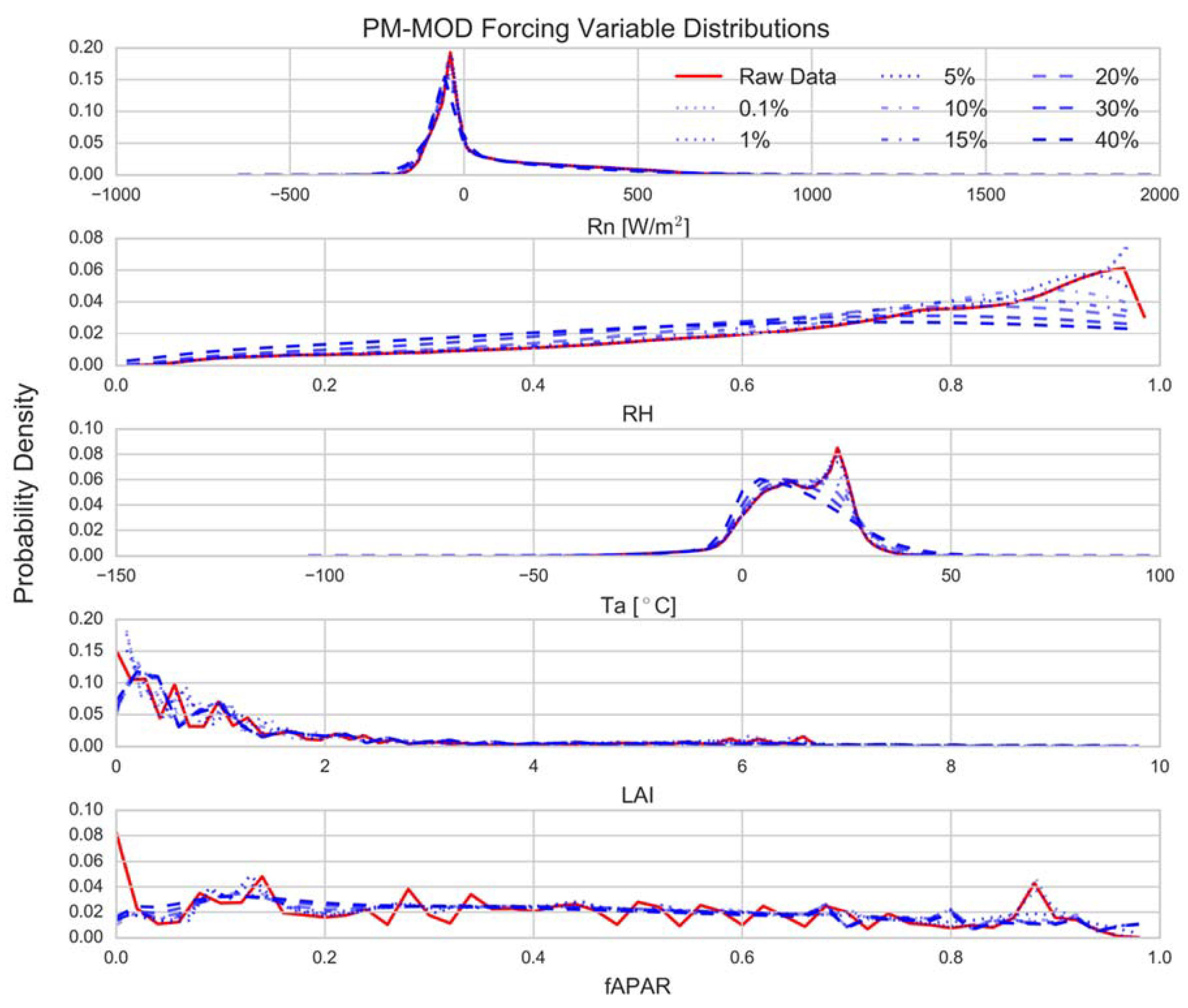
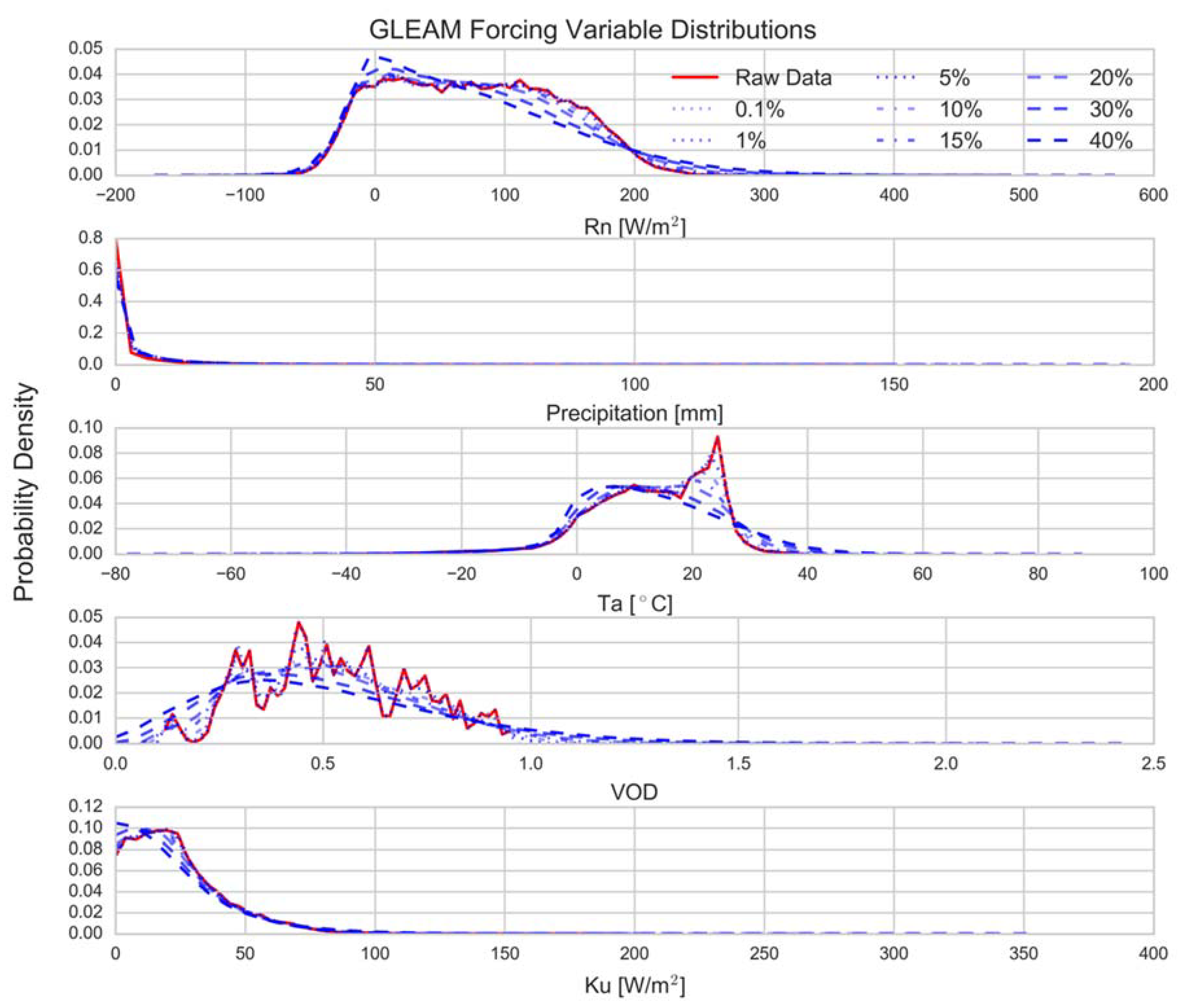
2.2. Monte Carlo Sensitivity Analysis

To assess each model’s relative sensitivity to the forcing, we use a Monte Carlo style simulation [77,78]. This approach involves perturbing each variable by some random uncertainty drawn from a predetermined probability distribution and analysing how the final model output changes in reference to the perturbation. We can then compare the model sensitivity across variables, within variable ranges and across models. As such, the sensitivity of the models to the dynamic forcing (Table 2) is examined. GLEAM, and, to a lesser extent, PM-MOD and PT-JPL use static parameters and variables that vary in space but do not vary in time. While these variables are important to the partitioning within the models, this study does not consider the sensitivity of the models to these constants.

Several of the forcing products in Table 2 are derived from re-analysis products that are the result of model simulations which incorporate observations from balloon soundings, satellite data and in situ measurements in a data assimilation system. Furthermore, the original products have been pre-processed further to create a common spatial and temporal scale. Therefore, data quality will change in time and space [73] and an accurate estimate of the product uncertainty is difficult to determine. To account for potential changes in forcing uncertainty, different Monte Carlo experiments will be performed with different perturbation strengths in order to analyse how the model outputs respond to various uncertainty ranges.

For unbounded forcing we assume a Gaussian error distribution to describe the errors, while we use a truncated-normal distribution to describe the errors of the bounded variables. Bounded variables included relative humidity (RH, 0–1), leaf area index (LAI, 0–∞ m²/m²), normalized difference vegetation index (NDVI, −1.0–1.0), fraction of absorbed photosynthetically active radiation (fAPAR, 0–1), precipitation (P, 0–∞ mm/day), Vegetation Optical Depth (VOD, 0–∞) and shortwave incoming radiation (Ku, 0–∞). Unbounded variables included net radiation (Rn) and temperature (Ta). For each time step, location and variable, we create a theoretical distribution from which we randomly sample. In all cases, the expected mean value comes from the value of raw forcing variable and the standard deviation of the distribution is a predetermined percentage of the raw value at eight stepwise intervals (0.1%, 1%, 5%, 10%, 15%, 20%, 30% and 40%). At an uncertainty level of 40%, many of the variables have collapsed to distributions in which more uncertainty would not significantly change the distribution of forcing data and model components have broken down to unrealistic flux estimates. Furthermore, the boundary effects of bounded variables could skew model sensitivity at large uncertainty.

If we assume that a large number of sources contribute to the uncertainty and noise of a remotely sensed variable, then by the central limit theorem we can approximate the uncertainty of that variable using a Gaussian distribution. The Gaussian distribution allows us to perturb the data while conserving the original unperturbed value as the mean of the distribution. Thus, any bias found in the distribution of the sensitivity results will reflect non-linear formulations within the model. While this distribution may not reflect the reality of the uncertainty contained within the data, it allows us to observe how the model formulation might propagate error in a way that would introduce bias to the final estimates. Thus, we assume that the forcing does not contain any systematic bias in its error.

The truncated-normal distribution is a combination of a mean conserving distribution with a mean changing shift, so that bounded variables may not preserve the original mean [79]. The truncated-normal distribution is advantageous over a beta or gamma distribution because we can specify large uncertainties without the distribution collapsing toward probability masses located only at one or both bounds. If a variable is bounded on one side or if the original mean is closer to one of the bounds, then the expected mean of the resulting distribution will shift away from that bound. The resulting magnitude of the shift is a function of the difference between the bound and the original mean and the level of added uncertainty. The resulting shift is therefore more likely to influence the results found here if the added uncertainty is high or if the original variable is closer to one of the bounds.

Figure 1, Figure 2 and Figure 3 show the probability distribution functions for the entire study period over all sites. The distributions show both the raw unperturbed data and the distribution of data after perturbation at various uncertainty levels. Note that these figures show the distributions of the original and perturbed data and not the theoretical distributions used to generate random error. PT-JPL and PM-MOD show identical distributions for common forcing variables. For forcing variables common to the GLEAM model, such as net radiation or air temperature, the distributions are slightly different due to the difference in temporal resolution.

2.3. Error and Bias Assessment

As previously stated, we forced the three models for three years (2003–2005) at 42 locations where model output has previously been evaluated against field-based estimates of ET components [18]. Random error was added to each forcing variable based on the described probability distributions and each data point was sampled 100 times. This process was repeated at each assumed uncertainty level and for each variable field. In this study, we cannot determine the exact uncertainty for each forcing variable or the correct combination of forcing variable uncertainty. We perturb only one variable at a time, as this allows us to disentangle the effect of the individual forcing variables and evaluate them in isolation.

After the model simulation, we then calculate the relative error for each model and evaporation component (RE):

$$RE=\frac{y_i-y_0}{y_0}$$

(1)

where $y_i$ is the perturbed estimate and $y_0$ is the unperturbed estimate of the ET component. We then pool the relative error at each time, location and random sample and analyse the results as a distribution of the relative error values. We analyse the resulting distribution using two objective functions: percent root mean squared deviation (%RMSD, Equation (2)) and percent mean bias deviation (%MBD, Equation (3)). Both functions are calculated at an added uncertainty (σ) of 10% and are normalized by the mean total ET estimate for the model across all standard outputs (i.e., no added uncertainty) and expressed as a percentage of total ET:

$$\%RMSD=\frac{100}{\overline{ET}}\sqrt{\frac{{\sum }_{i,x}^N{\left({\dot{y}}_{i,x}-y_{i,x}\right)}^2}{N}},$$

(2)

And

$$\%MBD=\frac{100}{\overline{ET}}\left(\frac{{\sum }_{i,x}^N\left({\dot{y}}_{i,x}-y_{i,x}\right)}{N}\right).$$

(3)

where ${\dot{y}}_{i,x}$ represents the estimated value after perturbation, $y_{i,x}$ is the original estimate, N is the total number of estimates, $x$ is the specific location and $i$ the specific time and $\overline{ET}$ is the model-specific mean ET over all locations and time. 10% was chosen because it represents significant added uncertainty while avoiding the boundary effects of larger uncertainties.

3. Results

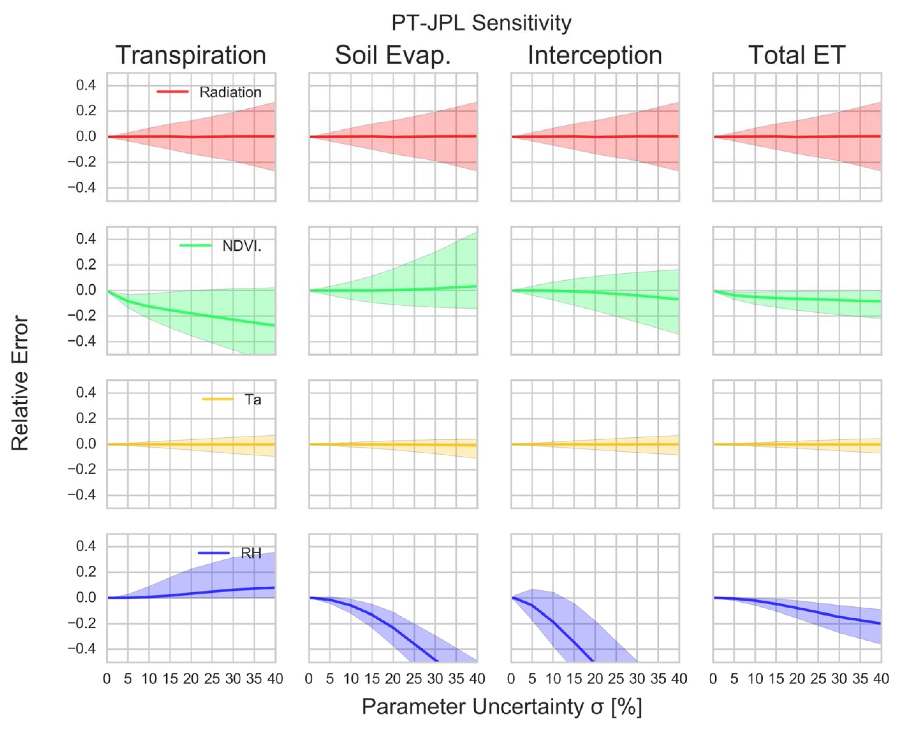
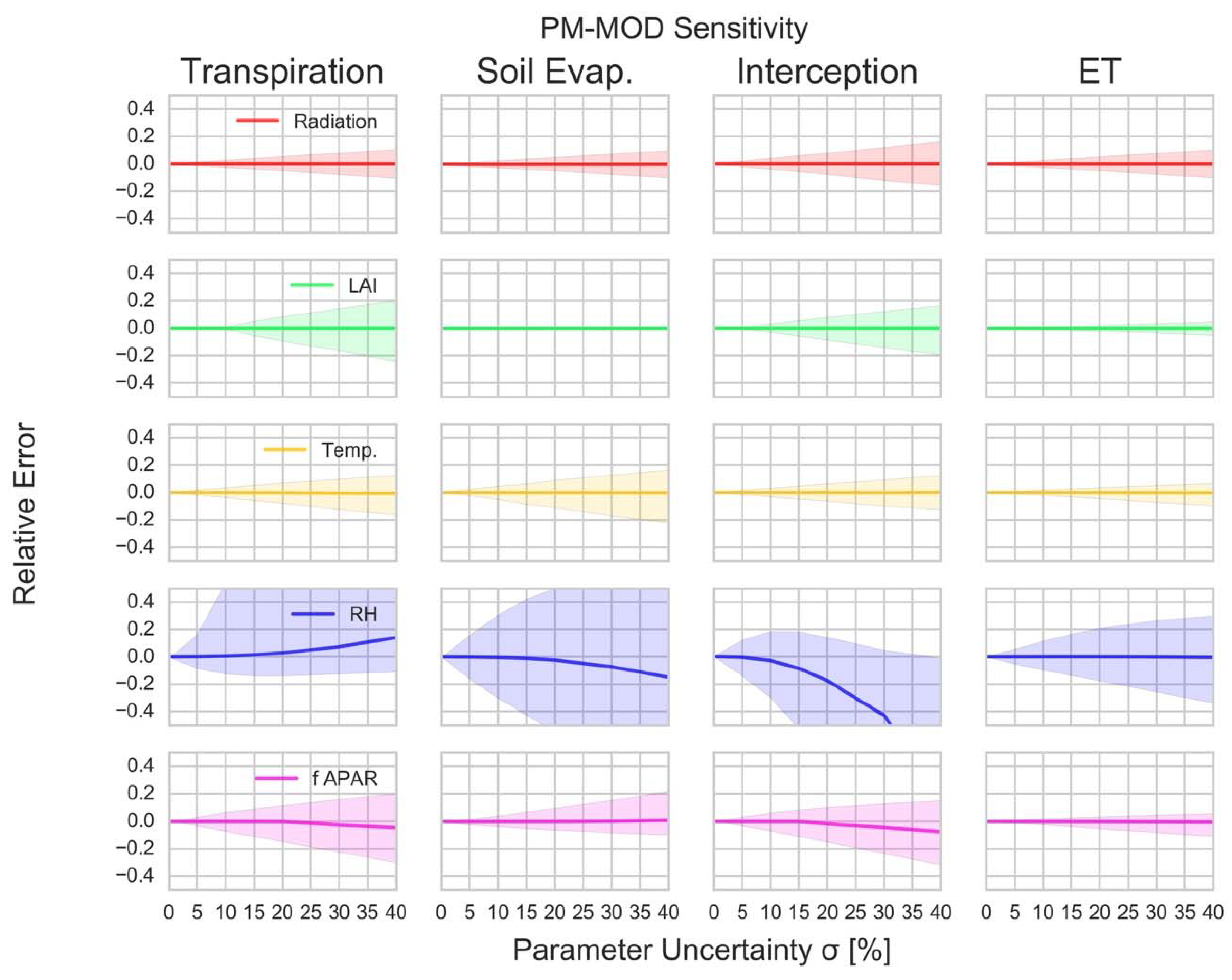
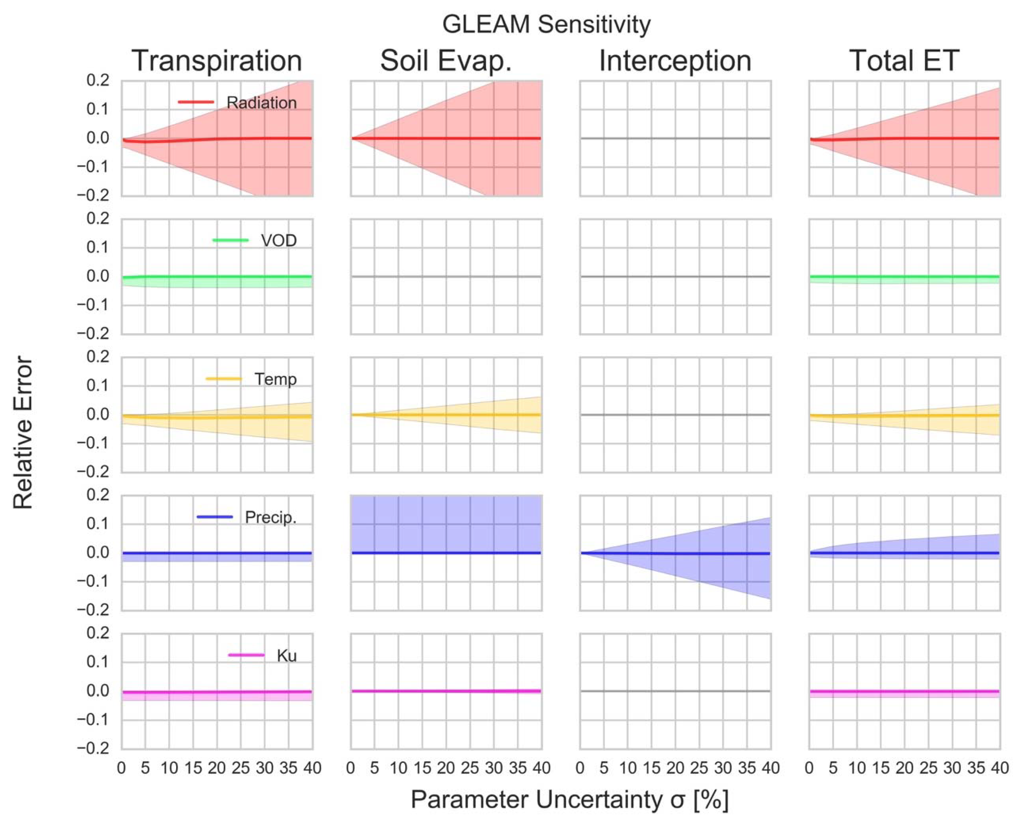
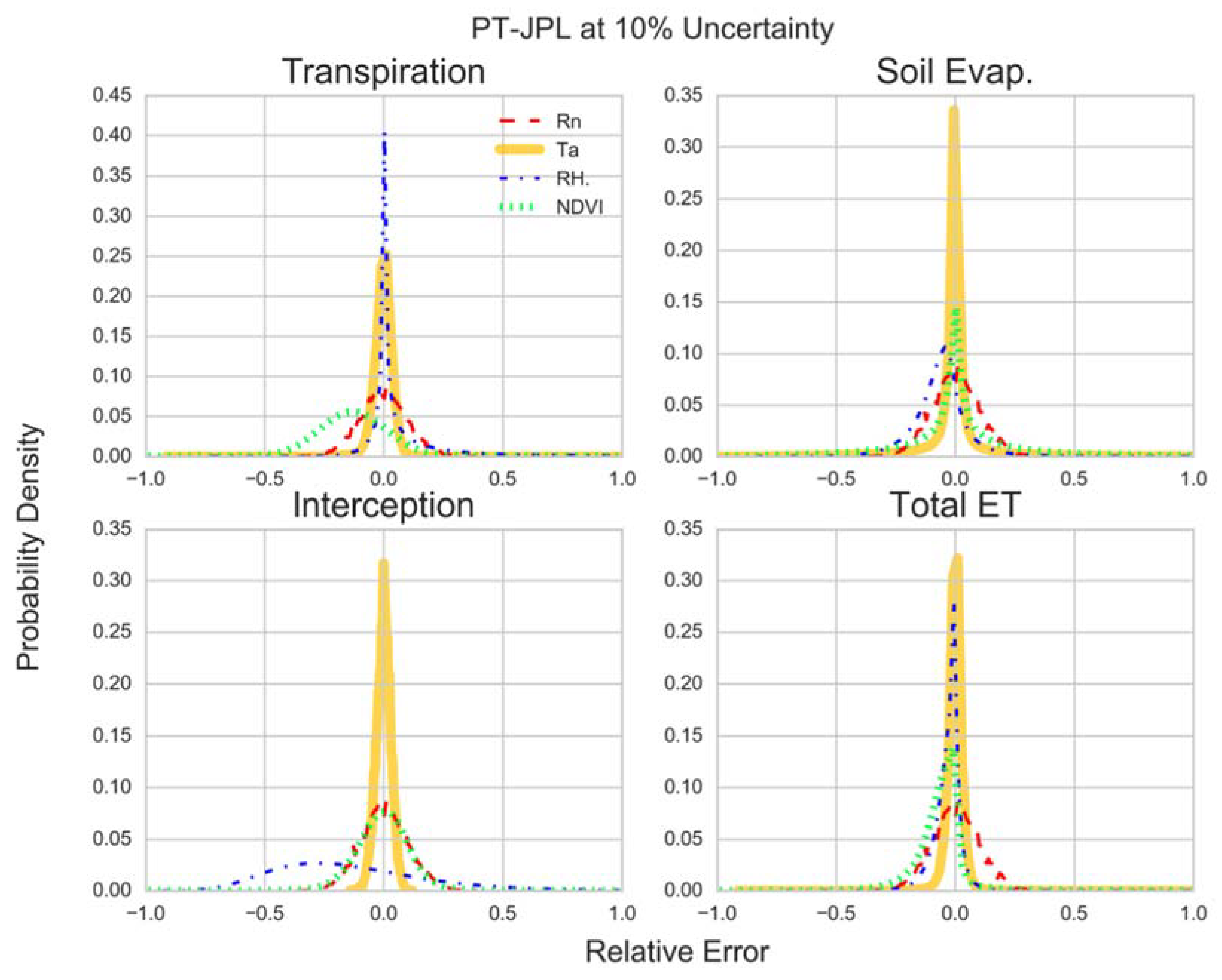
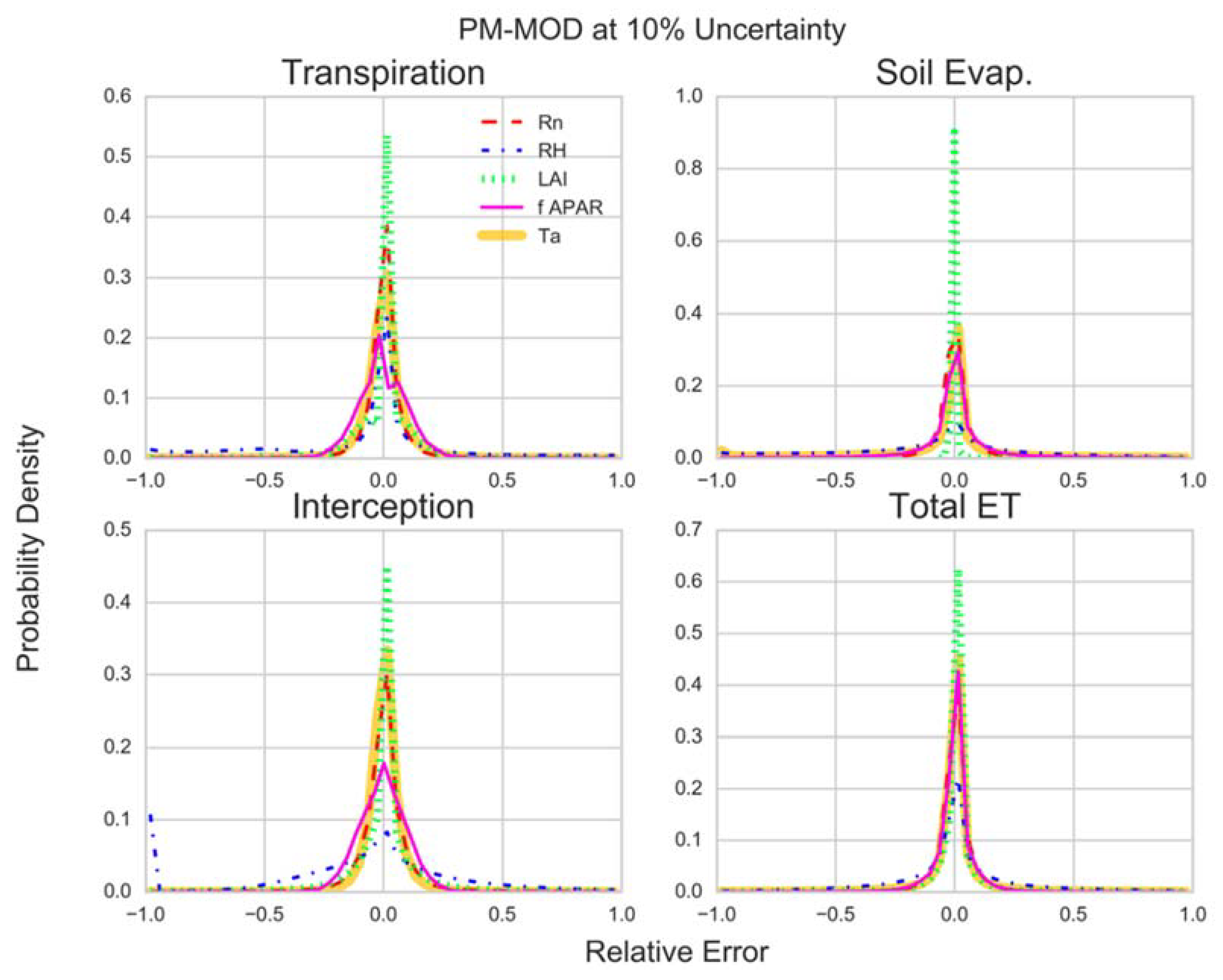
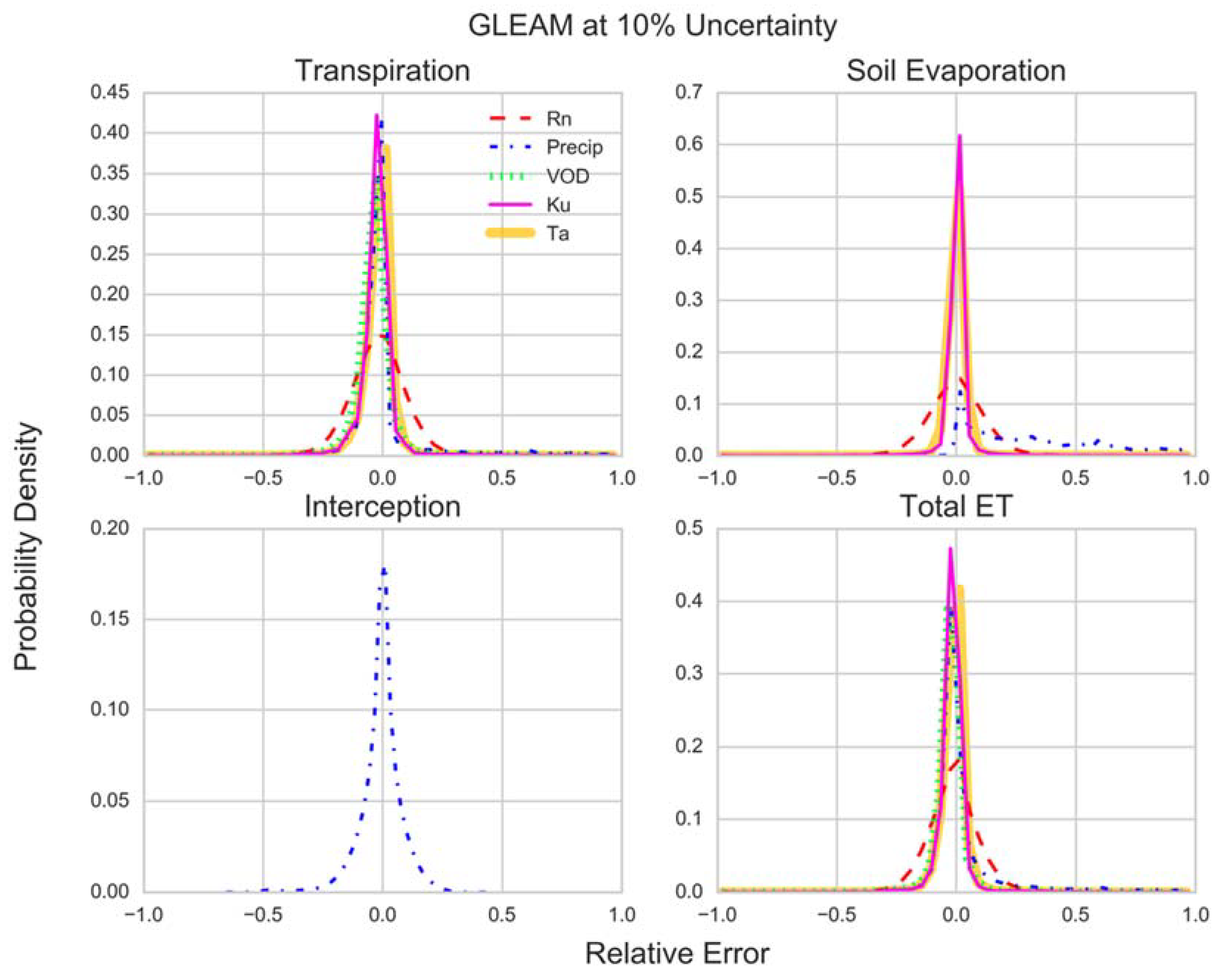
3.1. Model Sensitivity Distributions

Figure 4, Figure 5 and Figure 6 show the sensitivity of the model output to each of the forcing variables for different uncertainty levels. The plots show the interquartile range of the distribution of relative error between perturbed and unperturbed forcing for each uncertainty level, as well as the median of the distribution. Generally, a greater interquartile range signifies that the model is more sensitive to that forcing variable. The deviation of the median from a relative error of 0 signifies asymmetry in the model response to forcing uncertainty due to non-linearity in the model formulation.

While the interquartile range and median give us an idea of the distributions of error at across increasing amounts of uncertainty, they do not represent the entire distribution. Figure 7, Figure 8 and Figure 9 show the probability distributions of the relative error for each forcing variable and each modelled ET component at an added uncertainty of σ = 10%.

Table 3. Percent root mean squared deviation (%RMSD) and percent mean bias deviation (%MBD) of the distribution of deviation in model estimates of transpiration (E_veg), soil evaporation (E_soil), interception (E_int) and total evapotranspiration (ET) due to variable perturbations. Each value is normalized by the mean ET estimate across the raw dataset for that model. NA values represent instances where the forcing variable for a model is not an input of the specific model component.

	PT-JPL
	%RMSD				%MBD
	Eveg	Esoil	Eint	ET	Eveg	Esoil	Eint	ET
Rn	38.8	38.8	38.8	38.8	1.4	1.4	1.4	1.4
RH	122.6	60.6	151.4	33.1	41.9	−26.1	−59.0	−12.9
Ta	32.3	71.3	13.6	35.9	0.9	−2.3	0.5	0.5
NDVI	91.0	112.0	51.4	100.0	−51.4	5.1	−1.4	−20.0
	PM-MOD
	%RMSD				%MBD
	Eveg	Esoil	Eint	ET	Eveg	Esoil	Eint	ET
Rn	47.4	49.6	42.4	49.1	−0.3	−2.3	0.2	−0.5
RH	144.5	174.2	129.3	122.3	−25.3	−33.7	−19.2	−2.7
Ta	48.3	125.7	28.0	68.1	1.0	−18.6	1.3	1.2
fAPAR	44.2	83.3	30.8	44.0	−0.6	−0.8	−0.6	−1.1
LAI	37.7	8.7	45.5	38.6	0.4	−0.4	0.3	0.4
	GLEAM
	%RMSD				%MBD
	Eveg	Esoil	Eint	ET	Eveg	Esoil	Eint	ET
Rn	8.07	8.15	NA	7.49	−1.16	−0.03	NA	−0.83
P	4.54	4.07	4.10	4.82	−0.74	0.80	−0.14	0.02
Ta	4.49	2.79	NA	3.88	−1.14	0.00	NA	−0.80
Ku	3.96	2.69	NA	3.28	−1.13	0.02	NA	−0.78
VOD	3.94	NA	NA	3.21	−1.16	NA	NA	−0.85

shows the root mean squared deviations (%RMSD, Equation (2)) and mean biased deviation (%MBD, Equation (3)) for each of the variables and each modelled ET component at this uncertainty level. The values in Table 3 are expressed as a percentage of the mean ET estimate across all data points.

PT-JPL takes four forcing variables: net radiation, NDVI, temperature and RH. Each of the modelled ET components varies linearly with net radiation. Figure 4 shows that the relative error also increases linearly with increasing uncertainty in the net radiation term as expected due to the linear formulation of radiation within each model. Due to this linear relationship, there is little to no bias in the model output associated with uncertainty in net radiation evidenced by a MBD of 1% for all ET components. Similarly, the sensitivity of the model is unbiased to uncertainties in temperature, yet this sensitivity is much lower. For RH and NDVI, however, the model shows strong bias in relative error due to forcing uncertainty. The transpiration component of PT-JPL shows a strong negative bias (MBD = −51%) due to uncertainty in NDVI, while showing a positive bias (MBD = 42%) due to uncertainty in RH. The soil evaporation and interception components show a strong negative bias (MBD = −26%, −59%, respectively) due to uncertainty in RH. Interestingly, the contrasting biases in the ET components due to uncertainty in the RH term only result in a slight negative bias (MBD = −13%) in the total ET term and a much smaller RMSD (33%) compared to the components RMSD, which typically ranges between 61 and 151%. The asymmetry in PT-JPL’s response to changes in NDVI and RH is clearly shown in Figure 7, as are the relative sensitivities to the input variables. Strong negative bias in the transpiration component due to NDVI and in the soil evaporation component due to RH are evident. Radiation shows a symmetric distribution with moderate sensitivity across all components, while temperature shows a similar symmetry with relatively subdued sensitivity.

PM-MOD has five temporally variable forcings: net radiation, RH, temperature, fAPAR and LAI. Each of the ET components estimated by PM-MOD is exceedingly sensitive to RH and has negative bias associated with RH. Figure 5 shows that as uncertainty increases, the median of the RH and fAPAR terms increases its deviation from 0. The total ET estimate is similarly sensitive to RH (RMSD = 122%), while the bias becomes somewhat mitigated when the components are aggregated (MBD = −3%). Figure 8 shows that large masses of probabilities associated with RH aggregate in the transpiration and interception terms at a relative error of −1, signifying that a change to RH caused the new model estimate to collapse to 0 flux. The soil evaporation estimate appears to be particularly sensitive to changes in the forcing variables, as perturbations to RH (RMSD = 174%), temperature (RMSD = 132%), net radiation (RMSD = 50%) and fAPAR (RMSD = 84%) all exhibit their largest MBD and RMSD in the soil evaporation term.

GLEAM has seven temporally variable forcings: net radiation, temperature, precipitation, vegetation optical depth (VOD), shortwave incoming radiation (Ku), surface soil moisture and snow water equivalent. Only the first five are evaluated here. GLEAM, among the three models, shows the least sensitivity to its forcing, as evidenced by the low RMSD and MBD. Again, the daily resolution of the model likely plays a factor, as daily estimates of ET must be less variable than sub-daily estimates. Each of the variables show a slight negative bias in the transpiration estimate and precipitation shows a negative bias in the total ET estimate. Figure 9 shows a curious distribution of error associated with precipitation in the soil evaporation term with a large positive tail. The interquartile range for several variables looks quite skewed in Figure 6, including VOD, Ku and precipitation in many cases. While the skew appears quite severe, the median remains near zero and the MBD remains quite small. Figure 9 shows that the vast majority of perturbations of VOD, Ku and precipitation result in little to no model response. Precipitation is the only dynamic variable influencing the GLEAM interception estimate while soil evaporation, transpiration and the overall ET estimates appear primarily influenced by net radiation in our set of study sites (RMSD = 8.2, 8.2 and 7.6% respectively).

PM-MOD and PT-JPL share many similarities both in their formulation and in the results found here. Both models show large biases and uncertainty in their components associated with RH. However, in both models these biases do not manifest to the same extent in the total ET estimates. A similar pattern is also evident for both models in their vegetation forcing. Both NDVI in PT-JPL and fAPAR in PM-MOD show large uncertainties with some bias in their component terms, while the total ET term exhibits far less sensitivity. Temperature and radiation also show similar patterns in sensitivity across components, although PT-JPL generally exhibits a lower %RMSD. Both models show an increased sensitivity to temperature in the soil evaporation term and both have similar ranges of RMSD associated with net radiation.

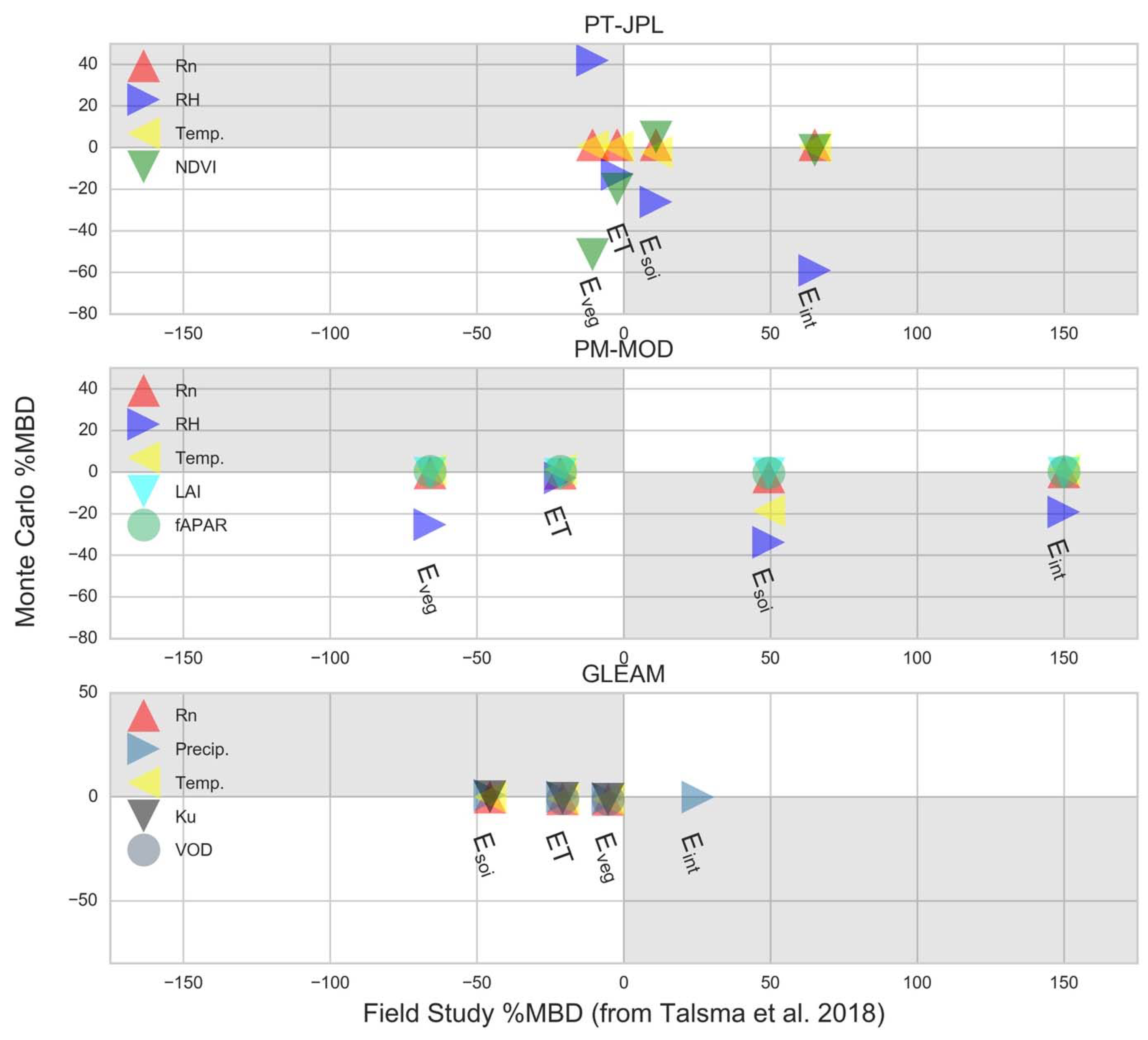
3.2. Model-Field Sensitivity Inter-Comparison

Figure 10 shows the %MBD from the Monte Carlo analysis at an added variable uncertainty of σ = 10% compared with the %MBD between modelled and field estimates of ET components [18]. The forcing data used in both analyses are identical and we can thus directly compare the results of the field comparison study with the Monte Carlo results presented here. The comparison between the two studies allows us to determine if uncertainty in the forcing of each model could be responsible for model deviations from observed field data. While we cannot be certain that the added uncertainty level of each forcing variable is correct, we can determine if the sign (positive/negative) of the %MBD from each analysis is consistent. The field estimates are subject to their own methodological errors and uncertainties and tend to be much smaller in spatial scale compared to the remote sensing estimates. However, we assume that aggregating these studies across many methods and study sites offers valuable information about the partitioning of the ET flux.

The Monte Carlo analysis of PM-MOD shows large negative bias due to the propagation of uncertainty in RH for soil evaporation and interception. However, Figure 10 shows that this negative bias is inconsistent with the positive bias found between the modelled soil evaporation and interception estimates with field estimates. Previous research shows that PM-MOD tends to overestimate these components [18], while added variable uncertainty would result in an underestimation. Thus, uncertainty in RH can be eliminated as the primary driver for the deviation between these modelled ET components and field estimates. The direction of the bias due to RH uncertainty is consistent with field comparisons in the transpiration term. This suggests that forcing uncertainty could indeed be responsible for the observed bias in this term.

Similarly, Figure 10 shows that much of the bias found in PT-JPL due to the propagation of forcing uncertainty is inconsistent with the observed bias between modelled and field-based estimates, particularly for RH. However, bias due to the propagation of added uncertainty in NDVI in transpiration, soil evaporation and total ET are consistent with the field bias. RH also shows consistent bias estimates within the PT-JPL total ET estimate. GLEAM shows very little bias due to the propagation of forcing uncertainty. Thus, forcing uncertainty is likely not responsible for the model deviation with field estimates shown in Figure 10.

3.3. Model Sensitivity across Forcing Conditions

Figure 11, Figure 12 and Figure 13 show the sensitivity of each model to perturbations in the forcing categorized as a function of the forcing (without perturbation) itself. The figures show the interquartile range and median of the relative error associated with an uncertainty of 10%. These figures allow us to analyse how the model sensitivity changes based on the physical conditions at a given location. The figures show trends in both the median and interquartile range values as forcing variables change suggesting that model bias and sensitivity are dependent on ambient conditions.

PT-JPL shows a steady distribution with changing net radiation and temperature, while both the median and interquartile range of the error distribution changes with RH and NDVI. However, the changes to uncertainty in the estimated ET components again counteract each other and, as such, limit the uncertainty in the total ET estimate at each of the ranges in forcing values. Both PM-MOD and PT-JPL exhibit the same increasing uncertainty with increasing RH in their transpiration component and again show similar increasing uncertainty in soil evaporation with increasing vegetation indices. PM-MOD, shown in Figure 13, appears to be more sensitive to changes at extreme temperatures than to changes at more moderate temperatures. Interestingly, PM-MOD soil evaporation appears to be more sensitive to lower LAI values but also more sensitive to higher values of fAPAR. GLEAM, shown in Figure 13, is overwhelmingly more sensitive to changes in low precipitation events than larger events. Net radiation and temperature show relatively unbiased and consistent distributions in error as those variables change, while VOD and Ku show somewhat more asymmetric distributions with an unbiased median.

4. Discussion

The results of this study are able to offer insights into how the uncertainty of temporally variable forcing influences the model estimates. Of particular interest are the differences in how the forcing affects the component estimates as compared to the total ET estimate and how uncertainty in the forcing combined with non-linear model formulations can introduce a bias. Also of interest is how this uncertainty in the forcing might manifest when comparing model estimates against field based data.

4.1. Model Sensitivity

Despite some similarities in model formulation, each model exhibits its greatest sensitivity to a different forcing variable. GLEAM interception is exclusively sensitive to precipitation, while the remainder of the GLEAM components are largely sensitive to net radiation, soil evaporation especially. These results are nonetheless dependent on the study locations adopted and previous studies have shown a larger sensitivity of GLEAM estimates on the precipitation and surface soil moisture (not considered here) forcing data in the case of drier regions [80]. While PT-JPL and PM-MOD are also sensitive to net radiation, they are far more sensitive in each of their component estimates to RH and vegetation forcing. The PT-JPL ET estimate appears to be very sensitive to changes in NDVI (RMSD = 1.01) likely due to the roll of NDVI in parameterizing vegetation characteristics. Similarly, the PM-MOD ET estimate is most sensitive to changes in RH (RMSD = 1.22) largely driven by the soil evaporation term. It should also be stressed that these results are representative of only the study sites used and the global sensitivity of each model could change with a more globally representative set of study sites.

The soil evaporation term of PT-JPL and PM-MOD show very little agreement and large variance when compared with field estimates [18]. Here, we find soil evaporation for those models to be generally quite sensitive to uncertainty in the variables of RH, temperature, NDVI and fAPAR. These errors are distributed across impacts from the partitioning of net radiation between the canopy and soil surface using NDVI or fAPAR and water availability limitations inferred from RH and temperature. Furthermore, the sensitivity of the soil evaporation estimate appears to vary depending on the value of the variable itself. These factors could explain the large variance in their agreement with the field studies. The use of proxies to estimate soil moisture by PM-MOD and PT-JPL likely introduces some uncertainty to the soil evaporation estimate and could explain the outsized role of soil evaporation in the global partitioning of ET for those models [17]. GLEAM uses soil moisture data assimilation to incorporate direct measurements of surface soil moisture. However, the data assimilation is not incorporated in this study.

Given the high sensitivity of soil evaporation to forcing uncertainty in each of the models, this component could be responsible for a large portion of the partitioning divergence between models. Improvement of the soil evaporation term, therefore, offers a potential area in which to focus efforts in order to improve model partitioning. Similarly, a study of North American Land Data Assimilation System (NLDAS) ET models shows that uncertainty in soil evaporation contributes significantly to uncertainty in the partitioning of the ET flux [81]. Those results also demonstrate that the ability of the model to estimate transpiration is largely responsible for its ability to estimate the total flux. Despite the inability to estimate soil evaporation or correctly partition the flux, the total ET estimate remained reasonably accurate. Furthermore, counteracting biases in the ET components from PT-JPL and PM-MOD show a decreased sensitivity of the total ET estimate to forcing as compared to the component estimates.

GLEAM, however, appears to be much more reliant on the underlying formulation of the model and model constants than on its forcing variables. The RMSD and MBD exhibited by GLEAM is roughly an order of magnitude smaller than that of PM-MOD and PT-JPL. Given the higher complexity of GLEAM compared to the other two models, it might be expected that GLEAM would be more sensitive to model formulations and constants, more constrained with respect to any single variable and rather robust to changes in forcing uncertainty. The daily resolution of GLEAM also means that estimates are likely less variable than sub-daily estimates and thus less sensitive to changes in forcing. This complexity also makes interpreting the biases of the error distributions in the model more difficult. Precipitation, Ku and VOD exhibit very asymmetric distributions in both Figure 6 and Figure 9. GLEAM shows very few truly linear relationships, as the model relies on water balances, storage capacities and stress factors to account for the water available to various evaporative pathways. Here it results in somewhat skewed distributions in estimates but the various parameterizations within the model can likely be adjusted to accommodate those errors. The distribution of precipitation is also characterized by a large frequency of very small events, which may be prone to biases introduced by the truncated-normal distribution. When perturbed by an increasing level of uncertainty, the distribution collapses so that these small events become less frequent. Given the greater sensitivity to these smaller events shown in Figure 13, the distribution of error then becomes skewed for the various components.

Furthermore, models may be more sensitive to forcing errors at various extremes of that variable. The GLEAM model’s sensitivity to low precipitation events opposed to larger events is due to the fact that large precipitation events wet the soil over the threshold in which evaporation becomes fully energy-driven. The results also show that perturbing precipitation shifts the partitioning of GLEAM from transpiration to soil evaporation at our study sites. Both PM-MOD and PT-JPL transpiration components are more sensitive at high RH values than at lower values. This is due to the fwet term, which exhibits a much higher slope as a function of humidity at high RH values and due to the negative bias introduced by the truncated-normal distribution. PM-MOD ET also shows increasing uncertainty at increasing values of both LAI and fAPAR. In case of fAPAR, the relationship appears to be driven by the soil evaporation term, which is substantially more uncertain at high fAPAR values. PT-JPL exhibits a similar trend in soil evaporation but in the NDVI term.

Where trends exist in the uncertainty of the model with changing ambient conditions informs where these model estimates may be vulnerable to large uncertainties. The partitioning of both PM-MOD and PT-JPL seems particularly sensitive to extremes in vegetation and RH forcing, although RH could be influenced by the distributions used in this analysis. Again, the trends in component uncertainty tend to mitigate one another when aggregated in the total ET estimate of PT-JPL. However, PM-MOD exhibits larger uncertainty in its total ET estimate at elevated values of radiation, vegetation indices and temperature. This is somewhat worrisome considering that the largest fluxes coincide with large values of these variables and represent areas where inaccurate estimates of ET would likely impair global estimates.

4.2. Non-Linearity and Model Bias

The %MBD due to uncertainty in RH in both PT-JPL and PM-MOD is expected due to the non-linear dependence of the ET components to RH within these models. In both models, the model parameter fwet—calculated as a function of RH raised to the forth power—is used to approximate surface wetness. It is important to consider that the relationship between humidity and a given ET component is very likely to be non-linear, making non-linear formulations, as in PT-JPL and PM-MOD, appropriate [28,82]. However, large forcing uncertainties in non-linear models can introduce large biases to the model estimate and thus might debilitate the usefulness of the model. Figure 4 shows how increasing uncertainty in the RH introduces growing bias in the component estimates of PT-JPL and PM-MOD. The point at which this bias becomes detrimental is determined by the uncertainty of the forcing variable. It should be noted that bias could also be introduced to RH by the use of the truncated-normal distribution, although only near the upper bound (Figure 11 and Figure 12). The effects of the truncated-normal on RH are thus difficult to disentangle, as we expect both large bias due to the non-linear formulation and bias due to the effect of the truncated-normal distribution.

Despite the similar use of RH in PT-JPL and PM-MOD, both models do have different error distributions. PM-MOD filters RH values less than 0.7 and masks them with a value of 0, while PT-JPL does not. This filter is likely responsible for the large probability mass in the interception component shown in Figure 8 at a relative error of −1 where added uncertainty has RH values greater than 0.7 to become filtered. Both models are also dependent on vapour pressure deficit (VPD), a function of RH and temperature. PM-MOD is dependent on VPD as part of the Penman-Monteith equation and both models incorporate VPD as part of their soil evaporation estimates. Notice that both PT-JPL and PM-MOD soil evaporation estimates are very sensitive to both RH and temperature and PM-MOD is generally more sensitive than PT-JPL to both RH and temperature, likely due to the employment of VPD.

Interestingly, in many of the instances where bias is exhibited in the modelled components due to the propagation of forcing uncertainty, the biases counteract each other in the aggregate total ET estimate. This is especially true for the terms used to partition the available water or radiation between ET components (RH, NDVI, fAPAR). This could help to explain some of the divergences in partitioning between models as well as the negative bias previously found in the PT-JPL and PM-MOD transpiration estimates when compared to field estimates of transpiration [18]. The negative bias related to NDVI in the PM-MOD transpiration component could also help to explain the relatively small contribution that transpiration makes in the global ET partitioning of PM-MOD [17]. This also implies that uncertainty in the estimated ET components is likely larger than in the total ET estimates. Our results suggest that, for PT-JPL and PM-MOD, slight changes in forcing variables have the potential to vastly change the partitioning of ET while resulting in only modest changes to the overall ET estimate.

4.3. Model-Field Sensitivity Inter-Comparison

While large bias due to variable uncertainty is found in the components of both PM-MOD and PT-JPL, the direction of these biases is often inconsistent with comparisons between modelled and field estimates as shown in Figure 10. Where these biases are inconsistent, we can conclude that forcing uncertainty for that particular variable is not responsible for the deviation with field estimates. However, bias in PT-JPL soil evaporation and transpiration due to uncertainty in NDVI does show error consistent with field comparisons. This suggests that the uncertainty in NDVI may be responsible in contributing significant error to the partitioning of ET within PT-JPL. Given that this study is statistical and we assume the level of added uncertainty, only the direction of the bias and not the magnitude of the bias is important in interpreting Figure 10. Different combinations of forcing uncertainty could potentially lead to results similar to those found in Talsma et al., 2018 [18] and Figure 10 should be used only to identify where variables uncertainty may or may not be contributing to observed deviations. The field estimate themselves also contain errors in their methodology but very few techniques exist to directly measure ET components and the field data represents the best available means to validate the remote sensing-based component estimates.

The strengths of this study lie in its exploration of the sensitivity of the model components apart from total ET, as very few studies have focused on the sensitivity of transpiration, soil evaporation and interception within these models. The study is also able to use a theoretical Monte Carlo framework to show how the combination of forcing uncertainty and non-linear model formulation may introduce bias into the model estimate. We can then assess how this statistical approach may be reflected in the practical use of the models by comparing the Monte Carlo results against the results of Talsma et al. (2018) [18] and the global partitioning of the models in Miralles et al. (2016) [17]. While the study is able to explore the role of forcing uncertainty and sensitivity in these models, we are still unable to identify the definitive source of deviation with the field data. The study also relies on several assumptions about the distribution and magnitude of the forcing uncertainty. It is therefore important to focus on how this theoretical distribution of uncertainty is distorted through its propagation and the sensitivity of the variables relative to each other.

5. Conclusions

The demand for research and data concerning ET and ET components will continue to fuel efforts into various remote sensing-based models [2,23]. However, changes in climate and its related feedbacks will require models to show correct sensitivity to many variables [9,20]. Furthermore, the rapid expansion in remote sensing products, data and techniques [24,83,84] presents challenges in understanding and quantifying how errors and uncertainty within the forcing data will propagate to model estimates [26,27]. The sensitivity analysis in this study allows us to determine what variables drive the individual component estimates and helps to explain why the models achieve accurate ET while employing vastly different ET partitioning strategies. The results of the study present a means to assess the strategies of each model and to compare those strategies against our theoretical understanding of ET and its components. A key finding of this study is the elevated bias found in the component estimates of PM-MOD and PT-JPL related to RH (MBD = −59–41.9%) and NDVI (MBD = −51.4–5.1%) and how these biases are largely balanced when aggregated in the total ET estimate. We are also able to determine if these biases are consistent with model deviations from field estimates (RH for PM-MOD components, PT-JPL interception, PT-JPL soil evaporation) or inconsistent (NDVI for PM-MOD components and ET; RH for PT-JPL transpiration).

The main findings of this study are:

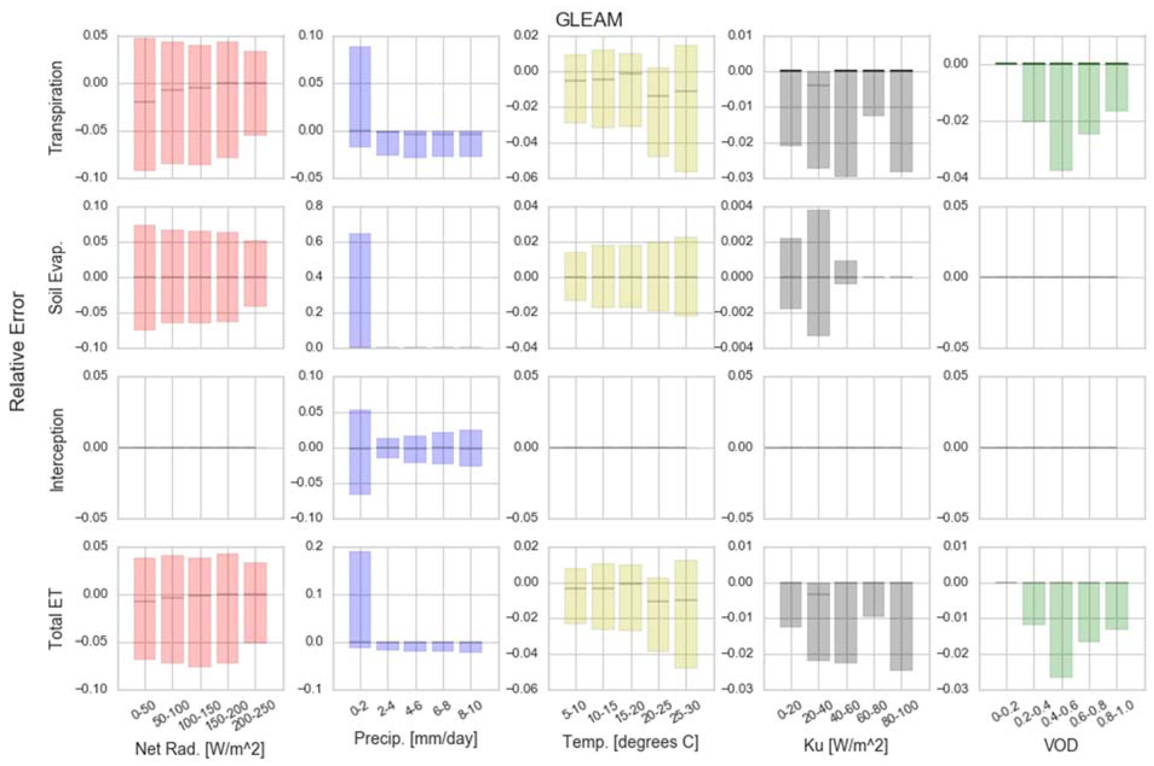
• GLEAM is primarily sensitive to net radiation (RMSD = 7.49–8.07%), except for the interception component, which is driven by precipitation (RMDS = 4.1%).
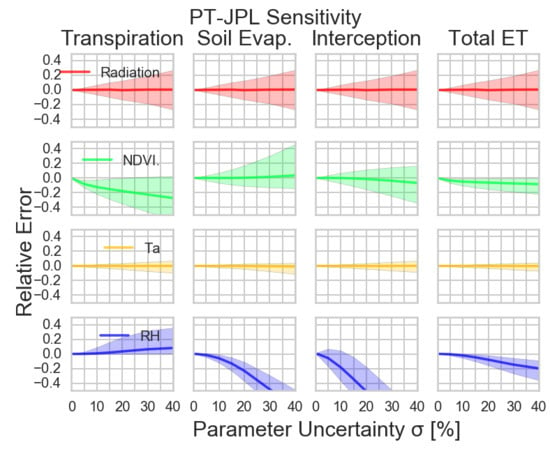
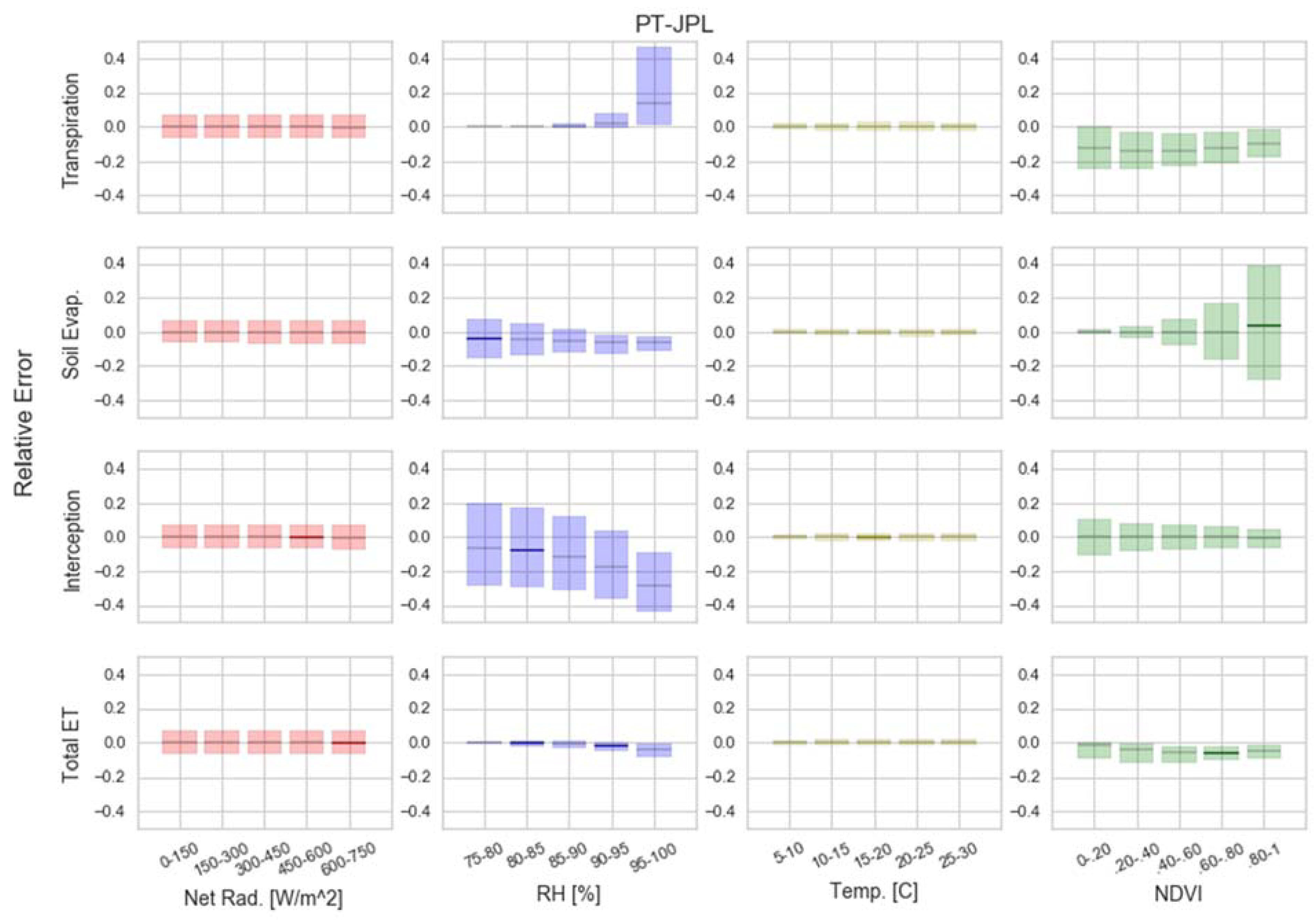
• PT-JPL components are generally sensitive to RH (RMSD = 60.6–151.4%) and NDVI (RMSD = 51.4–112%), while the total ET estimate is most sensitive to NDVI (RMSD = 100%).
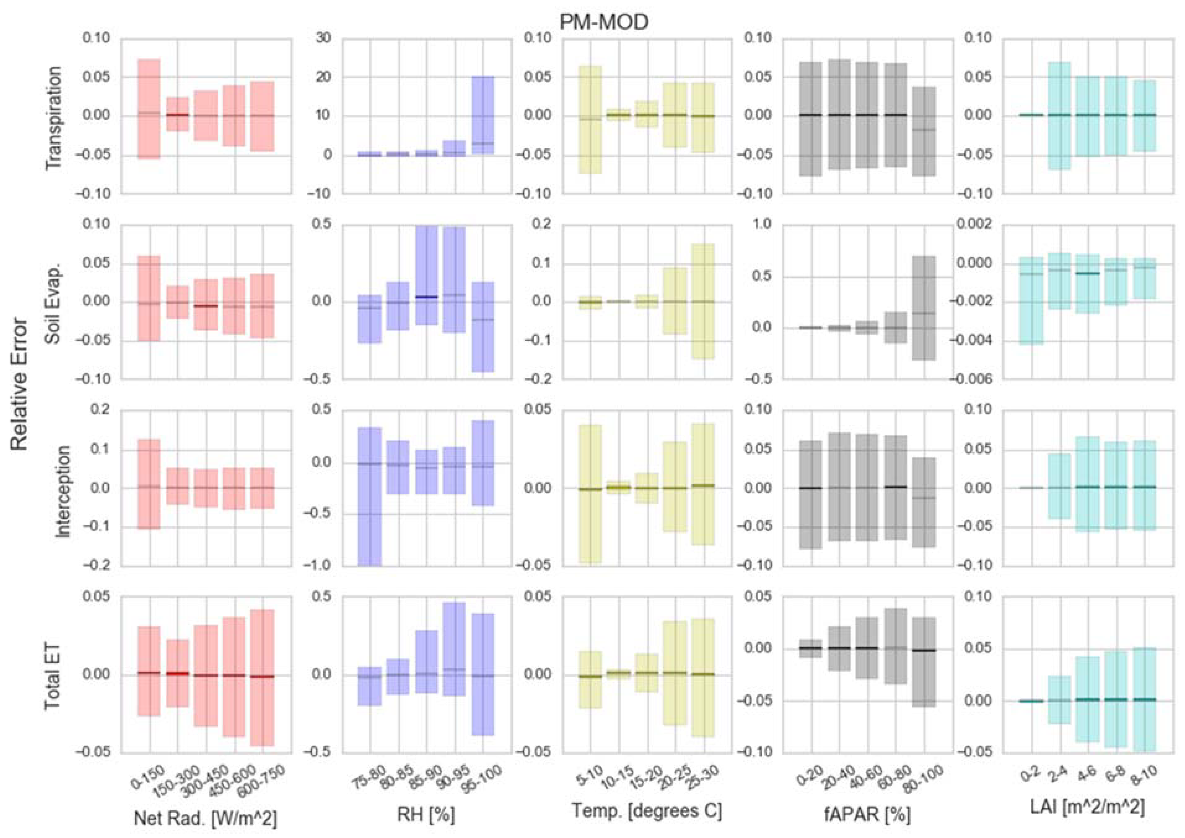
• Both the components and the total ET estimate of PM-MOD are primarily sensitive to RH (RMSD = 122.3–174.2%).
• GLEAM is comparatively less sensitive to changes in its forcing variables than PM-MOD and PT-JPL. The higher complexity and daily resolution of GLEAM makes it more constrained but potentially more sensitive to the model parameterizations. Note that the soil moisture data assimilation of GLEAM was not evaluated here.
• Both PT-JPL and PM-MOD soil evaporation show large sensitivity to forcing inputs, creating greater overall uncertainty in the soil evaporation estimate for our study sites.
• Non-linear formulations of RH and vegetation indices in PT-JPL and PM-MOD often result in large biases (|MBD| > 50%) in component estimates due to variable uncertainty. However, bias in the component estimates often balance each other and limit the bias and uncertainty of the total ET estimate (|MBD| ≤ 20%). Changes to forcing could cause large changes to model partitioning with comparatively smaller changes to the overall ET estimate.
• Bias in PT-JPL due to uncertainties in NDVI are consistent with errors found when comparing model estimates to field estimates. This suggests that uncertainty in NDVI may be introducing significant error to the partitioning of PT-JPL.

References

1. Oki, T.; Kanae, S. Global hydrological cycles and world water resources. Science 2006, 313, 1068–1072. [Google Scholar] [CrossRef] [PubMed]
2. Fisher, J.B.; Melton, F.; Middleton, E.; Hain, C.; Anderson, M.; Allen, R.; McCabe, M.F.; Hook, S.; Baldocchi, D.; Townsend, P.A.; et al. The future of evapotranspiration: Global requirements for ecosystem functioning, carbon and climate feedbacks, agricultural management, and water resources. Water Resour. Res. 2017, 53, 2618–2626. [Google Scholar] [CrossRef] [Green Version]
3. Huntington, T.G. Evidence for intensification of the global water cycle: Review and synthesis. J. Hydrol. 2006, 319, 83–95. [Google Scholar] [CrossRef]
4. Zhang, Y.; Peña-Arancibia, J.L.; McVicar, T.R.; Chiew, F.H.S.; Vaze, J.; Liu, C.; Lu, X.; Zheng, H.; Wang, Y.; Liu, Y.Y.; et al. Multi-decadal trends in global terrestrial evapotranspiration and its components. Sci. Rep. 2016, 6, 19124. [Google Scholar] [CrossRef] [PubMed] [Green Version]
5. Zaitchik, B.F.; Santanello, J.A.; Kumar, S.V.; Peters-Lidard, C.D.; Zaitchik, B.F.; Santanello, J.A.; Kumar, S.V.; Peters-Lidard, C.D. Representation of Soil Moisture Feedbacks during Drought in NASA Unified WRF (NU-WRF). J. Hydrometeorol. 2013, 14, 360–367. [Google Scholar] [CrossRef]
6. Allen, C.D.; Macalady, A.K.; Chenchouni, H.; Bachelet, D.; McDowell, N.; Vennetier, M.; Kitzberger, T.; Rigling, A.; Breshears, D.D.; Hogg, E.H.; et al. A global overview of drought and heat-induced tree mortality reveals emerging climate change risks for forests. For. Ecol. Manag. 2010, 259, 660–684. [Google Scholar] [CrossRef]
7. Spinoni, J.; Naumann, G.; Carrao, H.; Barbosa, P.; Vogt, J. World drought frequency, duration, and severity for 1951–2010. Int. J. Climatol. 2014, 34, 2792–2804. [Google Scholar] [CrossRef]
8. Miralles, D.G.; Gentine, P.; Seneviratne, S.I.; Teuling, A.J. Land-atmospheric feedbacks during droughts and heatwaves: State of the science and current challenges. Ann. N. Y. Acad. Sci. 2018. [Google Scholar] [CrossRef] [PubMed]
9. Friedlingstein, P.; Meinshausen, M.; Arora, V.K.; Jones, C.D.; Anav, A.; Liddicoat, S.K.; Knutti, R.; Friedlingstein, P.; Meinshausen, M.; Arora, V.K.; et al. Uncertainties in CMIP5 Climate Projections due to Carbon Cycle Feedbacks. J. Clim. 2014, 27, 511–526. [Google Scholar] [CrossRef] [Green Version]
10. Mancosu, N.; Snyder, R.; Kyriakakis, G.; Spano, D. Water Scarcity and Future Challenges for Food Production. Water 2015, 7, 975–992. [Google Scholar] [CrossRef] [Green Version]
11. Ciais, P.; Reichstein, M.; Viovy, N.; Granier, A.; Ogée, J.; Allard, V.; Aubinet, M.; Buchmann, N.; Bernhofer, C.; Carrara, A.; et al. Europe-wide reduction in primary productivity caused by the heat and drought in 2003. Nature 2005, 437, 529–533. [Google Scholar] [CrossRef] [PubMed]
12. Meng, X.H.; Evans, J.P.; McCabe, M.F.; Meng, X.H.; Evans, J.P.; McCabe, M.F. The Impact of Observed Vegetation Changes on Land–Atmosphere Feedbacks During Drought. J. Hydrometeorol. 2014, 15, 759–776. [Google Scholar] [CrossRef] [Green Version]
13. Goulden, M.L.; Bales, R.C. Mountain runoff vulnerability to increased evapotranspiration with vegetation expansion. Proc. Natl. Acad. Sci. USA 2014, 111, 14071–14075. [Google Scholar] [CrossRef] [PubMed] [Green Version]
14. Porkka, M.; Gerten, D.; Schaphoff, S.; Siebert, S.; Kummu, M. Causes and trends of water scarcity in food production. Environ. Res. Lett. 2016, 11, 015001. [Google Scholar] [CrossRef] [Green Version]
15. Dolman, A.J.; Miralles, D.G.; de Jeu, R.A.M. Fifty years since Monteith’s 1965 seminal paper: The emergence of global ecohydrology. Ecohydrology 2014, 7, 897–902. [Google Scholar] [CrossRef]
16. McCabe, M.F.; Rodell, M.; Alsdorf, D.E.; Miralles, D.G.; Uijlenhoet, R.; Wagner, W.; Lucieer, A.; Houborg, R.; Verhoest, N.E.C.; Franz, T.E.; et al. The future of Earth observation in hydrology. Earth Syst. Sci. 2017, 21, 3879–3914. [Google Scholar] [CrossRef] [PubMed] [Green Version]
17. Miralles, D.G.; Jiménez, C.; Jung, M.; Michel, D.; Ershadi, A.; McCabe, M.F.; Hirschi, M.; Martens, B.; Dolman, A.J.; Fisher, J.B.; et al. The WACMOS-ET project-Part 2: Evaluation of global terrestrial evaporation data sets. Hydrol. Earth Syst. Sci. Discuss. 2016, 12, 10651–10700. [Google Scholar] [CrossRef]
18. Talsma, C.J.; Good, S.P.; Jimenez, C.; Martens, B.; Fisher, J.B.; Miralles, D.G.; McCabe, M.F.; Purdy, A.J. Partitioning of evapotranspiration in remote sensing-based models. Agric. For. Meteorol. 2018, 260, 131–143. [Google Scholar] [CrossRef]
19. Bonan, G.B. Forests and climate change: Forcings, feedbacks, and the climate benefits of forests. Science 2008, 320, 1444–1449. [Google Scholar] [CrossRef] [PubMed]
20. Lawrence, D.M.; Thornton, P.E.; Oleson, K.W.; Bonan, G.B.; Lawrence, D.M.; Thornton, P.E.; Oleson, K.W.; Bonan, G.B. The Partitioning of Evapotranspiration into Transpiration, Soil Evaporation, and Canopy Evaporation in a GCM: Impacts on Land–Atmosphere Interaction. J. Hydrometeorol. 2007, 8, 862–880. [Google Scholar] [CrossRef]
21. Wang, L.; Good, S.P.; Caylor, K.K. Global synthesis of vegetation control on evapotranspiration partitioning. Geophys. Res. Lett. 2014, 41, 6753–6757. [Google Scholar] [CrossRef] [Green Version]
22. Good, S.P.; Moore, G.W.; Miralles, D.G. A mesic maximum in biological water use demarcates biome sensitivity to aridity shifts. Nat. Ecol. Evol. 2017, 1, 1883–1888. [Google Scholar] [CrossRef] [PubMed]
23. Zhang, Y.; Chiew, F.H.S.; Peña-Arancibia, J.; Sun, F.; Li, H.; Leuning, R. Global variation of transpiration and soil evaporation and the role of their major climate drivers. J. Geophys. Res. Atmos. 2017, 122, 6868–6881. [Google Scholar] [CrossRef]
24. McCabe, M.F.; Aragon, B.; Houborg, R.; Mascaro, J. CubeSats in Hydrology: Ultrahigh-Resolution Insights Into Vegetation Dynamics and Terrestrial Evaporation. Water Resour. Res. 2017, 53, 10017–10024. [Google Scholar] [CrossRef]
25. Michel, D.; Jiménez, C.; Miralles, D.G.; Jung, M.; Hirschi, M.; Ershadi, A.; Martens, B.; McCabe, M.F.; Fisher, J.B.; Mu, Q.; et al. The WACMOS-ET project-Part 1: Tower-scale evaluation of four remote-sensing-based evapotranspiration algorithms. Hydrol. Earth Syst. Sci. 2016, 20, 803–822. [Google Scholar] [CrossRef] [Green Version]
26. Badgley, G.; Fisher, J.B.; Jiménez, C.; Tu, K.P.; Vinukollu, R.; Badgley, G.; Fisher, J.B.; Jiménez, C.; Tu, K.P.; Vinukollu, R. On Uncertainty in Global Terrestrial Evapotranspiration Estimates from Choice of Input Forcing Datasets. J. Hydrometeorol. 2015, 16, 1449–1455. [Google Scholar] [CrossRef]
27. Vinukollu, R.K.; Meynadier, R.; Sheffield, J.; Wood, E.F. Multi-model, multi-sensor estimates of global evapotranspiration: Climatology, uncertainties and trends. Hydrol. Process. 2011, 25, 3993–4010. [Google Scholar] [CrossRef]
28. Fisher, J.B.; Tu, K.P.; Baldocchi, D.D. Global estimates of the land–atmosphere water flux based on monthly AVHRR and ISLSCP-II data, validated at 16 FLUXNET sites. Remote Sens. Environ. 2008, 112, 901–919. [Google Scholar] [CrossRef]
29. Mu, Q.; Zhao, M.; Running, S.W. Improvements to a MODIS global terrestrial evapotranspiration algorithm. Remote Sens. Environ. 2011, 115, 1781–1800. [Google Scholar] [CrossRef]
30. Martens, B.; Miralles, D.G.; Lievens, H.; van der Schalie, R.; de Jeu, R.A.M.; Fernández-Prieto, D.; Beck, H.E.; Dorigo, W.A.; Verhoest, N.E.C. GLEAM v3: Satellite-based land evaporation and root-zone soil moisture. Geosci. Model Dev. 2017, 10, 1903–1925. [Google Scholar] [CrossRef]
31. Miralles, D.G.; Holmes, T.R.H.; De Jeu, R.A.M.; Gash, J.H.; Meesters, A.G.C.A.; Dolman, A.J. Global land-surface evaporation estimated from satellite-based observations. Hydrol. Earth Syst. Sci. 2011, 15, 453–469. [Google Scholar] [CrossRef] [Green Version]
32. Ershadi, A.; McCabe, M.F.; Evans, J.P.; Wood, E.F. Impact of model structure and parameterization on Penman-Monteith type evaporation models. J. Hydrol. 2015, 525, 521–535. [Google Scholar] [CrossRef]
33. McCabe, M.F.; Ershadi, A.; Jimenez, C.; Miralles, D.G.; Michel, D.; Wood, E.F. The GEWEX LandFlux project: Evaluation of model evaporation using tower-based and globally gridded forcing data. Geosci. Model Dev. 2016, 9, 283–305. [Google Scholar] [CrossRef] [Green Version]
34. Priestley, C.H.B.; Taylor, R.J. On the assessment of sruface heat flux and evaporation using large scale parameters. Mon. Weather Rev. 1972, 100, 81–92. [Google Scholar] [CrossRef]
35. Myneni, R.; Knyazikhin, Y.; Park, T. MOD15A2H MODIS/Terra Leaf Area Index/FPAR 8-Day L4 Global 500 m SIN Grid V006. Available online: https://lpdaac. usgs. gov/dataset_discovery/modis/modis_products_table/mod15a2h_v006 (accessed on 16 October 2016).
36. Friedl, M.A.; Sulla-Menashe, D.; Tan, B.; Schneider, A.; Ramankutty, N.; Sibley, A.; Huang, X. MODIS Collection 5 global land cover: Algorithm refinements and characterization of new datasets. Remote Sens. Environ. 2009, 114, 168–182. [Google Scholar] [CrossRef]
37. Poole, D.K.; Roberts, S.W.; Miller, P.C. Water utilization. In Resources Use by Chaparral and Matorral; Miller, P.C., Ed.; Springer: New York, NY, USA, 1981; pp. 123–149. [Google Scholar]
38. McJannet, D.; Fitch, P.; Disher, M.; Wallace, J. Measurements of transpiration in four tropical rainforest types of north Queensland, Australia. Hydrol. Process. 2007, 21, 3549–3564. [Google Scholar] [CrossRef]
39. Calder, I.R.; Wright, I.R.; Murdiyarso, D. A study of evaporation from tropical rain forest—West Java. J. Hydrol. 1986, 89, 13–31. [Google Scholar] [CrossRef]
40. Nizinski, J.J.; Galat, G.; Galat-Luong, A. Water balance and sustainability of eucalyptus plantations in the Kouilou basin (Congo-Brazzaville). Russ. J. Ecol. 2011, 42, 305–314. [Google Scholar] [CrossRef]
41. Leopoldo, P.R.; Franken, W.K.; Villa Nova, N.A. Real evapotranspiration and transpiration through a tropical rain forest in central Amazonia as estimated by the water balance method. For. Ecol. Manag. 1995, 73, 185–195. [Google Scholar] [CrossRef]
42. Salati, E.; Vose, P.B. Amazon Basin: A system in equilibrium. Science 1984, 225, 129–138. [Google Scholar] [CrossRef] [PubMed]
43. Tani, M.; Rah Nik, A.I.; Yasuda, Y.; Shamsuddin, S.; Sahat, M.; Takanashi, S. Long-term estimation of évapotranspiration from a tropical rain forest in Peninsular Malaysia. In Proceedings of the International Symposium (Symposium HS02a) Held during IUGG 2003, the XXIII General Assembly of the International Union of Geodesy and Geophysics, Sapporo, Japan, 30 June–11 July 2003. [Google Scholar]
44. Ataroff, M.; Rada, F. Deforestation Impact on Water Dynamics in a Venezuelan Andean Cloud Forest. AMBIO J. Hum. Environ. 2000, 29, 440–444. [Google Scholar] [CrossRef] [Green Version]
45. Aparecido, L.M.T.; Miller, G.R.; Cahill, A.T.; Moore, G.W. Comparison of tree transpiration under wet and dry canopy conditions in a Costa Rican premontane tropical forest. Hydrol. Process. 2016, 30, 5000–5011. [Google Scholar] [CrossRef]
46. Tanaka, N.; Kuraji, K.; Tantasirin, C.; Takizawa, H.; Tangtham, N.; Suzuki, M. Relationships between rainfall, fog and throughfall at a hill evergreen forest site in northern Thailand. Hydrol. Process. 2011, 25, 384–391. [Google Scholar] [CrossRef]
47. Galloux, A.; Benecke, P.; Gietle, G.; Hager, H.; Kayser, C.; Kiese, O.; Knoerr, K.N.; Murphy, C.E.; Schnock, G.; Sinclair, T.R. Radiation, Heat, Water and Carbon Dioxide Balances; Dynamic Properties of Forest Ecosystems; Cambridge University Press: New York, NY, USA, 1981. [Google Scholar]
48. Scott, R.L.; Huxman, T.E.; Cable, W.L.; Emmerich, W.E. Partitioning of evapotranspiration and its relation to carbon dioxide exchange in a Chihuahuan Desert shrubland. Hydrol. Process. 2006, 20, 3227–3243. [Google Scholar] [CrossRef] [Green Version]
49. Cavanaugh, M.L.; Kurc, S.A.; Scott, R.L. Evapotranspiration partitioning in semiarid shrubland ecosystems: A two-site evaluation of soil moisture control on transpiration. Ecohydrology 2011, 4, 671–681. [Google Scholar] [CrossRef]
50. Liu, B.; Phillips, F.; Hoines, S.; Campbell, A.R.; Sharma, P. Water movement in desert soil traced by hydrogen and oxygen isotopes, chloride, and chlorine-36, southern Arizona. J. Hydrol. 1995, 168, 91–110. [Google Scholar] [CrossRef]
51. Schlesinger, W.H.; Fonteyn, P.J.; Marion, G.M. Soil moisture content and plant transpiration in the Chihuahuan Desert of New Mexico. J. Arid Environ. 1987, 12, 119–126. [Google Scholar] [CrossRef]
52. Kumagai, T.; Saitoh, T.M.; Sato, Y.; Takahashi, H.; Manfroi, O.J.; Morooka, T.; Kuraji, K.; Suzuki, M.; Yasunari, T.; Komatsu, H. Annual water balance and seasonality of evapotranspiration in a Bornean tropical rainforest. Agric. For. Meteorol. 2005, 128, 81–92. [Google Scholar] [CrossRef]
53. McNulty, S.G.; Vose, J.M.; Swank, W.T. Loblolly pine hydrology and productivity across the southern United States. For. Ecol. Manag. 1996, 86, 241–251. [Google Scholar] [CrossRef]
54. Waring, R.H.; Rogers, J.J.; Swank, W.T. Water Relations and Hydrologic Cycles; Cambridge University Press: Cambridge, UK, 1981. [Google Scholar]
55. Floret, C.; Pontanier, R.; Rambal, S. Measurement and modelling of primary production and water use in a south tunisian steppe. J. Arid Environ. 1982, 5, 77–90. [Google Scholar] [CrossRef]
56. Wilson, K.B.; Hanson, P.J.; Mulholland, P.J.; Baldocchi, D.D.; Wullschleger, S.D. A comparison of methods for determining forest evapotranspiration and its components: Sap-flow, soil water budget, eddy covariance and catchment water balance. Agric. For. Meteorol. 2001, 106, 153–168. [Google Scholar] [CrossRef]
57. Smith, S.D.; Herr, C.A.; Leary, K.L.; Piorkowski, J.M. Soil-plant water relations in a Mojave Desert mixed shrubcommunity: A comparison of three geomorphic surfaces. J. Arid Environ. 1995, 29, 339–351. [Google Scholar] [CrossRef]
58. Paço, T.A.; David, T.S.; Henriques, M.O.; Pereira, J.S.; Valente, F.; Banza, J.; Pereira, F.L.; Pinto, C.; David, J.S. Evapotranspiration from a Mediterranean evergreen oak savannah: The role of trees and pasture. J. Hydrol. 2009, 369, 98–106. [Google Scholar] [CrossRef]
59. Pereira, F.L.; Gash, J.H.C.; David, J.S.; David, T.S.; Monteiro, P.R.; Valente, F. Modelling interception loss from evergreen oak Mediterranean savannas: Application of a tree-based modelling approach. Agric. For. Meteorol. 2009, 149, 680–688. [Google Scholar] [CrossRef]
60. Hu, Z.; Yu, G.; Zhou, Y.; Sun, X.; Li, Y.; Shi, P.; Wang, Y.; Song, X.; Zheng, Z.; Zhang, L.; et al. Partitioning of evapotranspiration and its controls in four grassland ecosystems: Application of a two-source model. Agric. For. Meteorol. 2009, 149, 1410–1420. [Google Scholar] [CrossRef]
61. Liu, R.; Li, Y.; Wang, Q.-X. Variations in water and CO2 fluxes over a saline desert in western China. Hydrol. Process. 2012, 26, 513–522. [Google Scholar] [CrossRef]
62. Telmer, K.; Veizer, J. Isotopic constraints on the transpiration, evaporation, energy, and gross primary production Budgets of a large boreal watershed: Ottawa River Basin, Canada. Glob. Biogeochem. Cycles 2000, 14, 149–165. [Google Scholar] [CrossRef] [Green Version]
63. Tajchman, S.J. The Radiation and Energy Balances of Coniferous and Deciduous Forests. J. Appl. Ecol. 1972, 9, 359–375. [Google Scholar] [CrossRef]
64. Granier, A.; Biron, P.; Lemoine, D. Water balance, transpiration and canopy conductance in two beech stands. Agric. For. Meteorol. 2000, 100, 291–308. [Google Scholar] [CrossRef]
65. Pražák, J.; Šír, M.; Tesarř, M. Estimation of plant transpiration from meteorological data under conditions of sufficient soil moisture. J. Hydrol. 1994, 162, 409–427. [Google Scholar] [CrossRef]
66. Delfs, J. Interception and stemflow in stands of Norway spruce and beech in West Germany. In Forest Hydrology; Sopper, W.E., Lull, H.W., Eds.; Pergamon Press: Univerity Park, PA, USA, 1967; pp. 179–185. [Google Scholar]
67. Choudhury, B.J.; DiGirolamo, N.E. A biophysical process-based estimate of global land surface evaporation using satellite and ancillary data I. Model description and comparison with observations. J. Hydrol. 1998, 205, 164–185. [Google Scholar] [CrossRef]
68. Hudson, J.A. The contribution of soil moisture storage to the water balances of upland forested and grassland catchments. Hydrol. Sci. J. 1988, 33, 289–309. [Google Scholar] [CrossRef] [Green Version]
69. Valente, F.; David, J.S.; Gash, J.H.C. Modelling interception loss for two sparse eucalypt and pine forests in central Portugal using reformulated Rutter and Gash analytical models. J. Hydrol. 1997, 190, 141–162. [Google Scholar] [CrossRef]
70. Ladekarl, U.L. Estimation of the components of soil water balance in a Danish oak stand from measurements of soil moisture using TDR. For. Ecol. Manag. 1998, 104, 227–238. [Google Scholar] [CrossRef]
71. Gibson, J.J.; Edwards, T.W.D. Regional water balance trends and evaporation-transpiration partitioning from a stable isotope survey of lakes in northern Canada. Glob. Biogeochem. Cycles 2002, 16. [Google Scholar] [CrossRef]
72. Stackhouse, P.; Gupts, S.; Cox, S.; Mikovits, J.; Zhang, T.; Chiachiio, M. 12-year surface radiation budget data set. GEWEX News 2004, 14, 10–12. [Google Scholar]
73. Dee, D.; Uppala, M.S.; Simmons, J.A.; Berrisford, P.; Poli, P.; Kobayashi, S.; Andrae, U.; Balmaseda, A.M.; Balsamo, G.; Bauer, P.; et al. The ERA-Interim reanalysis: Configuration and performance of the data assimilation system. Q. J. R. Meteorol. Soc. 2011, 137, 553–597. [Google Scholar] [CrossRef]
74. Adler, R.F.; Huffman, G.J.; Chang, A.; Ferraro, R.; Xie, P.-P.; Janowiak, J.; Rudolf, B.; Schneider, U.; Curtis, S.; Bolvin, D.; et al. The Version-2 Global Precipitation Climatology Project (GPCP) Monthly Precipitation Analysis (1979–Present). J. Hydrometeorol. 2003, 4, 1147–1167. [Google Scholar] [CrossRef] [Green Version]
75. Didan, K. MOD13A2 MODIS/Terra Vegetation Indices 16-Day L3 Global 1km SIN GRID V006. Available online: https://data.world/us-nasa-gov/8ad39ef2-8617-4804-b004-fd82a0d2698b (accessed on 8 October 2018).
76. Owe, M.; de Jeu, R.; Walker, J. A methodology for surface soil moisture and vegetation optical depth retrieval using the microwave polarization difference index. IEEE Trans. Geosci. Remote Sens. 2001, 39, 1643–1654. [Google Scholar] [CrossRef] [Green Version]
77. Hammersley, J.M.; Handscomb, D.C. General Principles of the Monte Carlo Method. In Monte Carlo Methods; Springer: Dordrecht, The Netherlands, 1964; pp. 50–75. [Google Scholar]
78. Demaria, E.M.; Nijssen, B.; Wagener, T. Monte Carlo sensitivity analysis of land surface parameters using the Variable Infiltration Capacity model. J. Geophys. Res. 2007, 112. [Google Scholar] [CrossRef] [Green Version]
79. Robert, C.P. Simulation of truncated normal variables. Stat. Comput. 1995, 5, 121–125. [Google Scholar] [CrossRef] [Green Version]
80. Miralles, D.G.; De Jeu, R.A.M.; Gash, J.H.; Holmes, T.R.H.; Dolman, A.J. Hydrology and Earth System Sciences Magnitude and variability of land evaporation and its components at the global scale. Hydrol. Earth Syst. Sci. 2011, 15, 967–981. [Google Scholar] [CrossRef] [Green Version]
81. Kumar, S.; Holmes, T.; Mocko, D.M.; Wang, S.; Peters-Lidard, C. Attribution of Flux Partitioning Variations between Land Surface Models over the Continental U.S. Remote Sens. 2018, 10, 751. [Google Scholar] [CrossRef]
82. Stone, P.H.; Chow, S.; Quirr, W.J.; Stone, P.H.; Chow, S.; Quirr, W.J. The July Climate and a Comparison of the January and July Climates Simulated by the GISS General Circulation Model. Mon. Weather Rev. 1977, 105, 170–194. [Google Scholar] [CrossRef] [Green Version]
83. Sun, L.; Anderson, M.C.; Gao, F.; Hain, C.; Alfieri, J.G.; Sharifi, A.; McCarty, G.W.; Yang, Y.; Yang, Y.; Kustas, W.P.; et al. Investigating water use over the Choptank River Watershed using a multisatellite data fusion approach. Water Resour. Res. 2017, 53, 5298–5319. [Google Scholar] [CrossRef] [Green Version]
84. Marshall, M.; Thenkabail, P.; Biggs, T.; Post, K. Hyperspectral narrowband and multispectral broadband indices for remote sensing of crop evapotranspiration and its components (transpiration and soil evaporation). Agric. For. Meteorol. 2016, 218, 122–134. [Google Scholar] [CrossRef]
Figure 1. Distributions of the raw forcing data (solid red line) and the perturbed forcing data at various levels of forcing uncertainty (dashed blue lines) for PT-JPL over all locations and all study sites.
Remotesensing 10 01601 g001
Figure 2. Distributions of the raw forcing data (solid red line) and the perturbed forcing data at various levels of forcing uncertainty (dashed blue lines) for PM-MOD over all locations and all study sites.
Remotesensing 10 01601 g002
Figure 3. Distributions of the raw forcing data (solid red line) and the perturbed forcing data at various levels of forcing uncertainty (dashed blue lines) for GLEAM over all locations and all study sites. Note that GLEAM uses daily forcing and the range of Radiation and Temperature values is smaller than in PM-MOD and PT-JPL above.
Remotesensing 10 01601 g003
Figure 4. The sensitivity of PT-JPL to forcing variables at a range of added random uncertainty (Section 2.2). Relative error (Equation (1)) is used to measure the difference in model output before and after perturbing the forcing variable. The shaded region represents the area contained within the 25th and 75th percentile of resulting error distribution while the bold line represents the median.
Remotesensing 10 01601 g004
Figure 5. Similar to Figure 4 but for PM-MOD.
Remotesensing 10 01601 g005
Figure 6. Similar to Figure 4 but for GLEAM.
Remotesensing 10 01601 g006
Figure 7. PT-JPL model probability density of the relative error for each forcing variable with σ = 10% added uncertainty. Here the entire distribution of relative error is shown, rather than the interquartile ranges shown in Figure 4, Figure 5 and Figure 6.
Remotesensing 10 01601 g007
Figure 8. Similar to Figure 7 but for PM-MOD.
Remotesensing 10 01601 g008
Figure 9. Similar to Figure 7 but for GLEAM.
Remotesensing 10 01601 g009
Figure 10. The %MBD from the Monte Carlo analysis with σ = 10% added uncertainty is compared to %MBD calculated from comparisons between modelled estimates and field-based estimates from Talsma et al. (2018) [18]. %MSB is shown for transpiration (Eveg), soil evaporation (Esoil), interception (Eint) and total evapotranspiration (ET). The grey shaded regions depict inconsistency in the sign of model and field-based uncertainty estimates.
Remotesensing 10 01601 g010
Figure 11. Relative error due to added uncertainty (σ = 10%) for each forcing variable of PT-JPL categorized by the raw value of the variable itself. The coloured box represents the interquartile range of the distribution with the median plotted as a line within the box.
Remotesensing 10 01601 g011
Figure 12. Similar to Figure 11 but for PM-MOD.
Remotesensing 10 01601 g012
Figure 13. Similar to Figure 11 but for GLEAM.
Remotesensing 10 01601 g013