1. Introduction
Vegetation phenology is the seasonal timing of vegetation development; it can be characterized by events such as emergence, bud burst, flowering date and senescence for individual or groups of vegetative species. At the landscape scale, phenology is measured by remote sensing platforms that capture the ‘greenness’ or productivity of the landscape. This change in scale means that phenology is no longer focused upon specific vegetation but the phenology of the entire ecosystem and is referred to as land surface phenology (LSP). LSP is often quantified in vegetation indices like the Normalized Difference Vegetation Index (NDVI), which is a ratio of the difference between red and infrared portions of the electromagnetic spectrum, Equation (1).
where NIR = near-infrared reflectance, Red = visual red reflectance.
Vegetation indices are measured throughout a year or season to track the change in ‘greenness’ of the landscape through time. These changes can be used to create a ‘greenness’ curve, from which phenological dates or land surface metrics, such as start and end of the growing season, can be derived. The remotely sensed platforms that provide land surface phenology products track the phenology of the entire land surface at the landscape level. LSP can be used to detect changes in timing of vegetation phenology of landscapes and have been used to track ecosystems’ response to climate change [
1,
2,
3]. However, at LSP spatial resolutions signals may contain reflectance from multiple canopy and vegetation types as well as non-vegetated areas. This can confound underlying trends in vegetative phenology in what is referred to as the mixed pixel effect [
4,
5]. Finer spatial resolution imagery can reduce this effect, however publicly available remotely sensed imagery with fine spatial scales usually have longer temporal return intervals that are not ideal for observing vegetation phenology. In contrast to LSP, classic species specific vegetation phenology data is generally gathered by direct human observation of events such as flowering or leaf out dates at relatively small extents [
6]. These in-situ ground observations provide detailed phenological data, but are labor intensive and limited to observations for only a subset of vegetation species in small geographic areas, making it difficult to apply generalizations across broad extents [
7].
As an alternative to satellite-based remote sensing or human observations of phenology, a spatial array of high-quality digital cameras can be used to collect detailed spectral information across broad extents at very fine temporal scales [
8,
9]. Digital cameras provide several advantages over human observations. Some advantages include that cameras are low cost, are easy to set up, have short temporal frequency, and provide an objective measure of spectral indices shown to be related to vegetative phenology [
10]. Additionally, ground-based cameras allow researchers to monitor phenology of individual canopies, species, or plants [
11,
12,
13]. Moreover, these data provide a consistent view of vegetation changes at temporal and spatial scales, which are impractical for manual data collection and unobtainable by current aerial photography or satellite-based systems. For these reasons, vegetation phenology data derived from digital cameras can be useful to study a wide range of topics.
Early application of digital camera arrays to track phenological changes are found in agricultural research literature that used digital cameras to estimate the numbers of flowers present in a scene [
14]. Recent examples of the use of digital camera in ecological studies include: monitoring intra-annual wildlife food sources for habitat assessment [
12], correlating tree phenology to gross primary production in carbon flux calculations [
11,
15,
16], assessing impacts of disturbance events [
17], observing terrestrial ecosystems’ responses to climate change [
7], investigating the spatial relationship between snowmelt and types of vegetative phenology [
18], and modelling spring phenology [
19].
Further work has focused on linking digital camera data to coarser satellite-based imagery covering broad extents. This work attempts to combine the broad extent of satellite or aerial-based platforms with the fine spatial and temporal scale observations of digital cameras. Linking remotely-sensed platforms’ data with digital camera data has the potential to improve landscape-scale phenology estimation and can provide researchers with an independent validation of their results [
20]. However, there are challenges in linking these types of data. For example, typical digital cameras do not observe infrared light. To draw relationships to commonly used satellite based vegetation indices that use infrared light (e.g., NDVI), digital images acquired from a camera will use visible portions of the electromagnetic spectrum to create vegetation indices. One method used to link digital camera indices to traditional vegetation indices; like NDVI compares the level of agreement between phenophase transition dates such as start, end, and length of growing season for indices from infrared and visible portions of the electromagnetic spectrum [
20,
21,
22,
23,
24]. These studies have found that camera and satellite phenology datasets do correlate, though satellite derived phenophase dates typically predicted an earlier start and later end to the growing season than camera derived phenophase dates.
These studies suggest that digital cameras are a viable method to monitor phenology, or compliment studies attempting to link fine scale camera data to coarser satellite-based systems. In this study, we hypothesize that digital camera data time series will be smoother than satellite-based NDVI measures due to the fine temporal and spatial resolutions of the digital camera data [
22,
23] coupled with the ability to isolate measurements to specific vegetation types within the camera data. We anticipate that the masking of non-understory vegetation within the camera data will substantially reduce the mixed pixel effect associated with coarser resolution satellite based imagery. Moreover, we expect that there would be significant differences between ground-based and satellite-based plant phenology measurements in areas with forested or mixed canopy vegetation landcover. To examine these questions, we developed camera-based phenology indices from networks of digital cameras and linked them to NASA’s MOD13Q1 16-day 250 m NDVI product [
25], hereafter referred to as MODIS NDVI. While previous studies have linked in-situ digital camera data, from tower mounted cameras providing a wide field of view, to satellite observations [
11,
20], our study is unique in summarizing multiple camera data per site to a satellite-based phenology index.
2. Methods
2.1. Study Area
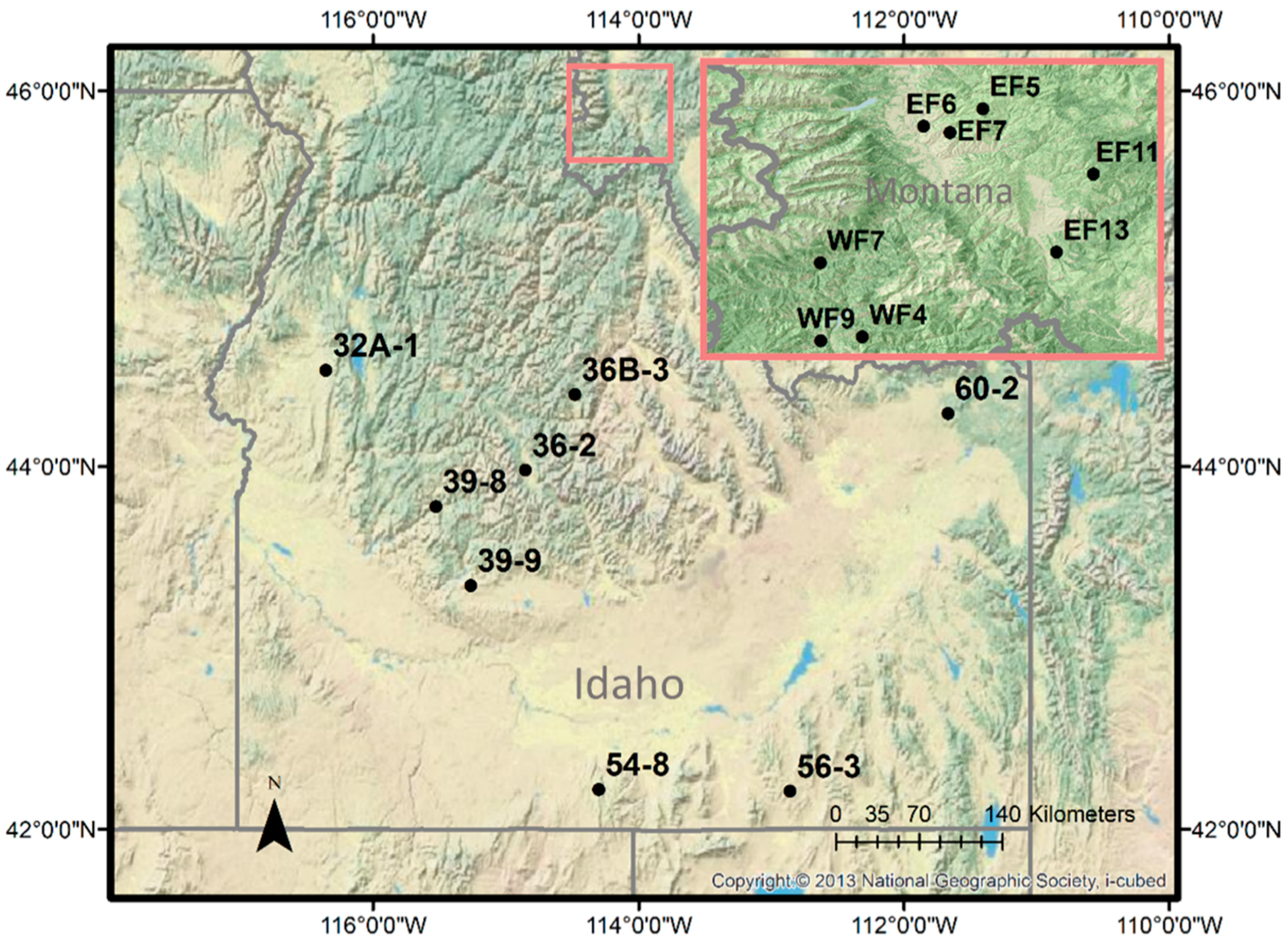
We used digital camera data from two adjacent study areas, one in southwestern Montana and the other in Idaho. The Idaho camera network consisted of eight sites spread across an extensive geographic area of 185,000 km
2 in central and southern Idaho (
Figure 1). The Montana camera network consisted of eight sites in the Bitterroot valley of Montana (
Figure 1). For the Montana study area, eight camera sites were placed within a 1900 km
2 study area to demonstrate intensive monitoring of a smaller geographic area.
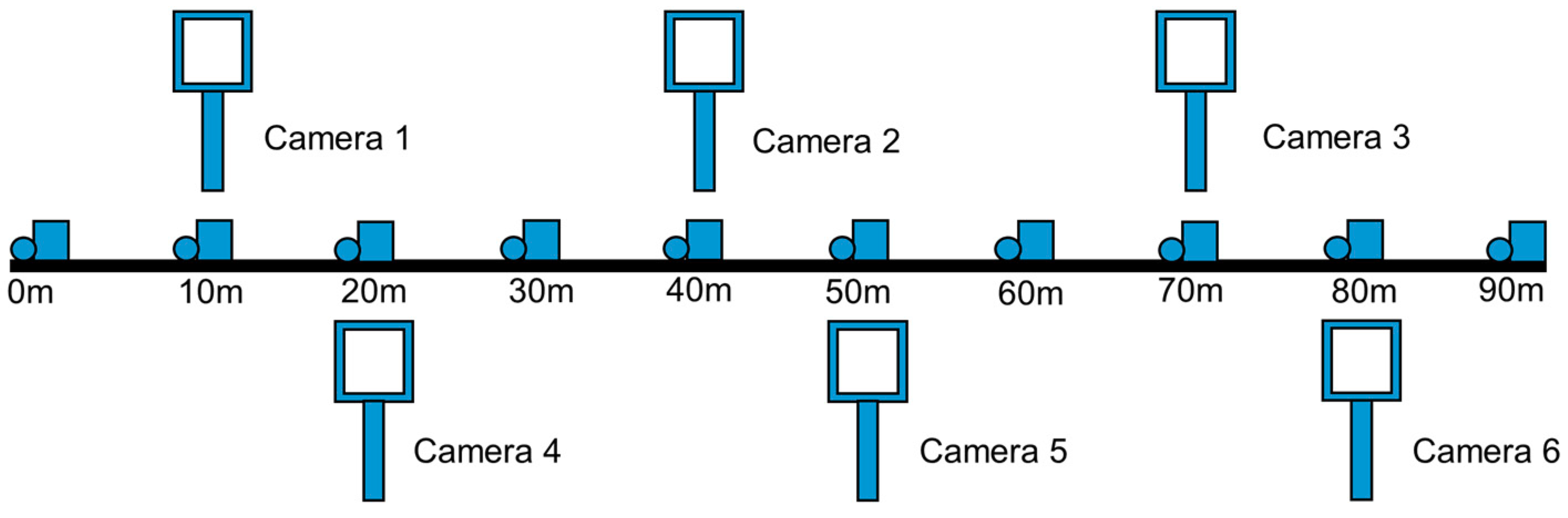
Camera sites were the observational units for this study. Between 4 and 6 cameras were placed approximately 1 m above the ground along transects at each site to capture the vegetation composition for in-situ observations. Multiple camera along each transect were used to capture a larger observational footprint than a single camera and to provide the appropriate scaling to the 250 m MODIS NDVI pixel. Multiple cameras on a site also provide redundancy to reduce the impact of camera failures.
Sites were defined as the area within 250 m of the 100 m transect lines and were spatially located with global positioning system (GPS). The area defined as the site was generated by creating a 250 m buffer around transect lines within a geographic information system (GIS). In the field ocular estimation, rangefinders and measurement tapes were used to define the site area. Due to the range of cover conditions, sites were classified into three basic categories based upon the presence of forest canopy. Those categories were forested, rangeland and mixed canopy. Forested sites had forest cover across the entire site, rangeland had no forest cover on the site or within 25 m of the edge of the site. Mixed canopy sites had forest cover on the site or within the 25 m buffer around the site. The categorization method was done in two stages: Through ocular estimates upon site visits and by manually observation of sites using site locations and 2013 National Agricultural Imagery Project (NAIP) imagery, a 1 m resolution imagery product.
Previous studies demonstrated that there are different relationships between canopy measures of NDVI and understory dynamics [
26]. This study’s cameras were placed in open rangelands in Idaho, where there would be no over-story canopy. Sites in the Montana study area were located in forested and mixed canopy as well as rangeland sites. At the forested and mixed canopy sites, we expected the differences in vegetation covers to significantly affect the correlation between in-situ camera data and satellite NDVI data due to the inclusion of over-story vegetation within MODIS NDVI pixels.
2.2. Plant Phenology Camera Sampling Design
In both study areas, digital cameras were installed along 100 m vegetation survey transects running east to west using TimelapseCam 8.0 cameras built by Wingscapes in Birmingham AL, USA. Cameras were placed in 15–30 m increments along the transect with half of the cameras placed north of the transect and half placed south of the transect, all cameras looking north (
Figure 2). In the Montana study area cameras in the rangeland and mixed canopy sites were mounted on metal stakes 1 m above the ground while forested plot cameras were mounted to trees the same distance above the ground. Cameras were placed in early 2013 before most snowmelt occurred in the study area. The daily timing of photographs was variable; many cameras took photos at 11:00 and 16:00 mountain standard time (MST) for the first few months of the season and then shifted to three daily photos at 11:00, 13:00 and 16:00 MST until the end of the season. The resulting dataset consisted of 49 cameras on 10 sites producing over 23,000 images for the Montana study area.
The Idaho study area had only grass and shrub dominated rangeland sites. The rangeland sites in both study areas were selected based on their vegetation homogeneity for at least 250 m around the site to reduce the likelihood of having a MODIS NDVI pixel with mixed cover types at those sites. Starting in 2014, Idaho site cameras took photos over the winter to record the start of the next year’s growing season. After removing malfunctioning and unusable camera data, the Idaho camera network consisted of 26 cameras on six sites in the year 2014 and 31 cameras on eight sites in 2015 producing over 41,000 images.
2.3. Processing Phenological Indices
Camera data consist of multiple daily digital photos from a constant field of view over a growing season. Photo data from all cameras were manually reviewed. Changes in camera view, photo timing, and camera damage were noted and cameras were assigned condition codes of usable, marginal, or unusable based upon the condition of the photo data. Regions of interest (ROI) identifying vegetated areas were created for each camera as separate shapefiles within ArcGIS. Site ROI were created to cover most of the vegetative area within the field of view of each camera while limiting debris such as site markers, fences and vegetation greater than 1 m above the ground.
To extract phenology data from digital camera photos, previous studies often created their own custom programs in a variety of software platforms [
11,
15,
17]. By far, the most common software used to extract data from digital photographs in the literature is the Phenocam Image Processor, a proprietary MATLAB-based software developed for the phenocam network [
27], and its equivalent R package ‘Phenopix’ [
28].
For our study we built and incorporated a photo analysis tool as part of the RMRS Raster Utility ArcGIS Add-in toolbar [
29]. Information regarding the photo analysis tools installation, and implementation are available online [
30], along with the tool’s source code [
31]. The tool and the color indices we used assume the digital imagery is in a red/green/blue (RGB) color scheme, where every color is defined as a combination of pure red, green and blue light. Each pixel in an image has a value in each of these three color bands referred to as the digital number (DN) that ranges from 0 (no brightness) to 255 (maximum brightness). The tool extracts the mean DN from each of the three color bands of an image within the ROI. DN mean values are then used as inputs into equations developed to quantify aspects of greenness and phenological phase changes from visual spectrum data. These equations are commonly used to summarize red, green, and blue (RGB) portions of the electromagnetic spectrum and correlate index values to phenology [
11,
16,
32,
33,
34,
35]. The color indices used in our study include: Green chromatic coordinate (GCC) [
36], excess green index (ExG) [
37], and the normalized difference of the green and red bands (VIgreen) [
38].
where G = mean green DN, R = mean red DN, B = mean blue DN for the ROI.
The GCC and ExG indices are designed as measures of greenness to overall image brightness [
36,
37]. The VIgreen index was developed to mimic NDVI values using the visual green band in place of the near-infrared band from the NDVI formula [
38].
Our NDVI data was extracted from the MODIS NDVI pixels that contained our study site locations for the year’s corresponding to our camera network data. Cloudy pixels in this dataset were defined using the data’s pixel reliability layer and were interpolated using methods from Reference [
39].
2.4. Statistical Analysis
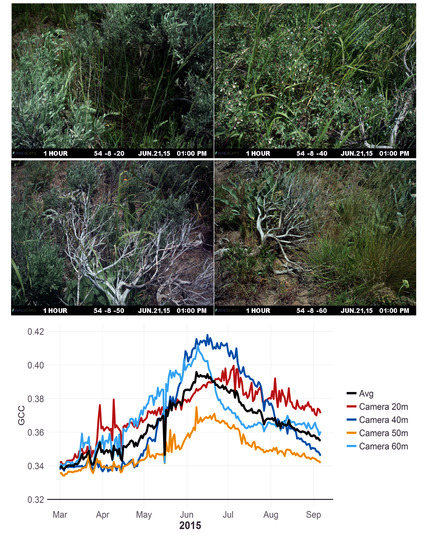
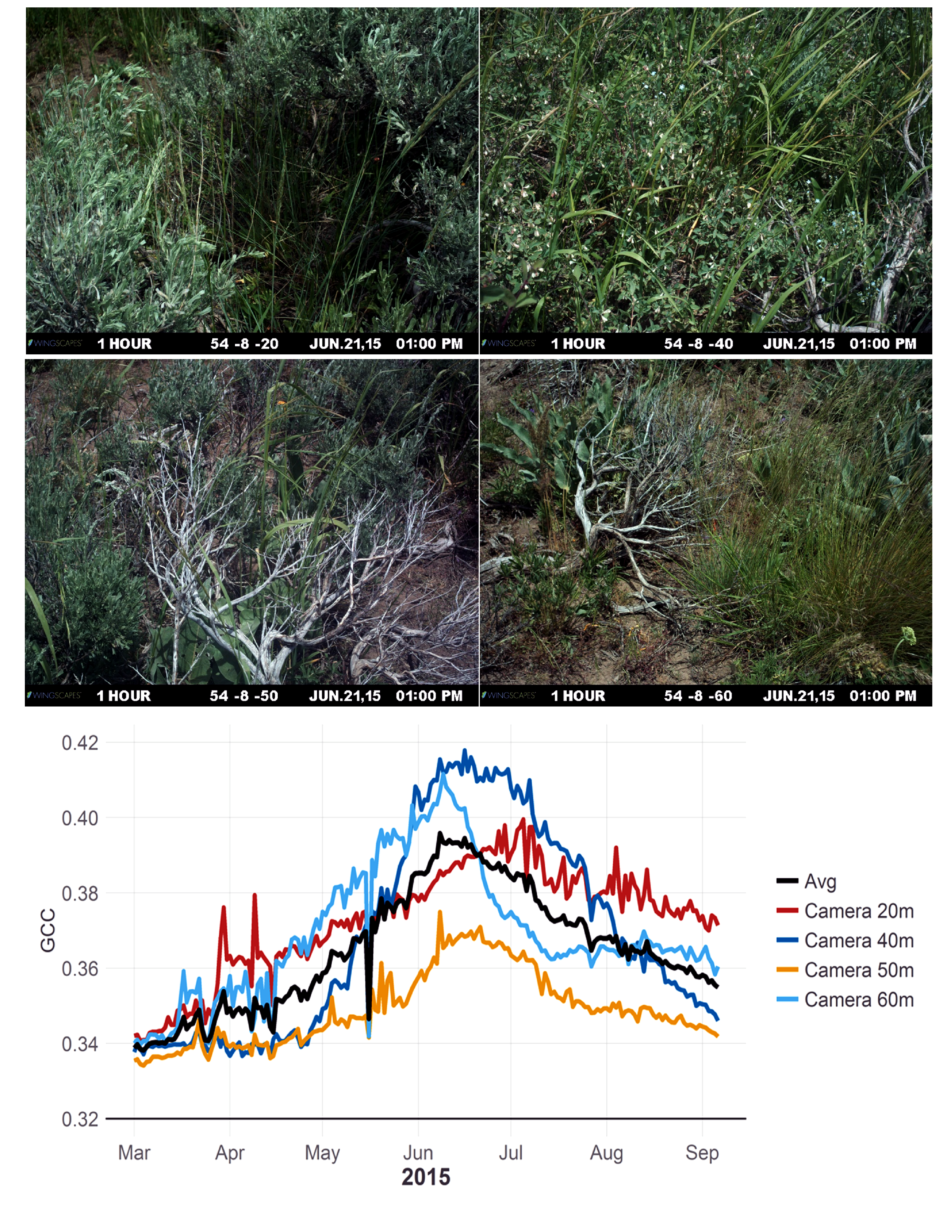
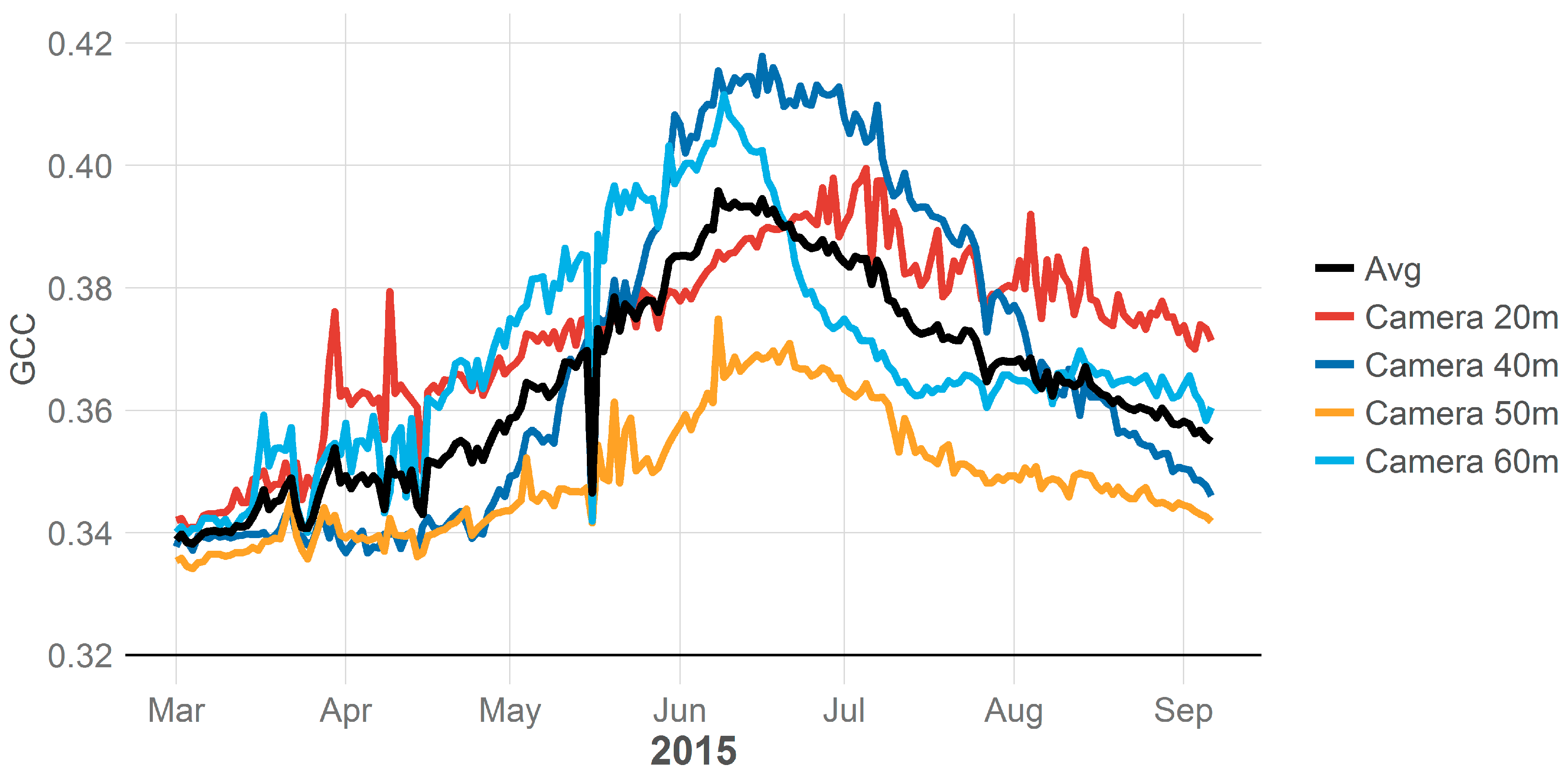
Our photo analysis tool outputs a text file that includes the mean values of the red, green and blue bands from the digital photo, three camera phenology indices from Equations (2)–(4) (GCC, ExG, VIgreen) as well as the total of the red, green and blue bands (RGB) as measure of the average brightness of the photo. To limit the effect of cloud shadows and weather events within our camera data, we selected the photo with the highest brightness (RGB) value to represent the daily values for a camera. We then scaled up to the site level by averaging daily data from multiple site cameras to produce site level phenology values for each day (
Figure 3).
The MODIS NDVI data is a composite of the best available pixel values from all the daily MODIS images within a 16-day period [
21]. This can lead to multiple temporal interpretations of MODIS NDVI data. Therefore, in our study NDVI values were assigned to the midpoint of the 16-day period to represent a temporal smoothing of the MODIS NDVI data and to the actual day in which camera data was acquired. In our analyses we compare, both temporal representations of the MODIS NDVI data.
The MODIS NDVI and the three camera indices values were normalized using feature scaling to bring all values into a range of zero to one, representing the index’s minimum and maximum values. Normalizing the indices facilitated comparison between indices with differing units and scale. Temporally the MODIS NDVI actual day of observation within the MODIS NDVI 16-day periods were compared to each of the camera indices average daily values for the same 16-day period and the camera indices day of observation value using Pearson’s correlation coefficient.
We developed phenology curves based on the camera and satellite indices to compare phenological dates. This was achieved by smoothing daily camera indices and 16-day NDVI data using fourth-order polynomial regression models fit to each index at each site [
22,
40]. For example, for site 32A1, the GCC fourth-order polynomial equation is:
We estimated the start of season (SOS) date for the eight Idaho sites in the year 2015 and five of the Montana sites using the half-maximum approach. This approach uses the annual minimum and maximum values of the fourth order polynomial regression models to calculate a midpoint for the green-up value. This method was designed for modelling deciduous forest leaf expansion. We used it in our analysis of sites dominated by grasses and shrubs because it is site and index specific allowing us to compare across sites without adjusting for differences in the camera, site composition, or index [
41]. Date of maximum (MAX) was identified as the peak of our modeled vegetation indices. We were unable to estimate SOS and MAX dates for three of the Montana sites, and year 2014 sites in Idaho because cameras were placed too late on those sites to capture the start of the growing season. We were also unable to estimate end of the growing season dates due to camera removals before senescence was complete for those same locations.
3. Results
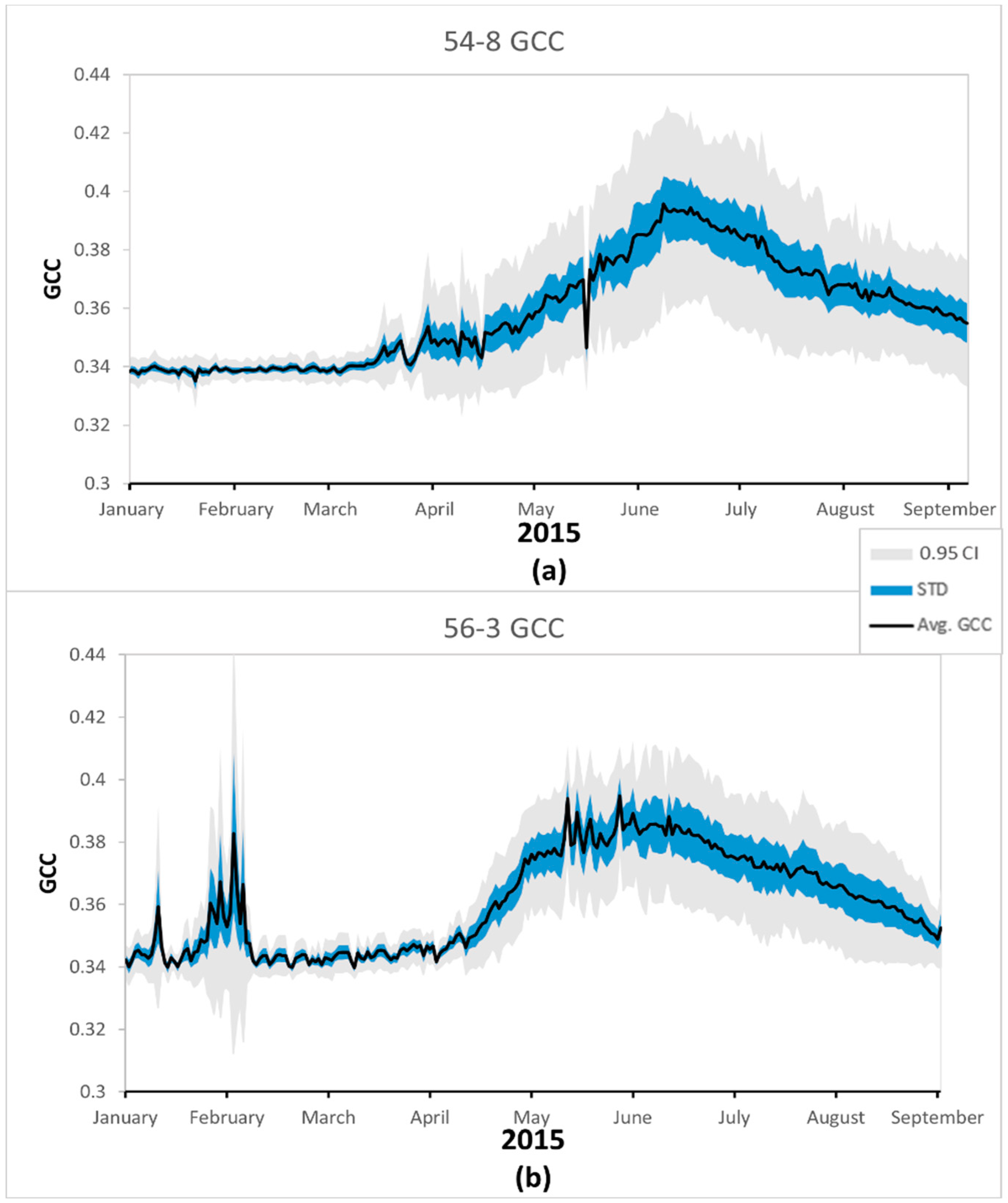
The between camera variability within a site was affected by the small number of cameras on a site and their field of view. Sites where more cameras returned usable data had generally higher variability but smaller confidence intervals when compared to sites with few cameras,
Figure 4. Across sites and camera indices the variability and uncertainty of averaging cameras followed a similar pattern of low variability and uncertainty during the dormant season and discreet weather events within the growing season and higher variability and uncertainty during the growing season, typified in
Figure 4.
The results of our site-level comparisons show that in the Idaho study area, the ExG and GCC camera index values were highly correlated to MODIS NDVI (Pearson correlations of 0.80 to 0.95, respectively), while the VIgreen camera index had the lowest correlation to MODIS NDVI (
Table 1). Averaging data from multiple cameras per site smoothed the digital camera derived phenology indices and improved its correlation with MODIS NDVI (
Figure 3). The 16-day mean DN values for camera indices were not significantly different (α = 0.95) from using the daily camera value for the corresponding MODIS NDVI date, and did not consistently improve or decrease the correlation results across sites. Thus, the following results were based on averaging the daily camera data into 16-day MODIS periods.
The high correlation between camera and MODIS NDVI at Idaho rangeland sites suggest that the camera indices are capturing the same vegetation green up signals as MODIS NDVI. The uniform results from the Idaho study area reflect the site selection of rangeland ideally suited for correlation with satellite observations. In contrast, the Bitterroot sites were much more variable than the Idaho sites (
Table 1,
Figure 1). This variability is most likely a function of the mixed cover types, number of 16-day periods observed, and the number of cameras on a site. Only one Bitterroot study area site (EF6) was a rangeland site of homogenous open grass and shrub land across the entire 250 m MODIS pixel extent, and it had the highest correlation with MODIS NDVI (R = 0.855). The four forested and five mixed canopy sites have varying levels of correlation (
Table 1).
Start of season dates estimated from MODIS NDVI were earlier than the digital camera indices estimates in all but two sites (
Table 2). The exceptions were sites EF5 and EF11, a mixed canopy and forested site respectively, where the camera indices were not significantly correlated to MODIS NDVI (
Table 1). The estimated day of maximum greenness (MAX) correlated well between NDVI and the camera indices. The differences in the frequency of observations between the camera indices (daily) and NDVI (16-day) should be considered when interpreting these results. Overall, the camera indices had consistently shorter estimates of the amount of time from start to maximum growing season than MODIS NDVI (
Table 2).
When phenological dates were derived from the MODIS NDVI and compared to dates derived from the three camera indices there was substantial difference in the estimated start of season dates. The camera indices and MODIS NDVI estimates of day of maximum did not consistently estimate earlier or later MAX day for rangeland sites (
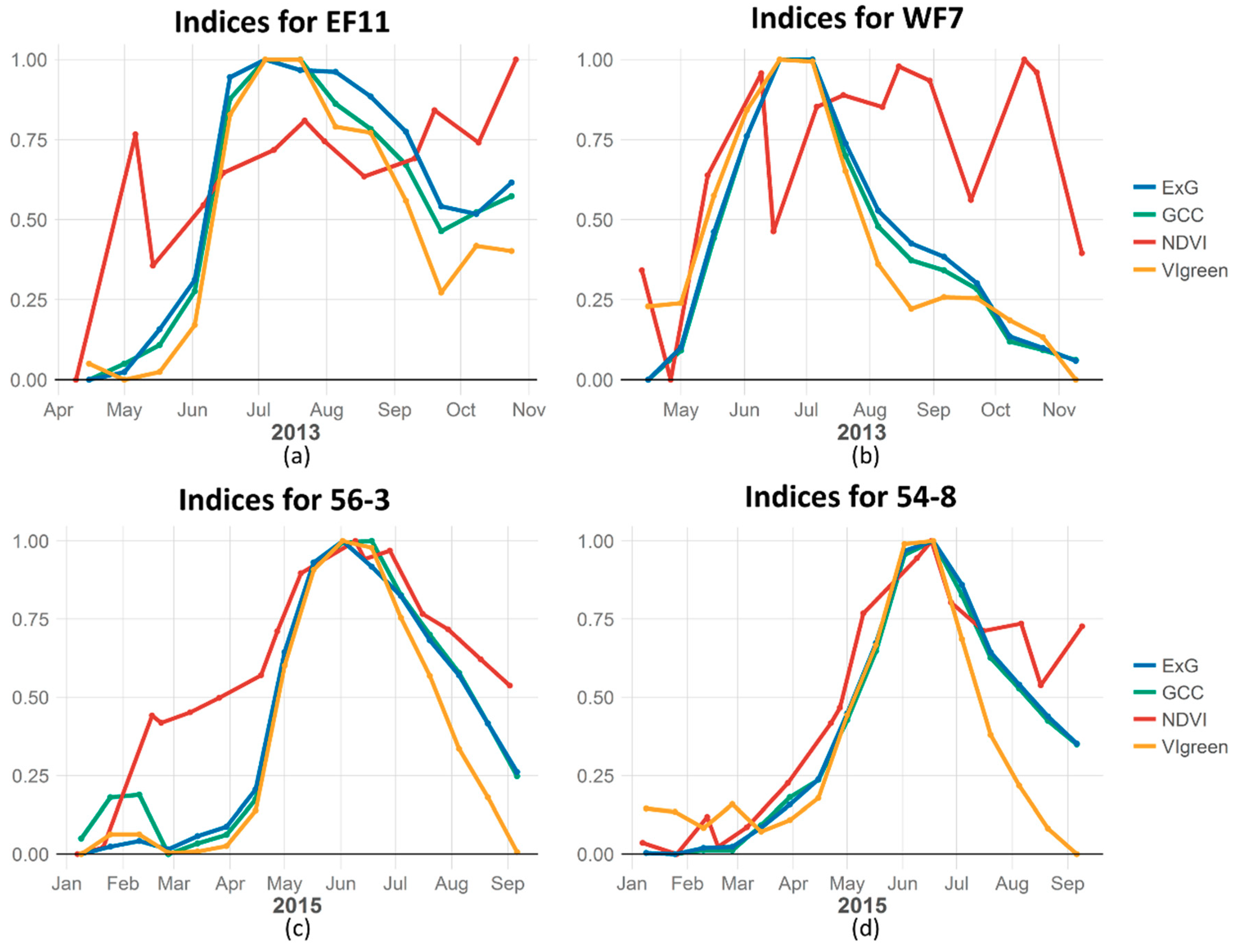
Table 2). Though not significant (α 0.95), the trends in the estimate MAX result suggests that at mixed canopy and forested sites MODIS NDVI consistently estimated a later MAX day then the camera indices. The MODIS NDVI values across sites started increasing earlier in the season and had a smoother ascent to the day of maximum than camera indices (
Figure 5).
Figure 5 visually compares the camera indices to MODIS NDVI vegetation indices across the growing season at four sites. The camera indices (GCC, ExG and VIgreen) are an average of 16 days of observations and therefore smoothed while the MODIS NDVI data is a single observation meant to represent 16 days, and will look more variable in comparison. To more accurately depict the real timing of the MODIS NDVI observations the NDVI values are plotted on the day the observation was taken, while the averaged camera indices are plotted at the middle day of the 16 day period in the figure.
Figure 5a,b are forested and mixed canopy sites respectively where the MODIS NDVI data, unlike the camera indices, observed all vegetation canopies at the site and not only the understory canopy. The lower correlation found between the VIgreen camera index and MODIS NDVI compared to the GCC and ExG index is primarily in the rapid decline of VIgreen in autumn (
Figure 5).
4. Discussion
Our results confirm that plant camera data can be effectively linked to moderate resolution remote sensing data using replication at the site level, even when individual cameras have a small field of view. We used a network of cameras, whereas most previous studies only used 1 plant camera per site [
21,
22,
23,
40]. Satellite-based vegetation indices such as the MODIS 16-day composite NDVI product are designed to be used at the landscape level as individual pixel accuracy can vary [
42]. As our
Figure 5a,b shows MODIS NDVI can become quite ‘noisy’ at the single pixel level in a heterogeneous landscape. At the scale of several hundred square meters a network of digital cameras will have the advantage of multiple temporal and spatial observations that can be masked to specific vegetation when compared to a single pixel from satellite data that can contain both vegetation and non-vegetated cover types.
Our study confirms, though that there can be strong correlations between digital camera and MODIS NDVI data. This correlation is increased when observing homogeneous rangeland vegetation sites (
Table 1 and
Table 2). The correlation between the VIgreen camera index and MODIS NDVI was not as strong as the other two indices we compared which was an unexpected result given that Vlgreen was designed to resemble NDVI [
38] and a recent study found the opposite result [
43].
One reason for this discrepancy might be due to the rapid decline of VIgreen in autumn when compared with MODIS NDVI (
Figure 5). VIgreen is a ratio of red to green colors in an image (Equation (4)) and is therefore more sensitive to changes in the amount of red in an image brought on by vegetation senescence, than GCC and ExG. The VIgreen index due to its color combination could be a superior measure of the onset of senescence but unfortunately in our study we were unable to extract an estimation of the date of senescence due to the timing of camera removals. We used a fourth order polynomial for our smoothing method as previous studies [
44] found no single smoothing method consistently superior for deriving land surface metrics from MODIS NDVI data.
When estimates of SOS and MAX day were derived from the indices we found a consistently earlier estimate of SOS day from MODIS NDVI compared to the camera derived indices. This result of shorter green-up period between start of season and max of season time in our camera indices are consistent with several previous studies that compared MODIS data to in-situ camera indices [
20,
21,
22,
23]. The Bitterroot sites that had derived phenological dates from either mixed or forested canopy all showed later estimates of MAX days from MODIS NDVI than the camera indices. This result could be due to the phenology of the overstory having a longer growing seasons than the understory, but the sample size is too small to draw conclusions from this result. To address questions of the magnitude and consistency of the differences in deriving phenological dates from in-situ camera and MODIS data future studies should have a larger sample sizes. The use of ground crew estimations such as in Reference [
21] would also add to the comparison.
Some studies have suggested earlier understory development [
45], large topographical differences within pixels [
46], or a result of differences in the observational spatial and temporal scales [
20] explain earlier start of season trend in MODIS products when compared to camera indices. Earlier understory development would not explain the differences in our rangeland sites that have no forested canopy, however, rangeland species composition my not be comparable to understory vegetative species composition making it difficult to compare the two categories. While some of our sites were in a mountainous terrain our study design would be expected to capture topographical differences in a site. Further investigation is required to understand the precise mechanisms driving these differences.
At closed canopy forested sites, camera observations were of the understory vegetation, while satellite observations of those sites are of the forested canopy. We did not expect those data to be highly correlated as they observed two different vegetation strata, though they occupy the same spatial footprint. There were also a few mixed canopy sites, where camera data was in a rangeland area while the MODIS NDVI pixel covered the rangeland area as well as nearby forested areas leading to a mixed pixel effect [
5,
46]. As expected there was much less correlation at mixed and forested canopy sites (
Table 1 and
Figure 5a,b). The degree to which the phenological signal is a mix between vegetation types is the likely cause of the difference in correlations between those MODIS pixels and our camera data, for example MODIS NDVI pixels with less forest will have higher correlation to our camera indices that only observed non-forested vegetation greenness, than pixels that contain more forested areas. In our forested sites MODIS data captured reflectance of the top of the forest canopy while ground based cameras in that area observed reflectance of the understory, leading to the low correlations between our datasets at those sites given that the indices were not observing the same vegetation.
The noisy NDVI result may be related phenology of mid-level canopy (i.e., tall shrubs) important to MODIS NDVI but not captured by cameras focused on vegetation under 1 m in height. The timing of bud burst and leaf abscission in the mid canopy will often not coincide directly with phenology of ground-level herbaceous plants. The intermountain regions of Idaho and Montana will often experience a fall regrowth of grasses in October, providing a second green-up period for the understory during leaf senescence, but prior to abscission, NDVI will decrease, only to increase after leaves fall as the herbaceous understory becomes visible. The different phenology between these plant groups may cause NDVI to oscillate. These results suggests that the use of MODIS NDVI in forested sites as a direct substitute for evaluating understory phenology may not work well. Care should be taken when NDVI derived from satellites like MODIS is used to estimate understory vegetation phenology in forested and mixed forested areas. Alternatively, to quantifying the reflective contributions of the understory canopy in some sparsely forested areas one can use the method suggested by Reference [
47] that has found some success [
48]. Future studies could use in-situ digital cameras to quantify the amount of forest to understory canopy, their individual reflectance contributions and the temporal changes in those contributions through a growing season.
The weak correlation in vegetation phenology between our camera and satellite data from closed forest canopy and mixed canopy sites highlight the advantage of digital cameras for phenological observations at finer spatial scales. The spatial resolution of digital cameras allow for the flexibility to quantify the phenology of multiple cover types through the placement of cameras and creation of ROIs within a camera view [
12]. Other publicly available remotely sensed data sources have a finer spatial resolution than MODIS, such as LANDSAT or Sentinel. However, what those imagery systems gain in spatial resolution they give up in temporal resolution and are still limited to a top down view of the canopy.
The level of uncertainty and variability when averaging camera data across a site is affected by the number of cameras that are being averaged and their field of view. While sites and transects in this study were selected for the homogeneity of their plant groups the loss of a camera on a site that had different phenological trends then other camera at that site, such as Camera 20 m in
Figure 3, could substantially change the sites phenological trend. However, here, we used between 3 and 5 cameras at each site, yet,
Figure 4 demonstrates that even with the uncertainty in phenological indices (i.e., GCC in
Figure 4), we would still be able to extract phenological parameters—and their uncertainty—at each site. Future work should look to increase the number of cameras on a site or quantify the plant assemblage within a site to verify that it matches the plant assemblage within the camera views. This could consist of taking a general census of plant cover across the site. Then ROIs for each plant species within a camera view could be created to extract phenology indices for plant species. The plant species indices could then be combined across cameras and weighted by the entire sites plant cover. This methodology of a weighted average could see improved phenology estimation for a site over the unweighted averaging of camera indices used in this study.

 ,
, 


