Article

A New Methodology for Estimating the Surface Temperature Lapse Rate Based on Grid Data and Its Application in China

1
Department of Atmospheric Science, School of Environmental Studies, China University of Geosciences, Wuhan 430074, China
2
Laboratory for Climate Studies, National Climate Center, China Meteorological Administration, Beijing 100081, China
3
School of Resource and Environmental Sciences, Wuhan University, Wuhan 430079, China
*
Author to whom correspondence should be addressed.
Remote Sens. 2018, 10(10), 1617; https://0-doi-org.brum.beds.ac.uk/10.3390/rs10101617
Submission received: 6 July 2018 / Revised: 20 September 2018 / Accepted: 9 October 2018 / Published: 11 October 2018

Abstract

:
Land surface temperature (LST) is an important parameter in the study of the physical processes of land surface. Understanding the surface temperature lapse rate (TLR) can help to reveal the characteristics of mountainous climates and regional climate change. A methodology was developed to calculate and analyze land-surface TLR in China based on grid datasets of MODIS LST and digital elevation model (DEM), with a formula derived on the basis of the analysis of the temperature field and the height field, an image enhancement technique used to calculate gradient, and the fuzzy c-means (FCM) clustering applied to identify the seasonal pattern of the TLR. The results of the analysis through the methodology showed that surface temperature vertical gradient inversion widely occurred in Northeast, Northwest, and North China in winter, especially in the Xinjiang Autonomous Region, the northern and the western parts of the Greater Khingan Mountains, the Lesser Khingan Mountains, and the northern area of Northwest and North China. Summer generally witnessed the steepest TLR among the four seasons. The eastern Tibetan Plateau showed a distinctive seasonal pattern, where the steepest TLR happened in winter and spring, with a shallower TLR in summer. Large seasonal variations of TLR could be seen in Northeast China, where there was a steep TLR in spring and summer and a strong surface temperature vertical gradient inversion in winter. The smallest seasonal variation of TLR happened in Central and Southwest China, especially in the Ta-pa Mountains and the Qinling Mountains. The TLR at very high altitudes (>5 km) was usually steeper than at low altitudes, in all months of the year.

1. Introduction

Temperature lapse rate (TLR) is the rate at which temperature decreases with altitude. Generally, there are two kinds of TLRs, dynamic and static TLR. The former describes the temperature change of the air parcel when it rises (e.g., dry adiabatic lapse rate); the latter indicates the temperature changes with space, which may be vertical (e.g., tropospheric free-air TLR) or along the earth’s surface with different altitudes. The focus of this article is the TLR along the earth’s surface, or lapse rate of land surface temperatures (LST).
LST is an important parameter in the study of the physical processes of land surface, which is frequently used in the fields of hydrological and meteorological models [1,2], agricultural and ecological monitoring [3,4,5], and urban heat island analyses [6,7,8]. Remote sensing technology provides a spatial continually-distributed LST, which is of benefit to the analysis of spatial variation when compared to the limited ground meteorological stations [9]. The lapse rate of LST reflects the spatiotemporal variation of the thermal processes of land surface and the difference of regional climate, which can be used for the study of mountainous climates and probably for regional climate change, especially in remote mountainous areas where observations from ground meteorological stations are lacking. For example, different land-surface TLR at different sides of a mountain may be related to the vertical zoning of vegetation, and a steep TLR may cause a rapid vegetational change in the vertical [10,11]. In addition, elevation-dependent warming in mountainous areas may result in a temporal change in the TLR, and the more rapid warming at high altitude may be related to the shallower land surface and near-surface air TLR [12].
Some studies have found that there is a strong relationship between the mean LST and mean near-surface air temperature [13,14,15,16], and the seasonal pattern of monthly mean land-surface TLR is very similar to that of the near-surface air TLR [17]. However, as the LST is influenced by the surface regime [18,19], the relationship between them is not always stable. However, many previous studies have focused on the near-surface air TLR, and studies of the land-surface TLR are rare. Therefore, it is necessary to examine the land-surface TLR as a complement in the study of climatology and climate change. To avoid confusion, a negative TLR has usually been designated when the temperature decreases with the increase of elevation, and a positive TLR has been regarded as the temperature vertical gradient inversion in a substantial body of literature [11,20,21,22,23,24].
Atmospheric temperature decreases with the increase of elevation in the troposphere, and the global average annual mean atmospheric TLR is about −6.5 °C/km [25], which is generally used as a reference for near-surface air TLR. However, varied values of annual mean near-surface air TLRs have been reported for different areas [21,22,26,27]. Pepin and Losleben [28] found that TLR was steeper at higher elevations, and Mokhov and Akperov [29] pointed out that TLR became shallower from a low latitude to the polar regions. In addition, the atmospheric temperature sometimes remains constant or even increases with elevation [30]. A temperature inversion is frequently found in winter [23,31,32]. The annual cycle of the TLR shows different seasonal patterns, with some steeper in summer and shallower in winter [21,23,33,34], some steeper in winter and shallower in summer [11], and others that are steeper in spring and shallower in later summer or autumn [35,36].
Linear regression is widely used to calculate the TLR of a small region based on observational data of meteorological stations [24,37]. For a large region, stations are usually divided into several groups and the TLR in each group is calculated separately [22,34,38], or aggregated through a moving spatial window, thus each station has a local TLR [39,40]. Regarding the grid data, linear regression [41,42] and moving window regression [20] have also been adopted, based on grid values. However, as the TLR calculated through linear regression depends strongly on the stations being considered, and the station distribution is usually denser at low altitude than at high altitude, the results obtained may represent the TLR of a low altitude than of the whole mountainous area. It is also notable that as the grouping methods are different, the stations being considered in a group are different, which may reduce the comparability of the research results. Due to the heterogeneous spatial distribution of stations, a moving window regression cannot avoid the statistical errors caused by different sampling size or scales [43]. Though a linear regression, based on the grid data, eliminates the influence of heterogeneity, low correlation coefficients may be obtained, especially for the case of winter with enhanced temperature-inversion effects [21]. As for the identification of the seasonal pattern of a TLR, a line chart can tell the seasonal variation in a mountainous area or large scope, but cannot describe the details of a small scope with the effect of microclimate.
In this paper, we developed a methodology to calculate and analyze the TLR based on grid data, and used China as a case study for the application of the methodology by using grid datasets of moderate-resolution imaging spectroradiometer (MODIS) LST and digital elevation model (DEM). To be specific, we derived a formula on the basis of the analysis of the relationship of the temperature field and the height field, applied the image enhancement technique to calculate the gradient, and used the fuzzy c-means (FCM) clustering method to identify the seasonal pattern of the TLR. The analysis results were broadly in accordance with previous studies based on meteorological stations, which would form a reference to the study and application of both land-surface TLR and near-surface air TLR, in a large region with complex topography.

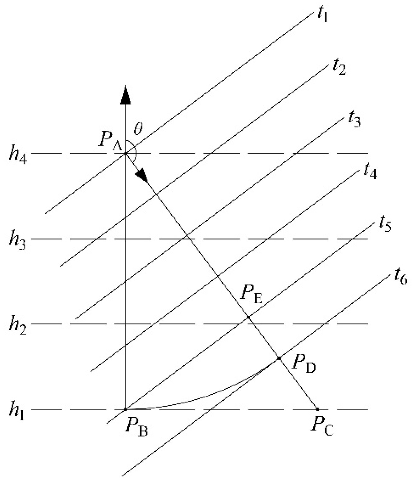
2. A Conceptual Framework

For a continuous, spatially-distributed height field and temperature field, the gradient of the height points to the direction that the variables increase at the greatest rate [44,45,46], i.e., the steepest terrain slope. However, the direction may not be the same as the direction in which the temperature decreases at the greatest rate (the gradient of temperature). Generally, there is an angle between them; an angle greater than π / 2 indicates that temperature decreases with the increase in height, and less than π / 2 indicating that temperature increases with the increase in height, i.e., the temperature vertical gradient inversion, and an angle equal to π / 2 indicates an unchanged temperature, with the increase in height. In a small region (compared with the average area covered by one meteorological station), the rate of change of height or temperature along a given direction can be considered to be constant, approximately, due to the continuously-varied terrain and the same atmospheric factors affecting the climate. Hence, the increase in temperature along the direction of the steepest topographical slope is the directional derivative of temperature, along the direction of the gradient of height at a site, i.e., the increase of temperature within a small region is the length of the gradient of temperature in the direction of the gradient of height.
For example, the angle between the gradient of height and the gradient of temperature, θ > π / 2 , shows a negative correlation between height and temperature (Figure 1). Within a given small scope of a distance between P A and P B (denoted as d P A P B ), the TLR is the difference of temperature, divided by the difference of height, i.e., TLR = t 1 t 5 h 4 h 1 . The length of the gradient of height at this scope is h 4 h 1 , and the length of the gradient of temperature is t 6 t 1 . In a homogeneous field, the difference of temperature between P A and P E , t 5 t 1 , is equal to d P A P E d P A P D · ( t 6 t 1 ) , where d P A P E = d P A P B · cos ( π θ ) . As d P A P B is equal to d P A P D , the TLR can be written as ( t 6 t 1 ) · cos θ h 4 h 1 , which is the length of the gradient of temperature divided by the length of the gradient of height, in the direction of the gradient of height.
In digital image processing, height field and temperature field are both discrete, and the gradient can be obtained through image enhancement techniques [47]. Three of the most common operators, Roberts, Prewitt, and Sobel, are used in edge-detection (a kind of image enhancement), and the Prewitt and Sobel operators are generally preferred to the Roberts [48]. As the Sobel operators implement differentiation in one direction and Gaussian averaging in the other, it makes for a smoother gradient and reduces the influence of noise.
Theoretically, temperature changes in a given cycle period. Hence, the TLR, which is decided by the gradient of temperature, also changes in the same cycle period as temperature. Hence, how the TLR changes with the seasons can be translated into two issues: (1) when the steepest (or shallowest) TLR occurs, i.e., where the wave trough (or crest) is, and (2) how much the magnitude of variability is within a year. To identify the variability model of TLR, four kinds of seasonal pattern were assumed, which were the steepest in spring, summer, autumn, and winter, respectively. However, the actual variability of TLR is usually characterized by more than one pattern. In order to identify which pattern it most likely belonged to and how much of it belonged to the pattern, the FCM clustering algorithm [49] was used. Furthermore, four standard samples generated artificially were added as a reference, which represented the typical seasonal patterns (the steepest in April, July, October, and January) in each season.

3. Materials and Methods
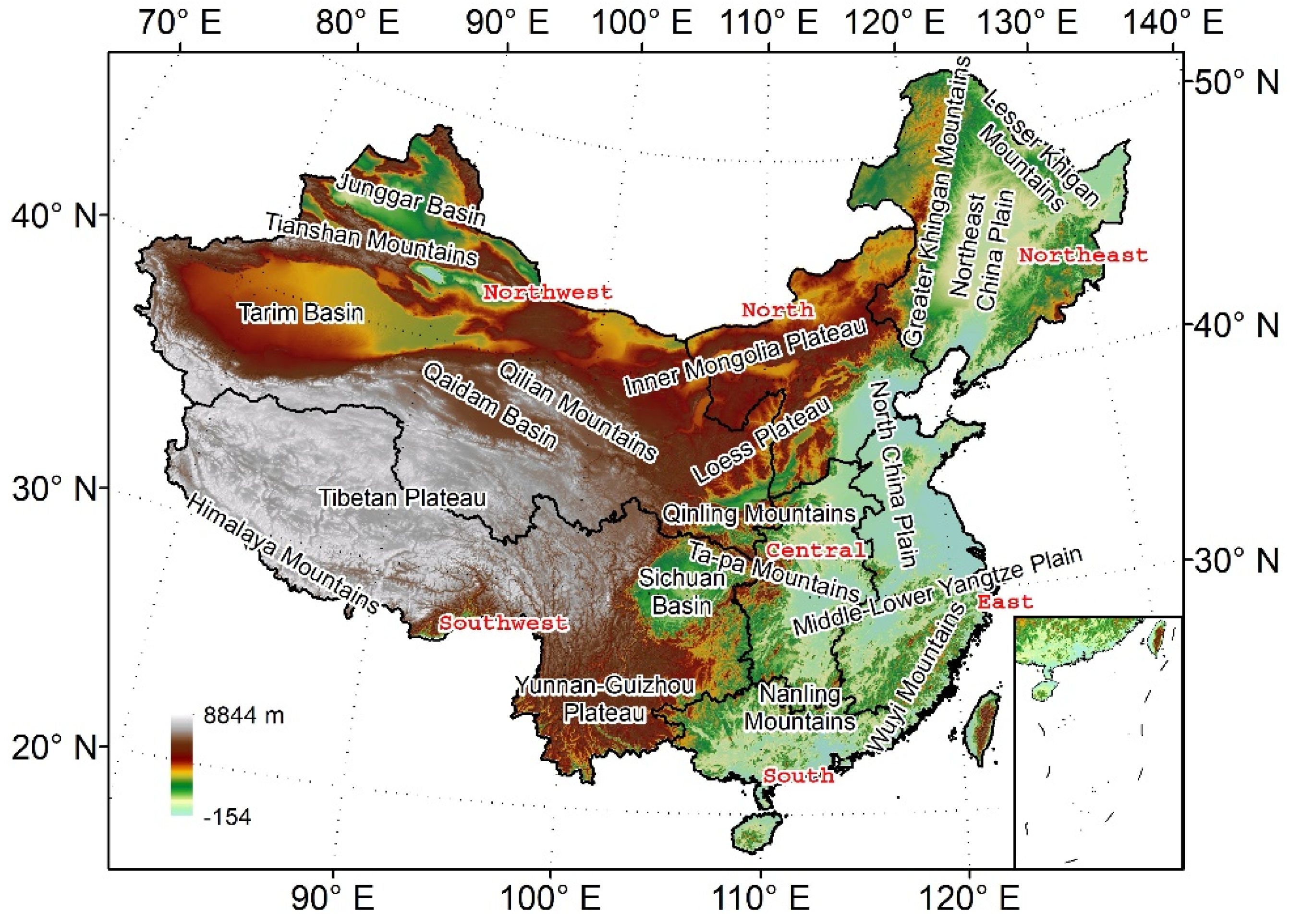
3.1. Data

The LST datasets were provided by the International Scientific & Technical Data Mirror Site, Computer Network Information Center, Chinese Academy of Sciences (http://www.gscloud.cn). The monthly mean LST was the average of the daily mean LST (average of diurnal and nocturnal LST) in each month, which was retrieved from MODIS data obtained by the satellite Terra and Aqua [9]. To avoid confusion, the mean LST above-mentioned is expressed as “LST” below. As there were a few missing values on the images, linear interpolation was used to fill the blank patches. These MODIS images were based on the geographic coordinate system of WGS-1984, at a spatial resolution of 0.0059° × 0.0059°. The range of the study area covered the whole of China, located from 4°00′N to 53°31′N latitude and from 73°40′E to 135°05′E longitude (Figure 2). The observed time ranged from January 2001 to December 2015. Monthly average LST was the average of the monthly LSTs of each month, from 2001 to 2015. Annual average LST was the average of the monthly average LST.
The dataset of DEM (GMTED2010) was provided by Natural Earth (https://www.naturalearthdata.com). The elevation data came from the DEM images, which were based on the geographic coordinate system of WGS-1984, at a spatial resolution of 30′ × 30′.
As the calculation of the TLR was based on both MODIS LST and DEM, they must have the same resolution. Hence, it was necessary to carry out resampling. When original images with a relatively high resolution were applied to a large-scale region, noise would seriously interfere with the accuracy of the judgment of the results, which might drown out the main information. In order to keep a balance between the denoising and maintaining the feature of the microclimate, resampling to a new spatial resolution of 10 km × 10 km (after projection) was undertaken in this case study.

3.2. Calculation of TLR

As LST is a function of space at a given time, its distribution throughout space is a scalar field (i.e., temperature field T ), and so is elevation (i.e., height field H ). The gradient of H at a site, denoted as H , is a vector pointing in the direction of the steepest slope at that site. Along this direction, the increase of temperature per unit of height is supposed to be the TLR. Hence, the TLR can be expressed as follows:
Γ = | T | · cos H , T   | H | ,
where T is the gradient of T and H , T is the angle between H and T . When the numerator and the denominator are both multiplied by | H | , Equation (1) can be written as follows:
Γ = T · H | H | 2 ,  
As MODIS images are based on the geographic coordinate system of WGS-1984, the distribution throughout space was on the surface of an ellipsoid, so the gradient could not be directly calculated through a computer. Equidistant cylindrical projection [50] was used to transform the surface of an ellipsoid into a plane, which simplified the complexity of calculation. Through this transformation, the pixels of the new image, denoted as T 0 , had the same distance along the longitudinal and latitudinal direction (10 km × 10 km). An extensional Sobel operator [51,52] of two 5 × 5 kernels,
O 1 = ( 1 2 0 2 1 4 8 0 8 4 6 12 0 12 6 4 8 0 8 4 1 2 0 2 1 ) ,   O 2   = ( 1 4 6 4 1 2 8 12 8 2 0 0 0 0 0 2 8 12 8 2 1 4 6 4 1 ) ,
were convolved with the image to calculate the gradient,
| T | = T x 2 + T y 2 ,  
α = atan ( T y T x ) ,  
where | T | and α are the length and the direction of T , respectively. T x and T y are the derivatives for x changes (longitudinal direction) and for y changes (latitudinal direction), which are calculated by
T x = T 0 O 1 / 960 ,  
T y = T 0 O 2 / 960 ,  
where denotes the two-dimensional signal processing convolution operation. The outside weights ([1,4,6,4,1] or [−1,−4,−6,−4,−1]) of each kernel are based on Pascal’s triangle, the coefficients of which are subject to a Gaussian distribution, and the inside ones ([2,8,12,8,2] or [−2,−8,−12,−8,−2]) are twice as much as them. As the center parts are given greater weights than the edge parts, the spatial relationship is a kind of impedance or a distance decay. The farther away a pixel is from the center, the smaller the impact it has on the TLR of the center pixel. Note that 960 is the product of the sum of the absolute of each element of a kernel ( i = 1 5 j = 1 5 | o i , j | ) and the size of each pixel (10 km), and the unit of gradient is °C/km. H , H x , and H y are calculated the same as T , T x , and T y .

3.3. Analysis of Seasonal TLR Variation

First, the standard score normalization, then unity-based normalization were carried out, based on the TLR. Four artificially generated standard samples, which shared the same cycle period (12 months) and held different phases ( { 0 , π , ± π 2 } indicating that the wave trough occurred in April, July, October, and January, respectively), were added to make the clustering. FCM was based on the minimization of the following objective function:
J M = i = 1 n j = 1 c u ij M r i c j 2 ,  
where M is the fuzzifier (= 1.01 here); n is the number of samples (including all non-void image pixels and four standard samples); c is the number of clusters (= 4 here); r i is the normalized TLR at the i th sample (which is a vector of 12 elements); c j is the center of the j th cluster; and u ij is the degree of membership of r i in the j th cluster. Note that r i c j is the norm expressing the similarity between r i and c j . Fuzzy partitioning is carried out through an iterative optimization of Equation (7), with the update of u ij and c j , which are expressed as follows:
u ij = 1 k = 1 c ( r i c j r i c k ) 2 M 1 ,  
c j = i = 1 n u ij M r i i = 1 n u ij M ,  
The sample i would be classified into the cluster with the largest u ij . The image pixels that shared the same cluster as any one standard sample, would hold a similar seasonal pattern to it. The magnitude of variability was measured by the range of the TLR, within a year.

4. Results of Case Analysis

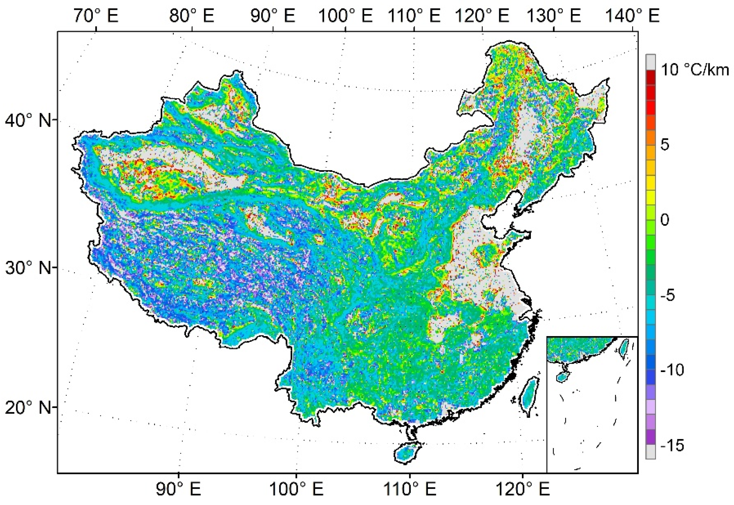
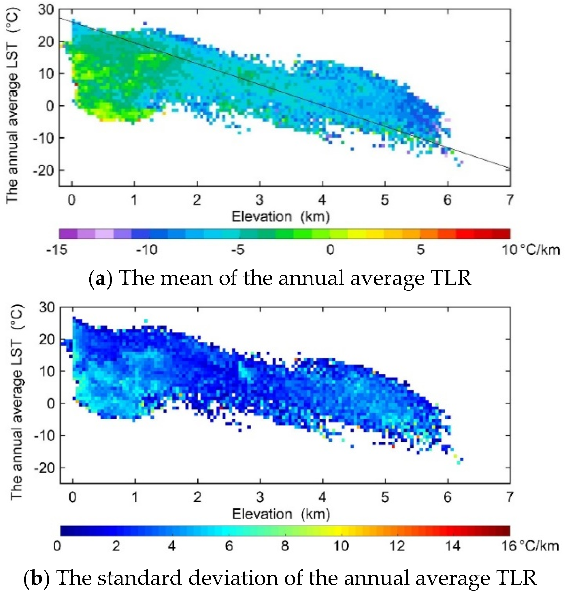
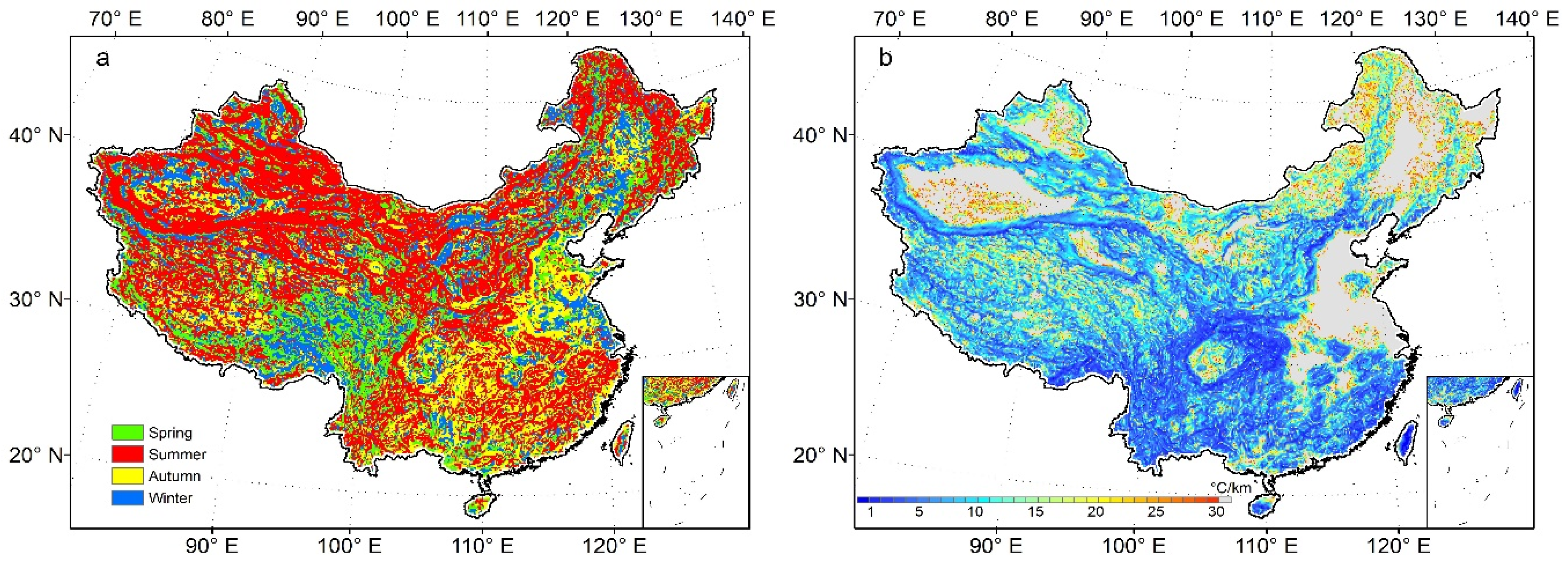
4.1. Spatial Variation of TLR

There were some areas with extremely small or large values of TLR ( Γ 15 or Γ > 10 °C/km), which were mainly located in the North China Plain, Northeast China Plain, and Tarim Basin (Figure 3). When leaving these areas out of consideration, the annual average TLR of Γ 0 °C/km accounted for 86.3%, indicating that the LST decreased with the increase of altitude, in most parts of China. The steep annual average TLR ( 15 < Γ 7 °C/km) mainly took place in the Tibetan Plateau. Temperature vertical gradient inversion ( 0 < Γ 10 °C/km) could be seen in some regions of Northeast, Northwest, and North China.
A big difference was found in the seasonal distribution (Figure 4 and Figure 5). The steep monthly average TLR mainly occurred in the Southwest (the percentage of image pixels with 15 < Γ 7 °C/km was greater than 20%, in all four seasons), Northwest (spring, summer, and early autumn), Northeast, and North China (summer and later spring) (Figure 5). The TLR of the mountainous and the hilly areas in Central, South, and East China became steeper (the percentage of image pixels with 15 < Γ 7 °C/km increased) in summer, and at the same time, the TLR of the Eastern Tibetan Plateau became shallower. The TLR of Eastern Tibetan Plateau became the steepest in later autumn and winter, but that of the western part of the plateau began to become shallow (Figure 4). The region-wide monthly average TLR of the Eastern Tibetan Plateau was shallower than the western part by about 1.6 °C/km, from June to September (Figure 6a,c). In winter, the temperature vertical gradient inversion was widely distributed in Northeast, Northwest, and North China (the percentage of image pixels with 0 < Γ 10 °C/km was greater than 20%) (Figure 5). It is notable that there was a temperature vertical gradient inversion in the western and northern parts of the Greater Khingan Mountains in Northeast China, in winter and in early spring, but a steep TLR occurred in some parts of the eastern slope of the mountains (Figure 4). The region-wide monthly average TLR of the Western and Northern Greater Khingan Mountains could be greater than 0 °C/km, in December and January, but those of the eastern slope of the mountains were much less than 0 °C/km, in the two months (Figure 6b,d).

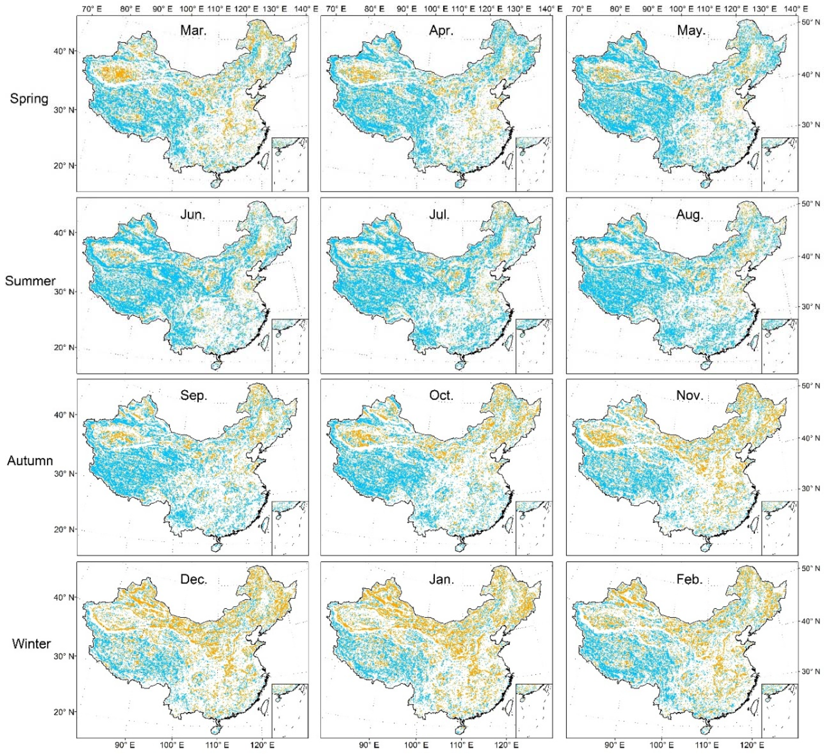
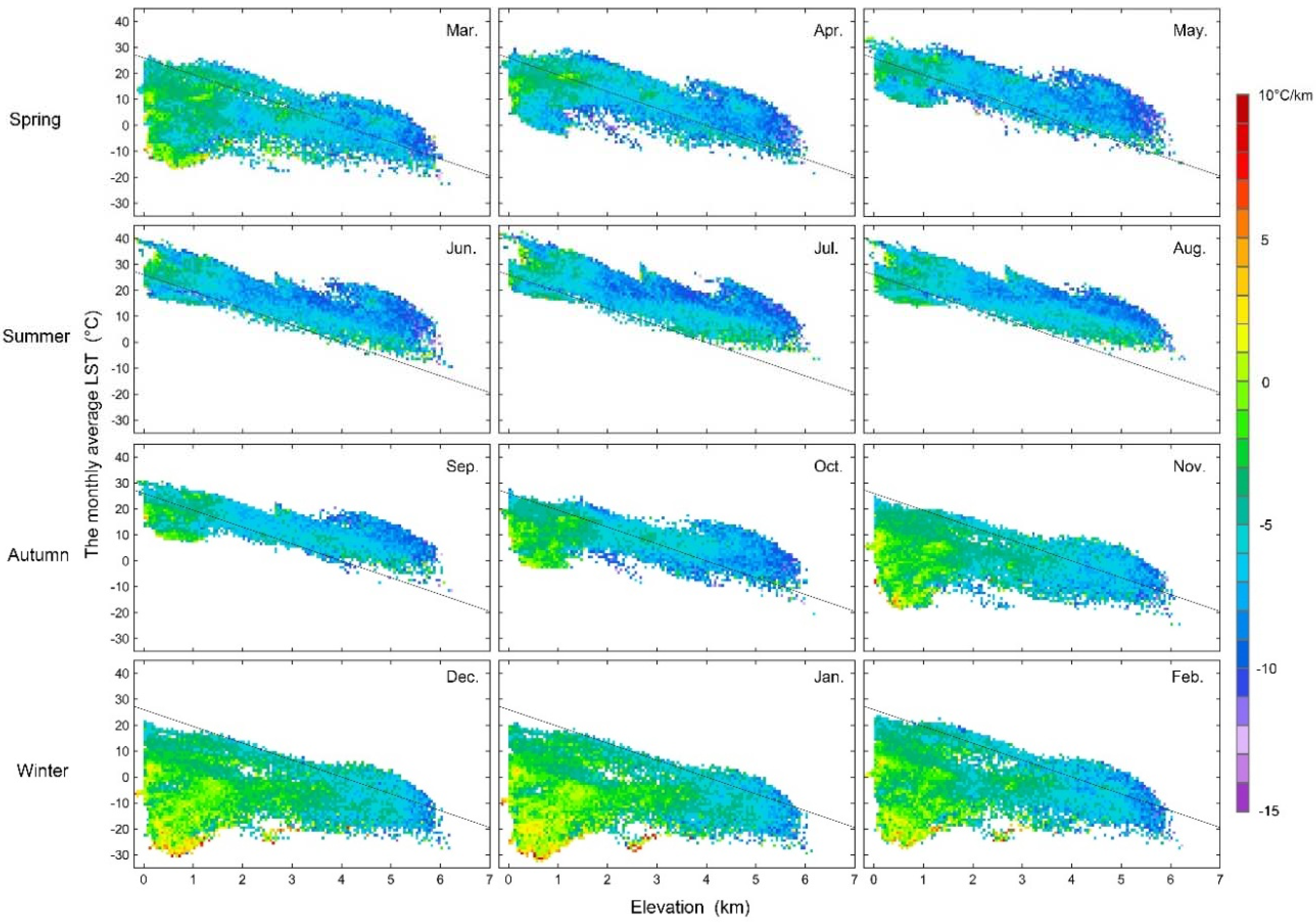
4.2. Temporal Variation of TLR

TLR is changeable in the areas of plains and basins with extremely small values of | H | (Figure 3 and Figure 4). However, the percentage of these areas ( Γ 15 or Γ > 10 °C/km) in each month was relatively stable (accounting for about 10%, respectively) (Figure 7). Based on this, this research focused on the other twenty-five levels of 15 < Γ 10 °C/km.
The country-wide monthly average TLR was steeper in summer than in winter (Figure 7). The spatial variability was larger in winter than in summer (standard deviation was 5.0 °C/km in winter and 4.5 °C/km in summer, data not shown). The percentage of predominant levels of Γ 0 °C/km was larger in summer than in winter. Meanwhile, there was an increased percentage of temperature vertical gradient inversion in winter, when compared to that in summer.
The monthly average TLR was roughly steeper at a higher altitude than at a lower one (Figure 8a), and was also generally steeper in summer than in winter, at a given elevation. Temperature vertical gradient inversion mostly happened at low altitudes, in winter. Though the monthly average TLR showed complex changes with an increase in LST, shallow TLR or temperature vertical gradient inversion also happened in winter (Figure 8b). Furthermore, strong temperature vertical gradient inversion could be found in winter, especially in December and January, at low elevations less than 0.2 km above sea level.

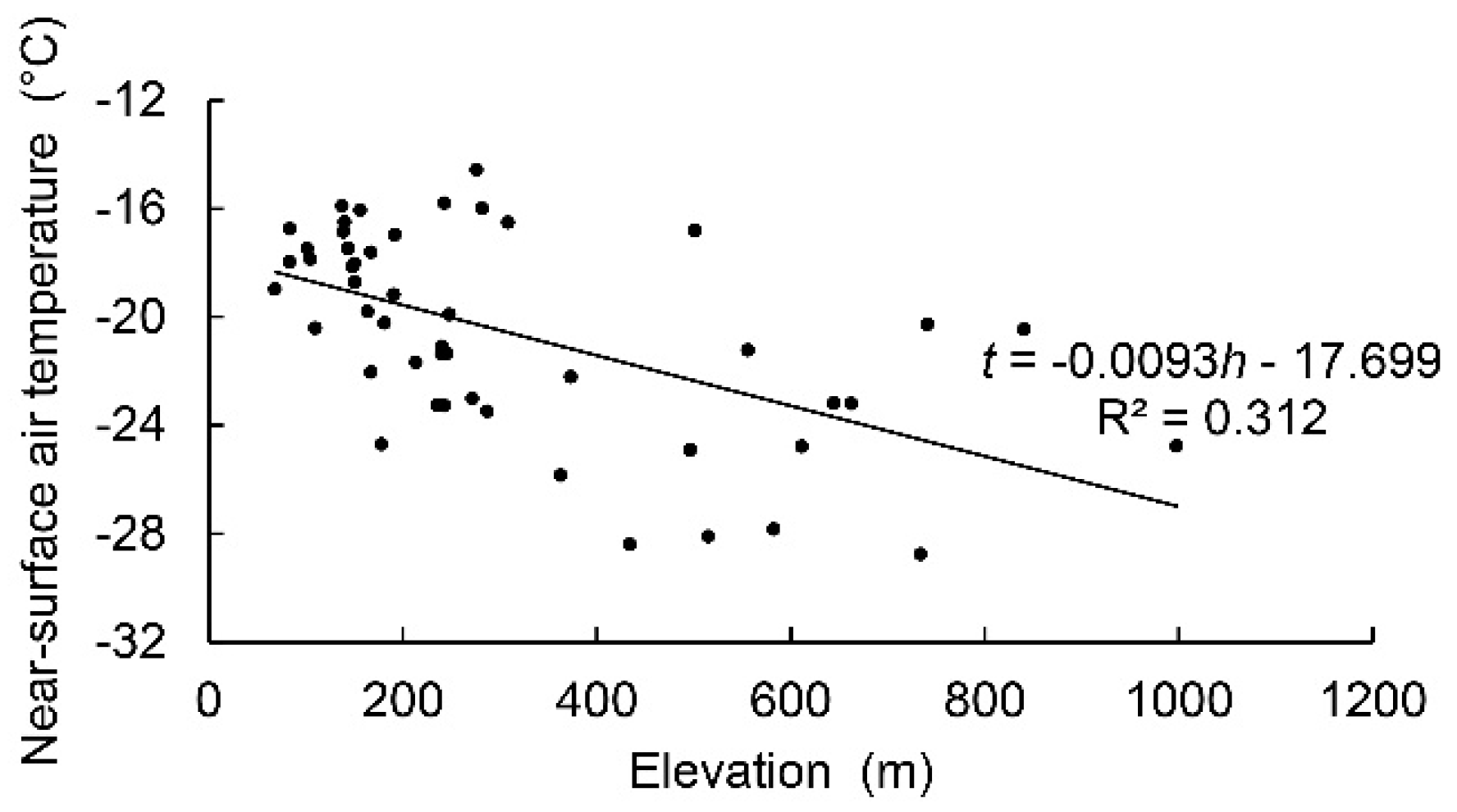
4.3. The Relationship of TLR with Elevation and LST

As a whole, the annual average LST decreased with the increase in elevation (Figure 9a). Steep annual average TLR ( Γ 7 °C/km) occurred frequently at elevations of h > 1.5 km, especially at h > 4 km. In contrast, temperature vertical gradient inversion occurred frequently at h < 1.5 km. The annual average TLR also showed less variability (average standard deviation σ = 2.8 ± 0.1 °C/km at 95% significant level) at 1.5 < h < 4 km than those at other elevations ( σ = 3.7 ± 0.1 °C/km) (Figure 9b).
The monthly average LST also showed a remarkable decreasing trend with elevation in warm months (summer, later spring, and early autumn) (Figure 10). However, as the LST at low altitude could reach the same low as at high altitude in cold months (winter, early spring, and later autumn), the relationship between elevation and LST was complex, especially at h < 2 km. The TLR at h > 5 km was steeper than that at low altitude, in all months. Temperature vertical gradient inversion mostly happened in winter, in cases of low LST and low altitude (h < 2 km), and also in some grids at middle altitude (2 < h < 4 km). The former was represented by Northeast China, and the latter shown by Northwest China. Interestingly, the monthly average TLR was often steeper at higher LST than at low LST, at 2 < h < 6 km, in summer.

4.4. Seasonal Pattern and Magnitude of Variability

The summer pattern, or the patches with the steepest TLR in summer, was widely distributed across most of China; the spring pattern and winter pattern mainly happened in the eastern parts of the Tibetan Plateau, and the autumn pattern mainly took place in the North China Plain (Figure 11a). As the areas with extremely large magnitudes of variability are well matched with the areas of plains and basins with a small terrain slope and a low confidence of the calculating results, focus was given to the rest of the areas. What was different from the previous analyses [22,38,40] was that not all parts of the Tibetan Plateau showed a distinct seasonal pattern, but the eastern region of the plateau did exhibit a winter and spring pattern. Moreover, the winter pattern was mainly distributed in the northern slopes of the Eastern Himalayan Mountains. The smallest magnitude of variability occurred in Central and Southwest China, especially in the Ta-pa Mountains and the Qinling Mountains, and the large magnitude of variability was mostly distributed in the hills and mountainous areas of Northeast China (Figure 11b), where the magnitude of variability could reach more than 15 °C/km.

5. Discussion

LST is an important parameter in the study of the physical processes of land surface. The land-surface TLR could reflect the spatiotemporal variation of thermal processes and the difference of the regional climate. The traditional ways to calculate surface TLR and identify the seasonal pattern are linear regression and line charts, respectively. However, strong spatial heterogeneity led to a large uncertainty, in the TLR estimated through linear regression, for a large region. Generally, stations or grids were divided into several groups and the TLR in each group was calculated separately when the study area was large. Although grouping could improve the accuracy to a certain extent, the grouping results would directly affect the value of the TLR, and sparse meteorological stations in high altitude would result in statistical bias. Meanwhile, as the station grouping was uncertain, different seasonal patterns among small regions could not be distinguished clearly.
Therefore, a methodology was developed in this paper that was composed of a formula which was derived on the basis of the analysis of the temperature field and the height field, an image enhancement technique which was used to calculate the gradient, and FCM clustering which was applied to identify the seasonal pattern of the TLR. Furthermore, the spatiotemporal variation of land-surface TLR in China was analyzed by applying this methodology. The analysis results were broadly in accordance with previous studies. The spatial variability in winter was larger than in summer, which has also been found in previous studies [24,53]. Previous analysis results also showed that the summer pattern is a dominant mode [21,27,33,35,54], which was consistent with the result of this work.
Nevertheless, some previous studies have found that the Tibetan Plateau had a different seasonal pattern when compared to other regions in the world, with the TLR steeper in winter than in summer [22,38,40]. Unlike the previous analyses, however, not all parts of the Tibetan Plateau showed such a distinct seasonal pattern, and this only occurred in the eastern region of the plateau (Figure 11a). Moreover, the TLR of the Eastern Tibetan Plateau was steep, not only in winter, but also in spring, and the winter pattern was mainly distributed in the northern slopes of the Eastern Himalayan Mountains. A major reason for the difference of this analysis from previous ones could be related to the uneven distribution of meteorological stations in the plateau. There are few meteorological stations in the Western Tibetan Plateau (Figure 6a), and the seasonal pattern of TLR, which has been based on linear regressions and meteorological observational data, in previous studies, actually represented only the eastern region. As seasonal pattern could usually be identified by checking the trend of the line chart, which strongly depended on the results of the station grouping, detailed seasonal features based on the small scope have not been researched in the Eastern Tibetan Plateau. Kattel et al. [11] found that the TLR in the northern slopes of the eastern Himalayan Mountains was steep in winter and shallow in summer, which was consistent with our results.
The distinctive seasonal pattern of the TLR in the Eastern Tibetan Plateau was due to the unique climatic regimes, dry and cold in winter, and moist and warm in summer [22]. On one hand, the intense latent heat released at the upper atmosphere (water vapor condensation from moist convection of southwest currents from the Bay of Bengal) and decreasing sensible heat at the surface (heavier rainfall and denser cloudiness) produced the shallowest TLRs in summer in this region; on the other hand, strong sunshine and the resulting sensible heat at the surface in the non-monsoon seasons (November to April) produced the steepest TLR, in winter or spring [37].
As for the Xinjiang Autonomous Region located in Northwest China, temperature vertical gradient inversion has also been observed, in winter, in previous studies [34,38,53]. In Northeast China, however, the results of our analysis were different from some of the previous studies [38,40], which did not observe the phenomenon of temperature vertical gradient inversion, but found a steep TLR in winter. In order to reproduce their results as much as possible, the dataset from the National Meteorological Information Center, China Meteorological Administration (CMA), was used to conduct the linear regression. As shown in Figure 12, a steep monthly average TLR (−9.3 °C/km) was indeed found in the northeastern parts of China (mostly in the northern part of Northeast China). However, though the linear regression was significant, the goodness of fit was low ( R 2 = 0 . 312 ). More than 70% of these stations were located in low altitude (<400 m), which accounted for less than 50% of the explained sum of squares (ESS), and most residuals through linear regression came from those in high altitude.
The meteorological stations were mostly distributed in and around the Northeast Plain with low altitude (not shown), but there were a few in the Greater Khingan Mountains and Lesser Khingan Mountains, at higher altitudes. As there were only a few stations in the mountainous and the hilly areas, the temperature vertical gradient inversion could not be seen clearly. The magnitude of variability of the TLR could reach more than 15 °C/km, in Northeast China (Figure 11b), which revealed a greatly different TLR, within a year. There was a temperature vertical gradient inversion in the Lesser Khingan Mountains and in the western and northern parts of the Greater Khingan Mountains, in winter and early spring, but a steep TLR in some places of the Eastern Greater Khingan Mountains was also notable (Figure 4). The temperature vertical gradient inversion, in the Greater Khingan Mountains and Lesser Khingan Mountains, has also been reported in some other previous studies [55,56].
The widely distributed temperature vertical gradient inversion in the Northeast, Northwest, and North China, in winter, may be related to the complex topography, including the cold air lake effect, in the cold months, in the basins and lowlands of the northern parts of China [57,58]. It is also interesting to note that the temperature vertical gradient inversion was distributed in the western and northern parts of the Greater Khingan Mountains, in winter and in early spring, while a steep TLR has been found in the eastern parts of the mountains. The former may be related to a persistent snow cover, while the latter might have been caused by the unique Foehn effect, during these seasons. On one hand, persistent snow cover and the inherent geomorphology might have been the main factors for the formation of temperature vertical gradient inversion. The winter snow cover in the mountains and plateau caused strong cooling near the surface and an obvious temperature vertical gradient inversion; the plateau west of the Greater Khingan Mountains acted as a quasi-basin where cold air masses from the northwest were more easily kept, at the surface, benefiting the formation and development of the temperature vertical gradient inversion. On the other hand, as the Greater Khingan Mountains are located west of the Northeast Plain, when the northwest wind passed by in winter, the relatively warm air currents above the cool air masses in the Western and Northern Greater Khingan Mountains descended along the leeward slopes, which led to a steep TLR in the eastern parts of the mountains [59].
In addition, the smallest magnitude of variability occurred in the Central and Southwest China, especially in the Ta-pa Mountains and the Qinling Mountains. This was due to the relatively large cloudiness and rainfall in the subtropical monsoon climate, which is characterized by not so high temperature in summer and not so cold temperature in winter, as the cold currents of the northwest winds are blocked away from the southern slopes of the Qinling Mountains. Hence, the small intra-seasonal variability of temperature produced a relatively stable TLR.
The TLR at very high altitudes (>5 km) was steeper than at low altitudes, in all months. It was also found that the TLR generally increased with altitude [28]. This might be the result of low air humidity at high altitude. As water vapor holds larger latent heat than dry air, when air with little vapor arises, the temperature decreases quickly. Meanwhile, compared with high altitude, the temperature vertical gradient inversion was more likely to happen in low altitude, in winter.
With the prevalence of satellite remote-sensing technology, the development of the methodology for calculating and analyzing TLR, based on the grid data, is necessary, therefore, especially for the studies of TLR in a large region with a complex topography. In this research, a formula derived on the basis of the analysis of the temperature field and the height field could provide a new procedure to calculate and analyze the TLR, which is beneficial to the study of mountainous microclimates. Moreover, an image enhancement technique was used for the calculation of TLR and the FCM clustering method was applied to the identification of seasonal patterns, the combination of which made it possible to analyze the TLR, on a large spatial scale. In addition, as the methodology was based on grid data, it was also applicable for estimating and analyzing the near-surface air TLR of a large region when the datasets had been transformed into grid data, and further in the studies of mountainous climate and regional climate change.
As LST is related to land use and vegetation cover, which might change with anthropogenic influences [60,61], the gradient of the LST might also change, correspondingly. Depending on the gradient of the LST, the land-surface TLR becomes changeable, especially in regions with denser populations. These changes might increase the spatial heterogeneity of land-surface TLR, which would increase the noises of land-surface TLR images and reduce the accuracy of the methodology. Considering this deficiency, stratifying the results with land use maps or vegetation index data might be another promising way to analyze the variation of the land-surface TLR and to find the relationship between the land-surface TLR and land cover.

6. Conclusions

A new methodology was developed in this paper to calculate and analyze the land-surface TLR. With this methodology, the spatial and temporal pattern of the TLR in China was analyzed, and some new findings were reported and discussed.
Surface temperature vertical gradient inversion widely occurred in Northeast, Northwest, and North China, in winter, especially in the Xinjiang Autonomous Region, northern and western parts of the Greater Khingan Mountains, the Lesser Khingan Mountains, and the northern area of Northwest and North China. The summer pattern, which was characterized by the steepest TLR during summertime, was distributed more widely throughout China. The Eastern Tibetan Plateau held a distinct seasonal pattern, when compared to other regions in the world, with a steep TLR in winter and spring, and a shallow TLR in summer. The temperature vertical gradient inversion phenomenon occurred widely in Northeast China, in winter and early spring, with a strong temperature vertical gradient inversion in western and northern parts of the Greater Khingan Mountains, but a steep TLR appeared in some parts of the eastern slopes of the mountains. A large magnitude of variability of TLR was found in Northeast China, where there was a steep TLR in spring and summer, and a strong temperature vertical gradient inversion in winter. The smallest magnitude of variability occurred in Central and Southwest China, especially in the Ta-pa Mountains and the Qinling Mountains. The TLR at high altitude was generally steeper than at low altitude, and was usually steeper at very high altitude (>5 km) than at low altitude, in all months of the year.
The methodology developed in this study has the potential to be applied for estimating grid near-surface air TLR of a large region with complex topographical and geographical conditions, and further in the studies of mountainous climates and regional climate change, in the future. However, as only one case was used for the application of this methodology in this paper, the choice of the spatial resolution was not discussed. Furthermore, the treatment of the near-zero gradient of height was somehow rough. These two issues of the methodology, developed in this article, should be improved in future studies. The spatial resolution can be adjusted to meet the different needs of studies in diverse spatial scales. In order to shrink the influence of noise and obtain detailed information on TLR, as much as possible, high-resolution data are suggested for the study of a smaller region. Mid-low resolution data are suitable for the study of a larger region. In consideration of the relationship between the LST and the land-use and vegetation cover, it would be a promising procedure to analyze the land-surface TLR, by stratifying the results with the land-use maps or vegetation index data.

Author Contributions

Y.Q. developed the methodology, performed the calculations, and wrote the manuscript. G.R. conducted the study, contributed to the interpretation of the results, and reviewed the manuscript. T.Z. provided technical support, made the geographical divisions, and reviewed the manuscript. P.Z. and K.W. validated and reviewed the manuscript.

Funding

This work was supported by the Chinese Ministry of Science and Technology (MOST) National Key R&D Program (No. 2018YFA0605603) and the Natural Science Foundation of China (NSFC) (No. 41575003).

Acknowledgments

We thank two anonymous reviewers for providing constructive comments, which greatly improved this manuscript.

Conflicts of Interest

The authors declare no conflict of interest.

References

  1. Noilhan, J.; Planton, S. A simple parameterization of land surface processes for meteorological models. Mon. Weather Rev. 1989, 117, 536–549. [Google Scholar] [CrossRef]
  2. Wang, L.; Sun, L.; Shrestha, M.; Li, X.; Liu, W.; Zhou, J.; Yang, K.; Lu, H.; Chen, D. Improving snow process modeling with satellite-based estimation of near-surface-air-temperature lapse rate. J. Geophys. Res. Atmos. 2016, 12, 5–30. [Google Scholar] [CrossRef]
  3. Wan, Z.; Wang, P.; Li, X. Using MODIS land surface temperature and normalized difference vegetation index products for monitoring drought in the southern Great Plains, USA. Int. J. Remote Sens. 2004, 25, 61–72. [Google Scholar] [CrossRef]
  4. Sow, M.; Mbow, C.; Hély, C.; Fensholt, R.; Sambou, B. Estimation of herbaceous fuel moisture content using vegetation indices and land surface temperature from MODIS data. Remote Sens. 2013, 5, 2617–2638. [Google Scholar] [CrossRef]
  5. Zhang, D.; Tang, R.; Zhao, W.; Tang, B.; Wu, H.; Shao, K.; Li, Z. Surface soil water content estimation from themal remote sensing based on the temporal variation of land surface temperature. Remote Sens. 2014, 6, 3170–3187. [Google Scholar] [CrossRef] [Green Version]
  6. Clinton, N.; Gong, P. MODIS detected surface urban heat islands and sinks: Global locations and controls. Remote Sens. Environ. 2013, 134, 294–304. [Google Scholar] [CrossRef]
  7. Schwarz, N.; Lautenbach, S.; Seppelt, R. Exploring indicators for quantifying surface urban heat islands of European cities with MODIS land surface temperatures. Remote Sens. Environ. 2011, 115, 3175–3186. [Google Scholar] [CrossRef]
  8. Tomlinson, C.J.; Chapman, L.; Thornes, J.E.; Baker, C.J. Derivation of Birmingham’s summer surface urban heat island from MODIS satellite images. Int. J. Climatol. 2012, 32, 214–224. [Google Scholar] [CrossRef]
  9. Justice, C.O.; Townshend, J.R.G.; Vermote, E.F.; Masuoka, E.; Wolfe, R.E.; Saleous, N.; Roy, D.P.; Morisette, J.T. An overview of MODIS land data processing and product status. Remote Sens. Environ. 2002, 83, 3–15. [Google Scholar] [CrossRef]
  10. Tang, C.Q. Forest vegetation as related to climate and soil conditions at varying altitudes on a humid subtropical mountain, Mount Emei, Sichuan, China. Ecol. Res. 2006, 21, 174–180. [Google Scholar] [CrossRef]
  11. Kattel, D.B.; Yao, T.; Yang, W.; Gao, Y.; Tian, L. Comparison of temperature lapse rates from the northern to the southern slopes of the Himalayas. Int. J. Climatol. 2015, 35, 4431–4443. [Google Scholar] [CrossRef]
  12. Mountain Research Initiative EDW Working Group. Elevation-dependent warming in mountain regions of the world. Nat. Clim. Chang. 2015, 5, 424–430. [Google Scholar] [CrossRef] [Green Version]
  13. Zhu, W.; Lü, A.; Jia, S. Estimation of daily maximum and minimum air temperature using MODIS land surface temperature products. Remote Sens. Environ. 2013, 130, 62–73. [Google Scholar] [CrossRef]
  14. Neteler, M. Estimating daily land surface temperatures in mountainous environments by reconstructed MODIS LST data. Remote Sens. 2010, 2, 333–351. [Google Scholar] [CrossRef]
  15. Williamson, S.N.; Hik, D.S.; Gamon, J.A.; Kavanaugh, J.L.; Flowers, G.E. Estimating temperature fields from MODIS land surface temperature and air temperature observations in a sub-Arctic Alpine environment. Remote Sens. 2014, 6, 946–963. [Google Scholar] [CrossRef]
  16. Benali, A.; Carvalho, A.C.; Nunes, J.P.; Carvalhais, N.; Santos, A. Estimating air surface temperature in Portugal using MODIS LST data. Remote Sens. Environ. 2012, 124, 108–121. [Google Scholar] [CrossRef]
  17. Zhang, H.; Zhang, F.; Zhang, G.; Che, T.; Yan, W. How accurately can the air temperature lapse rate over the Tibetan Plateau be estimated from MODIS LSTs? J. Geophys. Res. Atmos. 2018, 123, 3943–3960. [Google Scholar] [CrossRef]
  18. Jin, M.; Dickinson, R.E. Land surface skin temperature climatology: Benefitting from the strengths of satellite observations. Environ. Res. Lett. 2010, 5, 044004. [Google Scholar] [CrossRef]
  19. Good, E.J.; Ghent, D.J.; Bulgin, C.E.; Remedios, J.J. A spatiotemporal analysis of the relationship between near-surface air temperature and satellite land surface temperatures using 17 years of data from the ATSR series. J. Geophys. Res. Atmos. 2017, 122, 9185–9210. [Google Scholar] [CrossRef]
  20. Wang, Y.; Wang, L.; Li, X.; Chen, D. Temporal and spatial changes in estimated near-surface air temperature lapse rates on Tibetan Plateau. Int. J. Climatol. 2018, D24, 1–15. [Google Scholar] [CrossRef]
  21. Rolland, C. Spatial and seasonal variations of air temperature lapse rates in Alpine Regions. J. Clim. 2003, 16, 1032–1046. [Google Scholar] [CrossRef]
  22. Guo, X.; Wang, L.; Tian, L. Spatio-temporal variability of vertical gradients of major meteorological observations around the Tibetan Plateau. Int. J. Climatol. 2016, 36, 1901–1916. [Google Scholar] [CrossRef]
  23. Chiu, C.A.; Lin, P.H.; Tsai, C.Y. Spatio-temporal variation and monsoon effect on the temperature lapse rate of a subtropical island. Terr. Atmos. Ocean. Sci. 2014, 25, 203–217. [Google Scholar] [CrossRef]
  24. Blandford, T.R.; Humes, K.S.; Harshburger, B.J.; Moore, B.C.; Walden, V.P.; Ye, H. Seasonal and synoptic variations in near-surface air temperature lapse rates in a mountainous basin. Theor. Appl. Climatol. 2008, 47, 249–261. [Google Scholar] [CrossRef]
  25. Hartmann, D.L. Global Physical Climatology, 2nd ed.; Elsevier: Waltham, MA, USA, 2016; ISBN 9780123285317. [Google Scholar]
  26. Harlow, R.C.; Burke, E.J.; Scott, R.L.; Shuttleworth, W.J.; Brown, C.M.; Petti, J.R. Research note: Derivation of temperature lapse rates in semi-arid south-eastern Arizona. Hydrol. Earth Syst. Sci. 2004, 8, 1179–1185. [Google Scholar] [CrossRef]
  27. Marshall, S.J.; Sharp, M.J.; Burgess, D.O.; Anslow, F.S. Near-surface-temperature lapse rates on the Prince of Wales Icefield, Ellesmere Island, Canada: Implications for regional downscaling of temperature. Int. J. Climatol. 2007, 27, 385–398. [Google Scholar] [CrossRef]
  28. Pepin, N.; Losleben, M. Climate change in the Colorado Rocky Mountains: Free air versus surface temperature trends. Int. J. Climatol. 2002, 22, 311–329. [Google Scholar] [CrossRef]
  29. Mokhov, I.I.; Akperov, M.G. Tropospheric lapse rate and its relation to surface temperature from reanalysis data. Izv. Atmos. Ocean. Phys. 2006, 42, 430–438. [Google Scholar] [CrossRef]
  30. Whiteman, C.D. Mountain Meteorology Fundamentals and Applications; Oxford University Press: New York, NY, USA, 2000; ISBN 0195132718. [Google Scholar]
  31. Whiteman, C.D.; Bian, X.; Zhong, S. Wintertime evolution of the temperature inversion in the Colorado Plateau Basin. J. Appl. Meteorol. 1999, 38, 1103–1117. [Google Scholar] [CrossRef]
  32. Kirchner, M.; Faus-Kessler, T.; Jakobi, G.; Leuchner, M.; Ries, L.; Scheel, H.E.; Suppan, P. Altitudinal temperature lapse rates in an Alpine valley: Trends and the influence of season and weather patterns. Int. J. Climatol. 2013, 33, 539–555. [Google Scholar] [CrossRef]
  33. Tang, Z.; Fang, J. Temperature variation along the northern and southern slopes of Mt. Taibai, China. Agric. For. Meteorol. 2006, 139, 200–207. [Google Scholar] [CrossRef]
  34. Du, M.; Zhang, M.; Wang, S.; Zhu, X.; Che, Y. Near-surface air temperature lapse rates in Xinjiang, northwestern China. Theor. Appl. Climatol. 2018, 131, 1221–1234. [Google Scholar] [CrossRef]
  35. Minder, J.R.; Philip, W.M.; Lundquist, J.D. Surface temperature lapse rates over complex terrain: Lessons from the Cascade Mountains. J. Geophys. Res. 2010, 115, D14122. [Google Scholar] [CrossRef]
  36. Pepin, N.; Kidd, D. Spatial temperature variation in the Eastern Pyrenees. Weather 2006, 61, 300–310. [Google Scholar] [CrossRef]
  37. Kattel, D.B.; Yao, T.; Panday, P.K. Near-surface air temperature lapse rate in a humid mountainous terrain on the southern slopes of the eastern Himalayas. Theor. Appl. Climatol. 2018, 132, 1129–1141. [Google Scholar] [CrossRef]
  38. Li, X.; Wang, L.; Chen, D.; Yang, K.; Xue, B.; Sun, L. Near-surface air temperature lapse rates in the mainland China during 1962–2011. J. Geophys. Res. Atmos. 2013, 118, 7505–7515. [Google Scholar] [CrossRef]
  39. Dodson, R.; Marks, D. Daily air temperature interpolated at high spatial resolution over a large mountainous region. Clim. Res. 1997, 8, 1–20. [Google Scholar] [CrossRef] [Green Version]
  40. Li, Y.; Zeng, Z.; Zhao, L.; Piao, S. Spatial patterns of climatological temperature lapse rate in mainland China: A multi–time scale investigation. J. Geophys. Res. Atmos. 2015, 120, 2661–2675. [Google Scholar] [CrossRef]
  41. Jain, S.K.; Goswami, A.; Saraf, A.K. Determination of land surface temperature and its lapse rate in the Satluj River basin using NOAA data. Int. J. Remote Sens. 2008, 29, 3091–3103. [Google Scholar] [CrossRef]
  42. Liu, Y.; Li, F. A Preliminary Approach on the Land Surface Temperature (LST) Lapse Rate of Mountain Area Using MODIS Data; Remote Sensing and Space Technology for Multidisciplinary Research and Applications, International Society for Optics and Photonics: Beijing, China, 2006; Volume 619907. [Google Scholar]
  43. Fischer, M.M.; Getis, A. Handbook of Applied Spatial Analysis: Software Tools, Methods and Applications; Springer: New York, NY, USA, 2010; ISBN 9783642036460. [Google Scholar]
  44. Dubrovin, B.A.; Fomenko, A.T.; Novikov, S.P. Modern Geometry-Methods and Applications, Part I, The Geometry of Surfaces, Transformation Groups, and Fields, 2nd ed.; Springer: New York, NY, USA, 1992; ISBN 0387976639. [Google Scholar]
  45. Schey, H.M. Div, Grad, Curl, and All That: An Informal Text on Vector Calculus, 4th ed.; W.W. Norton & Company, Inc.: New York, NY, USA, 2005; ISBN 0393925161. [Google Scholar]
  46. Korn, G.A.; Korn, T.M. Mathematical Handbook for Scientists and Engineers: Definitions, Theorems, and Formulas for Reference and Review; Mc. Graw. Dover: New York, NY, USA, 1961; ISBN 0486411478. [Google Scholar]
  47. Solomon, C.J.; Breckon, T.P. Fundamentals of Digital Image Processing: A Practical Approach with Examples in Matlab; Wiley Blackwell: New York, NY, USA, 2011; ISBN 0470844728. [Google Scholar]
  48. Gonzalez, R.C.; Woods, R.E.; Eddins, S.L. Digital Image Processing Using Matlab, 2nd ed.; Gatesmark Publishing: Knoxville, TN, USA, 2009; ISBN 9780982085400. [Google Scholar]
  49. Bezdek, J.C. Pattern Recognition with Fuzzy Objective Function Algorithms; Springer: New York, NY, USA; 1981; ISBN 1475704526. [Google Scholar]
  50. Snyder, J.P. Flattening the Earth: Two Thousand Years of Map Projections; The University of Chicago Press: Chicago, IL, USA, 1997; ISBN 0226767477. [Google Scholar]
  51. Sobel, I. History and Definition of the Sobel Operator. 2014. Available online: https://www.researchgate.net/publication/239398674_An_Isotropic_3_3_Image_Gradient_Operator (accessed on 14 June 2015).
  52. Nixon, M.S.; Aguado, A.S. Feature Extraction and Image Processing, 3rd ed.; Academic Press: London, UK, 2012; ISBN 0123965497. [Google Scholar]
  53. Shen, Y.-J.; Shen, Y.; Goetz, J.; Brenning, A. Spatial-temporal variation of near-surface temperature lapse rates over the Tianshan Mountains, central Asia. J. Geophys. Res. Atmos. 2016, 121, 14006–14017. [Google Scholar] [CrossRef]
  54. Gardner, A.S.; Sharp, M.J.; Koerner, R.M.; Labine, C.; Boon, S.; Marshall, S.J.; Burgess, D.O.; Lewis, D. Near-surface temperature lapse rates over Arctic Glaciers and their implications for temperature downscaling. J. Clim. 2009, 22, 4281–4298. [Google Scholar] [CrossRef]
  55. Zhao, J.; Lu, Z.; Meng, Y. Influence of the temperature inversion to the weather in Daxinganling Region. J. Anhui Agric. Sci. 2014, 42, 6741–6756. (In Chinese) [Google Scholar]
  56. Lollino, G.; Manconi, A.; Clague, J.; Shan, W.; Chiarle, M. Engineering Geology for Society and Territory—Volume 1: Climate Change and Engineering Geology; Springer: New York, NY, USA, 2015; pp. 271–277, 285–290. ISBN 9783319092997. [Google Scholar]
  57. Petkovšek, Z. Turbulent dissipation of cold air lake in a basin. Meteorol. Atmos. Phys. 1992, 47, 237–245. [Google Scholar] [CrossRef]
  58. Zhong, S.; Whiteman, C.D.; Bian, X.; Shaw, W.J.; Hubbe, J.M. Meteorological processes affecting the evolution of a wintertime cold air pool in the Columbia Basin. Mon. Weather Rev. 2001, 129, 2600–2613. [Google Scholar] [CrossRef]
  59. Weng, D.; Sun, Z. A preliminary study of the lapse rate of surface air temperature over mountainous regions of China. Geogr. Res. 1984, 3, 24–34. (In Chinese) [Google Scholar]
  60. Amiri, R.; Weng, Q.; Alimohammadi, A.; Alavipanah, S.K. Spatial-temporal dynamics of land surface temperature in relation to fractional vegetation cover and land use/cover in the Tabriz urban area, Iran. Remote Sens. Environ. 2009, 113, 2606–2617. [Google Scholar] [CrossRef]
  61. Ahmed, B.; Kamruzzaman, M.; Zhu, X.; Rahman, M.S.; Choi, K. Simulating land cover changes and their impacts on land surface temperature in Dhaka, Bangladesh. Remote Sens. 2013, 5, 5969–5998. [Google Scholar] [CrossRef] [Green Version]
Figure 1. Contour of homogeneous height field (dashed line) and temperature field (solid line). Contour lines of the height field and the temperature field are given as h and t , respectively ( h 1 < h 2 < h 3 < h 4 , t 1 < t 2 < t 3 < t 4 < t 5 < t 6 ). The northward and southeastward arrow show the direction of the gradient of height and temperature, respectively. P A , P B , , P E represent the geographical positions on a two-dimensional map. The arc between P B and P D is part of a circle centered on P A .
Remotesensing 10 01617 g001
Figure 2. Topography of the study area (China) and seven geographical divisions.
Remotesensing 10 01617 g002
Figure 3. Spatial distribution of the annual average TLR during 2001–2015. The spatial resolution is 10 km × 10 km. The color bar shows twenty-seven levels of the TLR.
Remotesensing 10 01617 g003
Figure 4. As Figure 3 but of the monthly average TLR. The blue and orange color indicate the image pixels with 15 < Γ 7 and 0 < Γ 10 °C/km, respectively. The white color indicates the other TLR values.
Remotesensing 10 01617 g004
Figure 5. Bar chart of the percentage of image pixels for the steep TLR (blue) and the temperature vertical gradient inversion (red) in each region. The primary and secondary Y-axis represent the percentages for the steep TLR and the temperature vertical gradient inversion, respectively.
Remotesensing 10 01617 g005
Figure 6. The region-wide monthly average TLR of the Tibetan Plateau (a and c) and the Greater Khingan Mountains (b and d). The white circles in the patches (a) and (b) represent the ground meteorological stations. The dividing line in patch (a) indicates east and west of the plateau with much more stations in the east, and patch (b) indicates the mountain ridgeline. The TLR in patches (c) and (d) are the average of the TLR values of image pixels with 15 < Γ 10 °C/km in every month.
Remotesensing 10 01617 g006
Figure 7. Variation of monthly accumulated percentage at each level of the TLR and the country-wide monthly average TLR. The primary Y-axis represents the accumulated percentage of image pixels at each level; the secondary Y-axis represents the country-averaged monthly average TLR. The dashed line is the dividing line between levels of Γ 0 and Γ > 0 °C/km. The solid line is the mean of the monthly average TLR of the image pixels, where 15 < Γ 10 °C/km.
Remotesensing 10 01617 g007
Figure 8. Profile of the monthly average TLR with elevation (a) and LST (b). The color bar shows twenty-five levels of TLR with 15 < Γ 10 °C/km. The spacing of elevation was 50 m (a) and that of LST was 1 °C (b). The value of a grid was the mean of the TLR of the image pixels where the TLRs ranged within the grid bound. If the number of above-mentioned image pixels was less than two, the value was assigned as null
Remotesensing 10 01617 g008
Figure 9. The relationship of the mean (a) and standard deviation (b) of the annual average TLR with elevation and the annual average LST. The spacing of elevation was 50 m and that of LST was 1 °C. The value of a grid in patch a (b) was the mean (standard deviation) of the TLRs of the image pixels, where TLRs ranged within the grid bound. If the number of above-mentioned image pixels was less than two, the value was assigned as null. The slope of the solid line in patch (a) represents a reference TLR of −6.5 °C/km. The color bar in patch (a) is the same as that in Figure 8.
Remotesensing 10 01617 g009
Figure 10. As Figure 9a but of the monthly average TLR with elevation and the monthly average LST. The color bar is the same as that in Figure 9a.
Remotesensing 10 01617 g010
Figure 11. Seasonal pattern (a) and magnitude of variability (b) of the TLR. The type of seasonal pattern in patch (a) indicates in which season the steepest TLR took place. The magnitude of variability in patch (b) represents how much the TLR changed within a year. The grey color indicates the patches where the confidence of the calculating results was low due to the flat topography.
Remotesensing 10 01617 g011
Figure 12. Scatter of elevation and near-surface air temperature in the northeastern parts of China in January, during 1981–2010. Elevation and near-surface air temperature are denoted by h and t in the equation of linear regression, respectively. A total of forty-nine meteorological stations were selected by using the same division standard as Li et al. [38], and the stations were located in the north at 45°N and in the east at 115°E.
Remotesensing 10 01617 g012

