Radiometric Correction of Landsat-8 and Sentinel-2A Scenes Using Drone Imagery in Synergy with Field Spectroradiometry

 , , and
Abstract
:
1. Introduction and Objectives
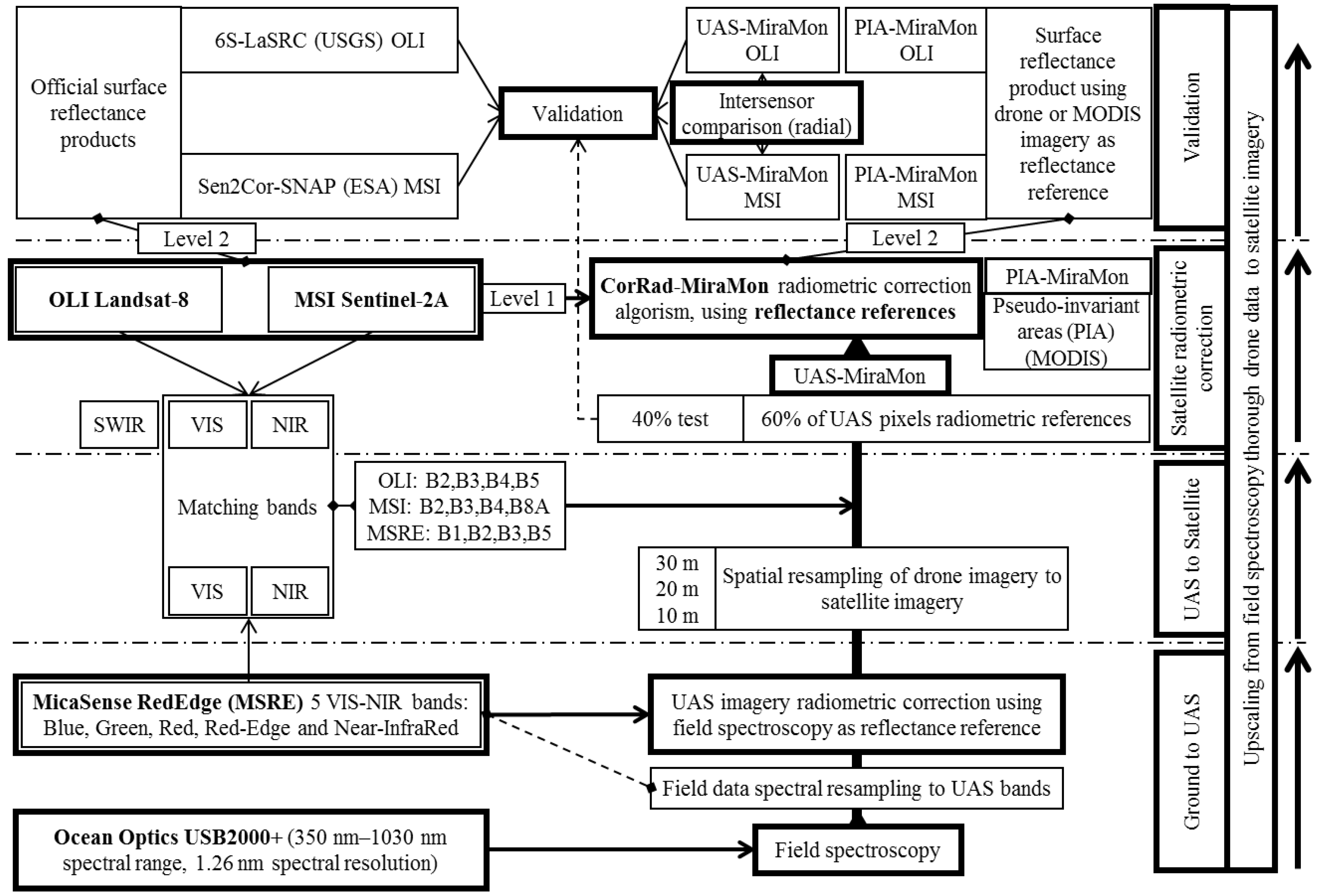
- Radiometrically correcting drone data by using calibration panels and field spectroradiometric measurements;
- Using drone corrected and upscaled data to validate different radiometric products (PIA-MiraMon, 6S-LaSRC and Sen2Cor-SNAP). This point fulfills the second main objective;
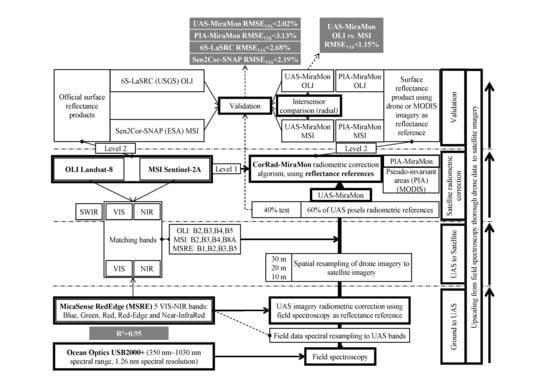
- Splitting the drone corrected and upscaled data into fitting pixels and test pixels. Fitting pixels are used to feed the UAS-MiraMon satellite radiometric correction approach based on field spectroradiometric data in synergy with drone data. Test pixels are used to validate the new method. This point fulfills the first main objective. Additionally, as a second validation we compare the results of UAS-MiraMon with the current 6S-LaSRC, Sen2Cor-SNAP and PIA-MiraMon methods. This complements the second main objective;
- By taking advantage of the almost simultaneous acquisitions of our experimental design, we evaluate the L8 and S2 inter-sensor fitting for the UAS-MiraMon method. This is done at different radial distances from the study area, as we hypothesized that the accuracy of the new UAS-MiraMon method could be better in the drone area. However, we also hypothesized that the accuracy could decrease with increasing distance (local overfitting). This point complements the first main objective.
2. Study Area
3. Materials and Methods
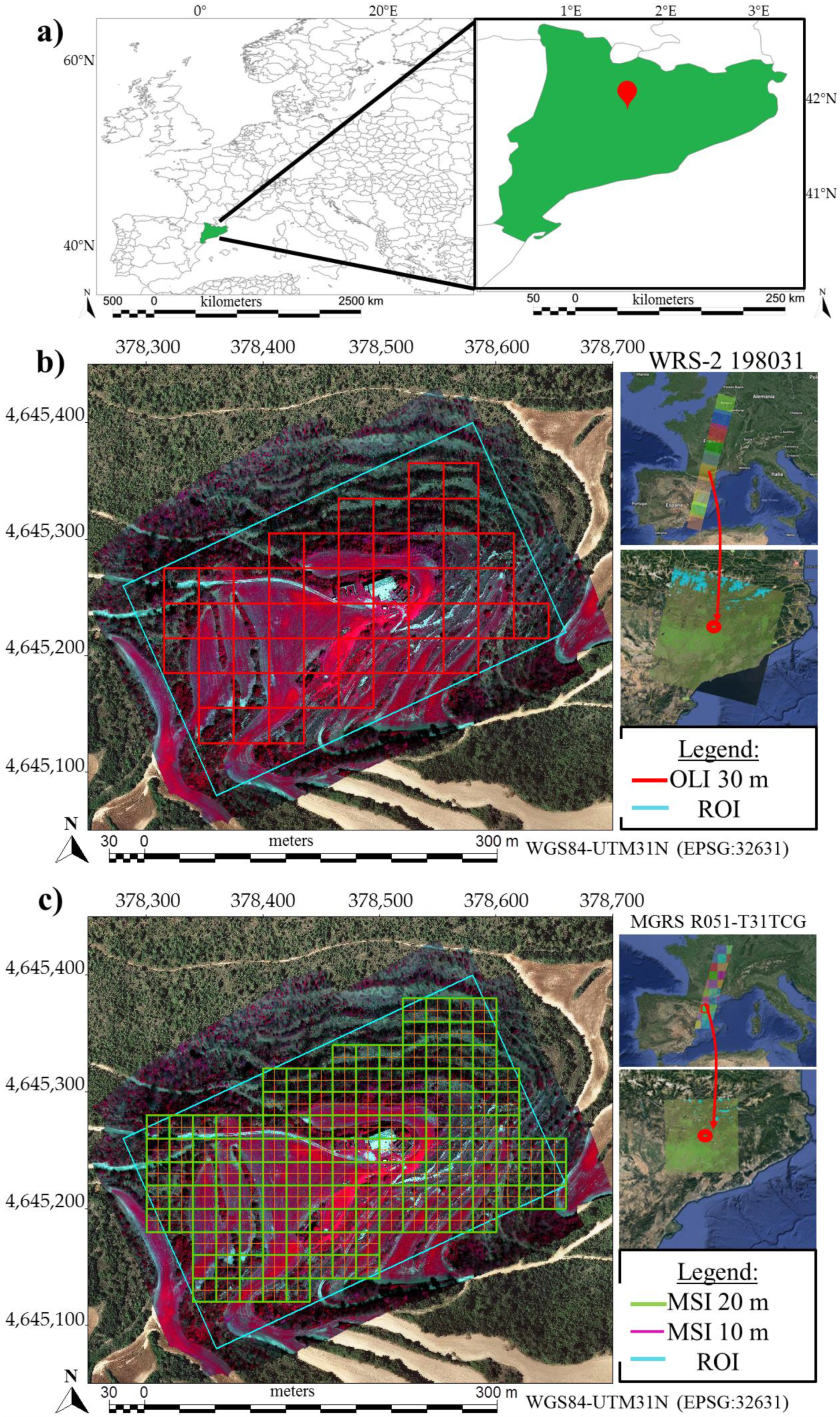
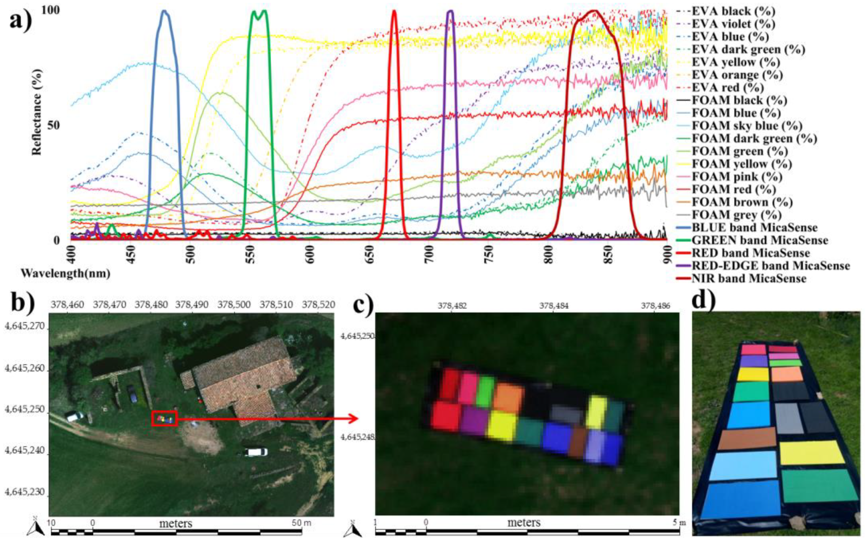
3.1. Field Spectroradiometric Data
3.2. Unmanned Aerial System Data
3.3. Satellite Data
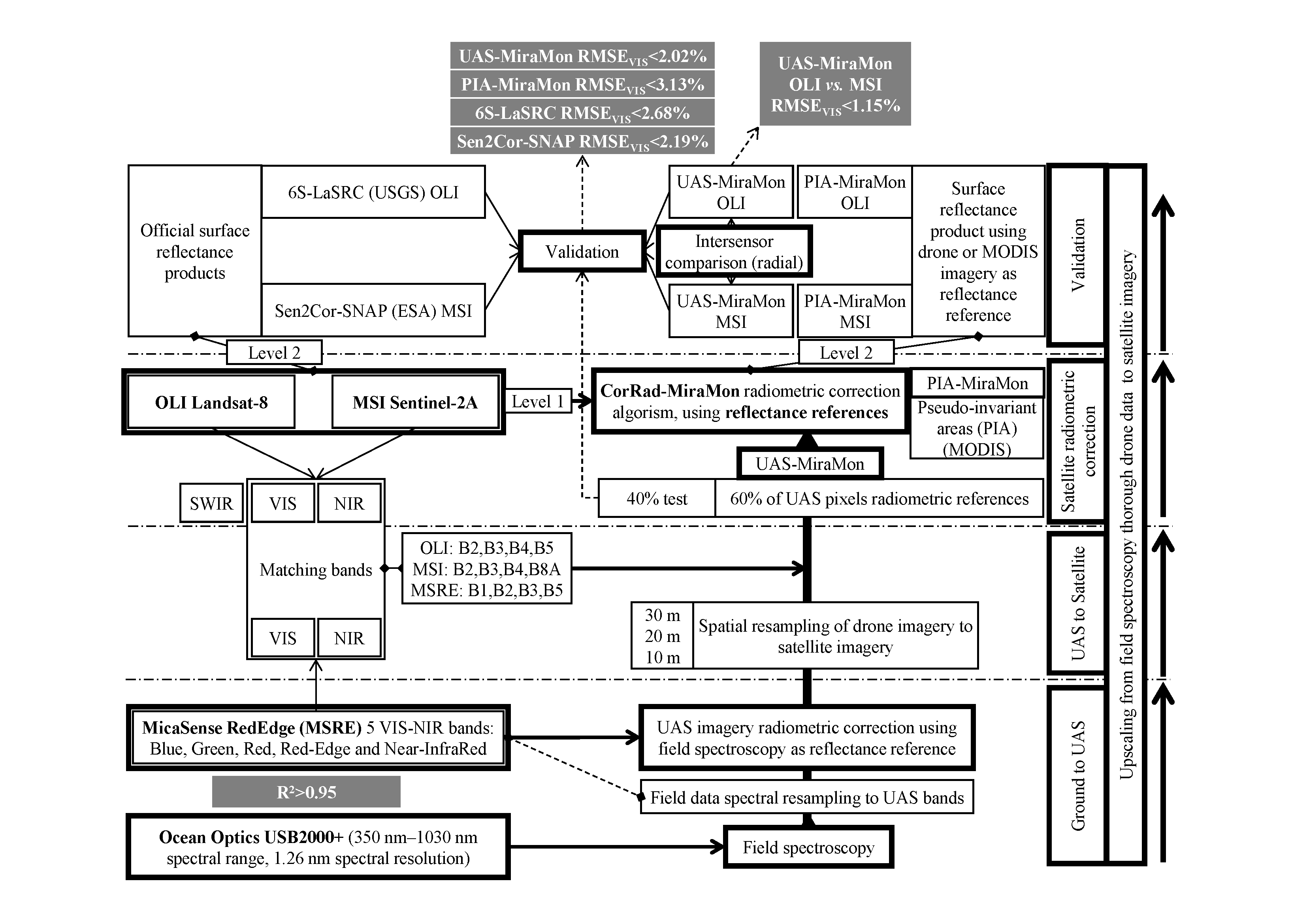
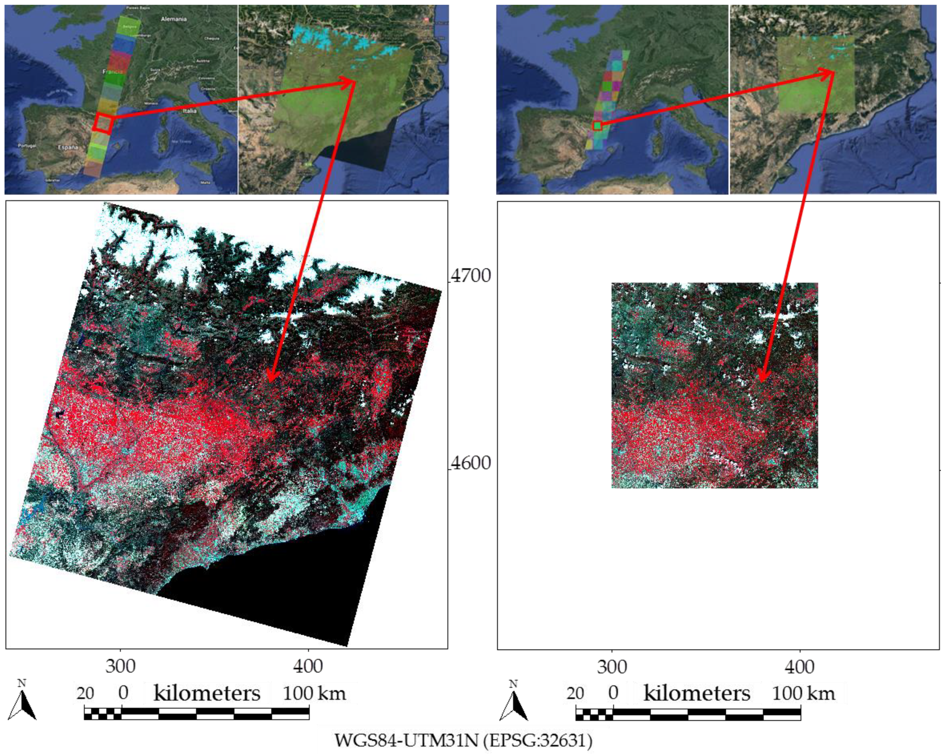
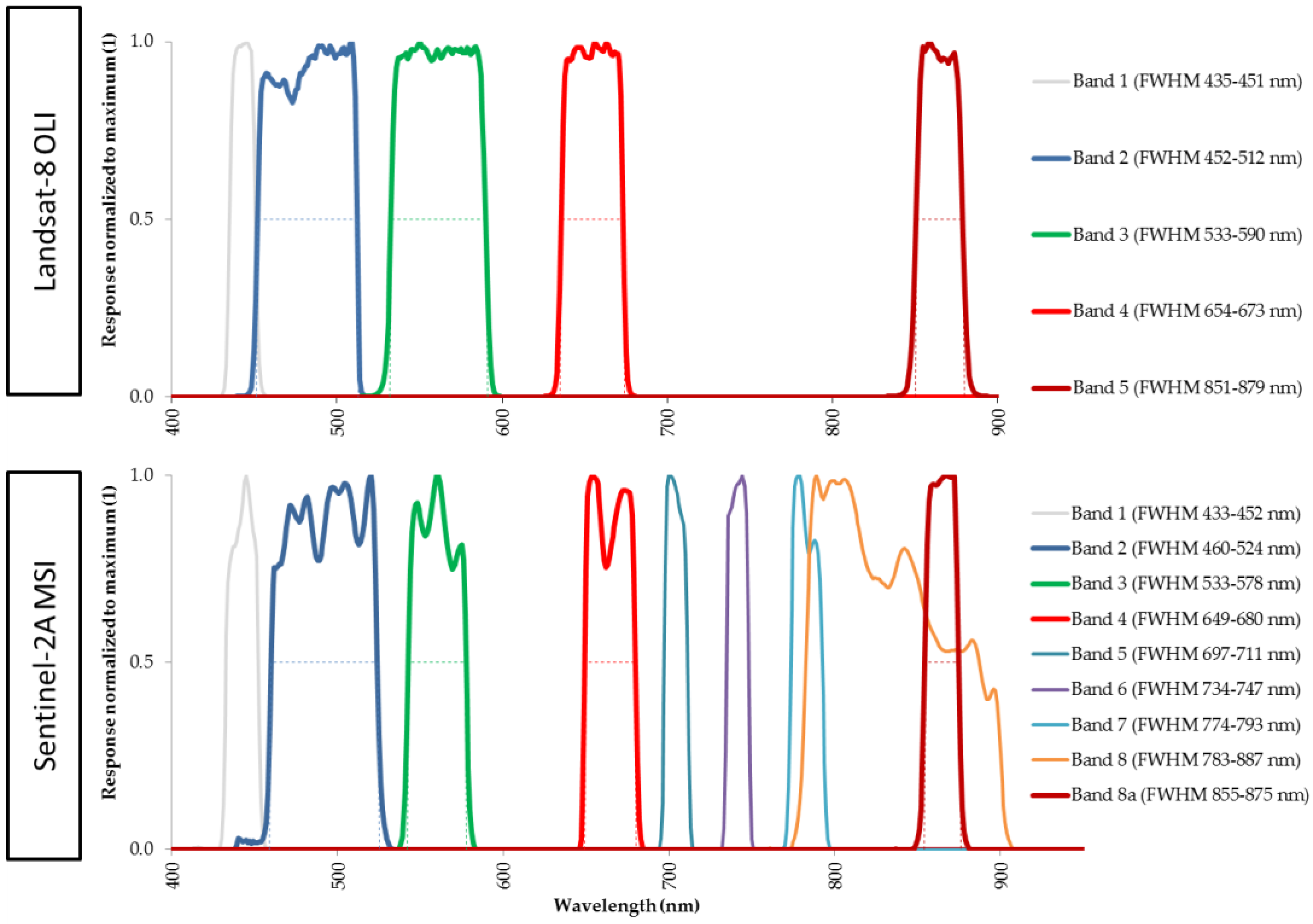
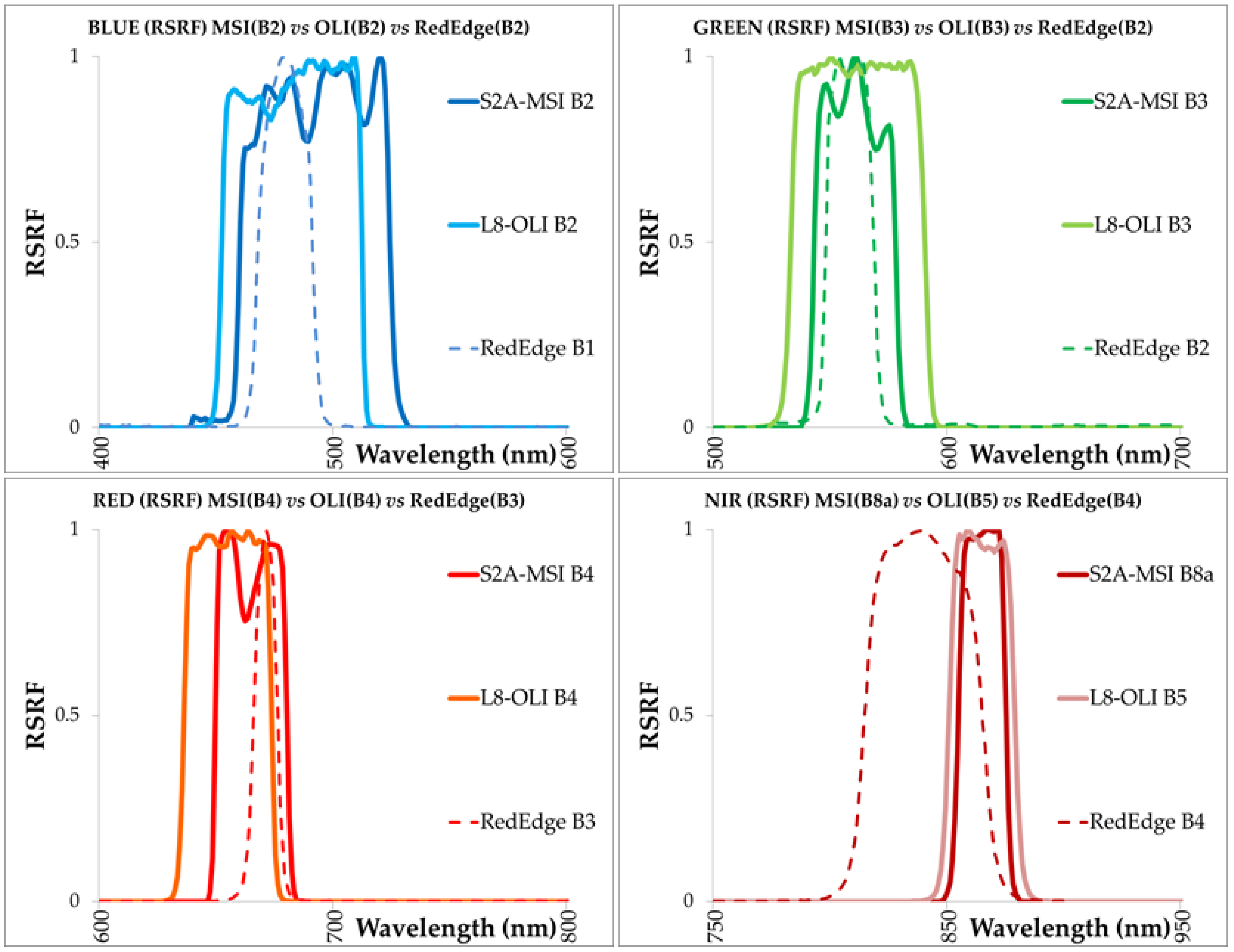
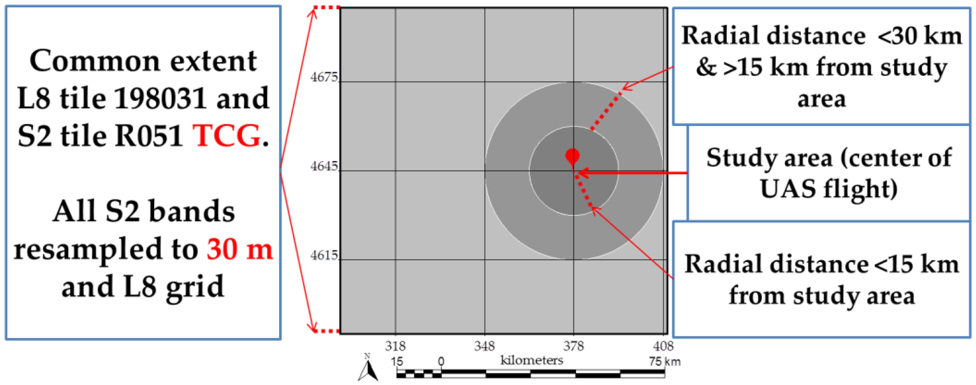
- L8 OLI: The L8 satellite was launched on February 11, 2013, and tracks a sun-synchronous polar-orbit at an approximate altitude of 705 km, providing a temporal resolution of 16 days. L8 has two main instruments on board, the OLI and the Thermal Infrared Sensor (TIRS), both with an approximate swath of 180 km and a radiometric resolution of 12 bits. The OLI sensor captures images in the visible (VIS), near-infrared (NIR), and shortwave infrared (SWIR) spectral regions, through 9 spectral bands of 30 m spatial resolution (SR) and an additional panchromatic band of 15 m SR; band RSRFs are available in [58]. On the other hand, although it is not the focus of this study, the TIRS obtains data in the thermal infrared spectral region (8 µm–12 µm) with two spectral bands that have a 100 m SR (Table 3). Official products were obtained from the USGS website via the EarthExplorer tool [59], which are distributed in the World Reference System-2 tiling system (WRS-2). In our study, we used images from orbit 198, row 031 (Figure 5) and two processing levels. The L1T processing level product (Level 1 T: precision terrain-corrected to UTM31N, WGS84, top of atmosphere (TOA) radiances product, Tier 1) was downloaded so that we could perform radiometric correction on it with the CorRad module of MiraMon, using, on the one hand, pseudo-invariant areas (PIA-MiraMon) [46], and on the other, the UAS imagery as the reflectance reference (UAS-MiraMon). The L1T product was also converted to TOA reflectance using the metadata parameters and the center-of-scene sun elevation angle [60] for comparison with the radiometric correction results and the drone data. The L2A processing level product (Level 2 A: geometry as L1T and surface reflectance corrected for atmospheric effects with a cloud mask and a cloud shadow mask, as well as a water and snow mask), atmospherically corrected with the Landsat Surface Reflectance Code (6S-LaSRC) [14], was downloaded to have an independent reference of the results obtained with the MiraMon algorithm and for comparison with the official product of S2. On 21 April 2018, L8 overpassed the study area at 10:35:49 UTC (Table 3).
- S2A MSI: The S2A satellite was launched on 23 June 2015 and is part of the European Space Agency (ESA) Copernicus space program. The S2A twin S2B satellite was put into orbit on March 7, 2017. Both track a sun-synchronous polar-orbit at an approximate altitude of 786 km, providing an individual temporal resolution of ten days and a combined temporal resolution of five days. S2A has a main instrument on board, the MSI, which has an approximate swath of 290 km and a radiometric resolution of 12 bits. The MSI sensor captures images in the visible (VIS), near-infrared (NIR), and shortwave infrared (SWIR) spectral regions through 4 spectral bands of 10 m SR, 7 bands of 20 m SR, and 3 bands of 60 m SR (Table 3); band RSRFs are available in [61] and are slightly different for the MSI onboard S2A and the MSI onboard S2B. Official products were obtained via the ESA—Copernicus Scientific Data Hub tool [62], which are distributed in the Military Grid Reference System tiling system (MGRS). In our study, we used images from the orbit R051 granule TCG and two processing levels: L1C (Level 1C: product results from using a digital elevation model to project the image in cartographic geometry (UTM31N, WGS84), where per-pixel radiometric measurements are provided in TOA reflectance); and L2A (Level 2A: Bottom of atmosphere (BOA reflectance in cartographic geometry (as for L1C)) (Figure 4). L1C was downloaded to be radiometrically corrected using PIA-MiraMon and UAS-MiraMon. The L2A product, radiometrically corrected with the Sen2Cor processor [17], was downloaded to have an independent reference of the results obtained with the MiraMon algorithm and be compared with the L8 official product. On April 21, 2018, the S2A overpassed the study area at 10:56:29 UTC.
3.4. Summary of Upscaling Workflow and Validation from Field Measurements to Satellite Data
4. Results
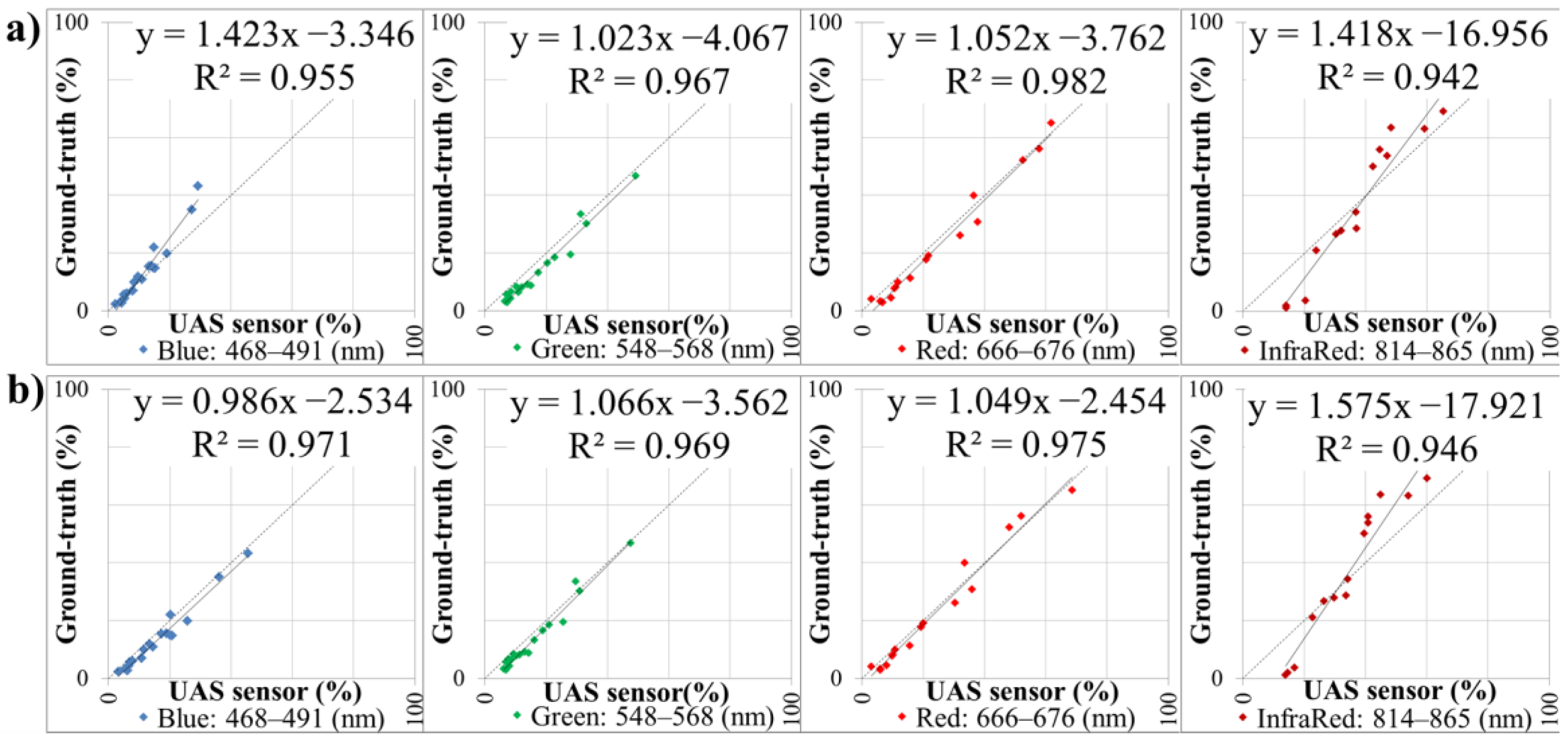
4.1. Fitting between Ground-Truth and Drone Data
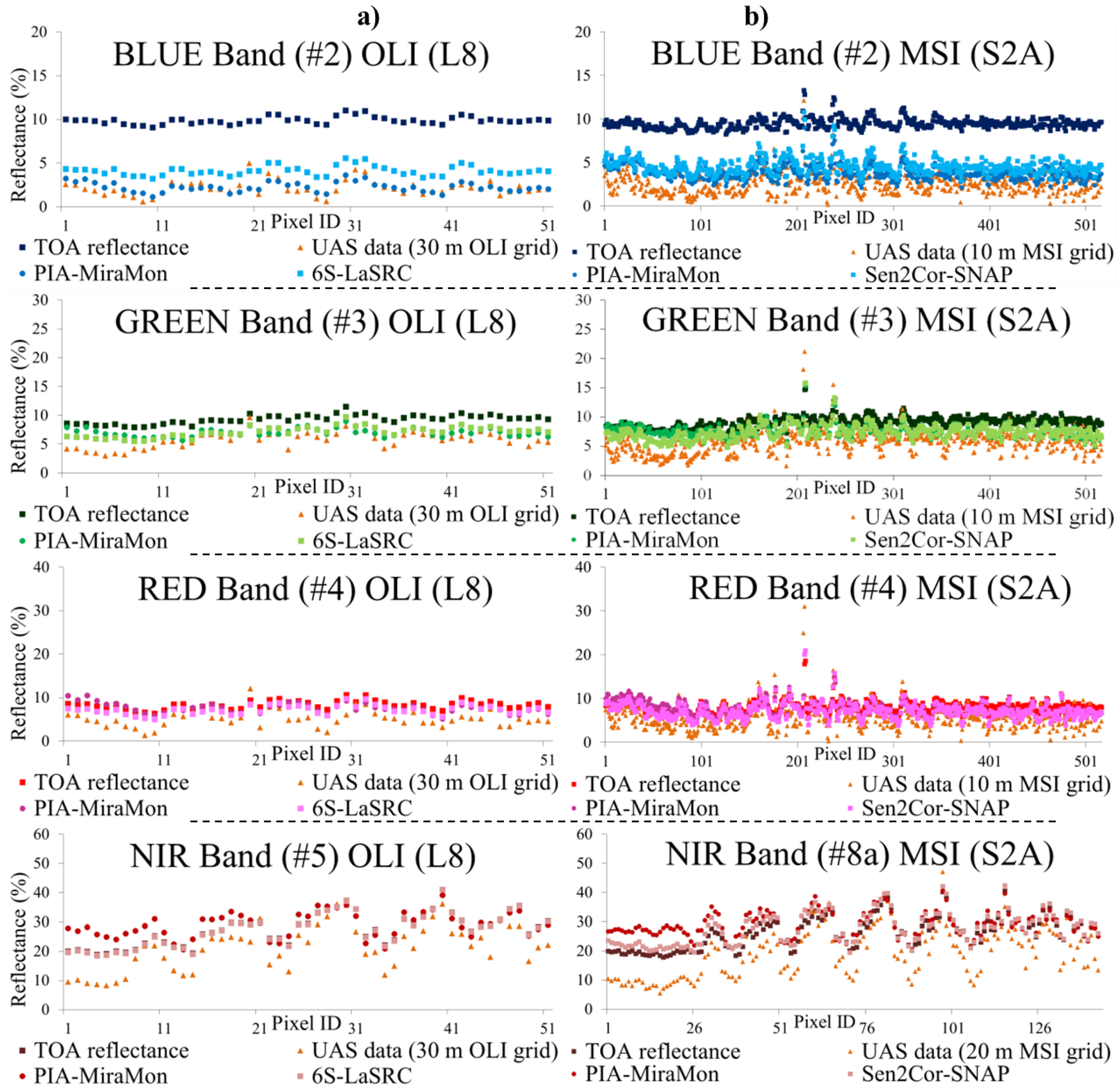
4.2. Fitting between the Drone Data and the Satellite Data
4.3. Fitting of the UAS-Based Satellite Radiometric Corrections with the Test Areas
4.4. Fitting between the Radiometric Correction of Almost Simultaneously Acquired L8 and S2 Data
5. Discussion
6. Conclusions
Author Contributions
Funding
Acknowledgments
Conflicts of Interest
References
- United Nations (UN). Transforming Our World: The 2030 Agenda for Sustainable Development. 21 October 2015. Available online: http://www.refworld.org/docid/57b6e3e44.html (accessed on 7 August 2018).
- Emery, W.J.; Camps, A. Introduction to Satellite Remote Sensing, 1st ed.; Emery, W., Camps, A., Eds.; Elsevier: Amsterdam, The Netherlands, 2017; p. 860. [Google Scholar]
- Diaz-Delgado, R.; Lucas, R.; Hurford, C. (Eds.) The Roles of Remote Sensing in Nature Conservation: A Practical Guide and Case Studies, 1st ed.; Springer: Cham, Switzerland, 2017; p. 318. [Google Scholar]
- Group on Earth Observation (GEO). Earth Observations in support of the 2030 Agenda for Sustainable development. Japan Aerospace Exploration Agency (JAXA) and GEO (EO4SDG Initiative). 2017, p. 19. Available online: https://www.earthobservations.org/documents/publications/201703_geo_eo_for_2030_agenda.pdf (accessed on 7 August 2018).
- GEOSS. GEOSS Evolution. Available online: http://www.earthobservations.org/geoss.php (accessed on 7 August 2018).
- National Aeronautics and Space Administration (NASA). Landsat Data Continuity Mission (LDCM). Available online: https://www.nasa.gov/mission_pages/landsat/main/index.html (accessed on 7 August 2018).
- European Space Agency (ESAa). ESA Sentinel Online. Sentinel-2 Mission. Available online: http://www.esa.int/Our_Activities/Observing_the_Earth/Copernicus/Sentinel-2 (accessed on 7 August 2018).
- European Space Agency (ESAb). ESA Sentinel Online. Sentinel-2 Mission Objectives. Available online: https://sentinel.esa.int/web/sentinel/missions/sentinel-2/mission-objectives (accessed on 7 August 2018).
- Li, J.; Roy, D.P. A Global Analysis of Sentinel-2A, Sentinel-2B and Landsat-8 Data Revisit Intervals and Implications for Terrestrial Monitoring. Remote Sens. 2017, 9, 902. [Google Scholar] [CrossRef]
- Liou, K.N. An Introduction to Atmospheric Radiation, 2nd ed.; Liou, K.N., Ed.; Academic Press: San Diego, CA, USA, 2002; p. 583. [Google Scholar]
- Nicodemus, F.E.; Richmond, J.C.; Hsia, J.J. Geometrical Considerations and Nomenclature for Reflectance; National Bureau of Standards, US Department of Commerce: Washington, DC, USA, 1977. Available online: http://physics.nist.gov/Divisions/Div844/facilities/specphoto/pdf/geoConsid.pdf (accessed on 7 August 2018).
- Riano, D.; Chuvieco, E.; Salas, J.; Aguado, I. Assessment of different topographic corrections in Landsat-TM data for mapping vegetation types. IEEE Trans. Geosci. Remote Sens. 2003, 41, 1056–1061. [Google Scholar] [CrossRef]
- Vermote, E.F.; Tanre, D.; Deuzé, J.L.; Herman, M.; Morcrette, J.-J. Second Simulation of the Satellite Signal in the Solar Spectrum, 6S: An Overview. IEEE Trans. Geosci. Remote Sens. 1997, 35, 675–686. [Google Scholar] [CrossRef]
- Vermote, E.; Justice, C.; Claverie, M.; Franch, B. Preliminary analysis of the performance of the Landsat 8/OLI land surface reflectance product. Remote Sens. Environ. 2016, 185, 46–56. [Google Scholar] [CrossRef]
- Richter, R.; Schläpfer, D. Atmospheric/Topographic Correction for Satellite Imagery (ATCOR-2/3 User Guide, Version 9.0.2, March 2016). 2016. Available online: http://www.rese.ch/pdf/atcor3_manual.pdf (accessed on 7 August 2018).
- Richter, R.; Louis, J.; Müller-Wilm, U. [L2A-ATBD] Sentinel-2 Level-2A Products Algorithm Theoretical Basis Document. Version 2.0. 2012, pp. 1–72. Available online: https://earth.esa.int/c/document_library/get_file?folderId=349490&name=DLFE-4518.pdf (accessed on 7 August 2018).
- Mueller-Wilm, U. Sen2Cor Configuration and User Manual V2.4; European Space Agency, 2017; pp. 1–53. Available online: http://step.esa.int/thirdparties/sen2cor/2.4.0/Sen2Cor_240_Documenation_PDF/S2-PDGS-MPC-L2A-SUM-V2.4.0.pdf (accessed on 7 August 2018).
- Claverie, M.; Masek, J. Harmonized Landsat-8 Sentinel-2 (HLS) Product’s Guide. v.1.3; 2017. Available online: https://hls.gsfc.nasa.gov/documents/ (accessed on 7 August 2018). [CrossRef]
- Skakun, S.V.; Roger, J.-C.; Vermote, E.; Masek, J.; Justice, C. Automatic sub-pixel co-registration of Landsat-8 Operational Land Imager and Sentinel-2A Multi-Spectral Instrument images using phase correlation and machine learning based mapping. Int. J. Digit. Earth 2017, 10, 1253–1269. [Google Scholar] [CrossRef]
- Mandanici, E.; Bitelli, G. Preliminary Comparison of Sentinel-2 and Landsat 8 Imagery for a Combined Use. Remote Sens. 2016, 8, 1014. [Google Scholar] [CrossRef]
- CEOS-WGCV. CEOSS Cal/Val Portal. Available online: http://calvalportal.ceos.org/ (accessed on 7 August 2018).
- Doxani, G.; Vermote, E.; Roger, J.-C.; Gascon, F.; Adriaensen, S.; Frantz, D.; Hagolle, O.; Hollstein, A.; Kirches, G.; Li, F.; et al. Atmospheric Correction Inter-Comparison Exercise. Remote Sens. 2018, 10, 352. [Google Scholar] [CrossRef]
- Padró, J.C.; Pons, X.; Aragonés, D.; Díaz-Delgado, R.; García, D.; Bustamante, J.; Pesquer, L.; Domingo-Marimon, C.; González-Guerrero, O.; Cristóbal, J.; et al. Radiometric Correction of Simultaneously Acquired Landsat-7/Landsat-8 and Sentinel-2A Imagery Using Pseudoinvariant Areas (PIA): Contributing to the Landsat Time Series Legacy. Remote Sens. 2017, 9, 1319. [Google Scholar] [CrossRef]
- Pons, X.; Solé-Sugrañes, L. A simple radiometric correction model to improve automatic mapping of vegetation from multispectral satellite data. Remote Sens. Environ. 1994, 45, 317–332. [Google Scholar] [CrossRef]
- McCoy, R.M. Field Methods in Remote Sensing, 1st ed.; McCoy, R.M., Ed.; The Guilford Press: New York, NY, USA, 2005; p. 159. ISBN 1-59385-080-8. [Google Scholar]
- Milton, E.J.; Schaepmann, M.E.; Anderson, K.; Kneubühler, M.; Fox, N. Progress in field spectroscopy. Remote Sens. Environ. 2009, 113, S92–S109. [Google Scholar] [CrossRef]
- Smith, G.M.; Milton, E.J. The use of the empirical line method to calibrate remotely sensed data to reflectance. Int. J. Remote Sens. 1999, 20, 2653–2662. [Google Scholar] [CrossRef]
- Colwell, R.N.; Ulaby, F.T.; Simonett, D.S.; Estes, J.E.; Thorley, G.A. Manual of Remote Sensing, 2nd ed.; Colwell, R.N., Ed.; American Society of Photogrammetry: Falls Church, VA, USA, 1983; Volume 2, p. 2440. ISBN 093729442X. [Google Scholar]
- Sánchez Alberola, J.; Oliver, P.; Estornell, J.; Dopazo, C. Estimación de variables forestales de Pinus Sylvestris L. en el contexto de un inventario forestal aplicando tecnología LiDAR aeroportada [Estimation of forest variables of Pinus Sylvestris L. in the context of a forestry inventory applying airborne LiDAR technology]. GeoFocus 2018, 21, 79–99. [Google Scholar] [CrossRef]
- Aasen, H.; Honkavaara, E.; Lucieer, A.; Zarco-Tejada, P.J. Quantitative Remote Sensing at Ultra-High Resolution with UAV Spectroscopy: A Review of Sensor Technology, Measurement Procedures, and Data Correction Workflows. Remote Sens. 2018, 10, 1091. [Google Scholar] [CrossRef]
- OPTIMISE. Innovative Optical Tools for Proximal Sensing of Ecophysiological Processes (ESSEM COST Action ES1309). Available online: https://optimise.dcs.aber.ac.uk/ (accessed on 7 August 2018).
- Mac Arthur, A.; Robinson, I. A critique of field spectroscopy and the challenges and opportunities it presents for remote sensing for agriculture, ecosystems, and hydrology. In Proceedings of the SPIE Remote Sensing for Agriculture, Ecosystems, and Hydrology, Toulouse, France, 14 October 2015. [Google Scholar]
- Iqbal, F.; Lucieer, A.; Barry, K. Simplified radiometric calibration for UAS-mounted multispectral sensor. European J. Rem. Sens. 2018, 51, 301–313. [Google Scholar] [CrossRef]
- Honkavaara, E.; Kaivosoja, J.; Mäkynen, J.; Pellikka, I.; Pesonen, L.; Saari, H.; Salo, H.; Hakala, T.; Marklelin, L.; Rosnell, T. Hyperspectral Reflectance Signatures and Point Clouds for Precision Agriculture by Light Weight UAV Imaging System. In Proceedings of the XII ISPRS Annals of Photogrammetry, Remote Sensing and Spatial Information Sciences, Melbourne, VIC, Australia, 25 August–1 September 2012; Volume I-7, pp. 353–358. [Google Scholar] [CrossRef]
- Matese, A.; Toscano, P.; Di Gennaro, S.F.; Genesio, L.; Vaccari, F.P.; Primicerio, J.; Belli, C.; Zaldei, A.; Bianconi, R.; Gioli, B. Intercomparison of UAV, Aircraft and Satellite Remote Sensing Platforms for Precision Viticulture. Remote Sens. 2015, 7, 2971–2990. [Google Scholar] [CrossRef] [Green Version]
- Adão, T.; Hruška, J.; Pádua, L.; Bessa, J.; Peres, E.; Morais, R.; Sousa, J.J. Hyperspectral Imaging: A Review on UAV-Based Sensors, Data Processing and Applications for Agriculture and Forestry. Remote Sens. 2017, 9, 1110. [Google Scholar] [CrossRef]
- Manfreda, S.; McCabe, M.; Miller, P.; Lucas, R.; Pajuelo Madrigal, V.; Mallinis, G.; Ben-Dor, E.; Helman, D.; Estes, L.; Ciraolo, G.; et al. On the Use of Unmanned Aerial Systems for Environmental Monitoring. Remote Sens. 2018, 10, 641. [Google Scholar] [CrossRef]
- Zabala, S. Comparison of Multi-Temporal and Multispectral Sentinel-2 and Unmanned Aerial Vehicle Imagery for Crop Type Mapping. Master of Science (MSc) Thesis, Lund University, Lund, Sweden, June 2017. [Google Scholar]
- MicaSense. MicaSense RedEdge™ 3 Multispectral Camera User Manual; MicaSense, Inc.: Seattle, WA, USA, 2015; p. 33. Available online: https://support.micasense.com/hc/en-us/article_attachments/204648307/RedEdge_User_Manual_06.pdf (accessed on 1 July 2018).
- Jhan, J.P.; Rau, J.Y.; Haala, N.; Cramer, M. Investigation of Parallax Issues for Multi-Lens Multispectral Camera Band Co-Registration. Int. Arch. Photogramm. Remote Sens. Spatial Inf. Sci. 2017, XLII-2/W6, 157–163. [Google Scholar] [CrossRef]
- Parrot Drones. Parrot Sequoia Technical Specifications. 2018. Available online: https://www.parrot.com/global/parrot-professional/parrot-sequoia#technicals (accessed on 7 August 2018).
- Fernández-Guisuraga, J.M.; Sanz-Ablanedo, E.; Suárez-Seoane, S.; Calvo, L. Using Unmanned Aerial Vehicles in Postfire Vegetation Survey Campaigns through Large and Heterogeneous Areas: Opportunities and Challenges. Sensors 2018, 18, 586. [Google Scholar] [CrossRef] [PubMed]
- Rumpler, M.; Daftry, S.; Tscharf, A.; Prettenthaler, R.; Hoppe, C.; Mayer, G.; Bischof, H. Automated End-to-End Workflow for Precise and Geo-accurate Reconstructions using Fiducial Markers. In Proceedings of the ISPRS Technical Commission III Symposium, Zurich, Switzerland, 5–7 September 2014; pp. 135–142. [Google Scholar] [CrossRef]
- Martínez-Carricondo, P.; Agüera-Vega, F.; Carvajal-Ramírez, F.; Mesas-Carrascosa, F.J.; García-Ferrer, A.; Pérez-Porras, F.J. Assessment of UAV-photogrammetric mapping accuracy based on variation of ground control points. Int J Appl Earth Obs. 2018, 72, 1–10. [Google Scholar] [CrossRef]
- Wang, C.; Myint, S.W. A Simplified Empirical Line Method of Radiometric Calibration for Small Unmanned Aircraft Systems-Based Remote Sensing. IEEE J. Sel. Top. Appl. Earth Obs. Remote Sens. 2015, 8, 1876–1885. [Google Scholar] [CrossRef]
- Pons, X.; Pesquer, L.; Cristóbal, J.; González-Guerrero, O. Automatic and improved radiometric correction of Landsat imagery using reference values from MODIS surface reflectance images. Int. J. Appl. Earth Obs. Geoinf. 2014, 33, 243–254. [Google Scholar] [CrossRef]
- OceanOptics. USB2000+ Fiber Optic Spectrometer Installation and Operation Manual; Ocean Optics, Inc.: Dunedin, FL, USA, 2010. [Google Scholar]
- OceanOptics. USB200+ Data Sheet; Ocean Optics, Inc.: Dunedin, FL, USA, 2006; Available online: https://oceanoptics.com/wp-content/uploads/OEM-Data-Sheet-USB2000-.pdf (accessed on 7 August 2018).
- Rees, W.G. Physical Principles of Remote Sensing, 3rd ed.; Rees, W.G., Ed.; Cambridge University Press: New York, NY, USA, 2013; p. 441. ISBN 978-1-107-00473-3. [Google Scholar]
- National Aeronautics and Space Administration (NASA). Landsat Science: A Lambertian Reflector. 2018. Available online: https://landsat.gsfc.nasa.gov/a-lambertian-reflector/ (accessed on 29 September 2018).
- Ponce-Alcántara, S.; Arangú, A.V.; Plaza, G.S. The Importance of Optical Characterization of PV Backsheets in Improving Solar Module Power. Available online: https://www.ntc.upv.es/documentos/photovoltaics/PVI26_Paper_03_NTC-UPV-7.pdf (accessed on 29 September 2018).
- Ciesielski, E.; MicaSense, Seattle, WA, USA. Personal communication, 2016.
- Agisoft LLC. PhotoScan User Manual, Professional Edition, Version 1.4.1. 2018. Available online: http://www.agisoft.com/pdf/photoscan-pro_1_4_en.pdf (accessed on 1 July 2018).
- Pons, X.; MiraMon. Sistema d’Informació Geogràfica i software de Teledetecció. Versió 8.1f [MiraMon. Geographical Information System and Remote Sensing Software. Version 8.1f]. Centre de Recerca Ecològica i Aplicacions Forestals, CREAF. Bellaterra. 2018. Available online: http://www.creaf.uab.cat/miramon/Index_usa.htm (accessed on 1 July 2018).
- Leica Geosystems. Leica Viva GS14 Technical Specifications. 2017. Available online: http://www.leica-geosystems.es/downloads123/zz/gpsgis/VivaGS14/brochures-datasheet/Leica_Viva_GS14_DS_es.pdf (accessed on 1 July 2018).
- ASPRS (American Society for Photogrammetry and Remote Sensing). ASPRS Positional Accuracy Standards for Digital Geospatial Data. Edition 1, Version 1.0.0. 2014. Available online: http://www.asprs.org/a/society/divisions/pad/Accuracy/ASPRS_Positional_Accuracy_Standards_for_Digital_Geospatial_Data_Edition1_V1_FinalDraftForPublication.docx (accessed on 1 July 2018).
- MicaSense. RedEdge Camera Radiometric Calibration Model. 2018. Available online: https://support.micasense.com/hc/en-us/articles/115000351194-RedEdge-Camera-Radiometric-Calibration-Model (accessed on 7 August 2018).
- National Aeronautics and Space Administration (NASA). Landsat Science, Spectral Response of the Operational Land Imager in-Band. 2018. Available online: http://landsat.gsfc.nasa.gov/preliminary-spectral-response-of-the-operational-land-imager-in-band-band-average-relative-spectral-response/ (accessed on 7 August 2018).
- United States Geological Survey (USGS). EarthExplorer Download Tool. 2018. Available online: https://earthexplorer.usgs.gov/ (accessed on 7 August 2018).
- United States Geological Survey (USGS). Landsat 8 Data Users Handbook–Section 5: Conversion of DNs to Physical Units. 2018. Available online: https://landsat.usgs.gov/landsat-8-l8-data-users-handbook-section-5 (accessed on 7 August 2018).
- European Space Agency (ESA). Copernicus Open Access Hub. Available online: https://scihub.copernicus.eu/dhus/#/home (accessed on 28 October 2017).
- European Space Agency (ESA) Sentinel Online, Sentinel-2A Document Library, Sentinel-2AA (S2A-SRF). 2017. Available online: https://earth.esa.int/web/sentinel/user-guides/sentinel-2-msi/document-library/-/asset_publisher/Wk0TKajiISaR/content/sentinel-2a-spectral-responses (accessed on 7 August 2018).
- United States Geological Survey (USGS). Landsat-8 Data User Handbook. Version 2.0; 2016. Available online: https://landsat.usgs.gov/landsat-8-l8-data-users-handbook (accessed on 21 September 2018).
- European Space Agency (ESA). Sentinel-2 Radiometric Performance. 2018. Available online: https://earth.esa.int/web/sentinel/technical-guides/sentinel-2-msi/performance (accessed on 21 September 2018).
- Gascon, F.; Bouzinac, C.; Thépaut, O.; Jung, M.; Francesconi, B.; Louis, J.; Lonjou, V.; Lafrance, B.; Massera, S.; Gaudel-Vacaresse, A.; et al. Copernicus Sentinel-2A Calibration and Products Validation Status. Remote Sens. 2017, 9, 584. [Google Scholar] [CrossRef]
- Chavez, P.S., Jr. An improved dark-object subtraction technique for atmospheric scattering correction of multispectral data. Remote Sens. Environ. 1988, 24, 459–479. [Google Scholar] [CrossRef]
- Schowengerdt, R.A. Remote Sensing, Models and Methods for Image Processing, 3rd Ed.; Schowengerdt, R.A., Ed.; Elsevier: San Diego, CA, USA, 2007; p. 560. ISBN 978-0-12-369407-2. [Google Scholar]
- Anniballe, R.; Bonafoni, S. A Stable Gaussian Fitting Procedure for the Parameterization of Remote Sensed Thermal Images. Algorithms 2015, 8, 82–91. [Google Scholar] [CrossRef] [Green Version]


| Manufacturer-Model | Size (mm) | Weight (g) | Design | Fiber Optic FOV (°) |
| OceanOptics USB2000+ | 89.1 × 63.3 × 34.4 | 190 | Czerny-Turner | 25 |
| Sensor manufacturer and type | Sensor CCD samples | Sampling interval (nm) | Input Focal Length (mm) | Fiber optic diameter (µm) |
| CCD Sony ILX511B | 2048 | 0.3 | 42 | 50 |
| Raw radiometric resolution (bits) and expanded dynamic range (DN) | Grating #2 Spectral range (nm) | FWHM (nm) | Signal to Noise Ratio @ 50 ms | Minimum Integration time (ms) |
| 8 (0–65,535) | 340–1030 | 1.26 | 250:1 | 1 |
| Manufacturer-MODEL | Size (mm) | Weight (g) | Raw Radiometric Resolution (Bits) and Expanded Dynamic Range (DN) | |
| MicaSense RedEdge | 121 × 66 × 46 | 150 | 12 (0–65,535) | |
| Sensor type | Sensor size (pixels) | Pixel size (µm) | Focal Length (mm) | Field of View (°) |
| CMOS | 1280 × 960 | 3.75 × 3.75 | 5.5 | 47.2 |
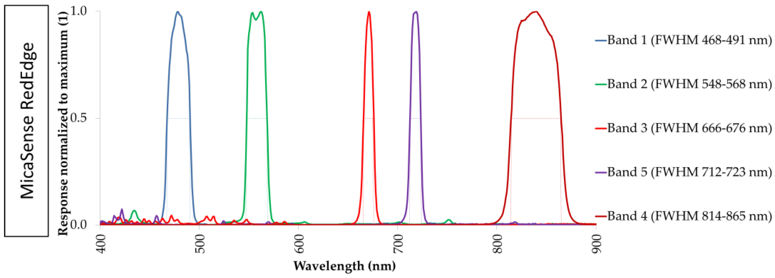
| #1 Blue FWHM (nm) | #2 Green FWHM (nm) | #3 Red FWHM (nm) | #4 Red-edge FWHM (nm) | #5 NIR FWHM (nm) |
| 468–491 | 548–568 | 666–676 | 712–723 | 814–865 |
| Acquisition Date | 21 April 2018 | |
|---|---|---|
| Study Area | 1°32′1.4″E, 41°56′59.3″N | |
| Platform | Landsat-8 | Sentinel-2A |
| Sensor | Operational Land Imager (OLI) | Multi Spectral Imager (MSI) |
| Bands | 10 | 13 |
| Aerosols | B1: 435.0 nm–451.0 nm (30 m) | B1: 432.7 nm–452.4 nm (60 m) |
| Blue | B2: 452.0 nm–512.1 nm (30 m) | B2: 459.8 nm–524.0 nm (10 m) |
| Green | B3: 532.7 nm–590.1 nm (30 m) | B3: 542.8 nm–577.6 nm (10 m) |
| Red | B4: 653.9 nm–673.3 nm (30) | B4: 649.3 nm–679.9 nm (10 m) |
| NIR(RedEdge) | B5: 697.3 nm–711.3 nm (20 m) | |
| NIR(RedEdge) | B6: 733.6 nm–747.3 nm (20 m) | |
| NIR(RedEdge) | B7: 773.5 nm–792.5 nm (20 m) | |
| NIR (wide) | B8: 782.5 nm–887.3 nm (10 m) | |
| NIR | B5: 850.5 nm–878.8 nm (30 m) | B8A: 854.5 nm–875.0 nm (20 m) |
| Water Vapor | B9: 935.4 nm–954.9 nm (60 m) | |
| Cirrus | B9: 1363.0 nm–1384.0 nm (30 m) | B10: 1359.0 nm–1388.1 nm (60 m) |
| SWIR1 | B6: 1566.5 nm–1651.2 nm (30 m) | B11: 1568.7 nm–1658.3 nm (20 m) |
| SWIR2 | B7: 2107.4 nm–2294.1 nm (30 m) | B12: 2112.9 nm–2286.5 nm (20 m) |
| Panchromatic | B8: 503.0 nm–676.0 nm (15 m) | |
| Thermal1 | B10: 10.60 µm–11.19 µm (100 m) | |
| Thermal2 | B11: 11.50 µm–12.51 µm (100 m) | |
| Acquisition time | 10:35:49 (UTC) | 10:56:29 (UTC) |
| Orbit-Scene | 198-031 | R051-TCG |
| Scene center | 41°45′19.2″, 1°16′28.2″ | 41°56′41.6″, 1°14′58. 2″ |
| Solar elevation | 55.67° (Scene center) 56.14° (Study area) | 57.73° (Scene center) 57.57° (Study area) |
| Solar Azimuth | 144.75° (Scene center) 147.32° (Study area) | 154.56° (Scene center) 153.80° (Study area) |
| View Zenith Angle | 7.26° (Study area) | 1.23° (Study area) |
| BLUE | GREEN | RED | NIR | |||||
|---|---|---|---|---|---|---|---|---|
| RMSE UAS Data vs. Data Source | OLI #2 (n = 51) | MSI #2 (n = 517) | OLI #3 (n = 51) | MSI #3 (n = 517) | OLI #4 (n = 51) | MSI #4 (n = 517) | OLI #5 (n = 51) | MSI #8a (n = 143) |
| TOA reflectance | 7.743 | 6.981 | 3.684 | 3.674 | 3.533 | 3.101 | 6.847 | 8.050 |
| PIA-MiraMon | 0.703 | 1.549 | 1.745 | 2.477 | 3.017 | 2.802 | 9.177 | 11.349 |
| Official products | 2.054 | 2.192 | 1.623 | 2.058 | 2.484 | 2.361 | 6.688 | 8.783 |
| RMSE PIA-MiraMon vs. Official products | 1.882 | 0.818 | 0.746 | 0.715 | 1.061 | 0.780 | 3.693 | 2.757 |
| BLUE | GREEN | RED | NIR | |||||
|---|---|---|---|---|---|---|---|---|
| RMSE Test Areas vs. Data Source | OLI #2 (n = 20) | MSI #2 (n = 207) | OLI #3 (n = 20) | MSI #3 (n = 207) | OLI #4 (n = 20) | MSI #4 (n = 207) | OLI #5 (n = 20) | MSI #8a (n = 57) |
| UAS-MiraMon | 0.712 | 0.745 | 1.000 | 1.230 | 1.871 | 2.018 | 7.530 | 6.760 |
| PIA-MiraMon | 0.585 | 1.366 | 1.746 | 1.867 | 3.130 | 2.373 | 8.528 | 7.281 |
| Official Products | 2.197 | 2.149 | 1.653 | 1.806 | 2.680 | 2.192 | 5.841 | 7.690 |
| RMSE (%) between Near Coincident L8 and S2 Images Corrected with the UAS-MiraMon Method | ||||
|---|---|---|---|---|
| Distance to UAS Central Scene (Number of Inter-Compared Pixels) | BLUE | GREEN | RED | NIR |
| 0–15 km (n = 681,950) | 0.621 | 0.741 | 0.919 | 1.664 |
| 15–30 km (n = 2,203,730) | 0.739 | 0.815 | 0.984 | 1.666 |
| TCG scene (n = 12,148,700) | 0.852 | 0.940 | 1.147 | 1.707 |
© 2018 by the authors. Licensee MDPI, Basel, Switzerland. This article is an open access article distributed under the terms and conditions of the Creative Commons Attribution (CC BY) license (http://creativecommons.org/licenses/by/4.0/).
Share and Cite
Padró, J.-C.; Muñoz, F.-J.; Ávila, L.Á.; Pesquer, L.; Pons, X. Radiometric Correction of Landsat-8 and Sentinel-2A Scenes Using Drone Imagery in Synergy with Field Spectroradiometry. Remote Sens. 2018, 10, 1687. https://0-doi-org.brum.beds.ac.uk/10.3390/rs10111687
Padró J-C, Muñoz F-J, Ávila LÁ, Pesquer L, Pons X. Radiometric Correction of Landsat-8 and Sentinel-2A Scenes Using Drone Imagery in Synergy with Field Spectroradiometry. Remote Sensing. 2018; 10(11):1687. https://0-doi-org.brum.beds.ac.uk/10.3390/rs10111687
Chicago/Turabian StylePadró, Joan-Cristian, Francisco-Javier Muñoz, Luis Ángel Ávila, Lluís Pesquer, and Xavier Pons. 2018. "Radiometric Correction of Landsat-8 and Sentinel-2A Scenes Using Drone Imagery in Synergy with Field Spectroradiometry" Remote Sensing 10, no. 11: 1687. https://0-doi-org.brum.beds.ac.uk/10.3390/rs10111687