On the Use of Dual-Doppler Radar Measurements for Very Short-Term Wind Power Forecasts

Abstract

Very short-term forecasts of wind power provide electricity market participants with extremely valuable information, especially in power systems with high penetration of wind energy. In very short-term horizons, statistical methods based on historical data are frequently used. This paper explores the use of dual-Doppler radar observations of wind speed and direction to derive five-minute ahead deterministic and probabilistic forecasts of wind power. An advection-based technique is introduced, which estimates the predictive densities of wind speed at the target wind turbine. In a case study, the proposed methodology is used to forecast the power generated by seven turbines in the North Sea with a temporal resolution of one minute. The radar-based forecast outperforms the persistence and climatology benchmarks in terms of overall forecasting skill. Results indicate that when a large spatial coverage of the inflow of the wind turbine is available, the proposed methodology is also able to generate reliable density forecasts. Future perspectives on the application of Doppler radar observations for very short-term wind power forecasting are discussed in this paper.

1. Introduction

The increasing participation of offshore wind power in electricity markets continuously poses challenges for ensuring grid stability and power quality, especially due to the enhanced variability of offshore wind power in short scales [1]. A recent project in Germany allows wind farms to downregulate their power to participate in the reserve market, where reserves are calculated in one-minute intervals [2]. During the pilot phase of the project, the standard deviation of the prediction error of the possible power is required to be less than ± 5%. These changes in grid regulations, driven by faster temporal responses of the grid, show the importance of improving wind power forecasts with shorter horizons and higher temporal resolutions in order to reduce the costs associated with operating the grid and minimize balancing reserves.

Reliable very short-term forecasts of wind power also benefit electricity market participants since they allow them to be more competitive in intraday markets [3]. As electricity markets are becoming more flexible with the use of intraday gate closure times as short as five minutes [4], the technical challenge arises on how to generate accurate very short-term wind power forecasts.

Very short-term or minute-scale forecasts of wind power (<60 min) are usually based on statistical time-series models. For larger horizons, numerical weather prediction (NWP) models are more accurate [5]. Examples of very short-term forecasts of wind speed and power using time series methods can be found in [6,7,8]. Very short-term forecasts of wind speed and power are often based on machine learning methods such as artificial neural networks [9] or Markov chain models [10,11], which are trained with historical data. Alternatively, combinations of different models (known as hybrid models) have been proposed to overcome the deficiencies of single models [12]. Parallel to the development of single point or deterministic forecasting models, the use of probabilistic forecasts, which include information about the uncertainty associated with the predicted events, has increased. Examples of very short-term probabilistic forecasts of wind power using statistical methods can be found in [13,14]. These probabilistic forecasts are known as predictive densities or probability distributions and provide important information for making risk-based decisions [15].

Over the last two decades, the use of remote sensing measurements such as long-range lidars [16] has been extended in the wind industry. These systems are capable of measuring wind speed and direction (under certain assumptions) up to 30 km [17]. Unlike conventional wind measurements from met-mast or satellites, they present an adequate trade-off between temporal and spatial resolution for wind farm applications. However, the prediction horizon of a remote sensing-based forecasting model is limited by the maximum range of the remote sensing measurements and also influenced by meteorological conditions [18]. Indeed, publications on the use of long-range lidar measurements for wind energy applications have reported measurements with a maximum range of less than ten kilometers [19,20,21]. Despite those limitations, a recent contribution showed that a lidar-based forecasting technique can provide better results than conventional statistical benchmarks when forecasting near-coastal winds with lead times of five minutes [22].

Alternatively, the use of weather radars has also been investigated for short-term (minutes to few hours) forecasting of wind power, due to its appropriate spatial and temporal resolution. Trombe et al. [23] introduced the use of ground-based weather radars, which measure precipitation reflectivity, for predicting large power fluctuations in the offshore wind farm Horns Rev. As precipitation fields are highly correlated to strong wind speed fluctuations, weather radar systems show a high potential in anticipating strong power fluctuations at offshore sites [24].

The use of wind speed and direction observations from Doppler radars for wind energy applications has recently been explored. Wind farm operational data was coupled with wind fields derived from dual-Doppler (two synchronized Doppler radars) measurements to further investigate wind farm wake effects and evaluate wake modelling [25]. Dual-Doppler (DD) radar measurements of the wake behind an offshore wind farm were also reported in [26]. Power performance studies [27] and ramp events detection [28] were also documented using DD radar measurements.

In [29], the authors introduced a methodology that uses DD radar measurements as input for predicting the average aggregated power of seven offshore wind turbines in a probabilistic framework. This paper extends the methodology presented in [29] to predict the power generated by individual wind turbines and analyses the characteristics of DD radar measurements for very short-term forecasts of wind power. Thus, the main goals of this paper are (i) the description of a methodology that uses fully resolved DD radar measurements to create probabilistic forecasts of wind power, (ii) its evaluation on seven wind turbines in an offshore wind farm with a very short-term horizon of five minutes and (iii) the assessment of the measurement characteristics and quality aspects of DD radar observations for very short-term forecast of wind power.

Our paper is organised as follows: first, we introduce the DD radar system along with the measurement campaign in Section 2. The forecasting methodology is detailed in Section 3. We investigate the use of probabilistic and deterministic forecasts of power for individual wind turbines and a row of wind turbines in Section 4. A discussion on the use of DD radar observations for wind power forecasting is given in Section 5. Conclusions are drawn in Section 6.

2. Data Description

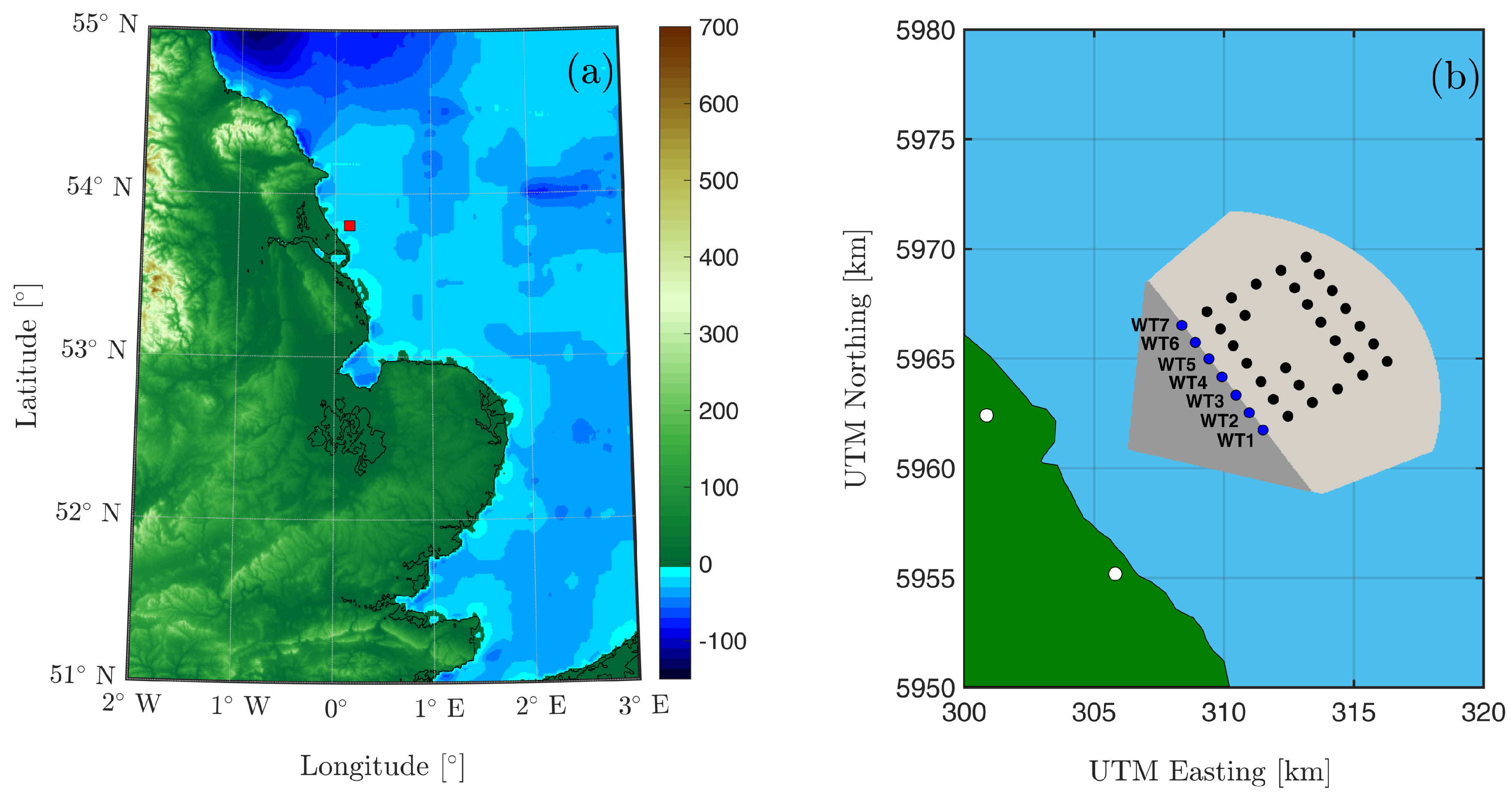
The data used in this analysis was collected during the BEACon research and development (R&D) project conducted by Ørsted [26]. The BEACon measurement campaign started in July 2016, lasting until the spring of 2018. Two Doppler radar units scanned the flow within and surrounding the Westermost Rough offshore wind farm in the North Sea (Figure 1a,b). 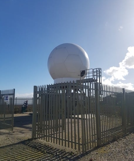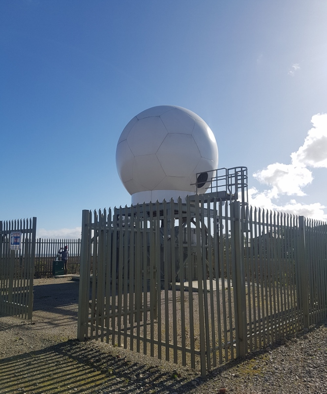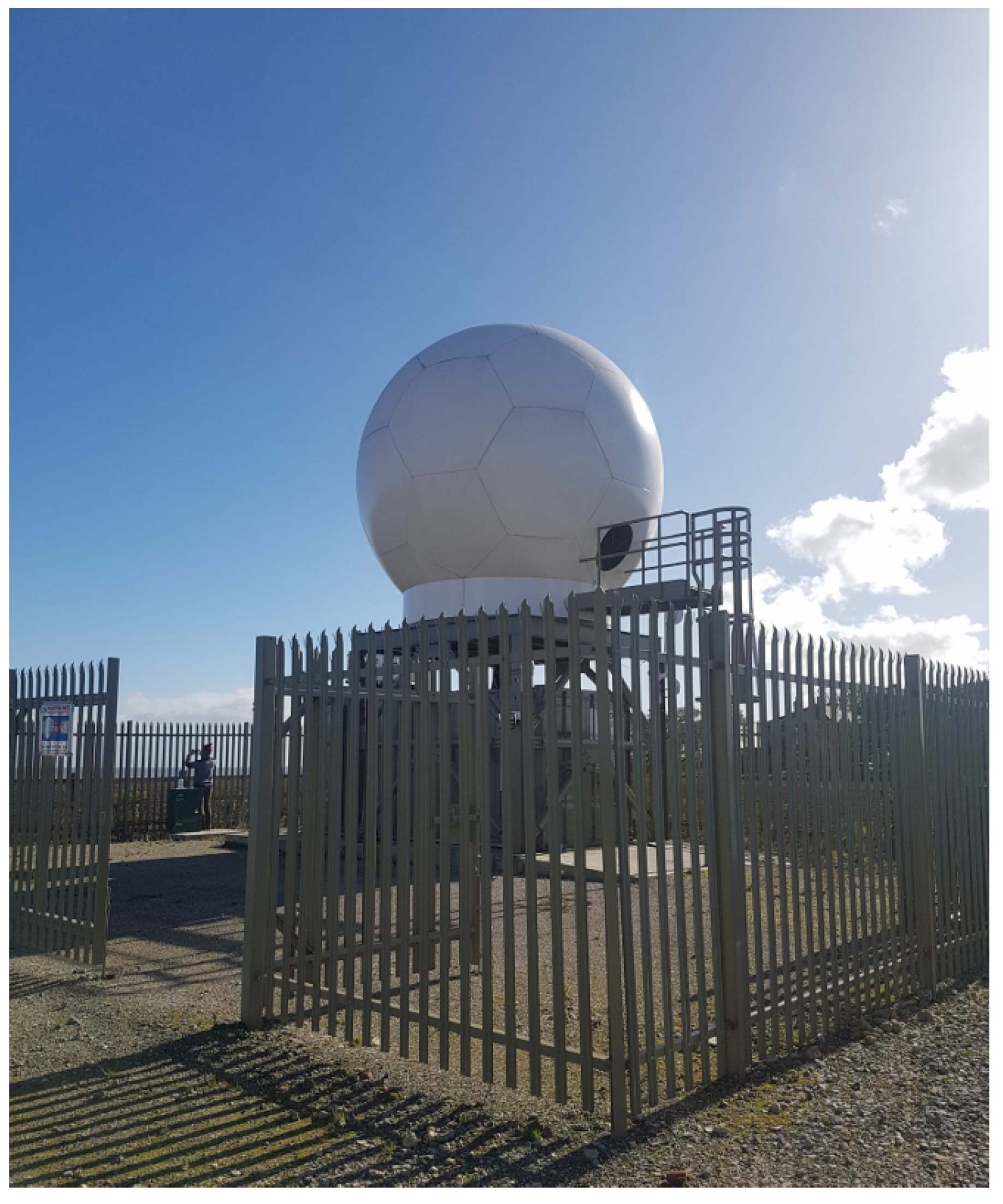Westermost Rough is composed of 35 turbines with a hub height of 106 m, a rotor diameter (D) of 154 m and a rated power of 6 MW. The two Doppler radars (Figure 2) are located at the shoreline 8 km from the closest wind turbines (Figure 1b). The last row of turbines is 14 km from the coast.

The DD radar system [26] was configured to obtain volumetric wind field measurements with a temporal resolution of roughly one minute. Each radar scanned a 60${}^{\circ }$ sector at 13 different elevation tilts, ranging from 0.2 to 1.4${}^{\circ }$. During the performance of a one-minute volumetric measurement cycle, flow homogeneity is assumed. The radars measured the flow with a spatial resolution of 0.5${}^{\circ }$ in the azimuthal direction, given by the beam width, and 15 m along the beam direction. To retrieve the two horizontal wind speed components, the line-of-sight (radial) velocity measurements from the two radars are interpolated into a three-dimensional Cartesian grid over the overlapping region measured by the radars (Figure 1b). It is assumed that no vertical flow component exists. The maximum range of the radar measurements is 32 km. After interpolation into the Cartesian grid, the final DD volumetric wind fields have a spatial horizontal resolution of 50 m and vertical resolution of 25 m. The accuracy of the radial velocity measurements of one of the Doppler radars has been validated in a measurement campaign using a scanning lidar, which had been previously calibrated with an anemometer. Results indicate a good correlation between the Doppler radar and the scanning lidar measurements [30]. The uncertainty in the dual-Doppler wind speed data is currently being quantified and will be reported elsewhere.

A sample of 2795 one-minute DD radar measurements during south-westerly winds was made available for this study. Those periods were continuously collected during several hours on 11 days between November 2016 and February 2017 and correspond to free-flow conditions (DD wind direction: 191.7–281.7${}^{\circ }$) for the first row of wind turbines (Figure 1b). We focus our analysis only on these wind turbines to avoid the additional complication of wake effects. The horizontal spacing of those wind turbines ranges from 5.92D to 6.43D. 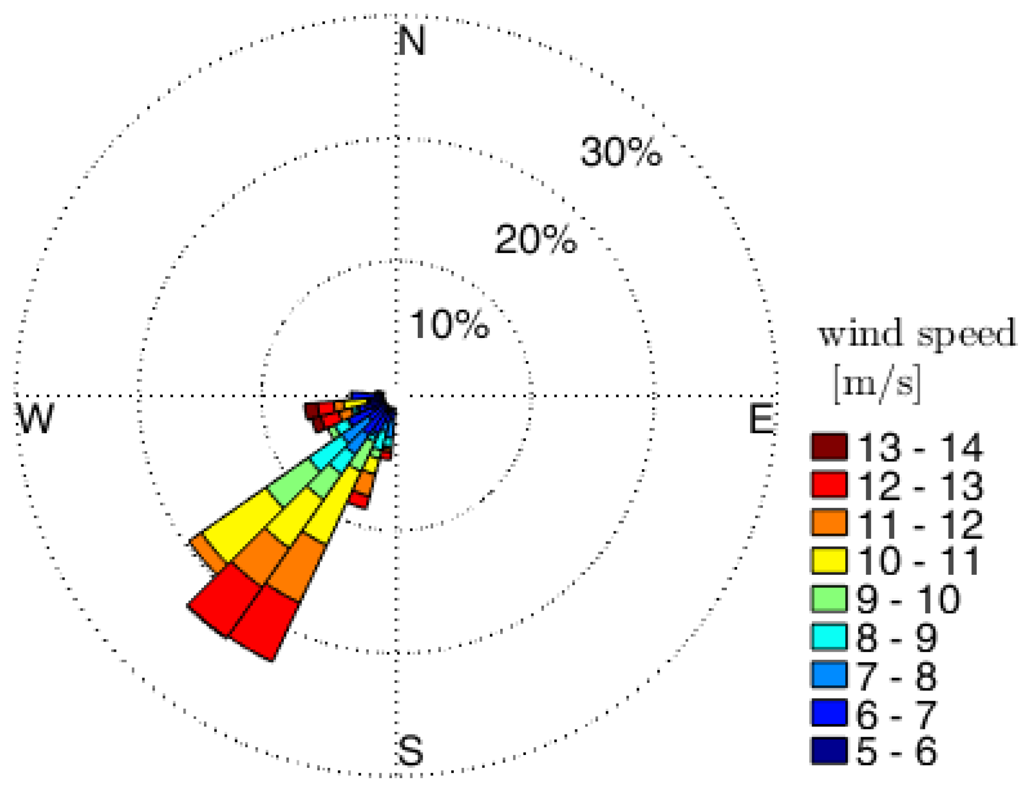The DD radar images were filtered for periods with spatial availability greater than 90% in the area corresponding to the inflow zone of the first row of wind turbines (dark gray shadowed area in Figure 1b). Only continuous periods of at least 20 min were considered. With these criterion applied, a total number of 1134 one-minute DD radar wind fields, with a mean spatial availability in the inflow area of 98.4%, were further investigated. During these periods, mean wind speeds at 100 m height (averaged over the radar domain) in the range of 5–14 m/s with a prevailing south-southwesterly direction were observed (Figure 3).

In addition to the DD wind field data, power data from the wind turbines’ supervisory control and data acquisition (SCADA) system is used to derive the wind turbine power curve and to validate the performance of the forecast. The power data with a frequency of 1 Hz is averaged every minute and temporally synchronized with the DD data. Periods with start-ups, shut-downs and abnormal performance such as power curtailment, power boosting and downtimes have been filtered.

3. Forecasting Methodology

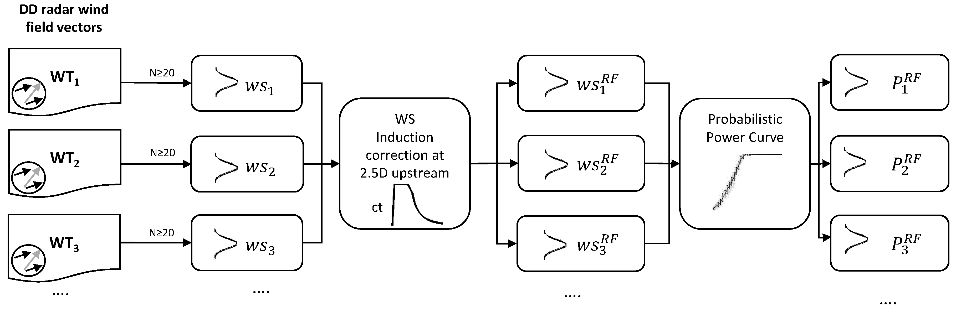
The forecasting methodology presented here uses fully-resolved DD wind field measurements as input to derive probabilistic forecasts of wind power. Figure 4 outlines the proposed methodology. To calculate a remote sensing-based forecast (RF) of power for the ith wind turbine $P_i^{RF}$ at a future time $t+k$, we need first to estimate the density forecast of the hub height wind speed $w{s}_i^{RF}$ at instant $t+k$. Then, the predictive density of wind speed at each rotor is transformed to power density by means of a probabilistic power curve. Due to the prevailing wind direction of the available data set and the particular measurement setup of the BEACon project focusing on wake effects, we forecast wind power output with a five-minute prediction horizon, i.e., five-steps ahead (k = 5). Here, we first introduce how the predictive densities of wind speed are estimated.

3.1. Predictive Wind Speed Densities

The probabilistic forecast of wind speed is based on a Lagrangian persistence technique widely applied in probabilistic forecasts of precipitation [31,32]. The principle underlying this method is the persistence of moving radar precipitation patterns. Our model uses wind speed information measured by the DD radar system at 100 m height to create the probabilistic forecast of wind speed. Thus, given a DD radar observed wind field at any given time t, the model propagates the horizontal wind field vectors with their respective trajectories defined by their local wind speed and direction for a duration k. The probabilistic wind speed advection forecast is constructed under the following premises: During the prediction horizon, (i) the observed DD radar wind field vectors maintain a constant horizontal trajectory (ii) mass conservation, vorticity and diffusion are neglected.

A simple approach to generate the predictive wind speed densities $w{s}_i$ at time $t+k$ at the target wind turbine is to search in the surroundings of the wind turbine for the velocity vectors advected during the forecast horizon. The ensemble of the magnitude of the advected velocity vectors comprises the distribution of wind speeds or predictive densities of wind speed.

The forecasting location or point of interest is defined as an area of influence $A_i$ encompassing the target wind turbine. We only consider the wind vectors from the DD scan at 100 m that will reach the area of influence within a time window of $\tau$ = 60 s centred around the forecast horizon. Thus, the basis of our probabilistic very short-term forecast of wind speed is the cloud of points or observations that fall inside the defined spatio-temporal window. For a forecasting horizon of five minutes, as it is the case here, we consider the wind field vectors found within the area of influence between 4.5 min and 5.5 min after the forecast is issued, under the Lagrangian persistence hypothesis.

To evaluate the predictive wind speed densities, we compare them with the DD wind speeds observed in front of the rotor (at 100 m height) of the considered wind turbines. Close to the rotor, a reduction of wind speed is experienced due to the extraction of axial momentum of the flow. The axial induction factor a expresses the velocity reduction at the rotor and can be defined in terms of the thrust coefficient $C_T$ by:

$$a=\frac{1}{2}\left(1-\sqrt[]{1-C_T}\right).$$

(1)

The International Electrotechnical Commission (IEC) standard for power curve measurements [33] recommends rotor wind speed observations to be measured 2.5D upstream of the rotor. At this distance, the flow is assumed to be “outside” the induction zone. The power curve used in this analysis and introduced in Section 3.2 is based on DD measurements at this distance, at the height of 100 m. Wind tunnel measurements have shown, however, that wind speed deficits due to the rotor blockage effect extend to 3D and beyond upstream of the wind turbine [34]. In considering the velocity reduction due to the induction zone in front of the rotor, we correct our wind speed distributions $w{s}_i$ using Equation (2), [34], at the distance of $x=-2.5D$ upstream of the wind turbine, where x is the spatial coordinate in the longitudinal flow direction. In our case, $U_{\infty }$ refers to the predicted DD wind speed $w{s}_i$ based on observations upstream (or in the undisturbed zone) and U (here $w{s}_i^{RF}$) denotes the wind speed at the distance of 2.5D upstream of the rotor. As mentioned before, $w{s}_i^{RF}$ will be transformed into power by using a power curve based on measurements at this distance. The induction factor is obtained from Equation (1), using the $C_T$ given by the manufacturer’s thrust curve at each wind speed level. For an induction factor a = $\frac{1}{3}$, the correction factor at $x=-2.5D$ equals 0.994, which is close to unity:

$$\frac{w{s}_i^{RF}}{w{s}_i}=\frac{U}{U_{\infty }}=1-a\left(1+\frac{2x}{D}{\left(1+{\left(\frac{2x}{D}\right)}^2\right)}^{-0.5}\right).$$

(2)

3.1.1. Optimization of the Wind Turbine Area of Influence

To optimize the probabilistic forecasting methodology, we conducted a sensitivity analysis on the area of influence encompassing the target wind turbine, as introduced in [29]. The area of influence $A_i$ is defined as a circle centred at the wind turbine (Figure 5c). The optimization criterion is the minimization of the average continuous ranked probability score (CRPS) of the wind speed predictions, after correcting for induction effects of the wind turbines in the first row. The continuos ranked probability score (crps) evaluates the spread of the predictive densities in regard to the observation [35] and is given by:

$$\mathrm{crps}\left(F,x_0\right)={\int }_{-\infty }^{\infty }{\left[F\left(x\right)-\theta (x-x_o)\right]}^{2}dx,$$

(3)

where F is the cumulative distribution function of the predictive density (in our case $w{s}_i^{RF}$), $x_0$ is the observation (here $w{s}_i^{2.5D}$) and $\theta$ is the Heaveside step function which takes the value 1 when $x\ge x_o$ and 0 otherwise. If the predictive density is reduced to a point forecast, then the crps can be understood as the absolute error. The lower the crps, the better the density forecast. For a skillful forecast, crps is close to zero, as F approximates the Heaviside step function of the observation. CRPS is given by:

$$\mathrm{CRPS}=\frac{1}{T}\sum _{j=1}^T\mathrm{crps}\left(F_j,x_{o,j}\right),$$

(4)

where T refers to the number of samples analysed. To optimize the area of influence, we use wind speed densities predicted one-minute ahead (k = 1), as we want to optimize the area of influence with predictions close to the real distribution of wind speeds in front of the rotor.

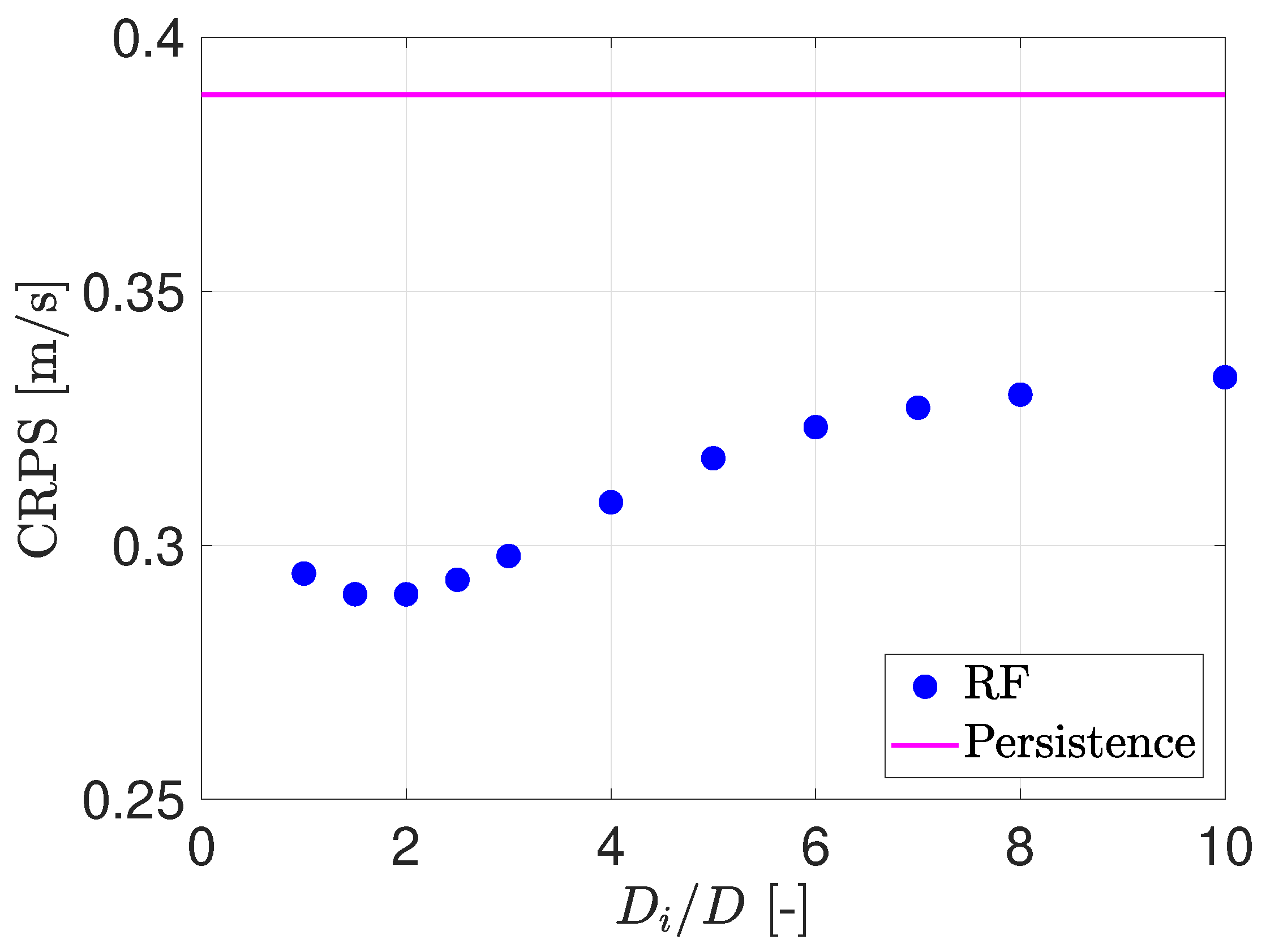
Figure 6 depicts the CRPS for different areas of influence, in terms of number of rotor diameters D. Here, we consider samples with a minimum number of wind field vectors $N_{\min }$ = 20 to estimate the predictive densities, following [29]. A total of T = 10,447 predictions are considered for the sensitivity analysis. The figure also depicts the CRPS for a wind speed distribution estimated with the probabilistic extension of the forecasting model persistence. Persistence is the most often employed forecasting benchmark, which uses the last available measurement at time t, as the prediction at time $t+k$, and is known for being difficult to outperform for short horizons [5]. As we want to compare our model to a probabilistic prediction, we consider a persistence distribution using the persistence point and the 19 previous forecasting errors, as defined in [36]. The CRPS for the predictions based on the DD observations is smaller than for persistence. A decrease in the CRPS value can be observed when increasing the diameter of the area of influence up to 2D. Further increase of the area of influence shows no improvement. An area of influence larger than the optimum appears to extend the temporal and spatial characteristics of the wind speed distribution, which seem to be no longer representative of the sampling effect of the rotor. At the same time, a smaller area of influence than the optimum is not able to capture the distribution of wind speeds characteristic of the rotor.

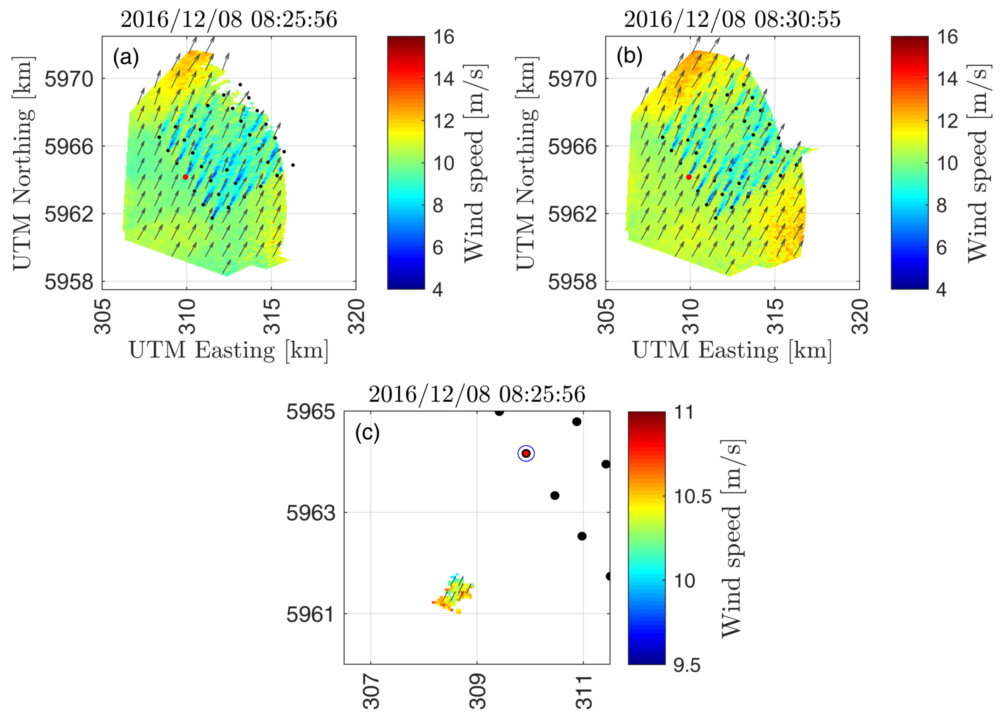
Based on the results of the sensitivity analysis of the area of influence, we use an area of influence with a diameter of 2D, for the results presented below. Figure 5c shows an example of the cloud of wind field vectors that will reach the area of influence of the wind turbine $WT4$ (in red) in 5 min ± 30 s. The wind fields at the time that the prediction is issued at and validated are illustrated in Figure 5a,b, respectively. The predicted wind speed distribution after implementing the correction due to the induction zone, along with its mean and the observed DD wind speed 2.5D upstream of the rotor at the validation time are depicted in Figure 7a.

3.1.2. Evaluation of Predicted Wind Speeds

Five-minute ahead single point predicted wind speeds $w{s}_i^{RF}$ are evaluated by comparison with the wind speeds observed 2.5D upstream of the turbine rotor $w{s}_i^{2.5D}$. Following the perspective of [36] and [13], the optimal single point predictor should be chosen from the predictive densities according to the target metric. Given that the focus of the paper is on evaluating the root-mean-square error (RMSE) of the predicted variables, the mean of the distribution is considered. 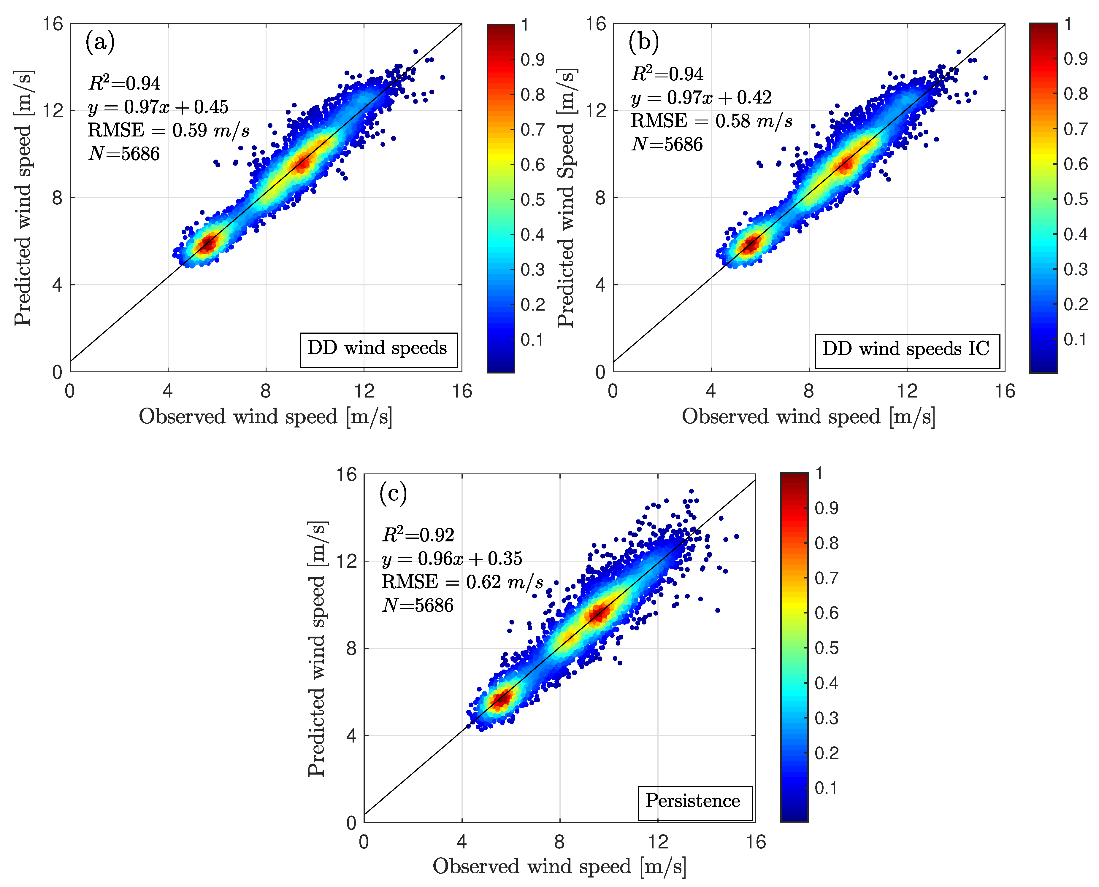Figure 8a–c compare the wind speeds observed 2.5D upstream of the turbine rotor with the mean of the predictive wind speed densities forecasted five minutes ahead, before and after applying the wind speed correction due to induction effects, and for the persistence method, respectively. The correction of wind speeds considering the induction effects improves the RMSE by 2%. Relative to persistence there is an improvement of 6%. In general, a high correlation is found between the predicted and the observed wind speeds. For wind speeds below 6 m/s, the DD predicted mean wind speeds (including the induction correction) overestimate the DD wind speeds 2.5D upstream by an average of 0.32 m/s. For wind speeds in the range 6–10 m/s, the predicted wind speeds exceed the DD wind speeds 2.5D upstream by an average of 0.15 m/s. Over 10 m/s, this difference is 0.12 m/s. Those differences are attributed, among others, to the assumption of the persistence of the wind field trajectories during the forecasting horizon and to the radar uncertainty.

Although this work focuses on predicting coastal winds, we are not considering the effects of the wind speed gradient present at the discontinuity between the land and the sea, which increases the uncertainty in the predictions. Studies on coastal gradients [37] have reported velocity reductions between 4% and 8% from 3 km to 1 km from the shore. Over 3 km from the coast, velocity gradients of 0.5%/km have been observed for different offshore sites [38]. Future work should include corrections for wind speeds due to coastal effects.

3.2. Predictive Wind Power Densities

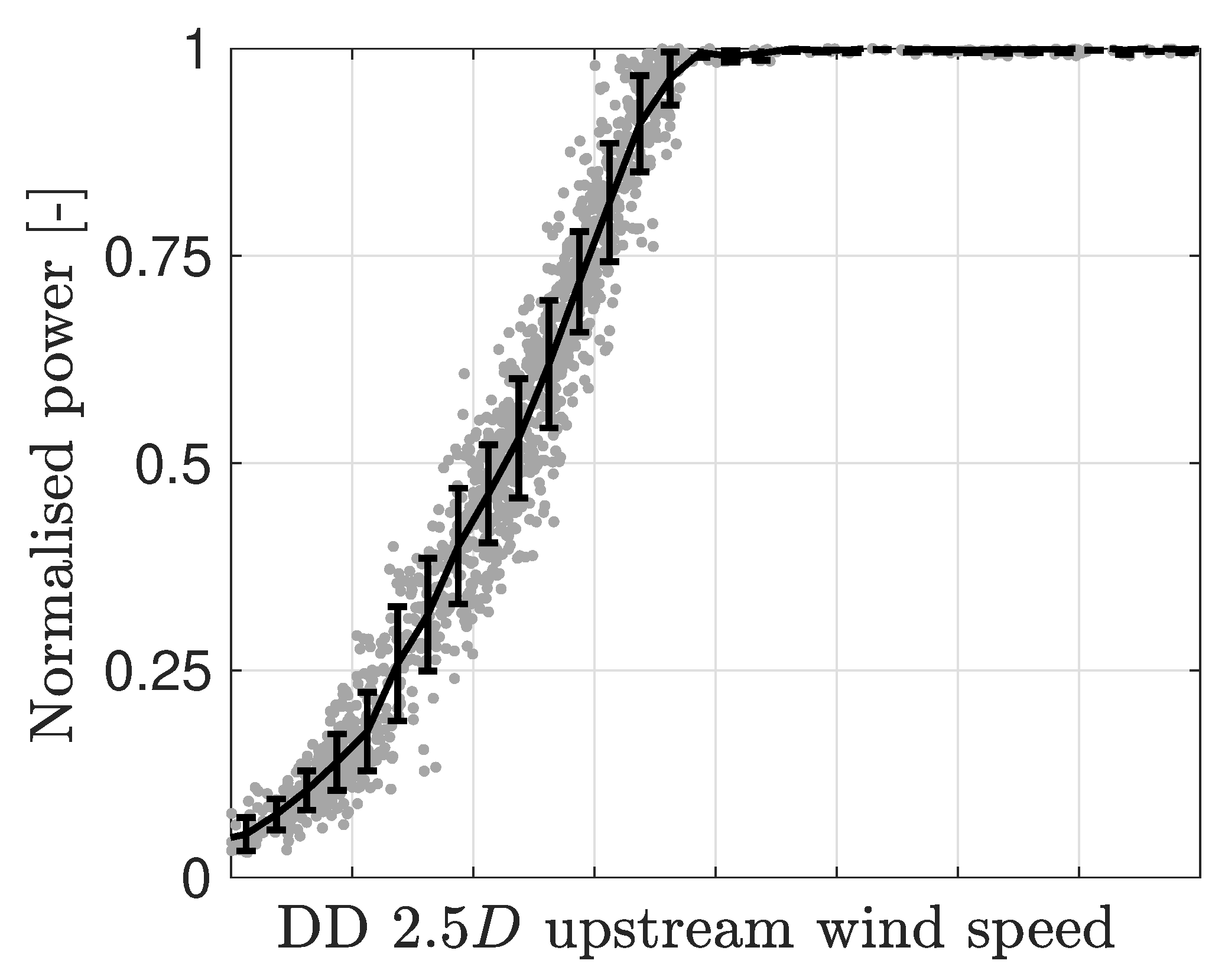
To estimate the predictive wind power densities $P_i^{RF}$, we transform the predictive wind speed densities $w{s}_i^{RF}$ into power densities using a probabilistic wind turbine power curve. Wind turbine power curves are normally built using ten-minute averages of wind speed and power, following an IEC standard [33]. Since our goal is to forecast wind power with a frequency of one minute, we derive the power curve from the one-minute DD wind speeds observed 2.5D upstream of the rotor of the considered wind turbines (Figure 9). This power curve is representative of an undisturbed inflow as only free-flow sectors are considered. The resulting power curve presents an irregular degree of variance for different wind speed levels, as shown in Figure 9. This is characteristic of a power curve constructed with high frequency data [39]. To include the uncertainty of the power curve in our forecasting model, a probabilistic power curve is built. First, we collect the power data into wind speed bins of 0.5 m/s width. Next, we estimate the empirical cumulative distribution function ($ecdf$) of the wind turbine power for each wind speed bin. We apply a resampling technique with replacement (bootstrap) [40] to derive the wind power predictive distributions, as wind speed predictive densities are based on an irregular number of wind field vectors. Thus, for each wind speed distribution, a total of 10,000 random values, out of the original $ecdf$ of the predicted wind speed distributions, are selected. With the resulting set of wind speed values, the predictive densities of power are derived by random selection from the power $ecdf$ associated to each wind speed bin. The estimated $ecdf$ of the predictive density of power for $WT4$, for the example introduced in Figure 5, is shown in Figure 7b.

4. Results

We assess the predictive performance of the RF model in terms of single point and probabilistic forecasts. Five-minute ahead predictions of power from the wind turbines of the first row and its aggregation are evaluated. The forecasting skill of the RF model is compared with the benchmarks persistence and climatology, which are described below. An analysis of the influence of the radar spatial availability on the performance of the RF model is also included.

4.1. Probabilistic Forecast Evaluation

To evaluate our probabilistic forecast, we follow Gneiting guidelines [35]. A probabilistic forecast aims at maximizing the sharpness of the predictive distributions under the constraint of calibration. Sharpness refers to the spread of the predictive distributions and is only a property of the forecasting variable. Calibration, however, is a joint property of the forecasts and observations and indicates the statistical consistency between the predictive distributions and the observed values. To evaluate the skill of the RF model we compare its sharpness and calibration with the probabilistic version of persistence and the climatology benchmarks. Climatology is the most common benchmark to assess climatological variables and can be understood as the average of the variable during a long period. Here, we define the climatology distribution as the probability distribution of all available SCADA power measurements. We derive the persistence distribution, defined in Section 3.1.1, using the persistence point forecast and the 19 most recent consecutive observed values of the persistence error, as described in [36].

4.1.1. Individual Wind Turbine Power

The overall performance of the predictive power densities of the seven wind turbines is assessed with the CRPS, previously defined in Section 3.1.1, but in this case using power. CRPS addresses both calibration and sharpness. Due to the reduced availability of time stamps with simultaneous measurements for the seven wind turbines, we first explore the results for all measurements available for each wind turbine. The respective results are given in % of nominal power $P_n$ (

Table 1. Average continous ranked probability score (CRPS), in % of the nominal capacity ($P_n$), of the five-minute ahead power forecasts for the seven wind turbines evaluated. Results are shown for the remote sensing-based forecast (RF), persistence and climatology benchmarks. Upper row presents the results for all available measurements (T) of each wind turbine. Lower row provides the results for all simultaneous available measurements. Minimum values are shown in bold.

		$\mathit{WT}\mathbf{1}$	$\mathit{WT}\mathbf{2}$	$\mathit{WT}\mathbf{3}$	$\mathit{WT}\mathbf{4}$	$\mathit{WT}\mathbf{5}$	$\mathit{WT}\mathbf{6}$	$\mathit{WT}\mathbf{7}$
	T	596	903	997	983	960	846	608
	RF	5.11	4.06	3.92	4.57	4.50	4.29	4.82
CRPS [%]	Persistence	5.37	4.98	5.04	5.07	4.96	4.88	4.85
	Climatology	17.93	17.45	17.32	17.15	17.07	16.96	16.79
	T	343	343	343	343	343	343	343
	RF	6.42	5.03	4.83	5.27	4.76	4.39	4.76
CRPS [%]	Persistence	6.12	5.79	5.63	5.76	5.76	5.85	5.91
	Climatology	16.78	16.31	15.58	15.37	15.32	15.03	14.94

, upper row). In general, the CRPS of the predictions with the RF model for individual wind turbines outperforms persistence and climatology. When evaluating the predictions made with the climatology and persistence models, a similar CRPS is found for each wind turbine, except for $WT1$ which shows a worse performance in general. We assume that these differences stem from the different operational behaviour of the wind turbines. In contrast to the benchmarks, the CRPS of the RF model shows higher variability among the wind turbines. Wind turbines $WT1$ and $WT7$ show higher CRPS values than the other wind turbines whilst $WT3$ performs best. 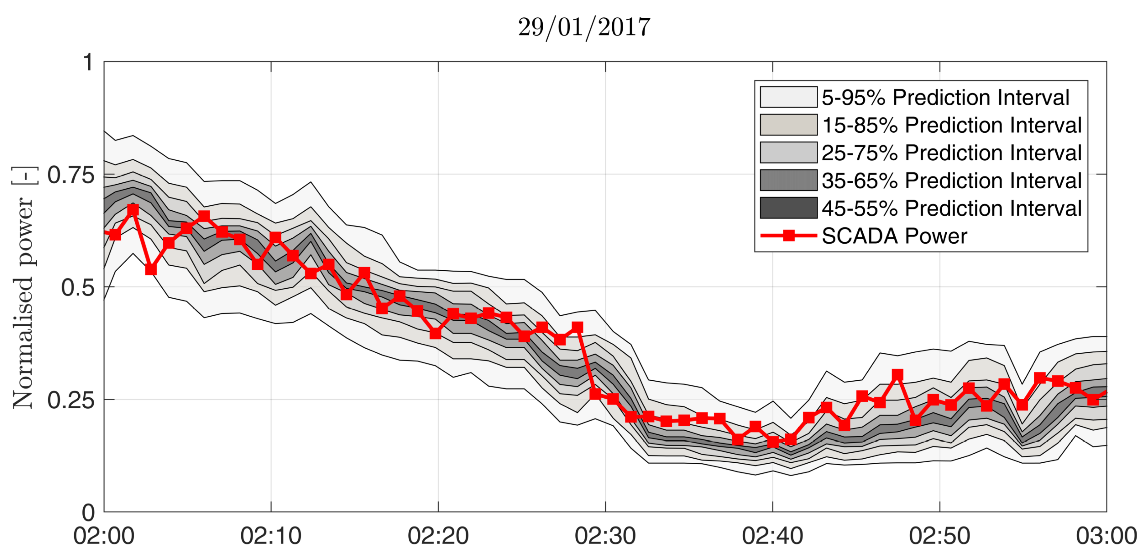Figure 10 depicts a one-hour episode of the RF model of power for $WT3$ together with the observed power. As stated before, the forecast is generated every minute. A strong decrease of power during the first half hour of the event is shown, which is properly captured by the RF model. To assess all wind turbines equally, we reduce the number of samples to the periods where all wind turbines operate simultaneously (Table 1, lower row) and there are available forecasts (T = 343). In general, RF is more skillful than persistence, except for $WT1$.

When assessing calibration of predictive densities, the use of quantile–quantile reliability diagrams is recommended [41]. In a reliable probabilistic forecast model, x% of the observations should be below the xth percentile of the distributions, as in the diagonals of Figure 11. However, the sample size of the evaluated forecast strongly influences the reliability of the diagrams, and even if the forecasts are highly reliable, a reduced sample size can lead to a reliability diagram deviating from the diagonal. Therefore, 95% consistency bars are generated following the work of Bröcker and Smith [42]. Here, we evaluate the predictions in quantile intervals with steps of 5%. Climatology is not represented since it has perfect reliability when evaluated over the whole sample set, as predictive densities are directly derived from the observations.

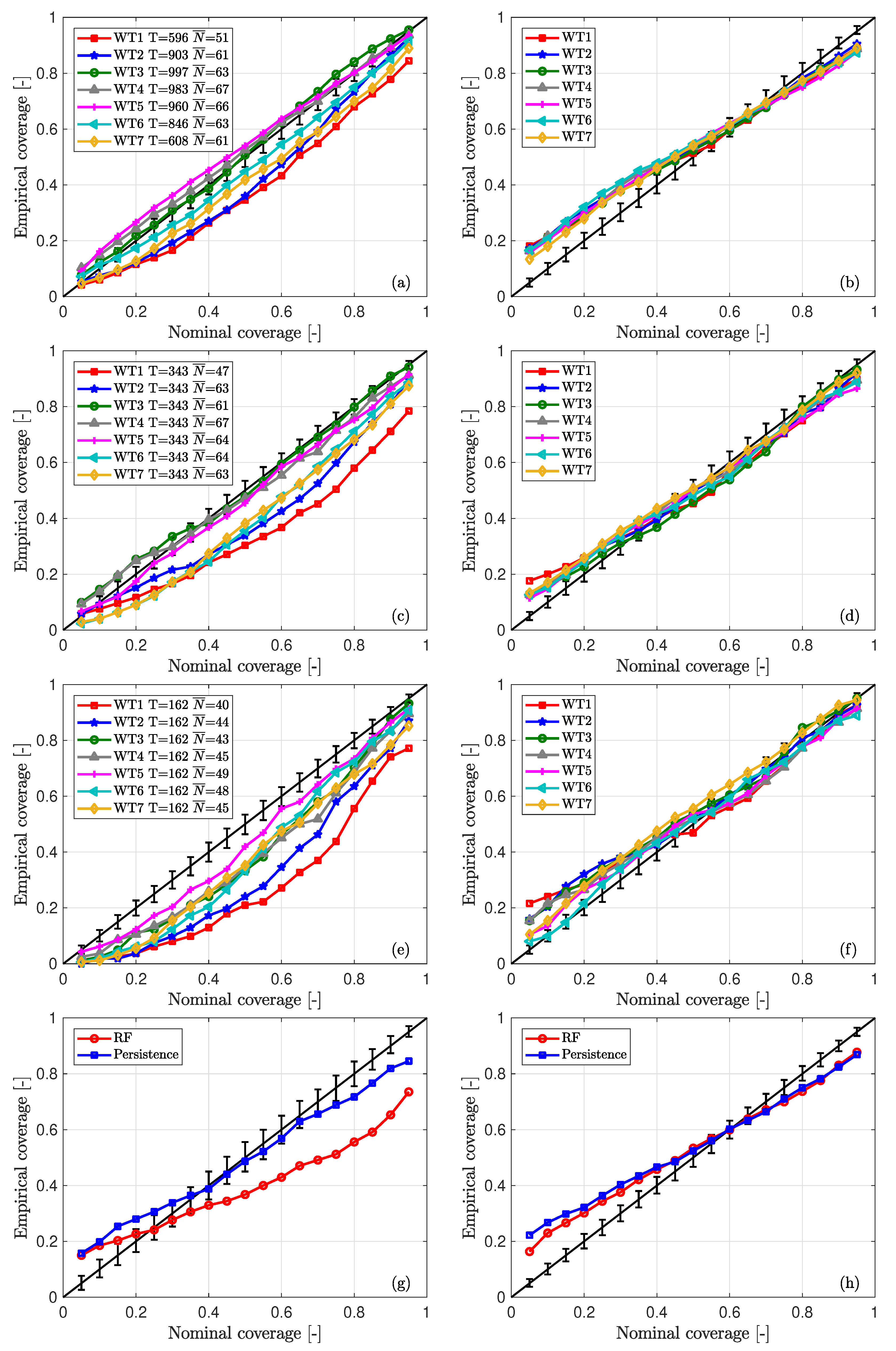
Figure 11a illustrates the reliability diagram of the RF model for the seven wind turbines of the first row, considering all available measurements. In the legend, the number of periods evaluated for each wind turbine (T), along with the average number of DD wind field vectors used to derive the predictive densities ($\overline{N}$) is included. Wind turbines $WT3$, $WT4$ and $WT5$ show reliable forecasts, as their reliability diagrams are close to the diagonal and most of the evaluated quantiles fall within the confidence intervals. In Figure 11b, the reliability diagram of the seven wind turbines when forecasted with the persistence method is depicted. The persistence method shows a poor calibration since nearly 18% of the observations are below the 5% quantile, while only around 88% of the observations are below the 95% quantile. In addition, over half of the evaluated quantiles do not lie within the 95% intervals around the diagonal. Contrary to the RF method, little differences are found among the reliability of the seven wind turbines. Figure 11c,d illustrate the previous reliability diagrams but limiting the analysis to simultaneous periods. In the case of the RF model, $WT1$, $WT2$, $WT6$ and $WT7$ also highly deviate from the diagonal, while the central wind turbines show a consistently reliable performance. Again, little differences are found among the seven wind turbines for the persistence model, but a generally worse performance than the the RF model is distinguished for wind turbines $WT3$, $WT4$ and $WT5$.

These results allow us to infer that the reliability of the RF model is not directly affected by the reduced sample size of the evaluation set, but by the individual position of each wind turbine within the radar measurement domain. Indeed, the fact that $WT3$, $WT4$ and $WT5$ lie closer to the center of the radar image and have a larger area from which the wind vectors can be advected to the target wind turbine, results in a more skillful forecast for those wind turbines. This hypothesis is further investigated in the following subsection by limiting the spatial availability of the radar measurements.

4.2. Analysis on Limited Radar Availability

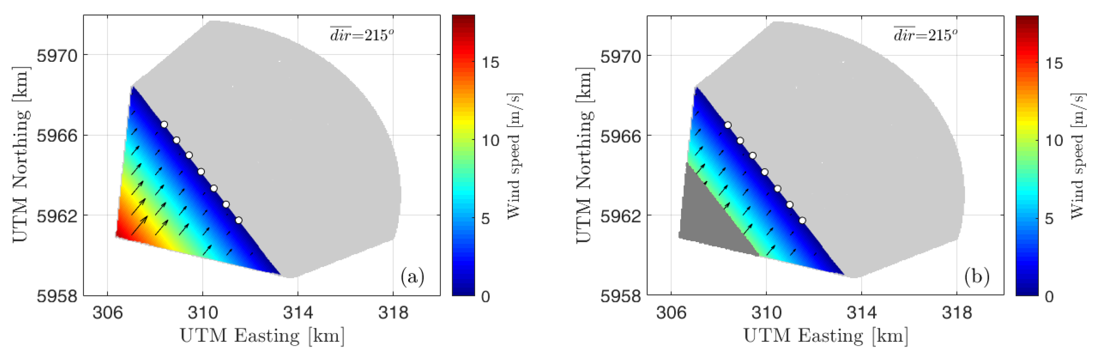
Here, we conduct a further analysis of the probabilistic performance of the RF model for individual wind turbines, relating the spatial coverage of the radar scan to the inflow area of each wind turbine, where potential wind vectors can originate from.

Figure 12a depicts the wind speeds that could be observed by each wind turbine for a given south–south westerly direction, setting a forecasting horizon of five minutes. As it can be seen, the turbines in the center have an advantageous positioning within the radar scan, as the range of wind speeds that can be observed is larger than that of the outer wind turbines. To test the hypothesis that the position of the wind turbines with respect to the radar domain influences the reliability of the RF model, we conduct a further experiment. Data measured in the furthest section of the radar domain (dark gray are in Figure 12b) are discarded, as if the radars no longer measure that section.

The results for the probabilistic forecast are presented in

Table 2. Average continous ranked probability score (CRPS) of five-minute ahead forecasts of power for the seven wind turbines evaluated, in the case of a reduced radar availability (Figure 12b). Results (in % of the nominal capacity ($P_n$)) are shown for the remote sensing-based forecasting (RF) model, persistence and climatology benchmarks.

		$\mathit{WT}\mathbf{1}$	$\mathit{WT}\mathbf{2}$	$\mathit{WT}\mathbf{3}$	$\mathit{WT}\mathbf{4}$	$\mathit{WT}\mathbf{5}$	$\mathit{WT}\mathbf{6}$	$\mathit{WT}\mathbf{7}$
	T	162	162	162	162	162	162	162
	RF	5.09	3.75	3.45	4.25	3.91	3.49	3.99
CRPS [%]	Persistence	4.58	4.56	4.41	4.84	4.10	3.75	4.36
	Climatology	20.73	19.86	19.19	18.83	18.51	17.97	17.57

. Regarding the overall skill, the RF performs better than the benchmarks in all WTs except for $WT1$.

As for the calibration, Figure 11e shows the reliability diagram for the RF model, in the case of having a reduced radar spatial coverage. It can be seen that the reliability of wind turbines $WT3$, $WT4$ and $WT5$ strongly decreases when the radar available area is reduced. Furthermore, the reliability of the other wind turbines is almost unchanged. For persistence (Figure 11f), small differences are found among the wind turbines, but here the reduced sample size analysed (T = 162) also influences the calibration.

4.2.1. Wind Farm Row Aggregated Power Output

In this section, we evaluate the probabilistic forecast for the average aggregated power produced by the wind turbines. The aggregated power is calculated adding the power distributions of the wind turbines using again a bootstrap resampling technique. Here, we evaluate the aggregated power of the seven wind turbines (${\overline{P}}_{17}$) and the aggregation of the central wind turbines $WT3$ to $WT5$ (${\overline{P}}_{35}$). The average aggregated power for both cases is given below:

$${\overline{P}}_{17}=\frac{1}{7}\sum _{i=1}^7{P}_i\mathrm{and}{\overline{P}}_{35}=\frac{1}{3}\sum _{i=3}^5{P}_i.$$

(5)

Table 3. Average continous ranked probability score (CRPS), in % of the nominal capacity ($P_n$), for the five-minute ahead predictive densities of aggregated power of different sets of wind turbines. T indicates the sample size evaluated. Minimum values are shown in bold. Results are shown for the remote sensing-based forecasting (RF) model, persistence and climatology benchmarks.

		${\overline{\mathit{P}}}_{\mathbf{17}}$	${\overline{\mathit{P}}}_{\mathbf{35}}$
	T	340	902
	RF	4.19	3.87
CRPS [%]	Persistence	4.98	4.75
	Climatology	15.51	16.61

summarizes the results for the aggregation of the wind turbines $WT1$ to $WT7$ (${\overline{P}}_{17}$) and $WT3$ to $WT5$ (${\overline{P}}_{35}$). The RF model has the lowest CRPS when evaluating the aggregation in both cases.

Regarding reliability, the quantile–quantile reliability diagram of the RF model for ${\overline{P}}_{17}$ (Figure 11g) performs worse than the probabilistic extension of persistence. We attribute this results to the fact that there are large differences in the RF model for the seven wind turbines, as mentioned in Section 4.1.1. As $WT3$, $WT4$ and $WT5$ are located at a more favourable position in the radar scanned area, in terms of inflow measurements coverage for the prevailing south–southwesterly direction, we further evaluate the aggregation of power considering only those wind turbines. Figure 11h depicts the reliability diagram of the RF model for the aggregation of wind turbines $WT3$ to $WT5$. In this case, the RF model is better calibrated than that of the ${\overline{P}}_{17}$ case, and presents even a better performance than persistence. However, in all cases reliability diagrams fall outside of the confidence intervals and it is clear that further work needs to be conducted to increase the reliability of the RF forecasts. However, given that spatio-temporal correlations among wind turbines can not be neglected, a different method to generate confidence intervals should be considered to draw more solid conclusions about the reliability of the evaluated methods for aggregated wind power.

4.3. Evaluation of Single Point Predictions

In this section, we evaluate the performance of single point or deterministic forecasts of wind power for individual and aggregated wind turbines and compare them with the persistence and climatology benchmarks. As stated before, the classical persistence reference forecast is a naive predictor, since it assumes that there is no change in the predicted variable. For climatology, we use the mean of the climatology distributions previously defined. Given that our target evaluation score is the RMSE of the produced power, we use the mean of the predictive density as the single point forecast.

4.3.1. Individual Wind Turbine Power

Table 4. Normalised root-mean-square-error (NRMSE), in % of the nominal capacity ($P_n$), of the five-minute ahead forecasts for the seven turbines of the first row. T indicates the number of periods evaluated. Minimum values are shown in bold. Results are shown for the remote sensing-based forecasting (RF) model, persistence and climatology benchmarks.

		$\mathit{WT}\mathbf{1}$	$\mathit{WT}\mathbf{2}$	$\mathit{WT}\mathbf{3}$	$\mathit{WT}\mathbf{4}$	$\mathit{WT}\mathbf{5}$	$\mathit{WT}\mathbf{6}$	$\mathit{WT}\mathbf{7}$
	T	596	903	997	983	960	846	608
	RF	10.06	7.90	7.70	8.93	8.50	8.16	9.06
NRMSE [%]	Persistence	9.40	8.54	8.68	8.89	8.81	8.49	8.80
	Climatology	31.34	30.39	30.13	29.84	29.66	29.49	29.19

compares the normalised root-mean-square error (NRMSE) of the five-minute ahead power predictions based on the RF model with persistence and climatology for the first row of wind turbines. The metric is normalised with the nominal power of the wind turbines. We show the results considering all periods available for each wind turbine. In four of the seven wind turbines, the NRMSE of the RF model is lower than that of the persistence method. For $WT1$ and $WT7$, persistence is better. For $WT4$, small differences between RF and persistence are found.

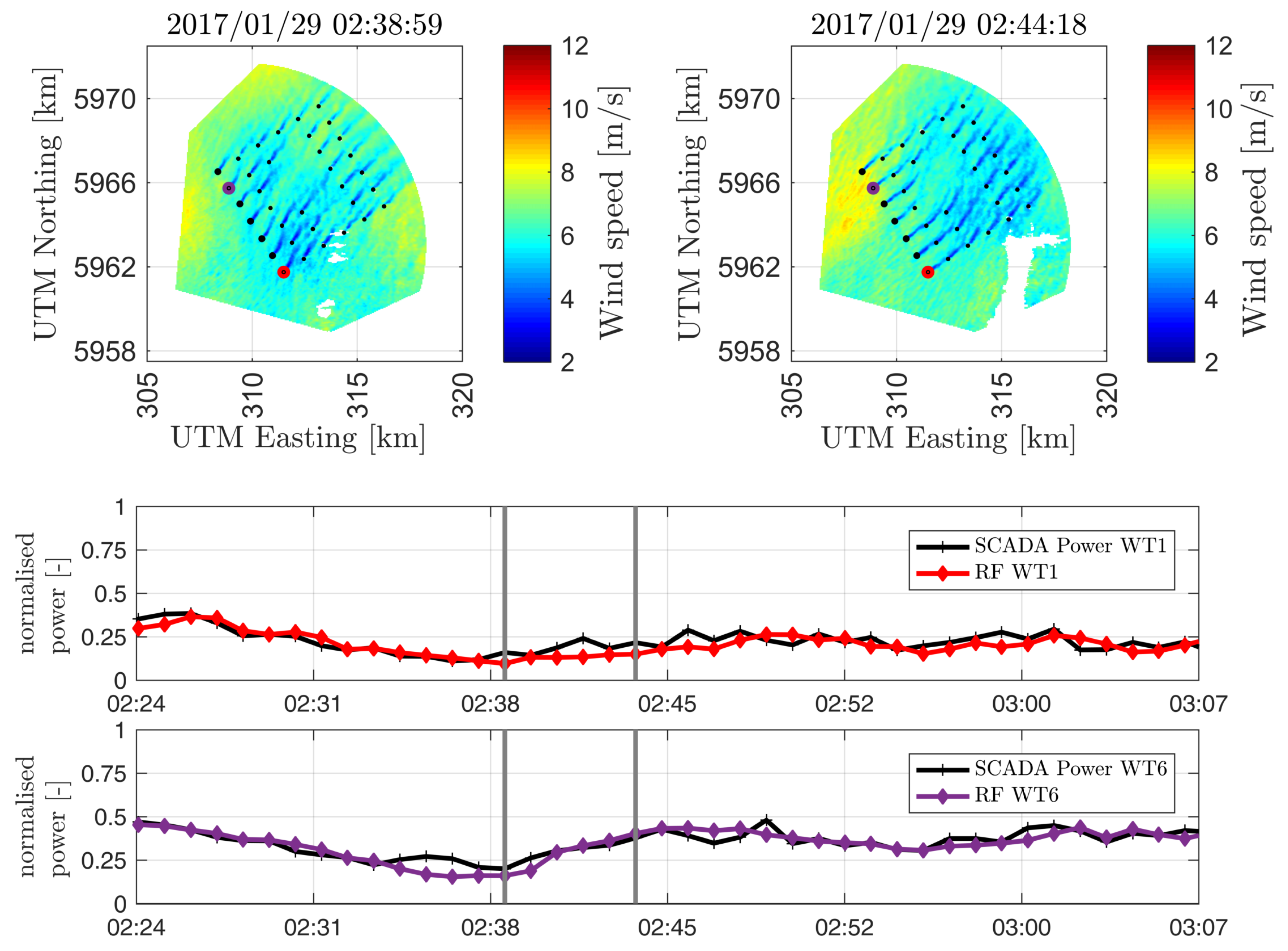
The way the RF model is able to anticipate strong variations of wind power, given by sudden changes in the flow can be clearly illustrated by exploring some interesting events. Figure 13 shows an episode of nearly 45 min of observed and predicted power for the wind turbines $WT1$ and $WT6$ together with the radar images at two time instants. On the left scan, a relatively homogeneous wind field is approaching the wind turbines in the first row, with slightly lower wind speeds in front of $WT1$ and $WT2$. Only five minutes later, higher wind speeds are experienced close to wind turbines $WT6$ and $WT7$, where two elongated streaks hit those wind turbines. This second period can be clearly identified in the time series at the bottom of Figure 13, where $WT6$ produces nearly double the power than $WT1$. The upcoming coherent structures can be observed in the top left image, in front of $WT6$. This episode highlights the importance of using observations for very short-term forecasting. A naive model such as persistence will predict the arrival of the increase in power for $WT6$ with a delay of five minutes.

In

Table 5. Normalised root-mean-square-error (NRMSE), in % of the nominal capacity ($P_n$), of five-minute ahead forecasts for the seven turbines of the first row, for the case of a reduced radar availability (Figure 12b). Results are shown for the remote sensing-based forecasting (RF) model, persistence and climatology benchmarks.

		$\mathit{WT}\mathbf{1}$	$\mathit{WT}\mathbf{2}$	$\mathit{WT}\mathbf{3}$	$\mathit{WT}\mathbf{4}$	$\mathit{WT}\mathbf{5}$	$\mathit{WT}\mathbf{6}$	$\mathit{WT}\mathbf{7}$
	T	162	162	162	162	162	162	162
	RF	10.09	7.35	6.83	8.89	8.01	7.09	8.01
NRMSE [%]	Persistence	8.02	7.89	7.48	8.74	7.86	6.93	8.56
	Climatology	35.49	34.15	33.08	32.51	32.04	31.00	30.51

, the results for the single point prediction, in the case of having a reduced radar availability are also listed. In this case, the limited radar domain spatial availability results in the RF model performing worse than in the case of having a full spatial radar availability.

4.3.2. Wind Farm Row Aggregated Power Output

Table 6. Normalised root-mean-square-error (NRMSE), in % of the nominal capacity ($P_n$), for five-minute ahead forecasts of average aggregated power. Results are shown for the remote sensing-based forecasting (RF) model, persistence and climatology benchmarks.

		${\overline{\mathit{P}}}_{\mathbf{17}}$	${\overline{\mathit{P}}}_{\mathbf{35}}$
	T	340	902
	RF	8.02	8.19
NRMSE [%]	Persistence	8.50	8.22
	Climatology	26.24	28.88

comprises the NRMSE for the case of aggregated power. The RF model exhibits the lowest NRMSE compared to climatology and persistence for both aggregated cases, ${\overline{P}}_{17}$ and ${\overline{P}}_{35}$. In the case of the aggregation of wind turbines $WT3$ to $WT5$, persistence is also a competitive model.

5. Discussion

In the current section, we discuss further uses of Doppler radar observations for wind power very short-term forecasting and address the limitations found in our proposed methodology.

5.1. On Further Use of Doppler Radar Measurements for Wind Power Forecasting

Doppler radars, like the ones used in the BEACon project, can measure up to 32 km, covering an area of more than 100 km${}^2$, which is in line with the size of modern offshore wind farms. Radar measurements covering the whole wind farm, such as the ones presented here, are very valuable to understand the turbine-to-turbine interaction. However, when it comes to forecasting wind power, the radars’ spatial coverage strongly influences the predictions. In the present case, an unfavourable scan geometry, with respect to the inflow area upstream of the outer wind turbines in the first row, resulted in degraded power predictions compared to the wind turbines positioned in the centre.

Therefore, an operational wind power forecasting system based on Doppler radar measurements should be configured with the aim of covering a sufficiently wide upstream area. As wake effects will influence the performance of downstream wind turbines, predictions of time series of the accumulated power of a whole wind farm are not straightforward. Both the power of the individual wind turbines, as well as the propagation of transient wind fields inside the wind farm, will strongly depend on the local dynamics and inhomogeneity of the wind farm flow. Further investigations are required to establish a suitable forecasting methodology. One approach might be to limit wind speed forecast to the first row of wind turbines (according to the prevailing wind direction). Additionally, turbine-to-turbine predictions of wind power accounting for wake losses could be used to predict the whole wind farm power generation.

One example time series demonstrated the ability of the radars to predict coherent structures affecting “locally” the power of individual wind turbines, which is beyond the current capabilities of commonly-used statistical methods for very short-term predictions. In a similar manner, it should be possible to probabilistically describe the effect of strong and fast changes in wind speed or direction, which cause wind power ramp events. Those crucial situations require risk-based decisions to be made, and there lies the importance of using a probabilistic approach. Given the current limitations of forecasting ramp events with NWP [43] and statistical [44] methods, radars could serve as a tool for detecting those extreme events. The maximal range of the BEACon radars (32 km) could detect a strong weather front of high wind speed (20 m/s) and give enough time for end-users to react.

As Doppler radars measure with a high temporal and spatial resolution, tracking techniques could also be applied to determine the vorticity and diffusion of identified patterns, extending the available information to determine the future position of the wind field vectors or wind coherent structures. Additionally, vertical information from the radars could be used to better describe gusts and lulls. Following this line, radar measurements at multiple heights could be used to derive a rotor equivalent wind speed which extends to the whole rotor plane and, unlike the hub height wind speed, accounts for the shear.

5.2. On Extension of the Forecasting Horizon

Due to the setup of the experiment and the prevailing south-westerly direction of the analysed data set, the wind field could only be evaluated over a relatively short distance of 5 km limiting the prediction horizon to five minutes. However, the long measurement range and the high spatial and temporal resolution of the used Doppler radars of up to 32 km should enable longer lead times on the order of 10 to 15 min as well. In principle, the proposed methodology should be capable of such horizons.

The proposed methodology is based on the advection of the wind field vectors with their respective motion, i.e., the persistence of their trajectories. Despite the promising results presented in this work, the question remains whether such assumption could be considered for longer horizons, increased turbulence, different types of stratifications, ramp events, strong veering or complex terrains. Based on our understanding, using a probabilistic approach should be able to include some (if not all) related uncertainties.

5.3. On Data Quality

One limitation of remote sensing prediction models is the uncertainty associated with the observations. Forecasting wind power based on wind speed observations introduces a new source of uncertainty. In this work, we overcome this problem by using a power curve based on the local dual-Doppler observations and the observed SCADA data that could, systematically, remove any bias introduced from the different type of measurements used to derive power curves. In a similar way, hybrid models using the radar observations and correcting for time-dependent errors should be explored.

Finally, reduced availability of data is a limitation inherent in remote sensing measurements, as the quality of those measurements highly depends on the meteorological conditions. In this regard, solutions for using Doppler radars in non-optimal meteorological situations need to be explored. Emphasis should be put on using data assimilation techniques, where observations are fed into statistical methods or NWP models, as such methods have shown to be improved when combined with real observations [45,46].

6. Conclusions

This paper investigated the use of DD radar observations to derive deterministic and probabilistic forecasts of wind power in a very short-term horizon of five minutes. An advection Lagrangian persistence technique was introduced to determine the predictive densities of rotor wind speed. In a case study, the proposed methodology was used to forecast the power generated by seven wind turbines in the North Sea, during free-flow conditions. The five-minute ahead predicted mean wind speeds corrected for induction effects showed a high degree of correlation with the observed DD wind speeds 2.5D upstream of the wind turbines. The predicted wind speeds densities were transformed into power densities by using a probabilistic power curve. We compared the proposed probabilistic forecast of wind power with the benchmarks persistence and climatology. Our results have shown the superiority of the remote sensing-based forecasting model regarding overall forecasting skill. However, a large spatial radar coverage of the inflow of a wind turbine is necessary to generate reliable density forecasts. The results have also proven that upstream remote sensing observations are especially crucial to detect strong changes in wind power, as shown in an example of a fast and strong predicted increase in power. Based on our results, a DD radar-based forecast might have a positive impact on the integration of offshore wind power into the grid.

Future works should be devoted to forecast the power produced of the whole wind farm, including wake effects, and to detect ramp events where the wind speed and direction changes rapidly. In addition, it is considered promising to further analyse DD radar measurements to enable the extension of the forecasting horizon and to improve the wind power predictions for different meteorological conditions.