Identifying Tree-Related Microhabitats in TLS Point Clouds Using Machine Learning


1
Swiss National Forest Inventory, Department of Forest Resources and Management, Swiss Federal Institute for Forest, Snow and Landscape Research WSL, Zürcherstrasse 111, 8903 Birmensdorf, Switzerland
2
Department of Landscape Dynamics, Swiss Federal Institute for Forest, Snow and Landscape Research WSL, Zürcherstrasse 111, 8903 Birmensdorf, Switzerland
*
Author to whom correspondence should be addressed.
Remote Sens. 2018, 10(11), 1735; https://0-doi-org.brum.beds.ac.uk/10.3390/rs10111735
Submission received: 27 September 2018
/
Revised: 29 October 2018
/
Accepted: 31 October 2018
/
Published: 3 November 2018
(This article belongs to the Special Issue 3D Point Clouds in Forests)
Abstract
:Tree-related microhabitats (TreMs) play an important role in maintaining forest biodiversity and have recently received more attention in ecosystem conservation, forest management and research. However, TreMs have until now only been assessed by experts during field surveys, which are time-consuming and difficult to reproduce. In this study, we evaluate the potential of close-range terrestrial laser scanning (TLS) for semi-automated identification of different TreMs (bark, bark pockets, cavities, fungi, ivy and mosses) in dense TLS point clouds using machine learning algorithms, including deep learning. To classify the TreMs, we applied: (1) the Random Forest (RF) classifier, incorporating frequently used local geometric features and two additional self-developed orientation features, and (2) a deep Convolutional Neural Network (CNN) trained using rasterized multiview orthographic projections (MVOPs) containing top view, front view and side view of the point’s local 3D neighborhood. The results confirmed that using local geometric features is beneficial for identifying the six groups of TreMs in dense tree-stem point clouds, but the rasterized MVOPs are even more suitable. Whereas the overall accuracy of the RF was 70%, that of the deep CNN was substantially higher (83%). This study reveals that close-range TLS is promising for the semi-automated identification of TreMs for forest monitoring purposes, in particular when applying deep learning techniques.
1. Introduction
Monitoring of forest biodiversity is a key issue in the context of sustainable forest management [1]. Multi-purpose forests need to provide habitats for animals and plants to fulfill their ecological function, as well as performing economic and social functions. Stem structures, such as cavities, epiphytes and other tree-related microhabitats (TreMs), serve as habitats at the tree level and are existential for a wide range of insects, birds and mammal species during their life cycles [2,3]. The abundance and diversity of TreMs affect the ecological value of a tree [4,5]. TreMs are thus important indicators of forest biodiversity and have recently received more attention in ecosystem conservation, forest management and research [6].
The abundance and diversity of TreMs can be roughly predicted using tree characteristics, such as tree species, vitality status and diameter at breast height (DBH) [7,8,9]. More precise estimations of TreMs could be obtained by experts during field surveys, but their reproducibility remains challenging, since it is strongly affected by the observers [7,10,11]. Standardization of TreM assessment, as proposed by [12], should increase the reproducibility of TreM surveys, but such surveys are still very time-consuming and preferably conducted by at least two experts [11]. TreM assessment in the field has so far been mostly conducted in small forest areas and rarely in national forest inventories [13]. In the Swiss National Forest Inventory (NFI), TreMs have been partially recorded in the field survey for 35 years [10]. According to the information needs of NFI stakeholders, numerous TreMs have been added to the field data catalogue of the ongoing fifth Swiss NFI [7]. Thus, reproducible and efficient methods for assessing TreMs are therefore needed for future NFI surveys.
Recent developments in terrestrial laser scanning (TLS) allow for efficient mapping of object surfaces in dense 3D point clouds. In contrast to other 3D remote sensing measurement techniques (e.g., air- and UAV-borne LiDAR and stereo images), TLS allows capturing precisely very detailed 3D information (in the millimeter range) below the canopy cover, i.e., on tree stems and understory. Over the past decade, the potential of TLS has been actively tested to complement or, in the future, even replace extensive field surveys for forest monitoring, including for conventional NFIs [14,15,16,17]. Researchers have already made big advances in defining optimal scanning designs for inventory plots [18] and for deriving a wide range of plot-level and tree-level characteristics, such as tree-stem detection [19] and modeling [20,21,22], tree species recognition [23,24], DBH extraction [25], determination of leaf area distribution [26], volume estimation [27], detection of clear wood content [28] and wood defects [29], assessment of timber quality and timber assortments [30]. TLS 3D point clouds have also successfully been used to derive forest structural information to evaluate the suitability of a forest stand as a habitat for animals, e.g., bats [31] or birds [32]. Whereas TLS 3D point clouds have already been partly used to analyze stem structures in terms of wood quality [28,29], they have not yet been used for detecting and quantifying TreMs.
Object detection in 3D point clouds has successfully been performed by fitting 3D geometric primitives [22,33], filtering of point clouds using logical operators [19] or semantic labeling applying machine learning techniques [34,35]. Machine learning algorithms have experienced great success, in particular in identifying objects with irregular structures, e.g., natural objects. In the remote sensing of the environment, the best classification results have most often been obtained when using Random Forest (RF) and Support Vector Machine (SVM), mostly in combination with hand-engineered features (e.g., [36]). Meanwhile, RF has become a favored classification approach for semantic labeling of both image data and point clouds, because of its high performance, its robustness to overfitting and nonlinearities of predictors, its ability to handle high-dimensional data, and its computational efficiency [35,37].
However, the performance of any classifier strongly depends on the features, which need to be sufficiently discriminative. For 3D point clouds, a wide range of local 3D descriptors that encode the geometric properties of the local neighborhood of a 3D point have been proposed in the literature [38]. These geometric features which are derived based on the covariance tensor of a point’s local neighborhood, are popular in LiDAR data processing, due to their efficient computation and relatively easy interpretation. They have been used, for example, to label unstructured TLS point clouds [34,35,39], detect contours [39], filter the TLS point clouds collected in a forest environment [20,40], and discriminate foliar and woody materials in a forest [41]. However, it is challenging to find an optimal neighborhood for calculating the local geometric features, since this is affected by the local point density and the geometric characteristics of the object of interest. The neighborhood of a point is thus often chosen heuristically [39] or calculated on multiple scales [34,35].
Object detection greatly benefits from learning of deep representatives. Recent developments in computational hardware and the possibility of greatly speeding up the training time of deep neural networks with parallel computation using Graphical Processing Units (GPUs) have initiated a new era when deep learning has been the subject of great interest. Convolutional Neural Networks (CNNs), which learn deep representations directly from the data, have meanwhile become a state-of-the-art approach in both 2D image classification and segmentation [42,43]. Although CNNs were primarily designed for 2D data, they have already been successfully applied for semantic labeling of 3D point clouds using the 3D point cloud information directly [44,45,46] or their 2D representations, i.e., 2D images [47,48]. While learning, CNNs generate class-specific high-level features (representations) from low-level input information. The impressive results achieved with CNNs can be improved even further by integrating contextual information using Conditional Random Fields or Recurrent Neural Networks [49]. Moreover, features generated by CNNs can be used to train a classical machine learning approach, such as SVM [50].
In this study, we addressed the potential of TLS for semi-automated identification of TreMs, since expert field assessment is difficult to reproduce. We trained both a classical machine learning approach involving hand-engineered features (RF) and a deep neural network based on learned features (CNN) to perform point-wise semantic labeling of TLS point clouds, with the goal to identify six groups of stem structures associated with TreMs. Therefore, in this paper, we conducted research to: (1) evaluate the suitability of the RF trained on commonly used local geometric features for TreM identification; (2) develop two additional local geometric features and illustrate their contributions to the RF performance; (3) evaluate the potential of a deep CNN for TreM identification from 3D point clouds; (4) propose an approach to generating 2D input data for a CNN based on 3D point cloud information; and (5) discuss the suitability of TLS point clouds for TreM identification.
2. Materials and Methods
2.1. Data Acquisition
In this study, we focused on identifying TreMs on beech (Fagus sylvatica L.). In Switzerland, forest biodiversity and the ecological needs for TreMs are greatest in the lowlands, e.g., in the colline and submontane zones, where beech is naturally dominant on most sites [51] and forests are often intensively managed. Beech is thought to have considerable potential for accumulating TreMs [6,8].
A FARO Focus 3D S120 laser scanner (FARO Technologies Inc., Lake Mary, FL, USA) was used to collect data. It is a high-speed phase-shift scanning device with a high-precision measurement capability and a small footprint (Table 1). TLS data were acquired in several forest reserves and managed forests across Switzerland. Scanning design was primarily developed to scan one single habitat tree. The habitat trees were, thus, scanned from six different positions regularly distributed around the tree. The angular resolution was set to 0.018°, which corresponded to a point spacing of 3 mm at a 10 m distance from the scanner. This allowed us to obtain the data with a very high point density. Intensity and RGB values were acquired as well (Table 2). In total, 29 beech habitat trees were scanned.
2.2. Field Assessment of TreMs
In order to get a sufficient number of each type of TreM without excessive effort, we had to focus on these types that are of main interest [12], as well as relatively frequent (own field experience, [52]) and visible from the ground. According to the TreMs assessment in the fourth Swiss NFI, around 80% of TreMs are located on the tree stem and thus contribute the most to the ecological value of a tree. This is why we focused on tree stems. We did not consider the TreMs in tree crowns due to high occlusion rates in the TLS data. We recorded all TreMs located on the stem of a scanned habitat tree below Hmax, where Hmax corresponded to 10 m or the height of the first branch. The TreMs addressed in this study and the thresholds for their inclusion are listed in Table 3. The thresholds were chosen to correspond or being lower than these in the field manual of the current fifth Swiss NFI [53].
For countable TreMs, such as bark pockets, cracks or fungi, located at a height of ≤3.5 m on the tree stem, we measured their positions and dimensions. For those located at a height above 3.5 m, the dimensions were estimated. For uncountable TreMs, such as ivy, mosses, lichens or missing bark, we estimated their coverage (in percent) in the lower (0–2 m), middle (2–4 m), and upper (4–Hmax m) parts of the tree stem. To specify the location of a TreM, the azimuth (gon), vertical angle (grad) and horizontal distance (m) were measured. Additionally, detailed photos were taken from each scanner position along the stem of the scanned habitat tree, using a conventional digital camera with a high resolution.
2.3. Point Cloud Pre-Processing
First, the scans collected in the field were accurately co-registered using reference targets in the FARO Scene software (version 5.4, FARO Technologies Inc., Lake Mary, FL, USA). Second, the stem part of interest in this study up to 10 m or to the height of the first branch was then manually delineated from the initial point cloud using CloudCompare software [54]. Third, tree-stem point clouds were thinned out using a 3 mm voxel grid, so that only the point located next to the voxel center remained. Fourth, the Statistical Outlier Removal (SOR) filter was applied to reduce the noise produced by the sensor. The SOR calculates the mean μ and standard deviation σ of distances from point pi to its k nearest neighbors. Points located beyond the threshold μ ± α ∙ σ are considered to be outliers and are removed [55]. In this study, we set k = 5 and α = 1.
2.4. Stem Axis Fitting
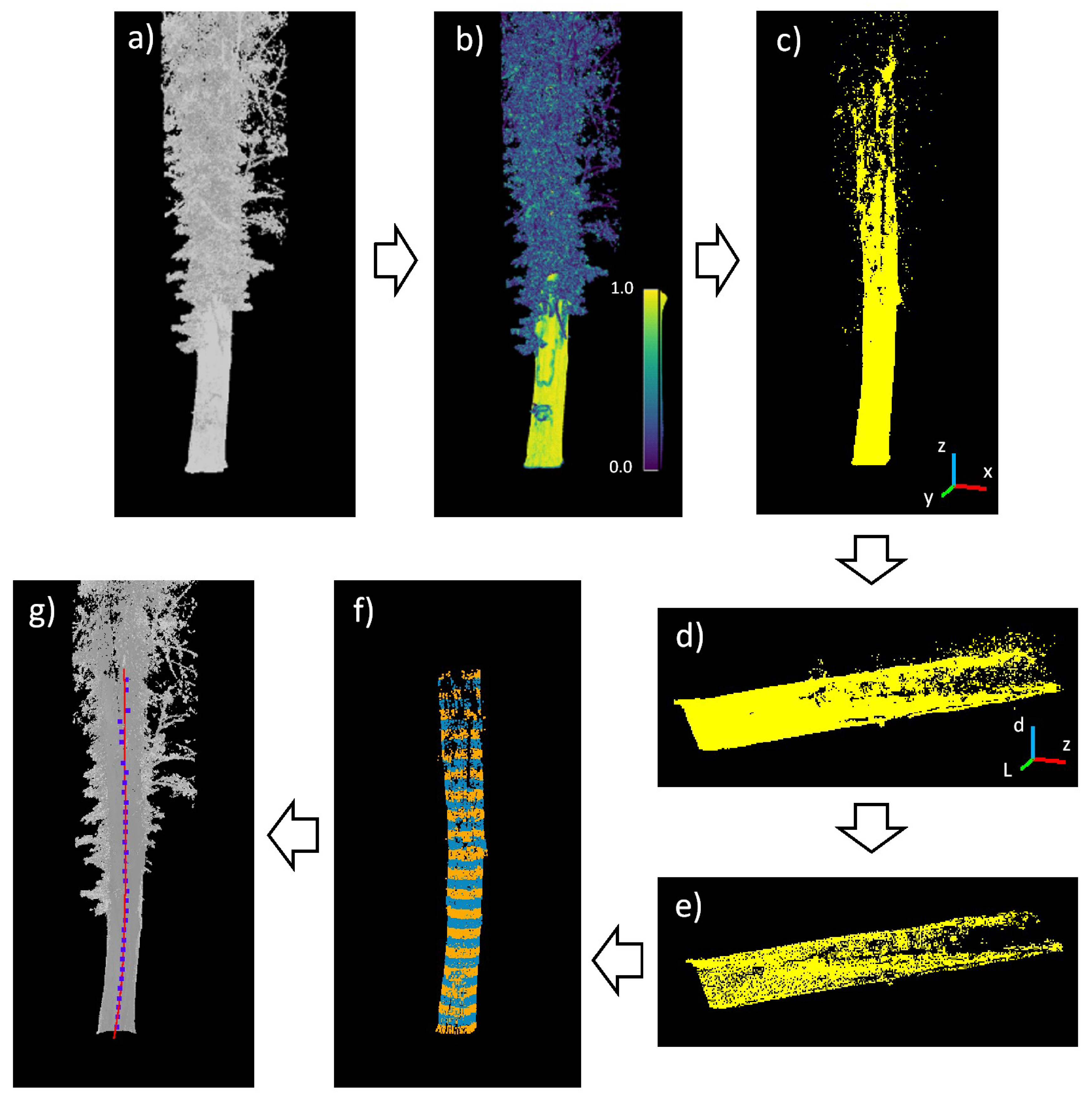
Since a tree stem is a cylindrical object, detecting its axis (centerline) is likely to be helpful when analyzing its surface. Various methods have been used to define stem axis, such as cylinder fitting [56] and normal accumulation [29]. It might be necessary to slightly adapt both of the methods prior to applying them to habitat trees, which are often characterized by rich tree stem structures. We therefore developed a method to define the tree stem axis of habitat trees. This method involves: (1) intensive pre-filtering of the tree stem in terms of reducing the structural variability on its surface, and (2) modeling a curve through the centers of the circles fitted into the stem cross-sections. This procedure consisted of several steps (Figure 1).
First, we used geometric information (xyz coordinates) of the tree-stem point cloud (Figure 1a) to calculate the planarity feature (Figure 1b; see the detailed description of feature extraction in Section 2.5.2.2). The planarity is associated with features that describe shape characteristics and is calculated based on eigenvalues of a 3D covariance matrix. In the case of 3D points, equally distributed on a squared plane, the planarity is expected to be equal to 1 and is below this value for the 3D points equally distributed on a rectangular plane with unequal sites (typically for edge regions). However, according to [57], the values of the planarity might deviate from the expected values. Thus, the tree stem was roughly extracted by removing non-flat regions in the tree-stem point cloud using the planarity. Since the stem of a habitat tree can have many edges, we retained all the points with a value above the threshold of 0.75 (Figure 1c). The planarity was also used by [20] to remove non-flat regions in TLS point clouds in their denoising and tree-stem modeling algorithm (threshold of 0.8). In the following step, we refined the tree-stem filtering by extracting the points located closest to the surface of the tree stem. For this, the xyz coordinates of the filtered tree-stem point cloud were transformed (“unrolled”) into Lzd coordinates using a cylinder modeled based on the point cloud (see Figure 1c and for more details, see [56]). The transformed point cloud was then divided into vertical columns using a regular 2D raster (based on Lz coordinates) with a window size of 3 cm. In each raster cell, only the point with the lowest d coordinate was retained (Figure 1e). The resulting point cloud was then converted back into xyz coordinates, and multiple circles were fitted along the tree stem. For this, the point cloud was divided into non-overlapping cross-sections which was 20 cm wide (Figure 1f). For each cross-section, a circle was fitted using the least squares method (outliers were removed). In the following step, the circles were analyzed to define extreme values in their diameters and remove those with diameters considered to be statistical outliers. We then fitted a curve through the centers of the remaining circles by training a multilayer perceptron (MLP) [58]. The MLP consisted of one hidden layer. The number of neurons in the hidden layer was tuned via grid search for each separate tree stem. The number of iterations, while training the MLP, also varied and depended on the length of the tree stem. For each additional 1 m of stem length, 100 more iterations were added. The gradient descent optimization algorithm and linear activation function were applied. The resulting root-mean-square errors (RMSEs) for effective and predicted circle centers revealed RMSEmin = 0.01 m, RMSEmax = 0.05 m, meanRMSE = 0.026 m and sdRMSE = 0.015 m. An example of a fitted stem axis is shown in Figure 1g.
The fitted stem axes were used for: (1) extracting orientation features for RF classification models (see details in Section 2.5.2.2), and (2) generating input data for CNNs (see details in Section 2.5.3.2).
2.5. Classification
Two different classification approaches were tested to identify TreMs in the tree-stem point clouds. First, a RF classifier was trained using two different sets of hand-engineered features. Second, a CNN was used for both extracting features and classification, and was trained with and without the input being augmented (Table 4).
2.5.1. Training Data Set
For the training data set, patches of 3D points belonging to a TreM were manually delineated from the tree-stem point clouds. The collected patches corresponded mostly to a complete object (e.g., a fungus or a bark pocket). For not countable (continuous) TreMs, such as mosses, lichen or ivy, parts of the tree stem covered with it were chosen for training. We also collected patches of bark only (without any TreMs). In total, 173 patches with varying numbers of points were collected. Since some of the TreMs are rare (e.g., cracks and woodpecker holes), we assigned them according to similarities in their geometric properties to the following six TreM groups: bark (including bark and exposed wood), bark pockets, cavities (including cracks, stem cavities and holes, woodpecker cavities and holes), fungi, ivy, and mosses (including mosses and lichens). For details about the training data set, see Table 5.
It is not necessary to use the complete training set to achieve an appropriative classification model (see e.g., [35]). Thus, we rebalanced our training set and reduced it to 10,000 training points per class, which were randomly selected from the initial data set. To evaluate how well the reduced training set represents the complete training set, we run ten RF classification models. For each RF model, a new training set was generated using random selection of 10,000 points per class. The performance of the RF models was evaluated using a 5-fold cross-validation procedure, which was repeated three times. The resulting mean overall accuracy was 75.5% and the standard deviation was 0.4%.
2.5.2. Random Forest
2.5.2.1. Classifier
RF is an ensemble classifier, consisting of a collection of randomized decision trees [59]. The high performance and robustness of RF were achieved by implementing bagging [60], a learning procedure designed to improve the stability and performance of weak machine learning algorithms. For RF, a large number of decision trees are trained on training sets generated from the original data set, using random sampling with replacement. While growing the trees, the user-defined number of predictors are randomly selected at each split. This multiple randomization procedure results in non-correlated trees being produced with high variance and low bias [61]. The final classification output is created by aggregating the predictions of all individual decision trees using majority voting.
Two parameters that need to be adjusted when training RF are the number of trees (ntree) and the number of predictors used at each split (mtry). According to [62,63], 500 trees are enough to stabilize the model. Our pre-tests confirmed this and showed that, in our case, using a higher number of trees does not affect the performance of the RF classification models. Thus, we set ntree to 500. The RF seems to be quite sensitive to the mtry parameter [36,62]. It is recommended to tune mtry for each separate case, since this parameter depends on the fraction of relevant predictors. If this is low, small values of mtry may result in a poor model performance since the chance that the relevant predictors will be selected at each split is low [61]. We trained RF using the train function of R package caret [64]. By default, this function tests three different options for mtry: the lowest, the highest and the mean value of both. The model with the lowest out-of-bag error was selected as the final model.
2.5.2.2. Local Geometric Features
To train RF, we derived a set of features from the geometric information of the TLS point cloud. The FARO Focus 3D S120 laser scanner captures geometric (xyz coordinates) and spectral information (RGB and intensity) of the surrounding objects. Since RGB values are very sensitive to the sun illumination and intensity values need to be corrected [65], only xyz coordinates from the acquired point clouds were used in this study.
A point in a 3D point cloud can be characterized by its closest neighborhood, from which a set of local 3D geometric features can be derived. Two different procedures are most commonly used to define the point’s local neighborhood: (1) a fixed-number nearest neighbors’ search [35,39] or (2) a fixed-radius nearest neighbors’ search [34]. For a point-wise multiclass classification problem, the choice of the point’s neighborhood might be crucial since, for different classes, the discriminative power of the 3D geometries may vary across scales, i.e., across the search radii or number of nearest neighbors. Two different procedures have been proposed for this: considering an optimal 3D neighborhood for each individual point [35] or deriving geometric features on different scales [34,39].
To train the RF classifier, for each point in the point cloud, a set of 3D geometric features (Table 6) was derived. We selected the point’s 3D neighborhood using a fixed-radius nearest neighbor search on multiple scales, i.e., the 3D neighborhood of a point was selected using a sphere with a radius corresponding to the scale parameter r. The scale parameter r varied from rmin = 1 cm to rmin = 5 cm with ∆r = 0.5 cm. For each scale, a set of eigenvalues (, , ) and of eigenvectors (, , ) were extracted based on a covariance tensor around the medoid of the neighborhood of the point pi (for details, see [39]). The derived eigenvalues were normalized by their sum, and then used to calculate a set of 3D shape features: linearity, planarity, sphericity, omnivariance, anisotropy, eigenentropy and surface variation [35,39]. Since the normalized eigenvalues already characterize the geometric properties of the point’s neighborhood regarding its variations along eigenvectors, we used the first and the second of them (, ) as discriminative variables as well.
To capture local changes in the directions of the stem surface relative to the stem axis, we developed two additional orientation features. These features were inspired by the verticality feature used by [39], which was calculated as an angular product between the vertical axis and the local normal , where of a point . The two orientation features used in this study correspond to: (1) the angular product between the normal of a point and a vector directed to the center of the tree stem , (2) the angular product between the orthogonal projection of the of a point and a vector directed to the center of the tree stem . The values of the orientation features varied between 0 (when and the vector directed to were parallel) and 1 (when they were perpendicular). The whole set of the local 3D geometric features used in this study is listed in Table 6. See Figure 2 for visualization of a feature.
2.5.3. Convolutional Neural Network
2.5.3.1. Convolutional Neural Network Architecture
CNNs (also known as ConvNets) belong to the family of feed-forward artificial neural networks and were first introduced by [66]. In contrast to other classification approaches based on previously extracted features, CNNs learn specific features directly from the data. A CNN usually has a multi-layered architecture, which is represented by various combinations of convolutional, pooling, dropout layers, and with one or several fully connected layers. Convolutional layers are core structures in a CNN. In a convolutional layer, feature maps will be generated from an input image using convolutional filters. Each unit (neuron) of the feature map is connected only to a small subregion of the input image. The output of each convolutional layer is passed through an activation function (e.g., tanh or ReLU). After each convolutional layer, a pooling layer is often incorporated into downsample the feature maps along their spatial dimensions. Each feature map is therefore divided into usually non-overlapping subregions, for which an arithmetic operation is then performed (e.g., averaging or considering the maximum value). Reducing the dimensionalities of the feature maps leads to training of a much lower number of weights and a more computationally efficient network. The pooling layer also has a regulating effect.
Another very effective way to prevent overfitting and increase the generalization of the neural network is to introduce dropout layers. A dropout layer is specified by a dropout rate p, which indicates the probability of a neuron being “dropped out”, i.e., the weights of the “dropped out” neuron are set to zero. Deactivated neurons might then be used in the next iteration. In CNNs, dropout is usually applied to fully connected layers [67], but is also effective for convolutional layers [68]. A CNN is finalized with one or several fully connected layers when all neurons are fully connected to all activations in the previous layer. The last fully connected layer generates the output of the CNN and, in the case of a classification, its number of neurons corresponds to the number of classes (for more details, see [69]).
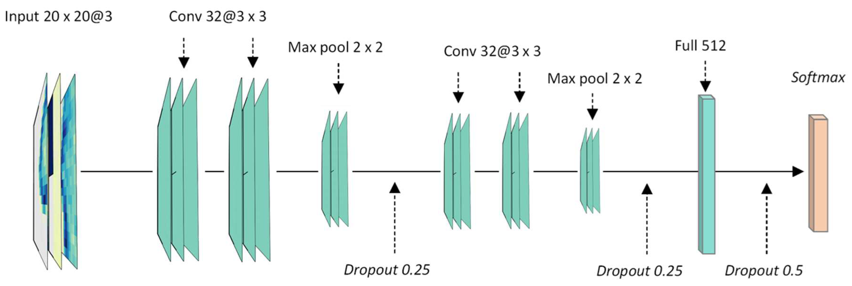
The input data for the CNNs in this study consisted of a stack of the three rasterized multiview orthographic projections (MVOPs) of the point’s local neighborhood (for details, see Section 2.5.3.2). The architecture of the CNN consisted of two pairs of convolutional layers, of which each was followed by a pooling and a dropout layer, and a fully connected layer with dropout (Figure 3). If several convolutional layers that follow each other are specified (e.g., [45,67]), more abstract representatives can be learned before implementing a destructive pooling layer and the performance of a neural network thus increase. We used an equal number of convolutional filters in all convolutional layers (32 filters with a window size of 3 × 3 and zero-padding). The output of each convolutional layer was passed through a ReLU. A pooling layer with a window size of 2 × 2 to calculate a maximum value (max-pooling) was introduced after every other convolutional layer. Dropout with a rate of 0.25 was applied to the resulting feature maps, which means that 25% of neurons were deactivated. The CNN was finalized with a fully connected layer consisting of 512 neurons and followed with a dropout layer with higher intensity (dropout rate = 0.5). The output of the neural network was generated using the softmax function. The CNN was trained for 50 epochs using a stochastic gradient decent with a batch size of 64 samples.
2.5.3.2. Rasterized Multiview Orthographic Projections (MVOPs)
Since a CNN requires input with array-like structures, 3D point clouds have to be processed accordingly, for example, voxelized [44,45]. Training a 3D CNN for very dense 3D point clouds might be computationally expensive since high numbers of weights need to be calculated. Additionally, such models might be sensitive to overfitting. We therefore developed a novel approach to generating input data for a CNN by converting the 3D information of a point cloud into a set of its 2D representations. Similar to hand-engineered geometric features, we characterized a 3D point in a point cloud through its local neighborhood. We hypothesized that TreMs, each represented by a typical shape, might also be distinguished by their rasterized MVOPs (top view, front view and side view) [70]. Using 2D representations, instead of 3D representations, of a point’s local neighborhood would mean much lower number of weights was trained and thus would increase the computational efficiency of our CNNs.
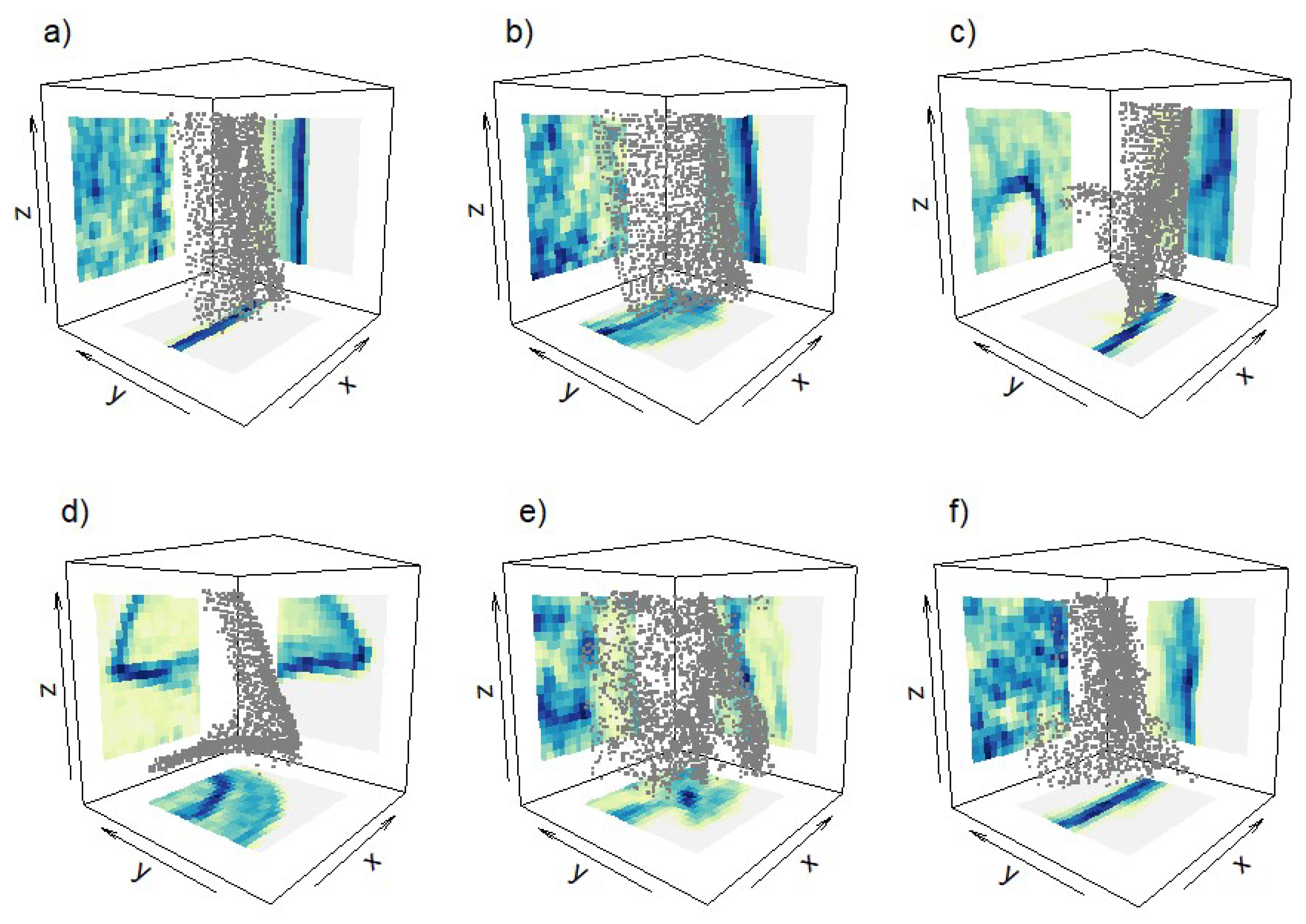
The rasterized MVOPs were generated for each point in the point cloud based on the point’s closest neighborhood. Since a 3D object might look different depending on the perspective, when generating such input data for a classification model, it is important to choose different viewing positions (as used in e.g., [47,48]) or to rotate the 3D point cloud around an axis to a predefined viewing position. In this study, we used the fitted tree-stem axes to rotate the tree stems. In the case, no stem axis is available, the tree stem can be rotated using a vertical line going through it. Prior to generating the rasterized MVOPs, we rotated the tree stem around its axis to set the point of interest to the position of . The point’s neighborhood was then selected using a 10 cm voxel with an assumption that the point of interest was located in the center of the voxel. In the next step, three orthographic projections were extracted by projecting the point’s neighborhood into xy, zy and xz planes (top view, front view and side view). The projections were then transformed into images with a spatial resolution of 5 mm, where the values in each image cell were associated with the number of points in the corresponding columns (Figure 4). A stack of the three rasterized orthographic projections was used as input data for the CNNs.
2.5.3.3. Data Augmentation
The performance of the neural networks increases if a lot of training data are used. A good approach is to perform a synthetic data transformation (augmentation) to enlarge the training set if only a limited amount of data are available [67,69]. Another advantage of data augmentation is it reduces network’s overfitting and is thus often used to regularize a neural network. The techniques for transforming the data include scaling, affine transformation, rotation, flipping, and adding noise [69]. We flipped our training set in three different ways along the planes: (1) xy, (2) yz, and (3) xy and yz (see Figure 5). We did not flip the data by the xz plane since this might lead to conflicts between some of the classes (for example, fungi might be then confused with cavities, and vice versa).
2.5.4. Model Validation and Accuracy Assessment
The performance of the classification models was assessed using patch-based leave-one-out cross-validation (LOOCV). LOOCV is a special case of k-fold cross-validation, where the number of folds is equal to the number of samples [71]. LOOCV allowed us to use the available data efficiently and to test the classification models on spatially independent data. Since we used a point’s neighborhood to extract discriminative features in both the RF and CNN models, spatial stratification of the training and testing data sets was crucial for a proper validation of the models.
We trained our models N times, where N corresponds to the total number of the collected patches (N = 173, see Table 5). Each patch consisted of a number of 3D points that were assigned to it. Each time, a new training set was created by random selection of 10,000 points per class from the all the points associated with N-1 patches. The 3D points associated with the “left-out” patch were used to test the model performance. For each patch, the predictive accuracy was assessed in terms of the percentage of correctly classified points. The resulting patch-based performances of the classification models were compared using Kolmogorov–Smirnov significance test. Based on all predictions, final error matrices were calculated for each model type (RFshp, RFshp–orient, CNN and CNNaugm). The performance of the models was evaluated using standard accuracy metrics, which can be calculated from an error matrix: overall accuracy (OA), Cohen’s Kappa coefficient (K), user’s accuracy (UA) and producer’s accuracy (PA) [72].
3. Results
3.1. Performance of the Classification Models
Model statistics on the results of the patch-based LOOCV are shown in Table 7, Table 8, Table 9 and Table 10. According to LOOCV, RFshp–orient performed better on the validating data set than RFshp (see Table 7 and Table 8), with OAs of 70 % for RFshp–orient and 66% for RFshp. Training deep CNNs using the rasterized MVOPs of the point’s local 3D neighborhood resulted in a substantially higher OA (81%, see Table 9). Augmenting the training set before training CNNs improved the validation result by a further 2% and resulted in an OA of 83% (see Table 10). Cohen’s K showed a similar trend with slightly lower values.
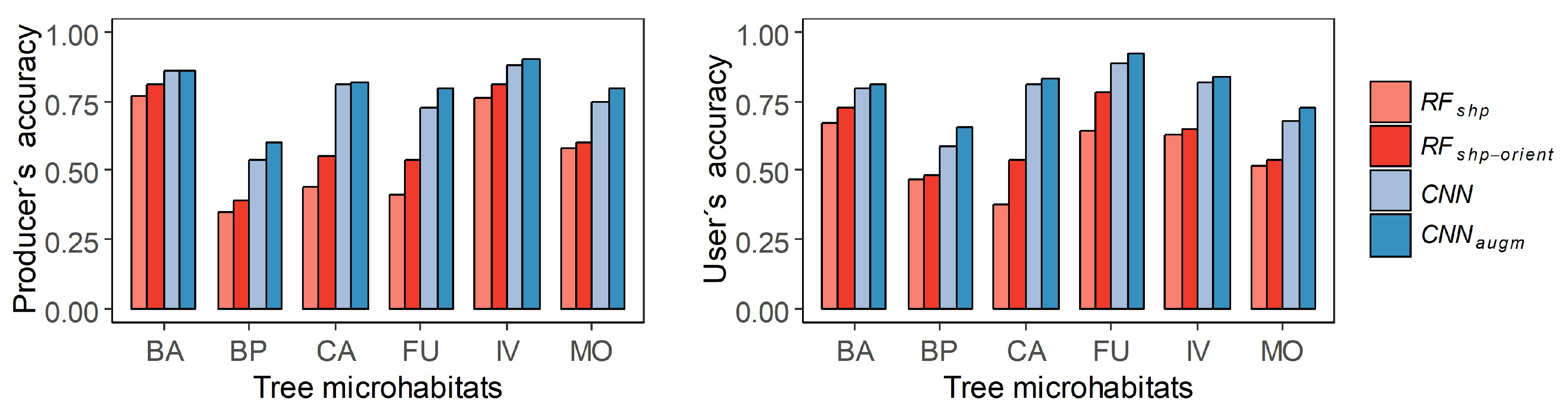
Both accuracy metrics for TreM identification (PA and UA) varied across the classification models (Figure 6). The lowest values were achieved for RFshp and the highest values were realized for CNNaugm. PA showed a similar trend for all classification models, resulting in the highest values for bark and ivy and the lowest for bark pockets. The different groups of TreMs do not benefit in the same way from different classification models. The accuracy metrics for fungi and cavities improved the most (the differences between RFshp and CNNaugm were close to 40%), whereas for bark, the differences were much lower (around 10%). Involving the orientation features slightly improved the identification of all TreM groups with PA and UA increasing most for cavities and fungi (more than 10%). CNNs substantially increased the accuracy metrics of identification of all TreM groups, apart from bark (see Figure 6). Training CNNs on the augmented training set further increased both accuracy metrics of all groups of TreMs by several percents. The best classification model (CNNaugm) resulted in the highest PA for ivy (90%), whereas the highest UA was obtained with fungi (92%). Both accuracy metrics were the lowest for bark pockets (PA = 60%, UA = 66%).
3.2. Patch-Based Predictive Accuracy
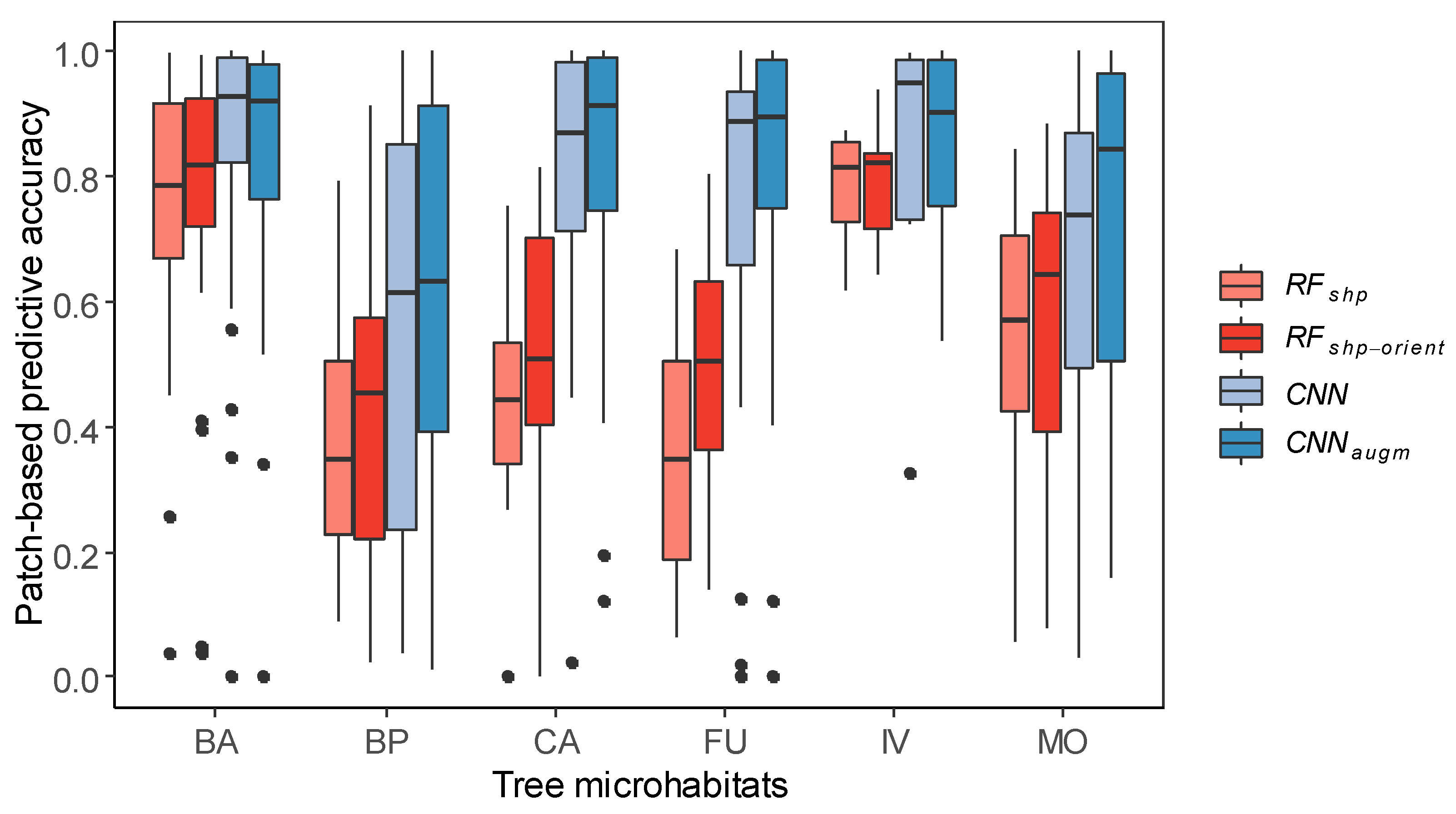
With the LOOCV, predictive accuracies were calculated for each patch (in total, 173 patches). Figure 7 shows that the patch-based predictive accuracies varied greatly across all groups of TreMs and all models. These variations indicate that the patches within each TreM group were not homogeneous. The patch-based predictive accuracies were highest for ivy with the lowest variation. For bark, the predictive accuracies for most of the patches were high for all models, but there were several outliers. CNN models predicted the patches associated with cavities and fungi more accurately, but there were several outliers with low accuracies (<25%). The predictive accuracies varied the most for mosses and bark pockets.
RFshp–orient resulted in a better predictive accuracy of patches for most group of TreMs than RFshp, but also in a higher variability. CNNs produced a better predictive accuracy for most of the groups of TreMs, but did not always reduce the variability within the groups. According to the Kolmogorov–Smirnov significance test, CNN and CNNaugm provided in general a significantly better result (at the 0.05 significance level) in the assessment of most groups of TreMs than RFshp and RFshp–orient (Table 11); for ivy, RFshp produced significantly worse results than all other classification models. The Kolmogorov–Smirnov significance test shows that the patch-based predictive accuracies obtained using RFshp and RFshp–orient, as well as CNN and CNNaugm, were not significantly different.
4. Discussion
In this study, a novel approach was developed for identifying the stem structures associated with six groups of TreMs (bark, bark pockets, cavities, fungi, ivy and mosses) on beech (Fagus sylvatica L.), based on dense TLS point clouds, and applying a semi-automated point-wise semantic labeling. We tested both a classic statistical classifier trained on hand-engineered predictors and a deep learning approach capturing representations directly from the data. RF involving local 3D geometric features has been frequently used in the past decade for the semantic labeling of unstructured 3D point clouds captured in natural environments [34,35]. In contrast, CNNs have experienced more attention in remote sensing only recently, but have already proved to have great potential for both semantic labeling and classification [44,45,46,47,48,49,50].
The classification algorithms, which were used to identify the six TreM groups, produced different results. Whereas the RF classifier produced an OA of up to 70% when both local 3D shape features and two additionally developed orientation features were used, the CNNs significantly outperformed this with an OA of 82% and thus seem potentially better. The proposed rasterized MVOPs of a point’s local 3D neighborhood (top view, front view and side view) seems to be a powerful input data set for a CNN. CNNs also benefited from synthetic transformation of the data (data augmentation), which increased the variability of the training set. The best final agreement was achieved for bark and ivy, whereas it was lowest for bark pockets. The advantages and drawbacks of both classification approaches, as well as the potential and limitations of TLS 3D point clouds for identifying TreMs, are discussed below.
4.1. Local 3D Geometric Features vs. Convolutional Features for TreM Identification
The local 3D geometric features used in this study comprise 3D shape and orientation features. Some of these features have been successfully used in forestry applications for filtering and semantic labeling TLS data. For example, flatness (also planarity) was used to detect single tree-stem profiles [40], and, in combination with verticality, for denoising and modeling tree stems [20]. Eigen decomposition is particularly useful for reconstructing tree architecture [21]. Moreover, geometric features are superior to spectral features for discriminating foliar and woody material in mixed natural forests, but the combination of both provides the best results [41].
Using 2D CNNs for semantic segmentation of 3D point clouds has already been successfully applied in other studies [47,48], where 2D raster data were generated from the initial 3D point clouds and then used to train a CNN. Thus, [47] generated multiple 2D snapshots of the point cloud and produced two types of images: Red-Green-Blue (RGB) view and a depth composite view containing geometric features. In [48], RGB, depth and surface normal images were produced. When generating input data for a classification model, it is important to consider that a 3D object might look different, depending on the perspective and distance to the object. This can be addressed either by choosing different viewing positions (as used in e.g., [47,48]) or by rotating the 3D point cloud around a certain axis, as conducted in this study.
We found that the local 3D geometric features used in this study have a limited potential for identifying the stem structures associated with the six groups of TreMs. These features are powerful for distinguishing between 2D (i.e., bark, mosses) and 3D (i.e., cavities, fungi and ivy) stem structures (see Table 7 and Table 8). However, the differences between convex stem structures (i.e., fungi, ivy, and bark pockets) and concave stem structures (i.e., cavities) are not captured. These stem structures were often confused with each other. Using CNNs incorporating rasterized MVOPs could substantially reduce or even eliminate the misclassifications between TreM groups (see Table 9).
An advantage of the local 3D geometric features is, that in contrast to the rasterized MVOPs, they are robust to global inclinations of a tree stem and thus suitable for both straight and inclined trees. An inclined tree stem can be corrected using a stem axis, but this might be challenging for curved trees. In such cases, generating 2D input data for a CNN using different vertical angles (as used in [46]) or an artificial rotation of the point cloud around a horizontal axis to a certain angle might be beneficial. Integrating both the deep representations learned by CNNs and the local 3D geometric features into a classification model might also be promising. Such an approach has successfully been applied by [50] and also resulted in a higher transferability of the classification model.
In this study, we used two self-developed orientation features. The idea behind these features was to capture local changes in the directions of the stem surface relative to the stem axis. These features were inspired by the verticality feature used by [39], which was calculated as an angular product between the vertical axis and the local normal. Training the RF on the enlarged feature set, which included the two proposed orientation features and other local geometric features used in this study, increased the overall classification accuracy by 4%. To calculate the orientation features, the fitted tree-stem axes were used. Thus, these features might be sensitive to the quality of the stem axes.
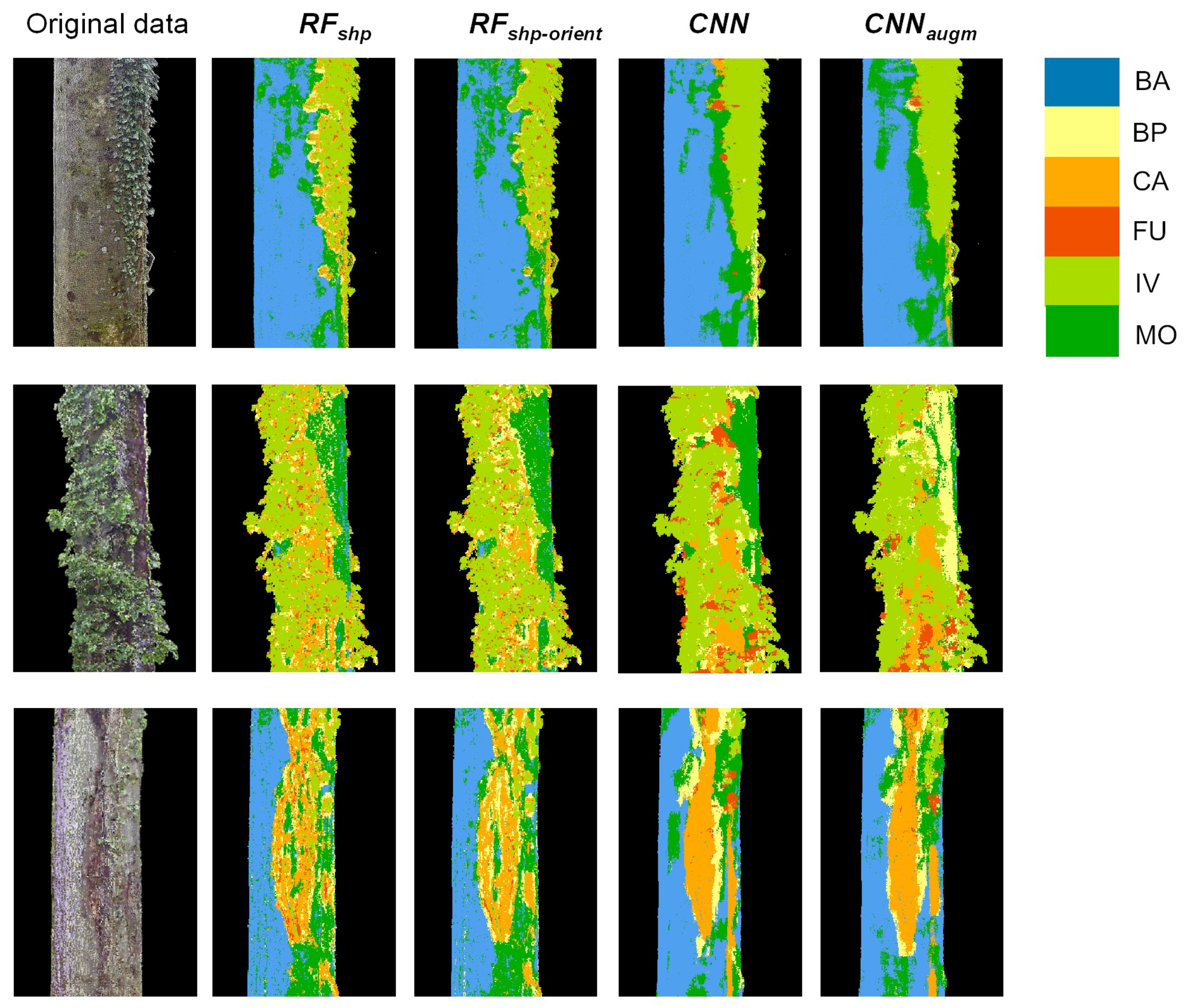
Visual inspection of the point-wise semantic labeling of tree-stem point clouds shows that RF using local 3D geometric features resulted in a more fragmented prediction than CNN classification models (Figure 8). For example, when using RFshp, cavities, fungi and bark pockets were misclassified within the regions of the tree stems covered by ivy (Figure 8, top and middle row). These misclassifications also occur in highly structured stem regions that are associated with large cavities (Figure 8, bottom row). The prediction obtained using the RFshp–orient classification model was only slightly less fragmented.
In general, the predictions of the six groups of TreMs using CNNs were less fragmented and thus better. Although misclassifications were reduced, problems remain in the regions on the tree stems, where several different types of TreMs border each other. In these regions, both RF classification models perform better. However, the set of local geometric features in this study is limited. Other high-level local geometric features, as provided in the literature (e.g., [35]), might be more suitable for TreM identification. The rasterized MVOPs proposed in this study include only the geometric information of the point cloud, i.e., depth in terms of accumulation of the points. Involving 2D images generated from other point cloud information (e.g., normals, as used by [48], or local geometric features) might be beneficial for classification performance.
4.2. Limitations of TLS Data for TreM Identification
Although 3D point clouds have great potential for analyzing tree-stem structures associated with TreMs on beech, they have several limitations:
- (1)
- Occlusion. This is a key factor that limits the use of TLS technology, especially in forest environments. The presence of other trees, branches and foliage material between the scanning device and the target object (habitat tree) may lead to substantial information loss. This can be minimized by using scanning designs with multiple scanner positions [18,19], or by using other technologies, such as a canopy crane [73]. In the present study, occlusions on the stems of the habitat trees were minimized using a single-tree scanning design with multiple scanner positions. Nevertheless, not all TreMs of a habitat tree can be assessed using TLS even with such a scanning design. The TreMs located in the tree crown are very difficult to detect with TLS due to the occlusion with branches and foliage.
- (2)
- Point cloud quality. Tree stems were scanned from multiple positions to detect TreMs. However, the quality of a co-registered point cloud is crucial since this might affect the results of the point cloud interpretation. Visual inspection of the semantic point cloud labeling results revealed that the predictive accuracies for some groups of TreMs may depend on the stem height. For example, identifying bark was more accurate in the lower parts of the tree stems than it was in the upper parts (Figure 9). Detailed inspection of the point clouds showed that the point cloud quality was lower in the upper part of the tree stem, where multiple representations on the tree-stem cross-section were present. Since the scan co-registration using reference targets was reported to be successful, spatial inconsistencies in point clouds in the upper parts of tree stems might occur because of slight movement of tree stem caused by wind. The movement amplitude tends to be zero in lower parts of tree stem, but increases with tree height. Such spatial inconsistencies, especially in the TLS point clouds derived from multiple scanning positions, have been reported to have a significant effect on tree parameter estimation in upper parts of tree stems [74], as well as affecting tree whorl detection and branch modeling [75]. Additional training data collected in the upper stem parts could be useful to overcome this problem when identifying TreMs in TLS point clouds using machine learning approaches, and to improve the classification accuracy.
- (3)
- Spatial resolution. The TLS point clouds used in this study were acquired at a very high spatial resolution (point spacing of 3 mm at 10 m distance). Consequently, the data acquisition was time-consuming. This means it probably cannot yet feasibly be used in the framework of a forest inventory. We hypothesize that reducing the spatial resolution of TLS point clouds may have an effect on TreM identification, especially on TreMs with very fine structures, e.g., mosses, but this has not yet been studied. Another aspect is that the spatial resolution of TLS data decreases with tree-stem height. As a consequence, the structural properties of the objects located in the upper part of the tree stems may be captured with less detail.
- (4)
- Spectral information. Besides spatial information (xyz coordinates), the FARO Focus 3D S120 laser scanner also captures information in the visible and near-infrared (NIR) parts of the light spectrum. As previously mentioned, RGB values are very sensitive to sun illumination and are thus not suitable for analyzing TLS data. Instead, intensity values can be used. [65] reported that intensity values provided by the FARO Focus 3D S120 depend on the distance to the scanned object and proposed an approach to correct it. Authors of [41] used a RIEGL VZ-400 scanner in their study on discriminating foliar and woody material in mixed natural forests. They reported that, beside local geometric features, the features derived from intensity values were highly relevant. We suggest that intensity values could improve the identification of the TreMs containing chlorophyll, i.e., mosses and ivy.
5. Conclusions
Dense point clouds seem to have high potential for the semi-automated identification of stem structures associated with TreMs (bark, bark pockets, cavities, fungi, ivy and mosses), as shown here for beech. Whereas the discriminative power of hand-engineered local geometric features used in this study is limited, deep representatives learned by CNNs from proposed rasterized MVOPs, which denote accumulation of points in the point cloud, are very promising. The best RF classification model trained based on the complete set of the local geometric features resulted in an OA of 70%, whereas with the best CNN incorporating rasterized MVOPs, it was 83%. The local geometric features are very effective in distinguishing between the structures with 2D (bark and mosses) and 3D (cavities, ivy and fungi) properties, whereas they are less useful in distinguishing convex stem structures such as ivy and fungi, and concave structures such as cavities. The rasterized MVOPs are more suitable for the identification of such stem structures. However, further work is needed and more training data should be used to capture TreMs properties better, especially in stem regions where several stem structures may border each other, and where spatial inconsistencies in point clouds caused by wind may occur. Incorporating additional classification approaches, as well as involving an enlarged set of local geometric features might improve TreM identification. Moreover, the approach needs to be tested on other important tree species such as oak, spruce and fir as well. In future, it is necessary to investigate how TreM identification and assessment of the ecological value of a tree or a forest stand might be affected by reduction of point cloud density, the usage of other (lighter) scanning devices with different levels of measurement precision, or information loss due to occlusion.
Author Contributions
Nataliia Rehush is responsible for the study. She developed the methods, collected and analyzed the data and was the main writer of the manuscript. Urs-Beat Brändli developed the idea for the research topic and led the research project, analyzed the Swiss NFI data, contributed to field method development and data collection, and the manuscript revision. Meinrad Abegg and Lars T. Waser contributed to the method development, discussion of the results and the manuscript revision.
Funding
This research was conducted within the scientific project “Assessing stem structures using terrestrial laser scanning” of the Swiss National Forest Inventory. The project was supported by the Swiss Federal Institute of Forest, Snow and Landscape Research (WSL) and the Swiss Federal Office for the Environment (FOEN).
Acknowledgments
The authors would like to thank Björn Wolfgang Dreier, Michael Plüss, Léa Houpert and Amélie Quarteroni for their help during the field survey. We are also grateful to Jonas Stillhard for providing information on habitat trees in Swiss forest reserves, Christian Ginzler for fruitful discussions regarding the scanning design and Silvia Dingwall for professional language editing. Finally, we thank three anonymous reviewers for helping us improve the manuscript.
Conflicts of Interest
The authors declare no conflicts of interest.
References
- FOREST EUROPE, UNECE and FAO. State of Europe’s Forests 2011. In Status and Trends in Sustainable Forest Management in Europe; Ministerial Conference on the Protection of Forests in Europe; FOREST EUROPE: Liaison Unit, Oslo, Norway, 2011. [Google Scholar]
- Fritz, Ö.; Heilmann-Clausen, J. Rot holes create key microhabitats for epiphytic lichens and bryophytes on beech (Fagus sylvatica). Biol. Conserv. 2010, 143, 1008–1016. [Google Scholar] [CrossRef]
- Regnery, B.; Couvet, D.; Kubarek, L.; Julien, J.-F.; Kerbiriou, C. Tree microhabitats as indicators of bird and bat communities in Mediterranean forests. Ecol. Indic. 2013, 34, 221–230. [Google Scholar] [CrossRef]
- Bütler, R.; Lachat, T.; Larrieu, L.; Paillet, Y. Habitat trees: Key elements for forest biodiversity. In Integrative Approaches as an Opportunity for the Conservation of Forest Biodiversity; European Forest Institute: Joensuu, Finland, 2013; pp. 84–91. [Google Scholar]
- Franks, D.C.; Reeves, J.W. A formula for assessing the ecological value of trees. J. Arboric. 1988, 14, 255–259. [Google Scholar]
- Winter, S.; Möller, G.C. Microhabitats in lowland beech forests as monitoring tool for nature conservation. For. Ecol. Manag. 2008, 255, 1251–1261. [Google Scholar] [CrossRef]
- Quarteroni, A.; Brändli, U.-B. Les dendromicrohabitats dans l’Inventaire Forestier National suisse. Infoblatt Arbeitsgruppe Waldplanung-Manag. 2017, 14, 10–14. [Google Scholar]
- Larrieu, L.; Cabanettes, A. Species, live status, and diameter are important tree features for diversity and abundance of tree microhabitats in subnatural montane beech–fir forests. Can. J. For. Res. 2012, 42, 1433–1445. [Google Scholar] [CrossRef]
- Vuidot, A.; Paillet, Y.; Archaux, F.; Gosselin, F. Influence of tree characteristics and forest management on tree microhabitats. Biol. Conserv. 2011, 144, 441–450. [Google Scholar] [CrossRef]
- Brändli, U.-B.; Abegg, M.; Bütler, R. Lebensraum-Hotspots für saproxylische Arten mittels LFI-Daten erkennen. Schweiz. Z. Forstwes. 2011, 162, 312–325. [Google Scholar] [CrossRef]
- Paillet, Y.; Coutadeur, P.; Vuidot, A.; Archaux, F.; Gosselin, F. Strong observer effect on tree microhabitats inventories: A case study in a French lowland forest. Ecol. Indic. 2015, 49, 14–23. [Google Scholar] [CrossRef]
- Larrieu, L.; Paillet, Y.; Winter, S.; Bütler, R.; Kraus, D.; Krumm, D.; Lachat, T.; Michel, A.K.; Regnery, B.; Vandekerkhove, K. Tree related microhabitats in temperate and Mediterranean European forests: A hierarchical typology for inventory standardization. Ecol. Indic. 2018, 84, 194–207. [Google Scholar] [CrossRef]
- McRoberts, R.E.; Chirici, G.; Winter, S.; Barbati, A.; Corona, P.; Marchetti, M.; Hauk, E.; Brändli, U.-B.; Beranova, J.; Rondeux, J.; et al. Prospects for Harmonized Biodiversity Assessments Using National Forest Inventory Data. In National Forest Inventories: Contributions to Forest Biodiversity Assessments; Managing Forest Ecosystems; Springer: Dordrecht, The Netherlands, 2011; pp. 41–97. ISBN 978-94-007-0481-7. [Google Scholar]
- Barrett, F.; McRoberts, R.E.; Tomppo, E.; Cienciala, E.; Waser, L.T. A questionnaire-based review of the operational use of remotely sensed data by national forest inventories. Remote Sens. Environ. 2016, 174, 279–289. [Google Scholar] [CrossRef]
- Liang, X.; Hyyppä, J.; Kaartinen, H.; Lehtomäki, M.; Pyörälä, J.; Pfeifer, N.; Holopainen, M.; Brolly, G.; Francesco, P.; Hackenberg, J.; et al. International benchmarking of terrestrial laser scanning approaches for forest inventories. ISPRS J. Photogramm. Remote Sens. 2018, 144, 137–179. [Google Scholar] [CrossRef]
- Liang, X.; Kankare, V.; Hyyppä, J.; Wang, Y.; Kukko, A.; Haggrén, H.; Yu, X.; Kaartinen, H.; Jaakkola, A.; Guan, F.; et al. Terrestrial laser scanning in forest inventories. ISPRS J. Photogramm. Remote Sens. 2016, 115, 63–77. [Google Scholar] [CrossRef] [Green Version]
- White, J.C.; Coops, N.C.; Wulder, M.A.; Vastaranta, M.; Hilker, T.; Tompalski, P. Remote Sensing Technologies for Enhancing Forest Inventories: A Review. Can. J. Remote Sens. 2016, 42, 619–641. [Google Scholar] [CrossRef]
- Abegg, M.; Kükenbrink, D.; Zell, J.; Schaepman, M.E.; Morsdorf, F. Terrestrial laser scanning for forest inventories—Tree diameter distribution and scanner location impact on occlusion. Forests 2017, 8, 184. [Google Scholar] [CrossRef]
- Heinzel, J.; Huber, M.O. Detecting tree stems from volumetric TLS data in forest environments with rich understory. Remote Sens. 2017, 9, 17. [Google Scholar] [CrossRef]
- de Conto, T.; Olofsson, K.; Görgens, E.B.; Rodriguez, L.C.E.; Almeida, G. Performance of stem denoising and stem modelling algorithms on single tree point clouds from terrestrial laser scanning. Comput. Electron. Agric. 2017, 143, 165–176. [Google Scholar] [CrossRef]
- Hackenberg, J.; Spiecker, H.; Calders, K.; Disney, M.; Raumonen, P. SimpleTree—An Efficient Open Source Tool to Build Tree Models from TLS Clouds. Forests 2015, 6, 4245–4294. [Google Scholar] [CrossRef]
- Raumonen, P.; Kaasalainen, M.; Åkerblom, M.; Kaasalainen, S.; Kaartinen, H.; Vastaranta, M.; Holopainen, M.; Disney, M.; Lewis, P. Fast Automatic Precision Tree Models from Terrestrial Laser Scanner Data. Remote Sens. 2013, 5, 491–520. [Google Scholar] [CrossRef] [Green Version]
- Åkerblom, M.; Raumonen, P.; Mäkipää, R.; Kaasalainen, M. Automatic tree species recognition with quantitative structure models. Remote Sens. Environ. 2017, 191, 1–12. [Google Scholar] [CrossRef]
- Othmani, A.; Jiang, C.; Lomenie, N.; Favreau, J.-M.; Piboule, A.; Voon, L.F.C.L.Y. A novel Computer-Aided Tree Species Identification method based on Burst Wind Segmentation of 3D bark textures. Mach. Vis. Appl. 2016, 27, 751–766. [Google Scholar] [CrossRef]
- Heinzel, J.; Huber, M.O. Tree stem diameter estimation from volumentric TLS image data. Remote Sens. 2017, 9, 614. [Google Scholar] [CrossRef]
- Béland, M.; Baldocchi, D.D.; Widlowski, J.-L.; Fournier, R.A.; Verstraete, M.M. On seeing the wood from the leaves and the role of voxel size in determining leaf area distribution of forests with terrestrial LiDAR. Agric. For. Meteorol. 2014, 184, 82–97. [Google Scholar] [CrossRef]
- Dassot, M.; Colin, A.; Santenoise, P.; Fournier, M.; Constant, T. Terrestrial laser scanning for measuring the solid wood volume, including branches, of adult standing trees in the forest environment. Comput. Electron. Agric. 2012, 89, 86–93. [Google Scholar] [CrossRef]
- Stängle, S.M.; Brüchert, F.; Kretschmer, U.; Spiecker, H.; Sauter, U.H. Clear wood content in standing trees predicted from branch scar measurements with terrestrial LiDAR and verified with X-ray computed tomography. Can. J. For. Res. 2014, 44, 145–153. [Google Scholar] [CrossRef]
- Nguyen, V.-T.; Kerautret, B.; Debled-Rennesson, I.; Colin, F.; Piboule, A.; Constant, T. Segmentation of defects on log surface from terrestrial lidar data. In Proceedings of the 23rd International Conference on Pattern Recognition (ICPR), Cancun, Mexico, 4–8 December 2016; pp. 3168–3173. [Google Scholar]
- Kankare, V.; Vauhkonen, J.; Tanhuanpää, T.; Holopainen, M.; Vastaranta, M.; Joensuu, M.; Krooks, A.; Hyyppä, J.; Hyyppä, H.; Alho, P.; et al. Accuracy in estimation of timber assortments and stem distribution—A comparison of airborne and terrestrial laser scanning techniques. ISPRS J. Photogramm. Remote Sens. 2014, 97, 89–97. [Google Scholar] [CrossRef]
- Aschoff, T.; Spieker, H.; Holderied, M.W. Terrestrische Laserscanner und akustische Ortungssysteme: Jagdlebensräume von Fledermäusen in Wäldern. AFZ Wald 2007, 62, 172–175. [Google Scholar]
- Michel, P.; Jenkins, J.; Mason, N.; Dickinson, K.J.M.; Jamieson, I.G. Assessing the ecological application of lasergrammetric techniques to measure fine-scale vegetation structure. Ecol. Inform. 2008, 3, 309–320. [Google Scholar] [CrossRef]
- Schnabel, R.; Wahl, R.; Klein, R. Efficient RANSAC for Point-Cloud Shape Detection. Comput. Graph. Forum 2007, 26, 214–226. [Google Scholar] [CrossRef] [Green Version]
- Brodu, N.; Lague, D. 3D terrestrial lidar data classification of complex natural scenes using a multi-scale dimensionality criterion: Applications in geomorphology. ISPRS J. Photogramm. Remote Sens. 2012, 68, 121–134. [Google Scholar] [CrossRef] [Green Version]
- Weinmann, M.; Jutzi, B.; Hinz, S.; Mallet, C. Semantic point cloud interpretation based on optimal neighborhoods, relevant features and efficient classifiers. ISPRS J. Photogramm. Remote Sens. 2015, 105, 286–304. [Google Scholar] [CrossRef]
- Ghosh, A.; Fassnacht, F.E.; Joshi, P.K.; Koch, B. A framework for mapping tree species combining hyperspectral and LiDAR data: Role of selected classifiers and sensor across three spatial scales. Int. J. Appl. Earth Obs. Geoinf. 2014, 26, 49–63. [Google Scholar] [CrossRef]
- Belgiu, M.; Drăguţ, L. Random forest in remote sensing: A review of applications and future directions. ISPRS J. Photogramm. Remote Sens. 2016, 114, 24–31. [Google Scholar] [CrossRef]
- Guo, Y.; Bennamoun, M.; Sohel, F.; Lu, M.; Wan, J.; Kwok, N.M. A Comprehensive Performance Evaluation of 3D Local Feature Descriptors. Int. J. Comput. Vis. 2016, 116, 66–89. [Google Scholar] [CrossRef]
- Hackel, T.; Wegner, J.D.; Schindler, K. Joint classification and contour extraction of large 3D point clouds. ISPRS J. Photogramm. Remote Sens. 2017, 130, 231–245. [Google Scholar] [CrossRef]
- Olofsson, K.; Holmgren, J. Single Tree Stem Profile Detection Using Terrestrial Laser Scanner Data, Flatness Saliency Features and Curvature Properties. Forests 2016, 7, 207. [Google Scholar] [CrossRef]
- Zhu, X.; Skidmore, A.K.; Darvishzadeh, R.; Niemann, K.O.; Liu, J.; Shi, Y.; Wang, T. Foliar and woody materials discriminated using terrestrial LiDAR in a mixed natural forest. Int. J. Appl. Earth Obs. Geoinformation 2018, 64, 43–50. [Google Scholar] [CrossRef]
- Ball, J.E.; Anderson, D.T.; Chan, C.S. Comprehensive survey of deep learning in remote sensing: Theories, tools, and challenges for the community. J. Appl. Remote Sens. 2017, 11, 042609. [Google Scholar] [CrossRef]
- Bengio, Y.; Courville, A.; Vincent, P. Representation Learning: A Review and New Perspectives. IEEE Trans. Pattern Anal. Mach. Intell. 2013, 35, 1798–1828. [Google Scholar] [CrossRef] [PubMed] [Green Version]
- Huang, J.; You, S. Point Cloud Labeling using 3D Convolutional Neural Network. In Proceedings of the 23rd International Conference on Pattern Recognition (ICPR), Cancún, Mexico, 4–8 December 2016; pp. 2670–2675. [Google Scholar]
- Maturana, D.; Scherer, S. VoxNet: A 3D Convolutional Neural Network for Real-Time Object Recognition. In Proceedings of the IEEE/RSJ International Conference on Intelligent Robots and Systems (IROS), Hamburg, Germany, 28 September–2 October 2015; pp. 922–928. [Google Scholar]
- Ayrey, E.; Hayes, D.J. The Use of Three-Dimensional Convolutional Neural Networks to Interpret LiDAR for Forest Inventory. Remote Sens. 2018, 10, 649. [Google Scholar] [CrossRef]
- Boulch, A.; Guerry, J.; Le Saux, B.; Audebert, N. SnapNet: 3D point cloud semantic labeling with 2D deep segmentation networks. Comput. Graph. 2018, 71, 189–198. [Google Scholar] [CrossRef]
- Lawin, F.J.; Danelljan, M.; Tosteberg, P.; Bhat, G.; Khan, F.S.; Felsberg, M. Deep Projective 3D Semantic Segmentation. In Proceedings of the 17th International Conference on Computer Analysis of Images and Patterns, Ystad, Sweden, 22–24 August 2017; pp. 95–107. [Google Scholar]
- Yu, H.; Yang, Z.; Tan, L.; Wang, Y.; Sun, W.; Sun, M.; Tang, Y. Methods and datasets on semantic segmentation: A review. Neurocomputing 2018, 304, 82–103. [Google Scholar] [CrossRef]
- Vetrivel, A.; Gerke, M.; Kerle, N.; Nex, F.; Vosselman, G. Disaster damage detection through synergistic use of deep learning and 3D point cloud features derived from very high resolution oblique aerial images, and multiple-kernel-learning. ISPRS J. Photogramm. Remote Sens. 2018, 140, 45–59. [Google Scholar] [CrossRef]
- Inventaire Forestier National Suisse. Résultats du Troisième Inventaire 2004–2006; Brändli, U.-B. (Ed.) Birmensdorf, Institut Fédéral de Recherches sur la Forêt: Switzerland; la Neige et le Paysage WSL; Office Fédéral de L’environnement, OFEV: Berne, Switzerland, 2010. [Google Scholar]
- Inventory of the Largest Primeval Beech Forest in Europe. A Swiss-Ukrainian Scientific Adventure; Commarmot, B.; Brändli, U.-B.; Hamor, F.; Lavnyy, V. (Eds.) Swiss Federal Research Institute WSL; Ukrainian National Forestry University: L’viv, Ukraine; Carpathian Biosphere Reserve: Rakhiv, Ukraine, 2013. [Google Scholar]
- Schweizerisches Landesforstinventar. Feldaufnahme-Anleitung 2018; Düggelin, C. (Ed.) Eidgenössische Forschungsanstalt für Wald, Schnee und Landschaft WSL: Birmensdorf, Schweiz, in preparation.
- CloudCompare—3D Point Cloud and Mesh Processing Software [GPL software]. Version 2.9. Available online: http://www.cloudcompare.org/ (accessed on 27 September 2018).
- Rusu, R.B.; Marton, Z.C.; Blodow, N.; Dolha, M.; Beetz, M. Towards 3D Point cloud based object maps for household environments. Robot. Auton. Syst. 2008, 56, 927–941. [Google Scholar] [CrossRef]
- Kretschmer, U.; Kirchner, N.; Morhart, C.; Spiecker, H. A new approach to assessing tree stem quality characteristics using terrestrial laser scans. Silva Fenn. 2013, 47. [Google Scholar] [CrossRef]
- Dittrich, A.; Weinmann, M.; Hinz, S. Analytical and numerical investigations on the accuracy and robustness of geometric features extracted from 3D point cloud data. ISPRS J. Photogramm. Remote Sens. 2017, 126, 195–208. [Google Scholar] [CrossRef]
- Bishop, C.M.; Roach, C.M. Fast curve fitting using neural networks. Rev. Sci. Instrum. 1992, 63, 4450–4456. [Google Scholar] [CrossRef]
- Breiman, L. Random Forests. Mach. Learn. 2001, 45, 5–32. [Google Scholar] [CrossRef] [Green Version]
- Breiman, L. Bagging Predictors. Mach. Learn. 1996, 24, 123–140. [Google Scholar] [CrossRef]
- Hastie, T.; Tibshirani, R.; Friedman, J. The Elements of Statistical Learning: Data Mining, Inference, and Prediction, 2nd ed.; Springer Series in Statistics; Springer: New York, NY, USA, 2009; ISBN 978-0-387-84857-0. [Google Scholar]
- Immitzer, M.; Atzberger, C.; Koukal, T. Tree Species Classification with Random Forest Using Very High Spatial Resolution 8-Band WorldView-2 Satellite Data. Remote Sens. 2012, 4, 2661–2693. [Google Scholar] [CrossRef] [Green Version]
- Lawrence, R.L.; Wood, S.D.; Sheley, R.L. Mapping invasive plants using hyperspectral imagery and Breiman Cutler classifications (randomForest). Remote Sens. Environ. 2006, 100, 356–362. [Google Scholar] [CrossRef]
- Kuhn, M. Building predictive models in R using the caret package. J. Stat. Softw. 2008, 28. [Google Scholar] [CrossRef]
- Heinzel, J.; Huber, M.O. TLS field data based intensity correction for forest environments. Int. Arch. Photogramm. Remote Sens. Spat. Inf. Sci. 2016, XLI-B8, 643–649. [Google Scholar] [CrossRef]
- LeCun, Y.; Boser, B.; Denker, J.S.; Henderson, D.; Howard, R.E.; Hubbard, W.; Jackel, L.D. Backpropagation Applied to Handwritten Zip Code Recognition. Neural Comput. 1989, 1, 541–551. [Google Scholar] [CrossRef]
- Krizhevsky, A.; Sutskever, I.; Hinton, G. ImageNet classification with deep convolutional neural networks. In Proceedings of the Advances in Neural Information Processing Systems (NIPS), Lake Tahoe, Nevada, 3–6 December 2012; pp. 1097–1105. [Google Scholar]
- Srivastava, N.; Hinton, G.; Krizhevsky, A.; Sutskever, I.; Salakhutdinov, R. Dropout: A Simple Way to Prevent Neural Networks from Overfitting. J. Mach. Learn. Res. 2014, 15, 1929–1958. [Google Scholar]
- Goodfellow, I.; Bengio, Y.; Courville, A. Deep Learning; MIT Press: Cambridge, MA, USA, 2016. [Google Scholar]
- Carlbom, I.; Paciorek, J. Planar Geometric Projections and Viewing Transformations. ACM Comput. Surv. 1978, 10, 465–502. [Google Scholar] [CrossRef] [Green Version]
- Stone, M. Cross-Validatory Choice and Assessment of Statistical Predictions. J. R. Stat. Soc. Ser. B Methodol. 1974, 36, 111–147. [Google Scholar]
- Foody, G.M. Status of land cover classification accuracy assessment. Remote Sens. Environ. 2002, 80, 185–201. [Google Scholar] [CrossRef]
- Morsdorf, F.; Kükenbrink, D.; Schneider, F.D.; Abegg, M.; Schaepman, M.E. Close-range laser scanning in forests: Towards physically based semantics across scales. Interface Focus 2018, 8, 10. [Google Scholar] [CrossRef] [PubMed]
- Vaaja, M.T.; Virtanen, J.-P.; Kurkela, M.; Lehtola, V.; Hyyppä, J.; Hyyppä, H. Hannu The Effect of Wind on Tree Stem Parameter Estimation Using Terrestial Laser Scanning. In Proceedings of the ISPRS Annals of the Photogrammetry, Remote Sensing and Spatial Information Sciences, Prague, Czech Republic, 12–19 July 2016; pp. 117–122. [Google Scholar]
- Pyörälä, J.; Liang, X.; Vastaranta, M.; Saarinen, N.; Kankare, V.; Wang, Y.; Holopainen, M.; Hyyppä, J. Quantitative Assessment of Scots Pine (Pinus SylvestrisL.) Whorl Structure in a Forest Environment Using Terrestrial Laser Scanning. IEEE J. Sel. Top. Appl. Earth Obs. Remote Sens. 2018, 11, 3598–3607. [Google Scholar] [CrossRef]
Figure 1.
Workflow for stem axis fitting: (a) original tree-stem point cloud; (b) calculation of planarity feature based on a fixed-radius point’s local neighborhood, which was considered to be within a sphere with a radius of 5 cm; (c) filtering out leaves and small tree branches; (d) “unrolling” the tree stem—xyz coordinates were transformed into Lzd using a cylinder fitted into the point cloud, where L is the length of circumference (m), z—z coordinate of the initial point cloud (m), d—distance to modeled cylinder surface (m); (e,f) filtering out the points located closest to the tree stem surface; (g) fitting the stem axis: the centers of the circles used for stem-axis fitting are in blue and the resulting stem axis in red.

Figure 2.
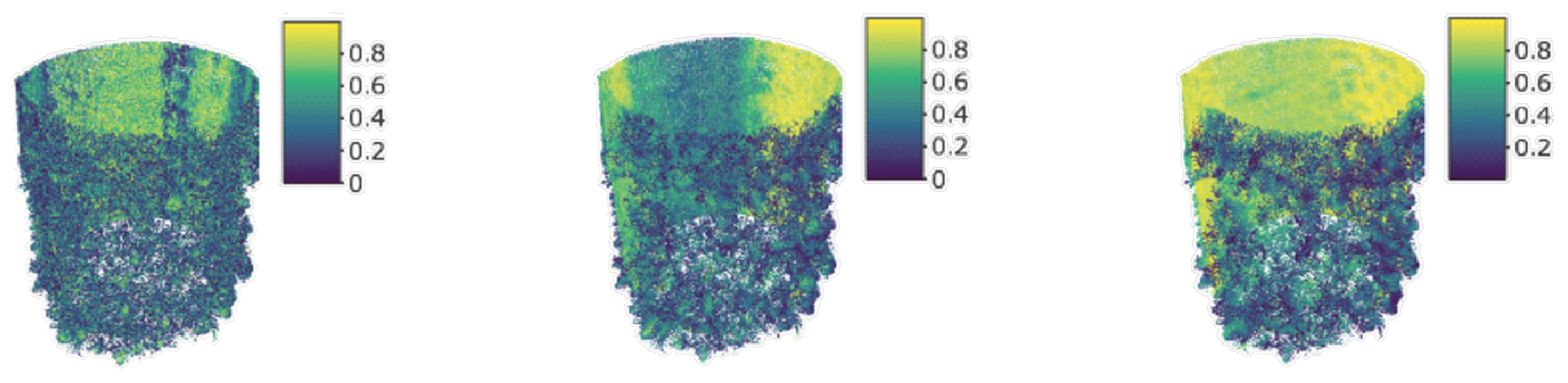
Visualization of a local geometric feature (planarity), calculated for section of the tree stem partly covered with ivy, with scales of 1 cm, 2.5 cm and 5 cm (from left to right) for the point’s local neighborhoods. The local geometric features calculated on a small scale indicate small structures on the tree-stem surface, while those calculated on a bigger scale indicate more rough structures.
Figure 2.
Visualization of a local geometric feature (planarity), calculated for section of the tree stem partly covered with ivy, with scales of 1 cm, 2.5 cm and 5 cm (from left to right) for the point’s local neighborhoods. The local geometric features calculated on a small scale indicate small structures on the tree-stem surface, while those calculated on a bigger scale indicate more rough structures.

Figure 3.
Architecture of the Convolutional Neural Network used in this study: Input indicates the input data (a stack of rasterized multiview orthographic projections), Conv: a convolutional layer, Max pool: a pooling layer calculating a maximum value, and Full: a fully connected layer.
Figure 3.
Architecture of the Convolutional Neural Network used in this study: Input indicates the input data (a stack of rasterized multiview orthographic projections), Conv: a convolutional layer, Max pool: a pooling layer calculating a maximum value, and Full: a fully connected layer.

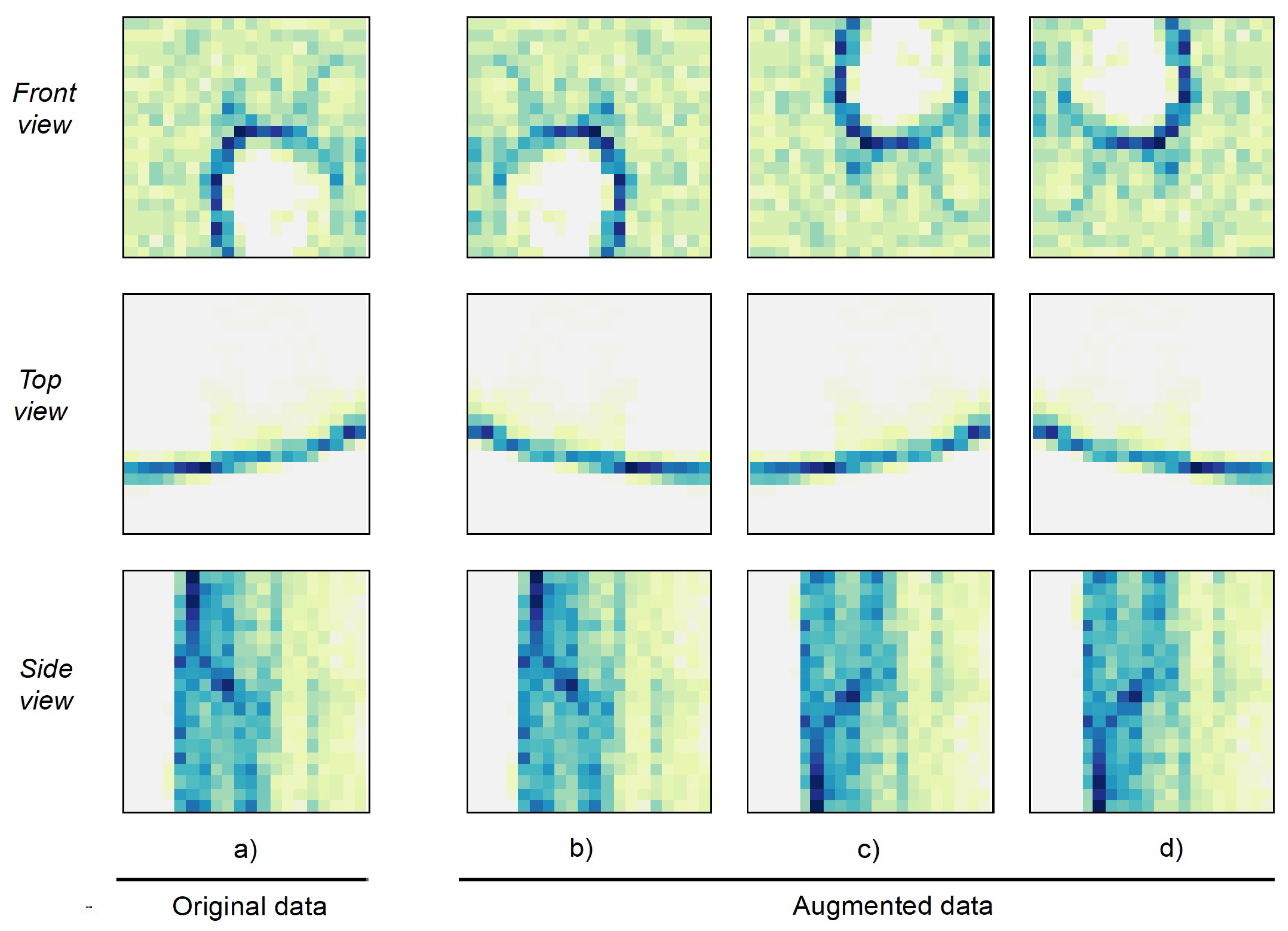
Figure 4.
Generating rasterized multiview orthographic projections (top view, front view and side view) for: (a) bark (BA), (b) bark pockets (BP), (c) cavities (CA), (d) fungi (FU), (e) ivy (IV), and (f) mosses (MO). The color gradient indicates the point accumulation: low in yellow, and high in dark blue.

Figure 5.
Data augmentation: rasterized multiview orthographic projections of (a) the original point cloud and after flipping along the (b) yz, (c) xy, (d) xy and yz planes.
Figure 5.
Data augmentation: rasterized multiview orthographic projections of (a) the original point cloud and after flipping along the (b) yz, (c) xy, (d) xy and yz planes.

Figure 6.
Dynamics of producer’s accuracy (PA) and user’s accuracy (UA) for six groups of TreMs: bark (BA), bark pocket (BP), cavities (CA), fungi (FU), ivy (IV) and mosses (MO).
Figure 6.
Dynamics of producer’s accuracy (PA) and user’s accuracy (UA) for six groups of TreMs: bark (BA), bark pocket (BP), cavities (CA), fungi (FU), ivy (IV) and mosses (MO).

Figure 7.
Distributions of patch-based predictive accuracies of six groups of TreMs obtained using RFshp, RFshp–orient, CNN and CNNaugm. The values were calculated for each of the 173 patches associated with the six groups of TreMs: bark (BA), bark pocket (BP), cavities (CA), fungi (FU), ivy (IV) and mosses (MO).

Figure 8.
Examples of semantic labeling results for parts of a tree stem with ivy and mosses (top row), with ivy, mosses and cavities (middle row), and with cavities (bottom row).
Figure 8.
Examples of semantic labeling results for parts of a tree stem with ivy and mosses (top row), with ivy, mosses and cavities (middle row), and with cavities (bottom row).

Figure 9.
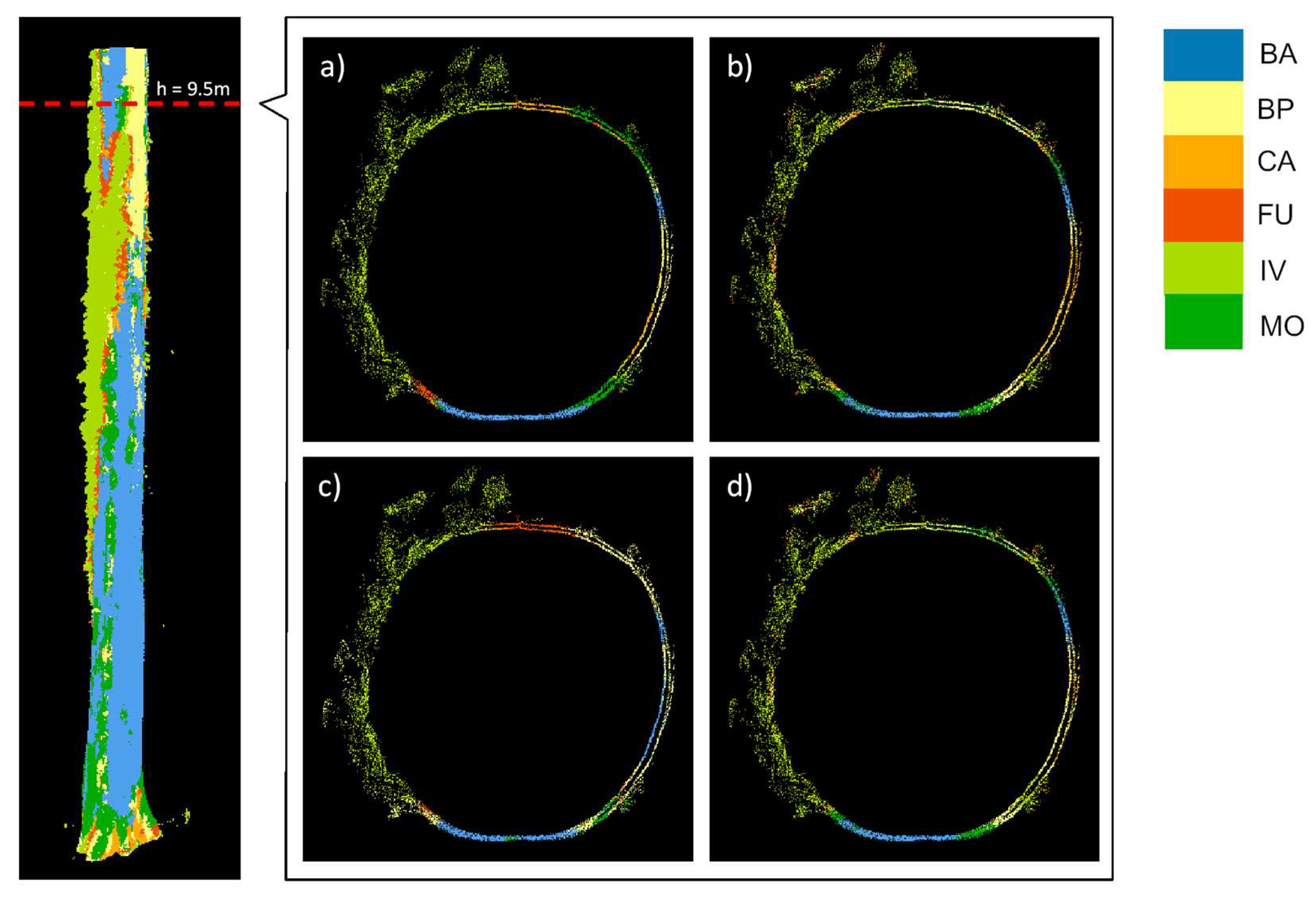
Misclassifications arising from scan co-registration errors. The tree-stem point cloud was labeled using a deep Convolutional Neural Network (left). In the upper part of the tree stem, bark (BA) was misclassified as bark pockets (BP) but it was correctly classified in the lower part of the tree stem. Detailed inspection shows such misclassifications occurred in the regions of the point cloud where scan co-registration failed (right), independent of the classification model used. The cross-sections were collected at h = 9.5 m in the tree-stem point clouds and labeled using the (a) RFshp, (b) RFshp–orient, (c) CNN and (d) CNNaugm classification models.
Figure 9.
Misclassifications arising from scan co-registration errors. The tree-stem point cloud was labeled using a deep Convolutional Neural Network (left). In the upper part of the tree stem, bark (BA) was misclassified as bark pockets (BP) but it was correctly classified in the lower part of the tree stem. Detailed inspection shows such misclassifications occurred in the regions of the point cloud where scan co-registration failed (right), independent of the classification model used. The cross-sections were collected at h = 9.5 m in the tree-stem point clouds and labeled using the (a) RFshp, (b) RFshp–orient, (c) CNN and (d) CNNaugm classification models.


Table 1.
Technical specifications of the FARO Focus 3D S120 laser scanner.
| Ranging unit | Range | 0.6–120 m |
| Ranging error | ±2 mm | |
| Deflection unit | Field of view (vertical/horizontal) | 305°/360° |
| Step size (vertical/horizontal) | 0.009°/0.009° | |
| Laser | Wavelength | 905 nm |
| Beam diameter at exit | 3.0 mm | |
| Beam divergence | 0.011° |
Table 2.
Scanning design used in the study.
| Parameter | Setting |
|---|---|
| Number of scans per tree | 6 |
| Angular resolution (vertical/horizontal) | 0.018°/0.018° |
| Distance from scanner to tree | 5–7 m |
| RGB images | Yes |
| Intensity | Yes |
Table 3.
Definitions of the tree-related microhabitats (TreMs) addressed in the study.
| TreM Type | Definition | Threshold for Inclusion |
|---|---|---|
| Bark loss and exposed wood | Exposed wood and missing bark | Coverage > 1% |
| Bark pocket | Space between peeled-off bark and sapwood forming a pocket (open at the top) or shelter (open at the bottom) | Depth > 1 cm |
| Crack | Crack through the bark or the wood | Width > 1 cm |
| Fungi | Tough fruiting bodies of perennial polypores | Diameter > 2 cm |
| Ivy | Tree stem covered with ivy | Coverage > 1% |
| Lichen | Tree stem covered with foliose and fruticose lichens | Coverage > 1% |
| Moss | Tree stem covered with moss | Coverage > 1% |
| Stem hole | Tree stem rot-hole; cavities resulting from an injury or branch loss | Length > 2 cm, |
| width > 2 cm | ||
| Woodpecker cavity | Woodpecker foraging excavation | Length > 2 cm, |
| width > 2 cm | ||
| Woodpecker hole | Woodpecker breeding cavities | Diameter > 4 cm |
Table 4.
Setups of the classification models trained for automatic identification of TreMs.
| Classification Model | Classifier | Input Data | Input Data Pre-Processing |
|---|---|---|---|
| RFshp | Random Forest | 3D shape features () | None |
| RFshp–orient | Random Forest | 3D shape features + orientation features () | None |
| CNN | Convolutional Neural Network | rasterized multiview orthographic projections | None |
| CNNaugm | Convolutional Neural Network | rasterized multiview orthographic projections | Augmentation |
Table 5.
Sample set used in this study with TreM types included into TreM groups, number of trees used to collect point patches, and number of patches collected for each TreM group.
Table 5.
Sample set used in this study with TreM types included into TreM groups, number of trees used to collect point patches, and number of patches collected for each TreM group.
| TreM Groups | TreM Types Included in the Group | Number of Trees Where Patches Were Collected | Number of Patches | Number of Points |
|---|---|---|---|---|
| Bark | Bark and exposed wood | 10 | 43 | 761,820 |
| Bark pockets | Bark pockets | 8 | 35 | 220,420 |
| Cavities | Cracks, stem holes, woodpecker cavities and holes | 7 | 29 | 150,560 |
| Fungi | Fungi | 6 | 19 | 31,770 |
| Ivy | Ivy (foliage only) | 4 | 15 | 506,210 |
| Mosses | Mosses and lichens | 10 | 32 | 309,235 |
Table 6.
Set of local 3D geometric features as used in this study. The features were derived from eigenvalues and eigenvectors of the covariance tensor of a point’s local 3D neighborhood, which was defined on different scales varying from rmin = 1 cm to rmax = 5 cm with ∆r = 0.5 cm.
Table 6.
Set of local 3D geometric features as used in this study. The features were derived from eigenvalues and eigenvectors of the covariance tensor of a point’s local 3D neighborhood, which was defined on different scales varying from rmin = 1 cm to rmax = 5 cm with ∆r = 0.5 cm.
| Feature Family | Feature Based on a Local 3D Structure Tensor | Feature Definition |
|---|---|---|
| 3D shape features | First eigenvalue | |
| Second eigenvalue | ||
| Linearity | ||
| Planarity | ||
| Sphericity | ||
| Omnivariance | ||
| Anisotropy | ||
| Eigenentropy | ||
| Surface variation | ||
| Orientation features | 3D orientation | |
| 2D orientation |
Table 7.
Error matrix after the patch-based leave-one-out cross-validation (LOOCV) of RF classification models based on 3D shape features (RFshp) for the identification of the six groups of TreMs: bark (BA), bark pockets (BP), cavities (CA), fungi (FU), ivy (IV) and mosses (MO). The performance of the models was assessed using LOOCV. In total, 173 models were trained, each predicted on the points belonging to the “leaved-out” patch.
| Reference | Prediction | Producer’s Accuracy | |||||
|---|---|---|---|---|---|---|---|
| BA | BP | CA | FU | IV | MO | ||
| BA | 0.77 | 0.03 | 0.01 | 0.00 | 0.00 | 0.18 | 0.77 |
| BP | 0.11 | 0.35 | 0.18 | 0.04 | 0.11 | 0.21 | 0.35 |
| CA | 0.03 | 0.15 | 0.44 | 0.13 | 0.13 | 0.13 | 0.44 |
| FU | 0.00 | 0.06 | 0.32 | 0.41 | 0.21 | 0.00 | 0.41 |
| IV | 0.00 | 0.06 | 0.12 | 0.05 | 0.76 | 0.01 | 0.76 |
| MO | 0.24 | 0.09 | 0.08 | 0.00 | 0.01 | 0.58 | 0.58 |
| User’s accuracy | 0.67 | 0.47 | 0.38 | 0.64 | 0.63 | 0.52 | - |
| Overall accuracy: 0.661, Kappa: 0.553 | |||||||
Table 8.
Error matrix after the patch-based LOOCV of RF classification models based on 3D shape and orientation features (RFshp–orient) for the identification of the six groups of TreMs: bark (BA), bark pockets (BP), cavities (CA), fungi (FU), ivy (IV) and mosses (MO). The performance of the models was assessed using LOOCV. In total, 173 models were trained, each predicted on the points belonging to the “leaved-out” patch.
| Reference | Prediction | Producer’s Accuracy | |||||
|---|---|---|---|---|---|---|---|
| BA | BP | CA | FU | IV | MO | ||
| BA | 0.81 | 0.03 | 0.00 | 0.00 | 0.00 | 0.16 | 0.81 |
| BP | 0.08 | 0.39 | 0.17 | 0.03 | 0.11 | 0.23 | 0.39 |
| CA | 0.01 | 0.15 | 0.55 | 0.07 | 0.12 | 0.11 | 0.55 |
| FU | 0.00 | 0.07 | 0.18 | 0.54 | 0.20 | 0.00 | 0.54 |
| IV | 0.00 | 0.05 | 0.07 | 0.06 | 0.81 | 0.01 | 0.81 |
| MO | 0.22 | 0.13 | 0.05 | 0.00 | 0.01 | 0.60 | 0.60 |
| User’s accuracy | 0.73 | 0.48 | 0.54 | 0.78 | 0.65 | 0.54 | - |
| Overall accuracy: 0.704, Kappa: 0.608 | |||||||
Table 9.
Error matrix after the patch-based LOOCV of CNNs without data augmentation (CNN) for the identification of the six groups of TreMs: bark (BA), bark pockets (BP), cavities (CA), fungi (FU), ivy (IV) and mosses (MO). The performance of the models was assessed using LOOCV. In total, 173 models were trained, each predicted on the points belonging to the “leaved-out” patch.
| Reference | Prediction | Producer’s Accuracy | |||||
|---|---|---|---|---|---|---|---|
| BA | BP | CA | FU | IV | MO | ||
| BA | 0.86 | 0.01 | 0.01 | 0.00 | 0.00 | 0.11 | 0.86 |
| BP | 0.03 | 0.54 | 0.08 | 0.05 | 0.14 | 0.16 | 0.54 |
| CA | 0.04 | 0.05 | 0.81 | 0.02 | 0.03 | 0.06 | 0.81 |
| FU | 0.00 | 0.14 | 0.08 | 0.73 | 0.03 | 0.02 | 0.73 |
| IV | 0.00 | 0.09 | 0.01 | 0.02 | 0.88 | 0.00 | 0.88 |
| MO | 0.14 | 0.08 | 0.01 | 0.01 | 0.00 | 0.75 | 0.75 |
| User’s accuracy | 0.80 | 0.59 | 0.81 | 0.89 | 0.82 | 0.68 | - |
| Overall accuracy: 0.807, Kappa: 0.744 | |||||||
Table 10.
Error matrix after the patch-based LOOCV of CNNs with data augmentation (CNNaugm) for the identification of the six groups of TreMs: bark (BA), bark pockets (BP), cavities (CA), fungi (FU), ivy (IV) and mosses (MO). The performance of the models was assessed using LOOCV. In total, 173 models were trained, each predicted on the points belonging to the “leaved-out” patch.
| Reference | Prediction | Producer’s Accuracy | |||||
|---|---|---|---|---|---|---|---|
| BA | BP | CA | FU | IV | MO | ||
| BA | 0.86 | 0.03 | 0.01 | 0.00 | 0.00 | 0.10 | 0.86 |
| BP | 0.05 | 0.60 | 0.07 | 0.03 | 0.13 | 0.12 | 0.60 |
| CA | 0.03 | 0.05 | 0.82 | 0.02 | 0.02 | 0.05 | 0.82 |
| FU | 0.00 | 0.09 | 0.07 | 0.80 | 0.03 | 0.02 | 0.80 |
| IV | 0.00 | 0.07 | 0.01 | 0.01 | 0.90 | 0.00 | 0.90 |
| MO | 0.11 | 0.06 | 0.01 | 0.01 | 0.00 | 0.80 | 0.80 |
| User’s accuracy | 0.81 | 0.66 | 0.83 | 0.92 | 0.84 | 0.73 | - |
| Overall accuracy: 0.828, Kappa: 0.771 | |||||||
Table 11.
Comparison of the classification models’ performances using the Kolmogorov–Smirnov significance test based on patch-based predictive accuracies. Statistically significant p-values are indicated in bold.
Table 11.
Comparison of the classification models’ performances using the Kolmogorov–Smirnov significance test based on patch-based predictive accuracies. Statistically significant p-values are indicated in bold.
| TreM Group | Classification Model | CNN | CNNaugm | RFshp |
|---|---|---|---|---|
| Bark | CNNaugm | 0.53 | ||
| RFshp | 0.01 | 0.01 | ||
| RFshp–orient | 0.02 | 0.04 | 0.86 | |
| Bark pockets | CNNaugm | 0.20 | ||
| RFshp | 0.01 | 0.00 | ||
| RFshp–orient | 0.03 | 0.01 | 0.12 | |
| Cavities | CNNaugm | 0.95 | ||
| RFshp | 0.00 | 0.00 | ||
| RFshp–orient | 0.00 | 0.00 | 0.37 | |
| Fungi | CNNaugm | 0.97 | ||
| RFshp | 0.00 | 0.00 | ||
| RFshp–orient | 0.00 | 0.00 | 0.31 | |
| Ivy | CNNaugm | 0.99 | ||
| RFshp | 0.03 | 0.13 | ||
| RFshp–orient | 0.13 | 0.35 | 0.99 | |
| Mosses | CNNaugm | 0.27 | ||
| RFshp | 0.02 | 0.00 | ||
| RFshp–orient | 0.16 | 0.00 | 0.43 |
© 2018 by the authors. Licensee MDPI, Basel, Switzerland. This article is an open access article distributed under the terms and conditions of the Creative Commons Attribution (CC BY) license (http://creativecommons.org/licenses/by/4.0/).
Share and Cite
MDPI and ACS Style
Rehush, N.; Abegg, M.; Waser, L.T.; Brändli, U.-B. Identifying Tree-Related Microhabitats in TLS Point Clouds Using Machine Learning. Remote Sens. 2018, 10, 1735. https://0-doi-org.brum.beds.ac.uk/10.3390/rs10111735
AMA Style
Rehush N, Abegg M, Waser LT, Brändli U-B. Identifying Tree-Related Microhabitats in TLS Point Clouds Using Machine Learning. Remote Sensing. 2018; 10(11):1735. https://0-doi-org.brum.beds.ac.uk/10.3390/rs10111735
Chicago/Turabian StyleRehush, Nataliia, Meinrad Abegg, Lars T. Waser, and Urs-Beat Brändli. 2018. "Identifying Tree-Related Microhabitats in TLS Point Clouds Using Machine Learning" Remote Sensing 10, no. 11: 1735. https://0-doi-org.brum.beds.ac.uk/10.3390/rs10111735
Note that from the first issue of 2016, this journal uses article numbers instead of page numbers. See further details here.