Automatic Ship Detection Using the Artificial Neural Network and Support Vector Machine from X-Band Sar Satellite Images


Department of Geoinformatics, University of Seoul, Seoul 02504, Korea
*
Author to whom correspondence should be addressed.
Remote Sens. 2018, 10(11), 1799; https://0-doi-org.brum.beds.ac.uk/10.3390/rs10111799
Submission received: 19 September 2018
/
Revised: 10 November 2018
/
Accepted: 11 November 2018
/
Published: 13 November 2018
(This article belongs to the Special Issue Selected Papers from the “International Symposium on Remote Sensing 2018”)
Abstract
:In this paper, an automatic ship detection method using the artificial neural network (ANN) and support vector machine (SVM) from X-band SAR satellite images is proposed. When using machine learning techniques, the most important points to consider are (i) defining the proper input neurons and (ii) selecting the correct training data. We focused on generating two optimal input data neurons that (i) strengthened ship targets and (ii) mitigated noise effects by image processing techniques, including median filtering, multi-looking, etc. The median filter and multi-look operations were used to reduce the background noise, and the median filter operation was also used to remove ships in an image in order to maximize the difference between the pixel values of ships and the sea. Through the root-mean-square difference calculation, most ship targets, even including small ships, were emphasized in the images. We tested the performance of the proposed method using X-band high-resolution SAR images including COSMO-SkyMed, KOMPSAT-5, and TerraSAR-X images. An intensity difference map and a texture difference map were extracted from the X-band SAR single-look complex (SLC) images, and then, the maps were used as input neurons for the ANN and SVM machine learning techniques. Finally, we created ship-probability maps through the machine learning techniques. To validate the ANN and SVM results, optimal threshold values were obtained by using the statistical approach and then used to identify ships from the ship-probability maps. Consequently, the level of recall achieved was greater than 90% in most cases. This means that the proposed method enables the detection of most ship targets from X-band SAR images with a reduced number of false detections from negative effects.
1. Introduction
Research related to ship detection is important for national security, the protection of marine resources, and the support of fishermen [1]. Many researchers have developed algorithms to detect ships from synthetic aperture radar (SAR) images because SAR has the advantage of being able to image during both the day and night, irrespective of weather conditions [2]. In particular, in the case of ship detection, the corner-reflection effect occurs around ship targets at which the signal bounces more than twice between the hull and sea surface. Thus, since most of the energy returns to the sensor, ship objects appear very bright in SAR images. On the contrary, the sea surface appears very dark in SAR images because the returned signal is very weak because the sea surface serves as a smooth reflector. In some cases, the sea surface can appear relatively bright in SAR images due to bad weather conditions in the ocean area [3].
Previous research has used optical imagery for ship detection [4,5,6,7,8,9]. Such methods are usually composed of two parts: (i) A prescreening step to extract the ship candidates and (ii) a strengthening step to reduce the number of false alarms, as well as to detect the real ships. Corbane et al. [4] used automatic threshold estimation and connected filtering for the prescreening step and estimated membership probabilities to the ‘ship’ category using a logistic model involving wavelet transform and Radon transform. Zhu et al. [5] extracted ship candidates by image segmentation and detected ships using semi-supervised hierarchical classification. They achieved results with 95.42% accuracy, and missing detections existed when some part of the ship was covered by a cloud or when a neighboring ship was too close. Shi et al. [6] used an anomaly detector. After transforming the panchromatic (PAN) image into a hyperspectral form, they applied the hyperspectral algorithm to extract the ship candidate, and then an extra feature was provided with histograms of oriented gradients (HOGs). One of the advantages of optical images is their high-resolution which makes it possible to detect very small fishing boats [7]. However, most previous studies have suffered from cloud and complicated sea backgrounds in the optic images.
The constant false alarm rate (CFAR), with a sliding window, has been widely used to detect ship targets in SAR images [10,11,12,13,14], but it has the disadvantage that the method is very time consuming. For SAR satellite images, which provide dual or quad polarization, many algorithms based on multi-polarimetric radar systems have been developed [15,16,17,18,19]. Moreover, machine learning techniques have been used recently to detect ship targets in SAR images [1,20,21,22,23,24]. A ship detection method using texture features in neural networks (NN) was presented, and VV-polarized Sentinel-1 SAR imagery was used to validate its performance [1]. This method extracts the texture features (input layers) by means of the gray level co-occurrence matrix (GLCM) method. Zakhvatkina et al. [20] classified ice-water based on texture features and the support vector machine (SVM) method using dual-polarization RADARSAT-2 SAR image data. They also performed feature extraction using GLCM. For training data, they used a predefined manual classification of SAR images containing several different sea ice types. Kang et al. [21] proposed a contextual convolutional neural network (CNN) with multilayer fusion for SAR ship detection and conducted experiments based on a Sentinel-1 SAR dataset. They employed an intermediate layer combined with a downscaled shallow layer and up-sampled the deep layer to predict the bounding box instead of using low-resolution feature maps from a single layer for proposal generation. In the experiment setting, they labeled the ships on the SAR images with ship detection software, automatic identification system (AIS) information, and visual analysis. Among the 7986 labeled ships, 83% were used as training sets. Wagner [22] combined CNN and SVM to classify moving and stationary targets on SAR images, and artificial training images were created by affine transformations and elastic distortion. Bentes et al. [23] exploited CNN techniques to classify ships, platforms, harbors, and windmill structures based on the CFAR algorithm and obtained the ground truth data by using automatic identification system (AIS), an offshore rigs historical database, and nautical charts.
Machine learning is an algorithm that has the ability to classify non-linear data. When a machine learning algorithm is carried out, the classifier is first trained by using training data, and the learned classifier analyzes the input layers by calculating the weights between an input layer and the training data. The results of machine learning depend on how well the classifiers are trained and how the input layer is related to the training data. Therefore, to obtain a highly accurate result, the creation of optimal input layers and the selection of the best training data is very important [25,26]. Among the studies on ship detection using the machine learning algorithm, SVM and CNN are usually used, as reviewed in previous studies, because SVM is generally known to be easy to use among machine learning algorithms and most of the ship detection studies are performed based on objects.
In this paper, we propose an improved ship detection method using machine learning techniques from X-band SAR images. For this purpose, (1) we generate two optimal input neurons that strengthen ship targets and also reduce the noise effects from a single look complex (SLC) SAR image using median filtering and multi-looking operations; (2) we apply the artificial neural network (ANN) and support vector machine (SVM) techniques to the optimal input layers, and hence a ship-probability map is created; and (3) finally, we detect ship targets by using a threshold value determined by a statistical process. In this study, X-band COSMO-SkyMed, KOMPSAT-5, and TerraSAR-X images are used for the performance evaluation of the proposed method. To feed the neural networks, the training data are obtained from the statistical approach. One of the two input neurons is the intensity difference map that reinforces ship objects utilizing a median filter, and the other is the texture difference map that mitigates background noise, providing the ability to detect even small ships through the calculation of the root-mean-square difference. To identify ship targets in the ship-probability map, the proper threshold value is acquired from the ship-probability map histogram. Finally, the precision, recall, and false detection rate are calculated by comparison with the manually created map.
2. Materials and Methods
2.1. SAR Data
High-resolution SAR images are very useful for detecting ships on the sea. Therefore, this test utilized X-band SAR images obtained from the COSMO-SkyMed, KOMPSAT-5, and TerraSAR-X SAR systems. COSMO-SkyMed is a constellation of 4 SAR satellites, conceived by ASI (Agenzia Spaziale Italiana). It has an advantage of being able to access the same target on the Earth in one day because it is composed of 4 satellites. KOMPSAT-5 is the first Korean X-band SAR satellite, and it provides a spatial resolution equal to 1 m in the high-resolution (HR) imagery mode. TerraSAR-X is the German SAR satellite, and it was launched in 2007. It flies with TanDEM-X, which is an extension of the TerraSAR-X in a close formation.
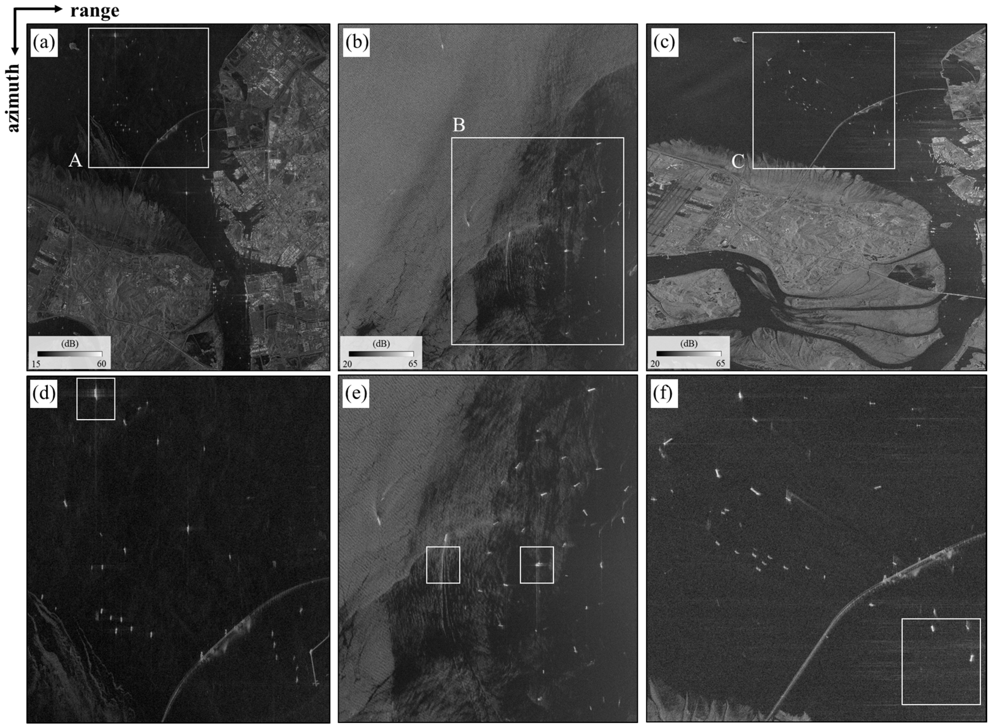
The COSMO-SkyMed and KOMPSAT-5 images were acquired in the single look complex (SLC) format in the StripMap HIMAGE and enhanced standard (ES) modes with horizonal-horizontal (HH) single polarization, respectively, and the TerraSAR-X image was obtained in the SLC format in the StripMap mode with HH and vertical-vertical (VV) dual polarization. The HH polarized TerraSAR-X images were only used for this study. Table 1 presents the detailed image parameters of the test images. Since the TerraSAR-X image was obtained with the dual polarization mode, its nominal azimuth resolution was 2 times lower than the COSMO-SkyMed and KOMPSAT-5 images. The SAR image quality can be measured from the peak side lobe ratio (PSLR) because the PSLR refers to the ability of SAR to identify a weak target in a nearby strong target. PSLR is defined as the ratio of the peak intensity in the main lobe of the impulse response function (IRF) to the peak intensity of the most intense side lobe [27]. The PSLR of the KOMPSAT-5 image was less than -20 dB (Table 1); hence, the KOMPSAT-5 image quality was lower than the quality of the COSMO-SkyMed and TerraSAR-X images. The TerraSAR-X image with a value of less than -25 dB was of higher quality. This indicates that the TerraSAR-X image used for this study had a higher image quality, while it had a lower spatial resolution. Figure 1 shows the test images acquired from the COSMO-SkyMed, Kompsat-5, and TerraSAR-X SAR satellites.
As shown in Figure 1a–c, the ship objects were clearly more visible than the surrounding sea due to the corner reflection effect. The larger the incidence angle was, the larger the brightness difference between ships and sea pixels was. Due to this phenomenon, the sea pixels of the COSMO-SkyMed and TerraSAR-X images were relatively darker than those of the KOMPSAT-5 image, and the contrast between ship and sea brightness values was more pronounced, as seen in Figure 1. This indicates that a larger incidence angle would be helpful for separating ship objects from the sea. In the COSMO-SkyMed image, there are side-lobe effects [28] around some of the ships and wave textures in the background (Figure 1d). In the Kompsat-5 image, there are also strong wave textures, side-lobe effects, and ship wakes (Figure 1e). As the wake was less visible at larger incidence angles [29], some wakes are more observable in the KOMPSAT-5 SAR image than in the other two images. As shown in Figure 1f, there are side-lobe effects and radio frequency (RF) interference in the range direction. The RF interference is caused by the narrow bandwidth and short duration [30]. The phenomena shown in Figure 1d–f could give rise to false alarms, and hence, they have to be mitigated before applying data to machine learning algorithms.
2.2. Methods
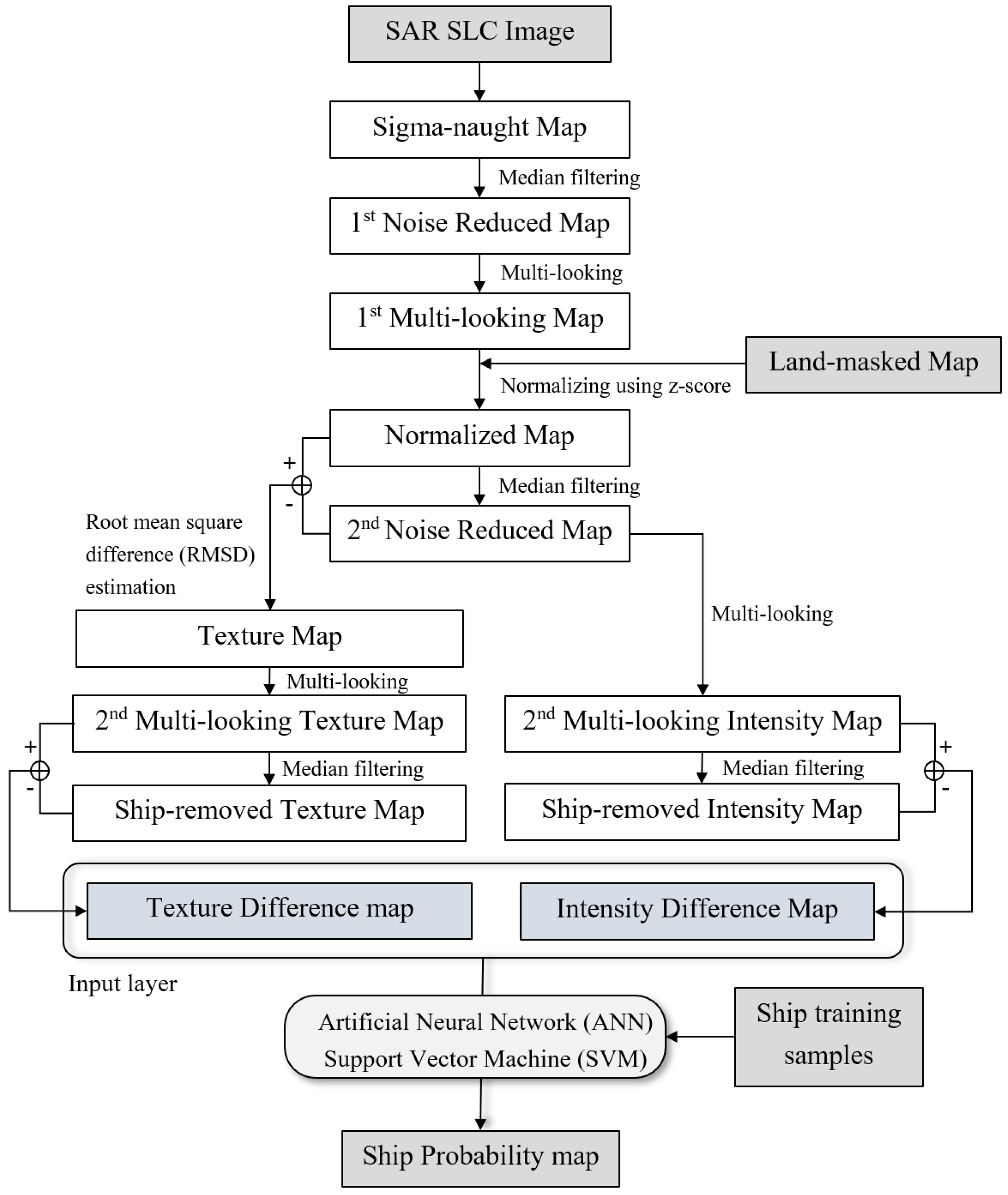
This study aimed to propose an improved ship detection method using machine learning techniques from SAR images. Figure 2 shows the flow of the proposed method. This paper consists of the following three parts: (1) The generation of two input neurons through ship target enhancement; (2) the application of the two input neurons to machine learning approaches including ANN and SVM; and (3) performance validation of the proposed method.
The process of generating the two effective input neurons is divided into two parts. One part has the objective of strengthening the ships and reducing negative effects, such as speckle noise, side-lobe effect, ship wake, wave texture, etc. To meet this goal, the median filter, multi-look processing, and root-mean-square difference calculation are used to mitigate the speckle noise and enhance ship targets in the SAR image. The other part aims to enhance the difference in the pixel values between ship targets and sea. In particular, to achieve a highly accurate ship detection result using a machine learning algorithm, it is very important to generate difference values between ships and the surrounding sea.
The detailed processing steps of the proposed method are as follows:
- (1)
- Generate a sigma-naught image from a SAR SLC image;
- (2)
- Create a first noise-reduced map by using a first median filtering of 7 × 7 kernel size;
- (3)
- Produce a first multi-looking map by 2 × 2 multi-look processing;
- (4)
- Generate a normalized map by using Z-score after masking out land areas;
- (5)
- Create a second noise-reduced map by using second median filtering of 15 × 15 or 19 × 19 kernel sizes;
- (6)
- Produce a textured map through the root-mean-square difference (RMSD) calculation between the normalized and second noise-reduced maps;
- (7)
- Generate second multi-looking intensity and texture maps from the second noise-reduced and texture maps by 2 × 2 multi-look processing, respectively;
- (8)
- Create ship-removed intensity and texture maps from the second multi-looking intensity and texture maps by 51 × 51 median filtering, respectively;
- (9)
- Produce intensity difference maps using the difference between the second multi-looking maps and the ship-removed maps; and
- (10)
- Produce texture difference maps using the scaled difference between the second multi-looking maps and the ship-removed maps.
In this study, the SAR processing was conducted with GAMMA software. The sigma-naught SAR images were also calculated by using the calibration constants given by the header files.
2.2.1. Mitigation of Speckle Noise and Land Masking
Speckle noise is typically present in SAR images. It arises from the random interference between coherent returns that occurs due to the abundant scatterers that are present on a surface [34]. Speckle noise appears as bright and dark pixels that degrade the quality of the SAR image, and it is an obstacle in the detection of targets [35]. Thus, to improve the interpretation of SAR images, speckle noise needs to be reduced. In general, speckle is reduced by the multi-look technique [36] and filtering. The multi-look technique reduces the azimuth and range bandwidths, and thus the speckle noise, but it degrades the image resolution, resulting in the loss of small ship targets if an excessively large look segment is applied [34]. Moreover, the remaining speckle can be addressed using filters [37,38,39]. The median, Kuan, Lee, Gamma, and Frost filters have been used widely, but they have some limitations associated with the degradation of resolution [34]. Therefore, the small multi-look algorithm and a median filter with a small window kernel size were applied to the SLC SAR images to reduce the speckle noise and any other background noise while maintaining the resolution.
It is very important to mask out land areas before detecting ship targets, because numerous false alarms are produced from land areas in SAR images. Many studies have masked out land area by means of the SRTM DEM (Shuttle Radar Topography Mission Digital Elevation Model) [40,41,42], DTM (Digital Terrain Model) [29], or coastline detection [43,44,45,46]. In this test, it was difficult to mask land areas by using an existing DEM because tidal flat areas existed in the COSMO-SkyMed and TerraSAR images. Thus, a coastline detection method was used to mask land areas. The land and ship targets in the SAR images are located on the higher side of the image histogram, whereas the sea clutter is on the lower side. Based on this, the multi-level Otsu method [47] and the morphology technique were used to separate land and sea.
2.2.2. Generation of the Input Layer
After normalizing the first multi-looking map, the median filter is applied to reduce the noise effects by selecting a size equal to about half the average ship size as the median kernel size (Figure 2). For the purpose of mitigating the negative effects and detecting even small ships, the RMSD calculation is performed on the normalized map, and the second noise-reduced map. Through the RMSD calculation, the texture map is generated. In the texture map, even very small ships can be prominent. Thus, the texture map is used as an input neuron to effectively detect most ships in a SAR image.
The median filter is utilized to create two input neurons with enhanced ship targets. When the median window kernel is moving, the center pixel value of the window kernel is changed to the median value of the window kernel pixel values. This characteristic enables the median filter to efficiently mitigate noise. Moreover, the median filter can be used to effectively remove ship targets. If the ship target pixels in an image are not selected as the median value in the window kernel of the median filter, the ship targets will disappear in the image. To prevent this, the kernel size of the median filter used for the ship removal should be determined by considering the sizes of the ship targets, and hence the kernel size should be relatively large. Ship-removed images can be created by using the median filter with a large kernel size, and ship-enhanced images can be generated from the differences before and after the median filtering.
Based on the median filtering, as shown in Figure 2, the intensity difference map is generated by subtracting the ship-removed intensity and texture maps from the second multi-looking intensity, and the texture difference map is created by (i) subtracting the ship-removed intensity and texture maps from the second multi-looking intensity and texture maps and (ii) dividing the subtracted maps by the ship-removed intensity and the texture maps (scaled from 0.01 to 1), respectively. Following the processing, in the intensity difference map, ships have high intensity, and noise such as speckle, side-lobe effect parts, ship wake, and wave texture has low intensity. Even though very small ships have low values in the intensity difference map, this disadvantage is supplemented by the texture difference map.
2.2.3. Artificial Neural Network (ANN)
The artificial neural network (ANN) [48] approach, which is modeled on the human brain system, is a computational mechanism. ANN, a neural network (NN), is composed of many neurons and an activation function for transfer from one neuron to another, similar to the brain’s information delivery system. This is called the multi-layer perceptron (MLP). The MLP is comprised of an input layer, a hidden layer, and an output layer. The input layer and the hidden layer, and the hidden layer and the output layer are connected to each other to form a network [49]. As the neuron is activated by a transmitted signal when the signal is strong enough, the ANN also has an activation function that acts as a threshold. There are many different types of activation functions, such as sigmoid, Tanh, ReLU, Softmax, and others. During the process of training the neural network, weights are found through the activation function and are updated using the most common backpropagation iteration process [50]. A widely used method of updating the weights is the gradient descent method. It is repeated until the slope reaches the minimum value of the function according to the updated weight value. Here, the appropriate learning rate needs to be set so that the slope does not diverge or stop at the non-minimum value.
In this study, MATLAB software was used to execute the ANN algorithm. The two input neurons were selected to be learned with the sigmoid function. Neural networks were iterated during 2000 epochs with a learning rate of 0.01. As a result, four neurons were used in the hidden layer and one linear output layer was created. Table 2 summarizes the parameters used for the ANN algorithm in this study.
2.2.4. Support Vector Machine (SVM)
The support vector machine (SVM) [51] is a supervised learning method that is useful for classifying non-linear data. It can classify data by defining the hyperplane that maximizes the Euclidean distance, called the margin, between the two groups. However, if it is difficult to find a hyperplane that completely separates the two groups while maximizing the margin, there is a way to find the hyperplane while allowing the data to exist in the margin. This is called C-SVC [52]. C is the regularization parameter, and it has an inverse relationship with the margin. Meanwhile, when SVM performs the classification of non-linear data, it takes advantage of the kernel functions. The kernel maps the input data to a higher dimension, and it defines the optimal hyperplane that can separate two or more classes when the margin between the vectors in each class is at the maximum [51]. There are different types of kernel function, such as linear, polynomial, radial basis function (RBF), and sigmoid. In general, the RBF kernel function is the most widely used, because it is known to perform well in a variety of applications [53].
The C-support vector classification (C-SVC) model in the LIBSVM tool [54] provided in the scikit-learn open source Python library was used to carry out the SVM algorithm in this study. To perform an effective SVM method, it needs to select optimal kernel parameters, for example, the margin parameter (C) and kernel width (γ). C defines the cost of C-SVC and γ is calculated as 1 divided by the number of features. Through the grid search with cross-validation, the best pair of (C, γ) is identified. Table 3 presents the kernel function and hyper-parameters used for the SVM process. The radial basis function (RBF) kernel was used identically for all three types of data, and the combination of the library SVM (LIBSVM) hyper-parameters was calculated by grid search with 10-fold cross-validation.
2.2.5. Training and Validation Data
In this test, there were no in-situ data for training and validation. Even though the automatic identification system (AIS) is available, it would have difficulty positioning moving ship targets in the SAR image. If the target has a velocity component, its Doppler shift is changed compared to that from the fixed reflector, because the standard SAR processing method is based on the assumption of a static image or a suspended state of a detected object. Consequently, objects that move linearly in the azimuth direction cause a blurring in the azimuth direction, while objects moving in the range direction are displaced in the azimuth direction [43,55,56]. For this reason, in-situ data for training and validation were automatically generated by a statistical approach. The training data for the machine learning algorithm were set based on a statistical threshold. Ship training samples were extracted from the range of one of the input neurons, intensity difference map, and they were calculated as follows:
where P(i,j) is the pixel value at the range i and azimuth j, TS is the threshold value for the ship samples, MAX(P) is the maximum value of all of the pixels, and Range(P) is the range, which is defined as MAX(P)–MIN(P). The non-ship training samples (PNS) were automatically selected as below:
where TNS is the threshold value for the non-ship samples. The threshold values of (TS, TNS) were selected considering only ship objects as correctly included, because the standard deviation of sea objects has a smaller value and that of ship objects has a higher value.
Thus, the combination of (TS, TNS) of COSMO-SkyMed, KOMPSAT-5, and TerraSAR-X were chosen to be (0.5, 0.2), (0.4, 0.2), and (0.4, 0.3), and as a result, the threshold values for the ship and non-ship samples were (2.03, 0.07), (3.12, −0.19), and (2.24, −0.04), respectively. According to these threshold value combinations, 26 ships for COSMO-SkyMed, 25 ships for KOMPSAT-5, and 41 ships for TerraSAR-X were selected as ship training samples, as shown in Table 4. To validate the performance of the proposed method, real ship targets were identified from the test X-band SAR images through visual analysis. The procedure was carried out in two steps: (i) determination of ship candidates from a SAR image and (ii) the removal of offshore and seaside structures and buoys from the candidates using the Google Earth image. Table 4 summarizes the number of the ground-truth ship targets in the COSMO-SkyMed, KOMPSAT-5, and TerraSAR-X images.
2.2.6. Accuracy Assessment
The statistical threshold value was used to validate results of the ANN and SVM. It was calculated from each ship-probability map histogram. The probability of sea was on the left side and that of the ship was on the right side of the histogram. The threshold value for the ship was obtained from the point where each region intersects. Therefore, the threshold values of the ANN results for COSMO-SkyMed, KOMPSAT-5, and TerraSAR-X were estimated to be 0.74, 0.72, and 0.66, and those of the SVM results of COSMO-SkyMed, KOMPSAT-5, and TerraSAR-X were estimated to be 0.62, 0.71, and 0.65, respectively. When applying the threshold value to the ship-probability map to identify the final ships, the recall, which is a measure of how accurately ship is detected, and the precision, which is a measure of how many objects are detected correctly by the method, were calculated, as shown in Table 4. The recall and precision were calculated as
where is the ground-truth number, is the number of objects detected by the method, and is the number of correctly detected ships in .
Both indexes depend on the thresholds applied and can be expressed in a precision-recall graph to see the performance of the classifier. As the recall and precision have a tradeoff relationship, the better the classifier is, the closer the graph is to the upper right-hand side. Moreover, it is possible to quantitatively compare the classifier by calculating the area under the precision-recall curve, called the average precision (AP).
3. Results
The performance of the proposed method was tested using the three X-band SAR images: COSMO-SkyMed, KOMPSAT-5, and TerraSAR-X. For the test, the intensity images were first generated from the complex SLC data. Since the SAR images follow the Rayleigh distribution, it needed to be changed into the Gaussian distribution. Thus, the sigma-naught maps were created, and the data units were converted into decibels. Then, to reduce the speckle noise, the first median filter with a kernel size of of 7 × 7 was applied to the sigma-naught maps, and then the first multi-looking operation of 2 × 2 was applied. The median filter size and the multi-looking size were determined by considering the spatial resolution to minimize the non-detection of small ships.
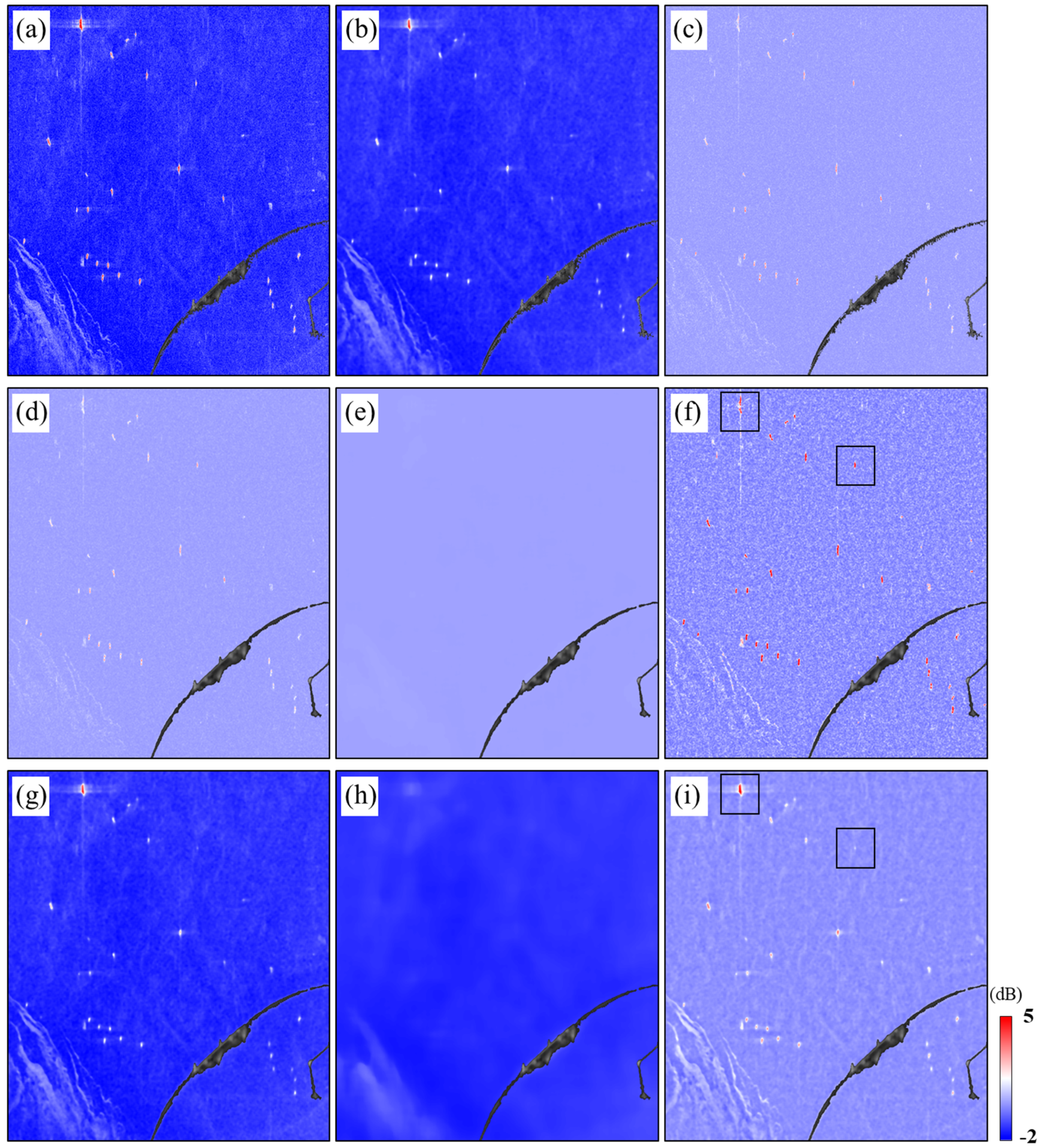
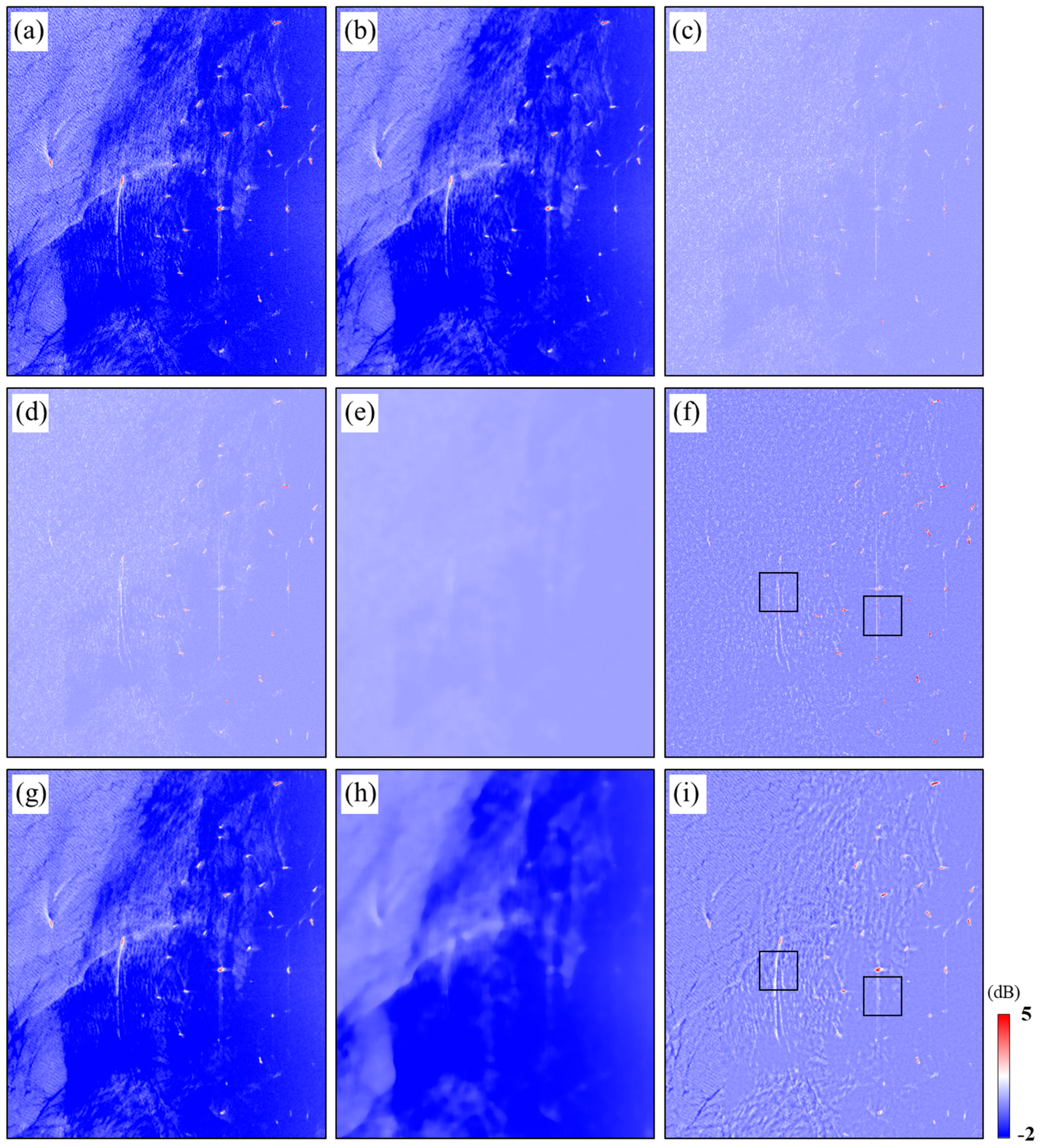
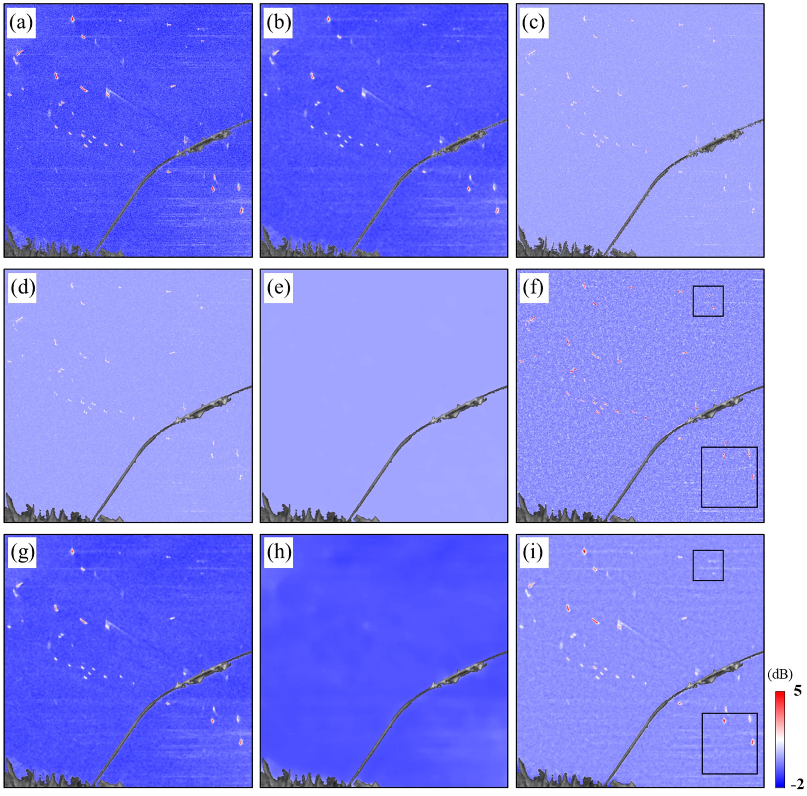
The land masking images were created from the test images with the coastline detection algorithm. However, some of the shallow tidal flats in the COSMO-SkyMed image were classified as sea region in the masking image, and hence, those parts were not masked out, as shown in the lower left part of Figure 3a. After the land areas in the first multi-looking maps had been masked out, the first multi-looking maps were normalized with the z-score, which is calculated from the mean and standard deviation. Then, to generate the second noise reduced maps, the median filter with a kernel size of 15 × 15 was applied to the normalized maps of COSMO-SkyMed and TerraSAR-X, respectively, and the median filter of 19 × 19 was applied to the KOMPSAT-5 normalized map considering the ship target size. The noises in the filtered maps were remarkably reduced, and small bright targets, such as buoys, were erased in the maps, as shown in Figure 3b, Figure 4b and Figure 5b.
The texture maps were created by the RMSD estimation between the normalized maps and the second noise-reduced maps with a 3 × 3 moving window. As shown in Figure 3c, Figure 4c, and Figure 5c, small ships were very clear in the texture maps. In the COSMO-SkyMed texture map, the side-lobe effect and some tidal flats that were not masked out appear weak, and the wave texture of the background is clearly shown in Figure 3c. In the KOMPSAT-5 texture map seen in Figure 4c, ship wake is rather weak, but the side-lobe effect is remarkable. In the case of TerraSAR-X, the ship wake and radio frequency (RF) interference were remarkably reduced (Figure 5c).
To create the second multi-looking texture maps, shown in Figure 3d, Figure 4d, and Figure 5d, the 2 × 2 multi-look operation and 3 × 3 median filter were carried out on the texture maps to reduce the noise effects. Then, the median filter with a kernel size of 51 × 51, which is sufficiently larger than the ship size, was applied to the second multi-looking texture maps, and the ship-removed texture maps were created. The ship targets clearly disappeared in the ship-removed texture maps as shown in Figure 3e, Figure 4e, and Figure 5e. To maximize the difference between ship and sea objects, the texture difference maps were created by (i) subtracting the ship-removed texture maps from the second multi-looking texture maps and (ii) dividing the subtracted maps by the ship-removed texture maps, scaled from 0.01 to 1. Consequently, all of the ship targets became very prominent in the texture difference maps, as can be seen in Figure 3f, Figure 4f, and Figure 5f.
To create the other input neuron, the intensity difference map, a similar process was carried out. The multi-look operation of 2 × 2 was applied to the second noise-reduced map in Figure 3g, Figure 4g, and Figure 5g. The ship-removed intensity maps were generated from the second noise-reduced map by using a median kernel size of 51 × 51. Then, unlike the process for creating the texture difference map, by simply subtracting the ship-removed intensity maps from the second noise-reduced maps, the intensity difference maps were created, as shown in Figure 3i, Figure 4i, and Figure 5i. In the intensity difference maps, larger ships were emphasized, but small ships were not clearly shown. However, the texture difference map made up for this weakness of the intensity difference map. Therefore, these two maps are complementary as well as being a great combination for detecting all ship targets from X-band SAR images.
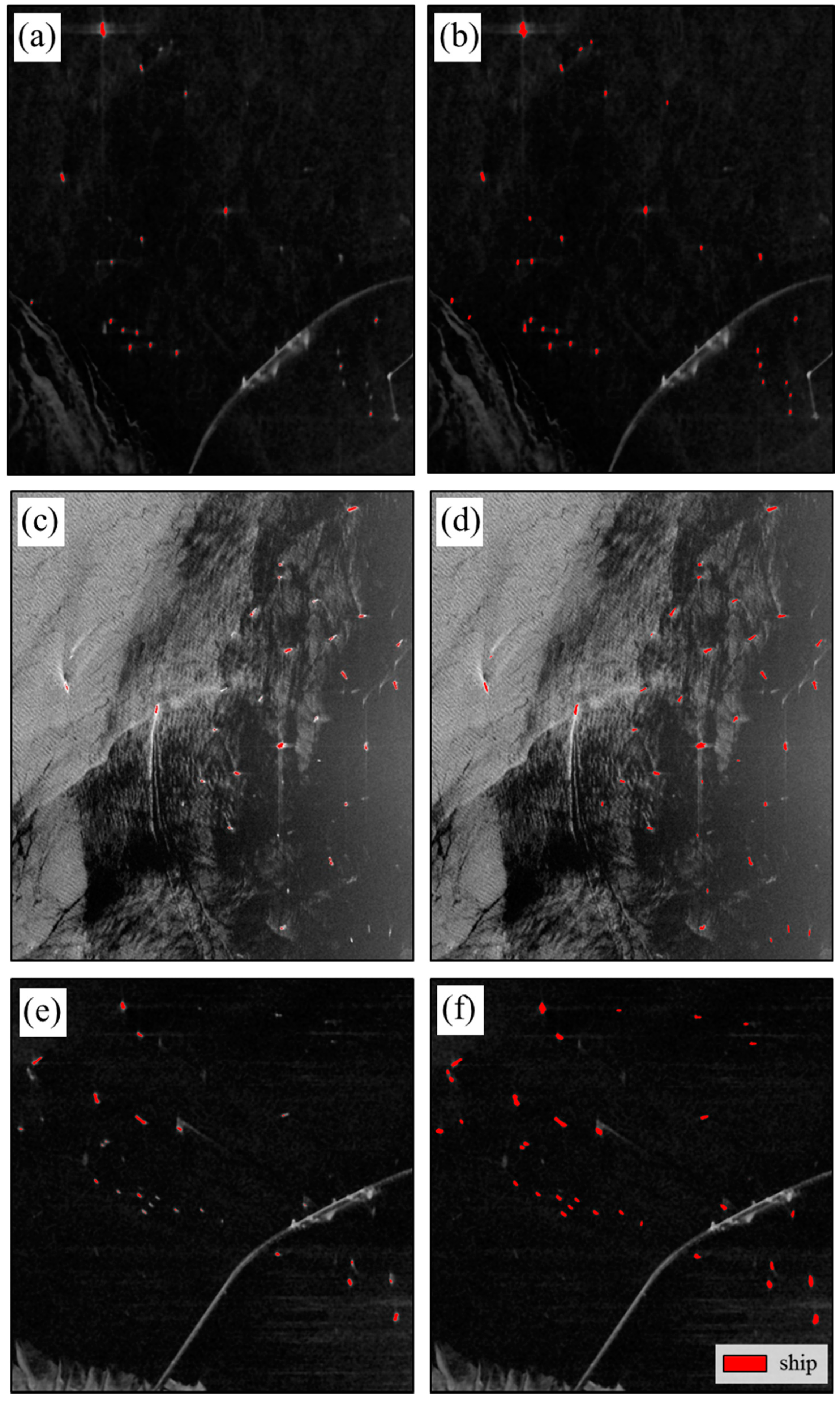
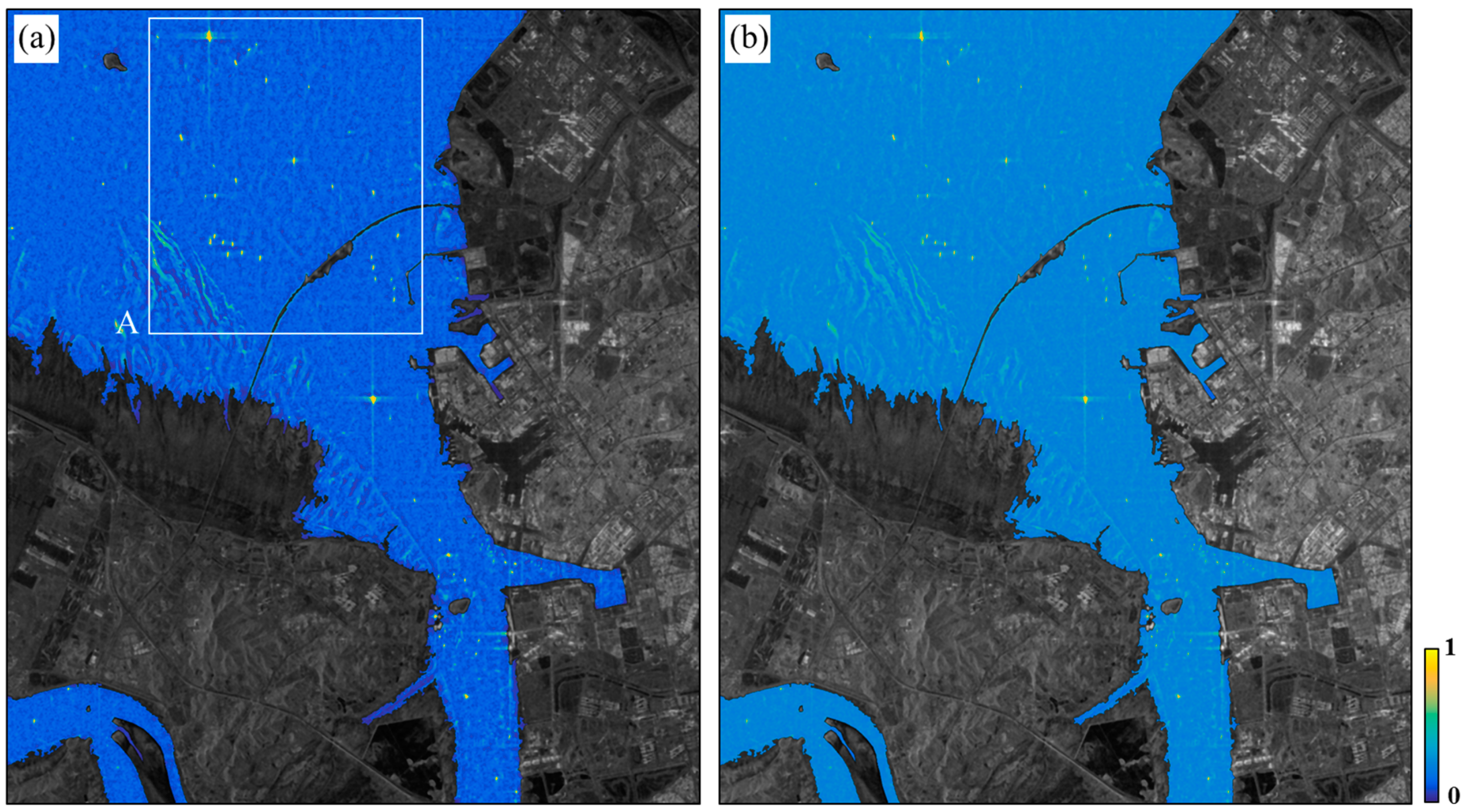
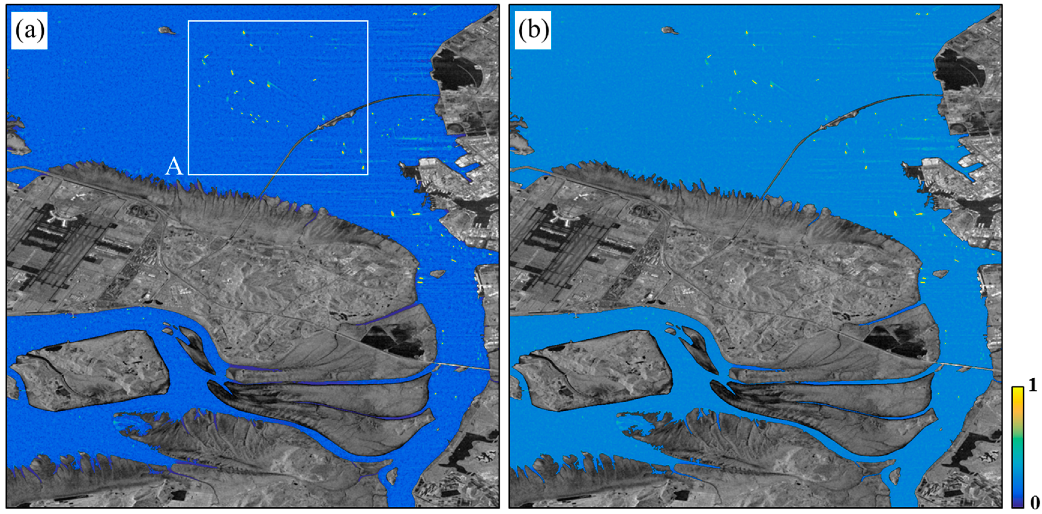
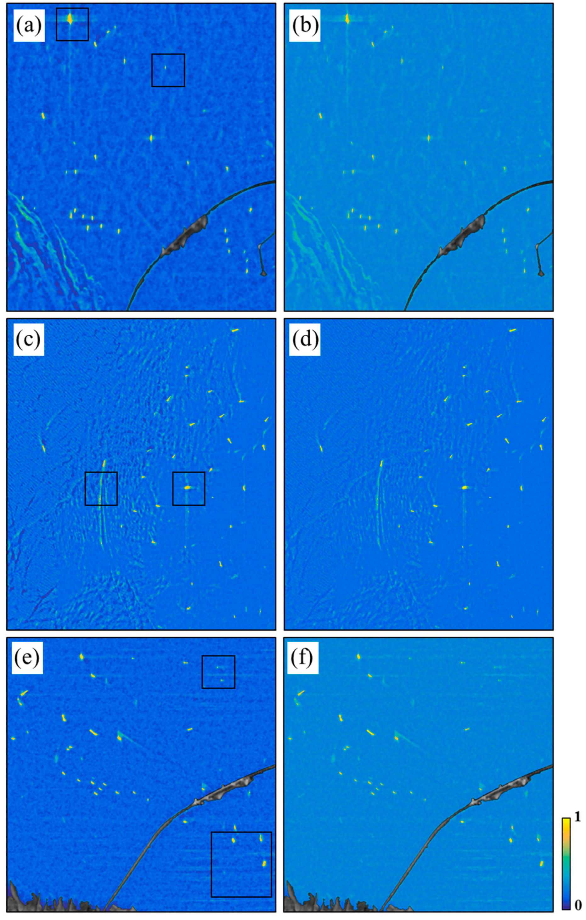
The texture and intensity difference maps generated by the proposed method were applied to the ANN and SVM algorithms as the input neurons. Figure 6a,c,e show the ship objects used to train the neural net of ANN and the classifier of SVM. As mentioned previously, for the training set, the threshold values for the ship samples (TS) in Equation (1) and for the non-ship samples (TNS) in Equation (2) were determined from the intensity difference map considering the statistical distribution of the intensity difference map. Figure 6b,d,f present the ground-truth ship objects in the COSMO-SkyMed, KOMPSAT-5, and TerraSAR-X images, which were extracted by visual analysis. Figure 7, Figure 8 and Figure 9 show the ship-probability maps created from the ANN and SVM approaches. The pixel values in the ship-probability maps are expressed as values from zero to one.
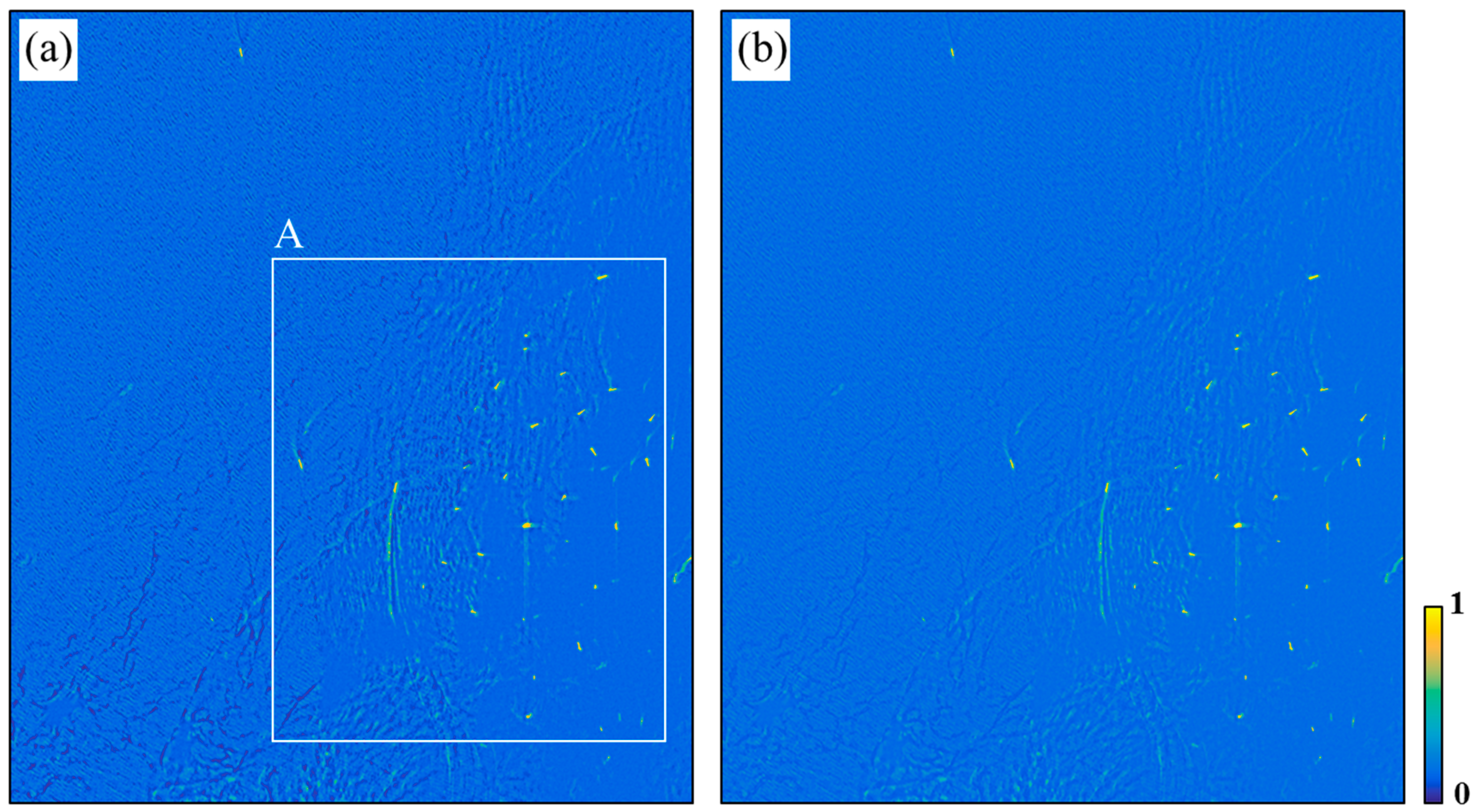
As shown in Figure 10a, in the ANN result of COSMO-SkyMed, the sea objects had a probability from 0.1 to 0.14, and the ship objects had a probability of more than 0.9. The side-lobe effects were from 0.24 to 0.35, and some of the tidal flats that were not masked out had a value of about 0.5, while others had a value of 0.74. In addition, the small ships shown in the black box in Figure 10a had a probability of 0.86 and were easily detected as ship objects. In the SVM result of COSMO-SkyMed (see Figure 10b), the probability of the sea objects increased to 0.28, while the probability of ship targets was slightly lower than the probability shown by the ANN result. Therefore, the threshold had a lower value in the results of the ANN than in the SVM results. Thus, all except three ship objects were found, but the number of false positives increased where an oil fence occurred.
In the case of the ANN result of KOMPSAT-5, shown in Figure 10c, the probability values in the ship objects were about 0.9 and the probability values in the sea objects, including the wave texture, were as low as about 0.2. The side-lobe effect was less than 0.3, but some parts of the ship wake were higher than 0.75. Figure 10d shows the SVM results for KOMPSAT-5. Some parts of the ship wake were about 0.76, and hence they were detected as false alarms. In the ANN analysis of TerraSAR-X, the sea objects had probability values from 0.1 to 0.15 while those of the ship objects were from 0.85 to 0.92 (see Figure 10e). The RF interference part had a probability of about 0.5. The small ships shown in the black box of Figure 10e had a high probability of 0.80. In both the ANN and SVM results of TerraSAR-X, the RF interference effects had a low probability, and there were no false detections from the effects (see Figure 10e,f).
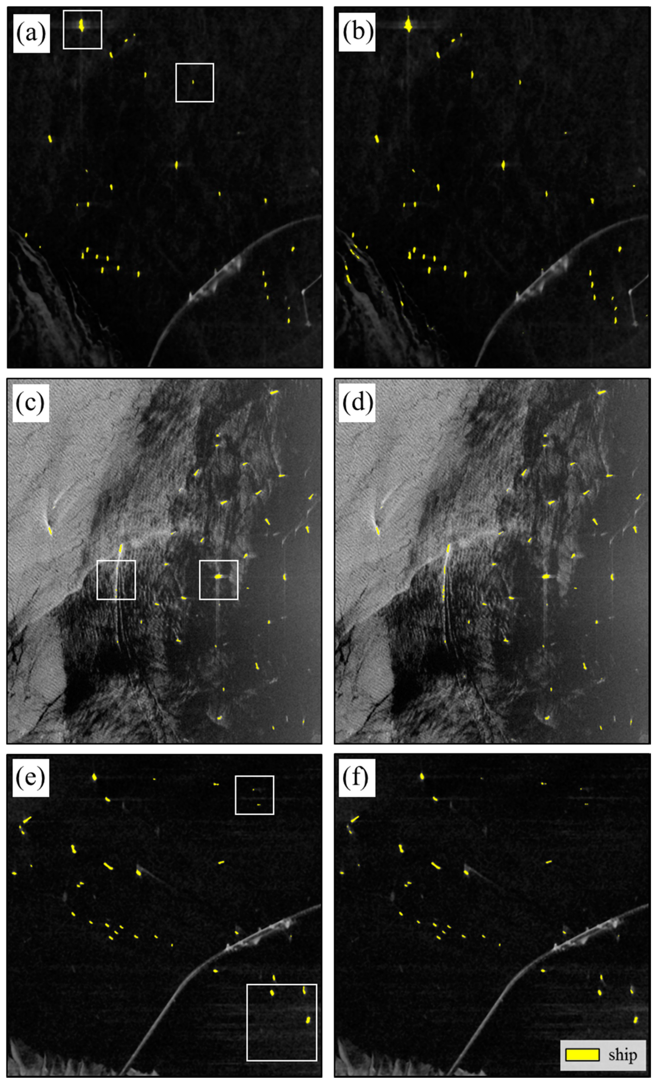
Based on a visual analysis, a total number of 71 ships were found in the COSMO-SkyMed images. When the threshold value of 0.74 was imposed on the COSMO-SkyMed ANN probability map, 63 ship objects were detected; 59 ship objects among the detected ship objects were real ships (Figure 11a). The threshold value of 0.62 was used for the COSMO-SkyMed SVM probability map; 79 ship objects were detected and 68 ship objects among the detected ships were real, as seen in Figure 11b. Eleven ships were not detected in the COSMO-SkyMed ANN results and three were not detected in the SVM results. Most of the non-detected ship objects had a probability of 0.5 to 0.72. Most of the false positives in the COSMO-SkyMed came from the tidal flats areas that were not masked out, but some of them arose from floating marine objects, for example, oil fences, buoys, and dolphins. The (recall, precision) results for the COSMO-SkyMed ANN and SVM were (83.10%, 93.65%) and (95.77%, 86.08%), respectively. These results mean (i) that 95.77% of all the ships were found with the SVM, but 13.92% of the detected ships were false positives; and (ii) that 83.10% of all real ships were detected with the ANN, but 6.35% of the detected ships were false positives.
In the case of KOMPSAT-5, 40 real ships were present in the image. The optimal threshold value was determined to be 0.72 with ANN, and hence, 42 ship objects were detected and 38 among the objects were correctly detected (Figure 11c). With the SVM, when the optimal threshold of 0.71 was used, 40 ship objects were detected and 39 among those detected were real (Figure 11d). Consequently, the (recall, precision) results of the KOMPSAT-5 ANN and SVM were (95.00%, 90.48%) and (97.50%, 97.50%), respectively. Most false detections in the KOMPSAT-5 occurred due to the ship wake. The ship wake was weakened in the intensity difference map, while the ship wake was relatively visible in the texture difference map.
For the case of the TerraSAR-X images, 88 real ships were present in the image. When the ANN was applied to the TerraSAR-X images, 92 ship objects and 81 ship objects among the detected were real (Figure 11e). The optimal threshold value was 0.66 with the ANN. When the SVM was applied to the TerraSAR-X images, 90 ship objects were detected and 80, among the detected objects, were identified as real ships (Figure 11f). In this process, the optimal threshold was 0.65. The (recall, precision) of the ANN and SVM results were (92.05%, 88.04%), (90.91%, 88.89%), respectively. The ship objects of seven to eight were not detected in the ANN and SVM results for the TerraSAR-X images. Most of the non-detected ships were small—about six pixels in length. Moreover, most false alarms occurred from floating marine objects, as in the case of the COSMO-SkyMed results, and from some pipelines.
The results from COSMO-SkyMed, KOMPSAT-5, and TerraSAR-X are summarized in Table 5. In the COSMO-SkyMed and KOMPSAT-5 test images, the SVM approach was better than the ANN, while the two approaches performed similarly in the TerraSAR-X test image. The results for the TerraSAR-X images were also lower than those for the COSMO-SkyMed and KOMPSAT-5 images. However, it should be noted that the spatial resolution of the TerraSAR-X image is two times lower than those of the COSMO-SkyMed and KOMPSAT-5 images, and the image quality of the TerraSAR-X is higher than the other images. With TerraSAR-X, since the number of non-detected ship objects was very small, the degraded result from TerraSAR-X could have been due to the low spatial resolution.
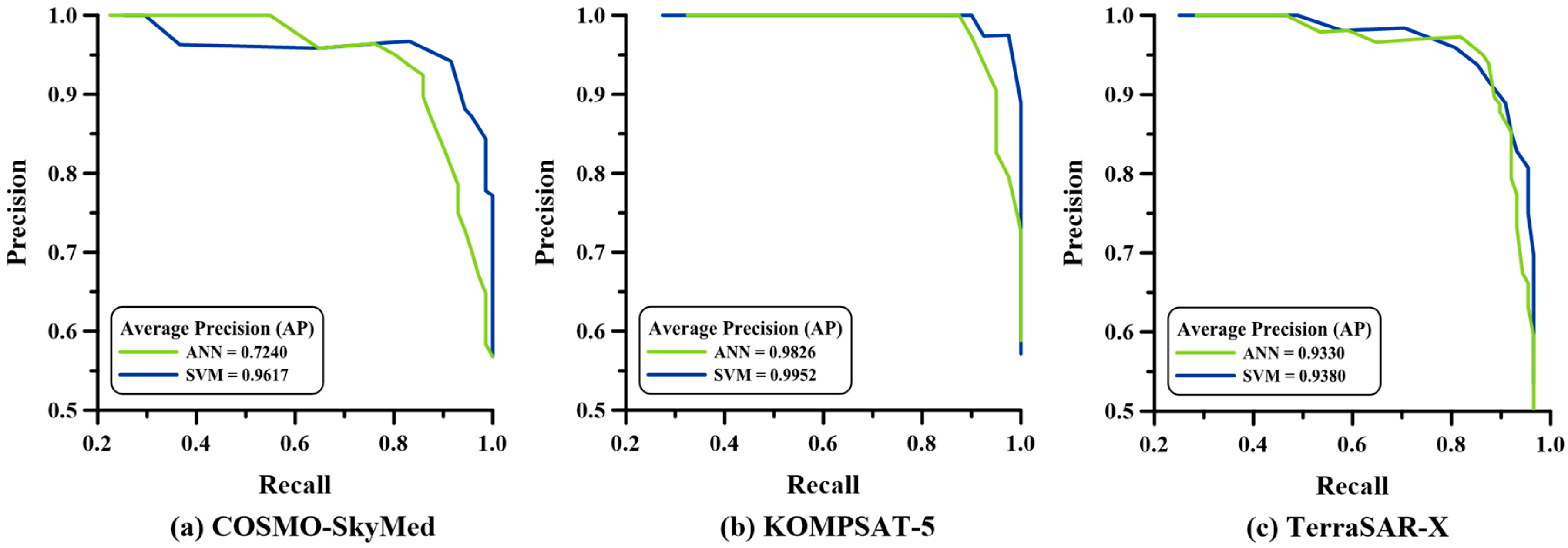
Figure 12 presents the recall-precision curve of the COSMO-SkyMed, KOMPSAT-5, and TerraSAR-X results. The average precision (AP) was calculated as a comparison between the ANN and SVM approaches. First of all, in the case of the COSMO-SkyMed images, the AP values of ANN and SVM were about 0.724 and 0.962, respectively. This means that the use of SVM on the COSMO-SkyMed images gave a better performance than the ANN. In KOMPSAT-5, the AP values of the ANN and SVM results were about 0.983 and 0.995, respectively, and the ANN and SVM results from TerraSAR-X had AP values of about 0.933 and 0.938, respectively. For the KOMPSAT-5 and TerraSAR-X images, the AP values of the ANN and SVM results were good as well as being very similar, but the SVM method gave slightly better results than the ANN.
4. Discussion
In this study, we tested how an optimal input layer can be formed when machine learning techniques, such as ANN and SVM, are used to detect ships from X-band SAR images. The optimal input layer was composed of two input neurons: (1) an intensity difference map and (2) a texture difference map. In this study, we proposed the use of the SAR processing procedure to generate the intensity difference map and texture difference map. As shown in Figure 2, the detailed procedure was conducted by image processing, including multi-looking, median filtering, and texture extraction. As seen in Figure 3, Figure 4 and Figure 5, the two maps clearly enhanced the ship targets and reduced the number of false alarms. However, when the texture difference map was generated, the buoys and small bright targets were emphasized, hence increasing the false alarm rate. Since the COSMO-SkyMed and TerraSAR-X images were acquired in the coastal area, buoys, and small bright targets were present in the images, and hence the number of false alarms in those images was greater than in the KOMPSAT-5 image. Moreover, it was noted that the optimal determination of the filter kernel size is very important to improve the detection efficiency. We determined the optimal filter sizes for the intensity and texture difference maps using the three test images through an empirical approach. However, the optimal filter size can change according to the image quality and spatial resolution.
As mentioned previously, the intensity and texture difference maps were successfully applied to the ship detection using the ANN and SVM algorithms. The detection results from the COSMO-SkyMed, KOMPSAT-5, and TerraSAR-X test images show that their precisions were larger than 86% as well as their recalls were more than 90% except the COSMO-SkyMed ANN result. It was reported that the recalls of the standard and intensity-space (IS) domain CFAR algorithms using TerraSAR-X images were respectively about 68% and 83% [57]. When a contextual region-based convolutional neural network (CNN) approach proposed by Reference [21] was applied to the Sentinel-1 C-band SAR data, the achieved recall was about 87% with the false alarm of about 13%. In the CNN result, small ships were not considered due to the low spatial resolution of the Sentinel-1 interferometric wide swath (IW) mode, as well as most missing ships were caused by the SAR imaging characteristics such as the side lobe effects, speckle noise, and ghost phenomenon, etc. We can conclude that the achieved detection performance of the proposed method is better than the standard and IS domain CFAR algorithms and the CNN approach, if it is assumed that the ship detection tests were similarly performed. The improvement would be because the intensity and texture difference maps, which were used as the input neurons of the ANN and SVM approaches, clearly enhanced the ship targets as well as remarkably reducing the noise effects. It means that the proposed method is appropriate for the effective detection of ship targets. Among the test images, the detection performance of KOMPSAT-5 was higher than that of COSMO-SkyMed and TerraSAR-X. That is, the precision from KOMPSAT-5 was higher while the false detection rate was lower. The low false detection rate occurred because buoys and small bright targets in the KOMPSAT-5 test image are almost nonexistent, although high sea waves do exist in the image. The high precision achieved was also because the KOMPSAT-5 test image does not include smaller ships. Since the COSMO-SkyMed and TerraSAR-X test images include buoys and small bright targets, their precisions were lower than the KOMPSAT-5 test image. Thus, we cannot conclude from the results that the detection performance from KOMPSAT-5 images was higher than the detection performance from COSMO-SkyMed and TerraSAR-X images due to the buoys and small bright targets in the COSMO-SkyMed and TerraSAR-X images. The results indicate that the detection performance of the proposed method was not largely different among the COSMO-SkyMed, KOMPSAT-5, and TerraSAR-X images. In the COSMO-SkyMed test, the SVM algorithm performed better than the ANN. This is because the threshold value was not optimally determined. In the ANN, the optimal threshold value must be lower than 0.74. The ANN method only detected 59 ship targets from 71 true ship targets. While the false detection rate of SVM was higher than that of ANN, the SVM identified 68 ships from 71 true ships because the threshold value was optimally determined. In the KOMPSAT-5 test, the SVM performed slightly better than the ANN. The SVM method detected 39 ships among 40 true ships. On the other hand, the ANN results were similar to the SVM results in the TerraSAR-X test. This may indicate that the threshold value determination from SVM ship-probability maps is easier than in the ANN ship-probability maps. To compare the performances of the ANN and SVM, a recall-precision curve was derived, and AP values were calculated. The AP values of the ANN and SVM results were (0.724, 0.962), (0.983, 0.995), and (0.933, 0.938) in the COSMO-SkyMed, KOMPSAT-5, and TerraSAR-X images, respectively. The results show that the SVM performed better than the ANN.
5. Conclusions
We proposed an effective ship detection method using machine learning from X-band SAR images. It is a fact that machine learning results depend strongly on the composition of the input layer and the training data. Here, two input layers were generated for the purpose of obtaining highly accurate ship detection results from high-resolution X-band SAR images including the COSMO-SkyMed, KOMPSAT-5, and TerraSAR-X images. The two input neurons were generated to (i) emphasize ship targets from sea and (ii) mitigate the negative effects that cause false detections, e.g., speckle noise, side-lobe effects, ship wake, etc. To generate the input neurons, the median filter, multi-look operation and RMSD calculation were used to generate the input neurons. After the input neurons were generated, including the intensity and texture difference maps, they were successfully applied to the ANN and SVM approaches, respectively. Consequently, ship-probability maps were created by the ANN and SVM approaches, respectively. Finally, ship detection was performed by determining an optimal threshold value from the probability map. For the performance validation, ship objects were identified by visual analysis, and the (recall, precision) and AP values were calculated. The recall values estimated from the ANN approach were about 83.1%, 95.0%, and 92.1% for the COSMO-SkyMed, KOMPSAT-5, and TerraSAR-X images, respectively, and the recall values from the SVM approach were about 95.8%, 95.0%, and 90.9%, respectively. The precision values estimated from the ANN and SVM approaches were about 93.7% and 86.1% for the COSMO-SkyMed image, about 90.48% and 97.50% for the KOMPSAT-5 image, and about 88.04% and 88.89% for the TerraSAR-X image, respectively. The AP values with the ANN and SVM were about 0.724 and 0.962 in the COSMO-SkyMed image, about 0.983 and 0.995 in the KOMPSAT-5 image, and about 0.933 and 0.938 in the TerraSAR-X image. The KOMPSAT-5 results were clearly better than the COSMO-SkyMed and TerraSAR-X results. However, it cannot be concluded from the results that the detection performance from KOMPSAT-5 images was higher than the detection performance from COSMO-SkyMed and TerraSAR-X images. This is because the KOMPSAT-5 test image does not include buoys and small bright targets, while the COSMO-SkyMed and TerraSAR-X test images do include them. In particular, for the TerraSAR-X image, the precision and recall were lower than for the COSMO-SkyMed and KOMPSAT-5 images. The is due to the lower spatial resolution of the TerraSAR-X image. In the TerraSAR-X results, most small ships were not detected. If a single-polarized TerraSAR-X image was used, the detection performance from the TerraSAR-X image might be best because the spatial resolution of the TerraSAR-X image is similar to the COSMO-SkyMed and KOMPSAT-5 images and the image quality of the TerraSAR-X is much higher than the other images. From the results, it was demonstrated that the proposed method is remarkably effective for detecting ships from X-band SAR images. Moreover, the proposed method could be applied by adjusting the parameter values of the filtering technique according to the SAR image quality.
Author Contributions
Conceptualization, H.-S.J.; methodology, J.-I.H. and H.-S.J.; software, J.-I.H.; validation, J.-I.H. and H.-S.J.; formal analysis, J.-I.H. and H.-S.J.; investigation, J.-I.H., H.-S.J.; writing–original draft preparation, J.-I.H.; writing—review & editing, H.-S.J.; visualization, J.-I.H.; supervision, H.-S.J.
Funding
This work was supported by a National Research Foundation of Korea (NRF) grant funded by the government of Korea (MSIT) (No. NRF-2018M1A3A3A02066008).
Acknowledgments
The TerraSAR-X data used in this study were provided by the German Aerospace Center (DLR) via the proposal (LAN2935).
Conflicts of Interest
The authors declare no conflict of interest.
References
- Khesali, E.; Enayati, H.; Modiri, M.; Aref, M.M. Automatic ship detection in Single-Pol SAR Images using texture features in artificial neural networks. Int. Arch. Photogramm. Remote. Sens. Spat. Inf. Sci. 2015, 40, 395–399. [Google Scholar] [CrossRef]
- Franceschetti, G.; Lanari, R. Synthetic Aperture Radar Processing; CRC press: Boca Raton, FL, USA, 2018; ISBN 0-8493-7899-0. [Google Scholar]
- Askari, F.; Zerr, B. Automatic Approach to Ship Detection in Spaceborne Synthetic Aperture Radar Imagery: An Assessment of Ship Detection Capability Using RADARSAT; Technical Report SACLANTCEN-SR-338; SACLANT Undersea Research Centre: La Spezia, Italy, 2000. [Google Scholar]
- Corbane, C.; Najman, L.; Pecoul, E.; Demagistri, L.; Petit, M. A complete processing chain for ship detection using optical satellite imagery. Int. J. Remote Sens. 2010, 31, 5837–5854. [Google Scholar] [CrossRef] [Green Version]
- Zhu, C.; Zhou, H.; Wang, R.; Guo, J. A novel hierarchical method of ship detection from spaceborne optical image based on shape and texture features. IEEE Trans. Geosci. Remote Sens. 2010, 48, 3446–3456. [Google Scholar] [CrossRef]
- Shi, Z.; Yu, X.; Jiang, Z.; Li, B. Ship detection in high-resolution optical imagery based on anomaly detector and local shape feature. IEEE Trans. Geosci. Remote Sens. 2014, 52, 4511–4523. [Google Scholar] [CrossRef]
- Corbane, C.; Marre, F.; Petit, M. Using SPOT-5 HRG data in panchromatic mode for operational detection of small ships in tropical area. Sensors 2008, 8, 2959–2973. [Google Scholar] [CrossRef] [PubMed]
- Corbane, C.; Pecoul, E.; Demagistri, L.; Petit, M. Fully automated procedure for ship detection using optical satellite imagery. In Proceedings of the SPIE 7150, Remote Sensing of Inland, Coastal, and Oceanic Waters, Noumea, New Caledonia, 17–21 November 2008. [Google Scholar] [CrossRef]
- Jubelin, G.; Khenchaf, A. Multiscale algorithm for ship detection in mid, high and very high resolution optical imagery. In Proceedings of the 2014 IEEE Geoscience and Remote Sensing Symposium (IGARSS), Quebec City, QC, Canada, 13–18 July 2014. [Google Scholar] [CrossRef]
- di Bisceglie, M.; Galdi, C. CFAR detection of extended objects in high-resolution SAR images. IEEE Trans. Geosci. Remote Sens. 2005, 43, 833–843. [Google Scholar] [CrossRef]
- Gao, G. A parzen-window-kernel-based CFAR algorithm for ship detection in SAR images. IEEE Geosci. Remote Sens. Lett. 2011, 8, 557–561. [Google Scholar] [CrossRef]
- Habib, M.A.; Barkat, M.; Aissa, B.; Denidni, T.A. Ca-cfar detection performance of radar targets embedded in “non centered chi-2 gamma” clutter. Electromagn. Res. 2008, 88, 135–148. [Google Scholar] [CrossRef]
- Cui, Y.; Zhou, G.; Yang, J.; Yamaguchi, Y. On the iterative censoring for target detection in SAR images. IEEE Geosci. Remote. Sens. Lett. 2011, 8, 641–645. [Google Scholar] [CrossRef]
- Lee, Y.K.; Kim, S.W.; Ryu, J.H. Report of Wave Glider Detecting by KOMPSAT-5 Spotlight Mode SAR Image. Korean J. Remote. Sens. 2018, 34, 431–437. [Google Scholar] [CrossRef]
- Liu, C.; Vachon, P.; Geling, G. Improved ship detection with airborne polarimetric SAR data. Can. J. Remote Sens. 2005, 31, 122–131. [Google Scholar] [CrossRef]
- Hannevik, T.N.A. Multi-channel and multi-polarisation ship detection. In Proceedings of the 2012 IEEE International Geoscience and Remote Sensing Symposium (IGARSS), Munich, Germany, 22–27 July 2012. [Google Scholar]
- Gao, G.; Shi, G.; Zhou, S. Ship detection in high-resolution dual-polarization SAR amplitude images. Int. J. Antennas Propag. 2013, 2013. [Google Scholar] [CrossRef]
- Crisp, D.J. A ship detection system for RADARSAT-2 dual-pol multi-look imagery implemented in the ADSS. In Proceedings of the 2013 International Conference on Radar (Radar), Adelaide, Australia, 9–12 September 2013. [Google Scholar]
- Wei, J.; Li, P.; Yang, J.; Zhang, J.; Lang, F. A New Automatic Ship Detection Method Using L -Band Polarimetric SAR Imagery. IEEE J. Sel. Top. Appl. Earth Obs. 2014, 7, 1383–1393. [Google Scholar] [CrossRef]
- Zakhvatkina, N.; Korosov, A.; Muckenhuber, S.; Sandven, S.; Babiker, M. Operational algorithm for ice–water classification on dual-polarized RADARSAT-2 images. Cryosphere 2017, 11, 33. [Google Scholar] [CrossRef]
- Kang, M.; Ji, K.; Leng, X.; Lin, Z. Contextual region-based convolutional neural network with multilayer fusion for SAR ship detection. Remote Sens. 2017, 9, 860. [Google Scholar] [CrossRef]
- Wagner, S.A. SAR ATR by a combination of convolutional neural network and support vector machines. IEEE Trans. Aerosp. Electron. Syst. 2016, 52, 2861–2872. [Google Scholar] [CrossRef]
- Bentes, C.; Velotto, D.; Tings, B. Ship Classification in TerraSAR-X Images with Convolutional Neural Networks. IEEE J. Ocean. Eng. 2017, 43, 258–266. [Google Scholar] [CrossRef]
- Hwang, J.I.; Chae, S.H.; Kim, D.; Jung, H.S. Application of Artificial Neural Networks to Ship Detection from X-Band Kompsat-5 Imagery. Appl. Sci. 2017, 7, 961. [Google Scholar] [CrossRef]
- Mas, J.F.; Flores, J.J. The application of artificial neural networks to the analysis of remotely sensed data. Int. J. Remote Sens. 2008, 29, 617–663. [Google Scholar] [CrossRef]
- Kavzoglu, T. Increasing the accuracy of neural network classification using refined training data. Environ. Model. Softw. 2009, 24, 850–858. [Google Scholar] [CrossRef]
- Eineder, M.; Fritz, T.; Mittermayer, J.; Roth, A.; Boerner, E.; Breit, H. TerraSAR-X Ground Segment, Basic Product Specification Document; Cluster Applied Remote Sensing (Caf): Oberpfaffenhofen, Germany, 2008. [Google Scholar]
- Martinez, A.; Marchand, J.L. SAR image quality assessment. Rev. De Teledeteccin 1993, 2, 12–18. [Google Scholar]
- Eldhuset, K. An automatic ship and ship wake detection system for spaceborne SAR images in coastal regions. IEEE Trans. Geosci. Remote Sens. 1996, 34, 1010–1019. [Google Scholar] [CrossRef]
- Reigber, A.; Ferro-Famil, L. Interference suppression in synthesized SAR images. IEEE Geosci. Remote Sens. Lett. 2005, 2, 45–49. [Google Scholar] [CrossRef]
- ISA. COSMO-SkyMed Mission and Products Description; Italian Space Agency (ISA): Rome, Italy, 31 May 2016.
- KARI. KOMPSAT-5 PRODUCT SPECIFICATIONS Standard Products Specifications, Korea Aerospace Research Institute (KARI); KARI: Daejeon, Korea, July 2015. [Google Scholar]
- DLR. TerraSAR-X Ground Segment Basic Product Specification Document; The German Aerospace Center (DLR): Cologne, Germany, 24 February 2008.
- Gagnon, L.; Jouan, A. Speckle filtering of SAR images: A comparative study between complex-wavelet-based and standard filters. In Proceedings of the SPIE, Wavelet Applications in Signal and Image Processing V, Optical Science, Engineering and Instrumentation, San Diego, CA, USA, 30 July–1 August 1997; Volume 3169, pp. 80–92. [Google Scholar] [CrossRef]
- Sheng, Y.; Xia, Z.-G. A comprehensive evaluation of filters for radar speckle suppression. In Proceedings of the 1996 International Geoscience and Remote Sensing Symposium, Remote Sensing for a Sustainable Future, Lincoln, NE, USA, 27–31 May 1996. [Google Scholar]
- Lee, J.-S.; Grunes, M.R.; De Grandi, G. Polarimetric SAR speckle filtering and its implication for classification. IEEE Trans. Geosci. Remote Sens. 1999, 37, 2363–2373. [Google Scholar] [CrossRef]
- Lee, J.-S. Digital image enhancement and noise filtering by use of local statistics. IEEE Trans. Pattern Anal. Mach. Intell. 1980, 2, 165–168. [Google Scholar] [CrossRef] [PubMed]
- Frost, V.S.; Stiles, J.A.; Shanmugan, K.S.; Holtzman, J.C. A model for radar images and its application to adaptive digital filtering of multiplicative noise. IEEE Trans. Pattern Anal. Mach. Intell. 1982, 4, 157–166. [Google Scholar] [CrossRef] [PubMed]
- Lopes, A.; Nezry, E.; Touzi, R.; Laur, H. Structure detection and statistical adaptive speckle filtering in SAR images. Int. J. Remote Sens. 1993, 14, 1735–1758. [Google Scholar] [CrossRef]
- Saur, G.; Estable, S.; Zielinski, K.; Knabe, S.; Teutsch, M.; Gabel, M. Detection and classification of man-made offshore objects in terrasar-x and rapideye imagery: Selected results of the demarine-deko project. In Proceedings of the IEEE OCEANS 2011, Santander, Spain, 6–9 June 2011. [Google Scholar]
- Hwang, J.; Kim, D.; Jung, H.S. An efficient ship detection method for KOMPSAT-5 synthetic aperture radar imagery based on adaptive filtering approach. Korean J. Remote Sens. 2017, 33, 89–95. [Google Scholar] [CrossRef]
- Kim, S.W.; Kim, D.H.; Lee, Y.K. Operational Ship Monitoring Based on Integrated Analysis of KOMPSAT-5 SAR and AIS Data. Korean J. Remote Sens. 2018, 34, 327–338. [Google Scholar] [CrossRef]
- Brusch, S.; Lehner, S.; Fritz, T.; Soccorsi, M.; Soloviev, A.; van Schie, B. Ship surveillance with TerraSAR-X. IEEE Trans. Geosci. Remote Sens. 2011, 49, 1092–1103. [Google Scholar] [CrossRef]
- Ao, W.; Xu, F.; Li, Y.; Wang, H. Detection and Discrimination of Ship Targets in Complex Background From Spaceborne ALOS-2 SAR Images. IEEE J. Sel. Top. Appl. Earth Obs. 2018, 11, 536–550. [Google Scholar] [CrossRef]
- Margarit, G.; Tabasco, A. Ship classification in single-pol SAR images based on fuzzy logic. IEEE Trans. Geosci. Remote Sens. 2011, 49, 3129–3138. [Google Scholar] [CrossRef]
- Bae, J.; Yang, C.S. Land Masking Methods of Sentinel-1 SAR Imagery for Ship Detection Considering Coastline Changes and Noise. Korean J. Remote Sens. 2017, 33, 437–444. [Google Scholar] [CrossRef]
- Liao, P.-S.; Chen, T.-S.; Chung, P.-C. A fast algorithm for multilevel thresholding. J. Inf. Sci. Eng. 2001, 17, 713–727. [Google Scholar]
- McCulloch, W.S.; Pitts, W. A logical calculus of the ideas immanent in nervous activity. Bull. Math. Biophys. 1943, 5, 115–133. [Google Scholar] [CrossRef]
- Jain, A.K.; Mao, J.; Mohiuddin, K.M. Artificial neural networks: A tutorial. Computer 1996, 29, 31–44. [Google Scholar] [CrossRef]
- Basheer, I.A.; Hajmeer, M. Artificial neural networks: Fundamentals, computing, design, and application. J. Microbiol. Methods 2000, 43, 3–31. [Google Scholar] [CrossRef]
- Cortes, C.; Vapnik, V. Support-vector networks. Mach. Learn. 1995, 20, 273–297. [Google Scholar] [CrossRef] [Green Version]
- Chen, P.H.; Lin, C.J.; Schölkopf, B. A tutorial on ν-support vector machines. Appl. Stoch. Model. Bus. Ind. 2005, 21, 111–136. [Google Scholar] [CrossRef]
- Hsu, C.W.; Chang, C.C.; Lin, C.-J. A Practical Guide to Support Vector Classification. 2003. Available online: https://bit.ly/2QBdXU8 (accessed on 13 November 2018).
- Chang, C.-C.; Lin, C.-J. Libsvm: A library for support vector machines. ACM Trans. Intell. Syst. Technol. 2011, 2, 1–27. [Google Scholar] [CrossRef]
- Kirscht, M. Detection and imaging of arbitrarily moving targets with single-channel SAR. In Proceedings of the IEE Radar, Sonar and Navigation, Edinburgh, UK, 15–17 October 2002; Volume 150, pp. 7–11. [Google Scholar] [CrossRef]
- Osman, H.; Blostein, S.D. Probabilistic winner-take-all segmentation of images with application to ship detection. IEEE Trans. Syst. Man Cybern. B Cybern. 2000, 30, 485–490. [Google Scholar] [CrossRef] [PubMed] [Green Version]
- Wang, C.; Bi, F.; Zhang, W.; Chen, L. An Intensity-Space Domain CFAR Method for Ship Detection in HR SAR Images. IEEE Geosci. Remote. Sens. Lett. 2017, 14, 529–533. [Google Scholar] [CrossRef]
Figure 1.
Multi-looking images obtained by (a) COSMO-SkyMed; (b) KOMPSAT-5; and (c) TerraSAR-X satellite SAR sensors and (d–f) enlargements of boxes A to C in (a–c), respectively.
Figure 1.
Multi-looking images obtained by (a) COSMO-SkyMed; (b) KOMPSAT-5; and (c) TerraSAR-X satellite SAR sensors and (d–f) enlargements of boxes A to C in (a–c), respectively.

Figure 2.
Detailed flowchart of the method proposed in this study.

Figure 3.
COSMO-SkyMed image processing steps: (a) normalized map; (b) second noise-reduced map generated from the median filter with a kernel size of 15 × 15; (c) texture map calculated from the root-mean-square difference (RMSD) between (a,b); (d) second multi-looking texture map obtained from the 2 × 2 multi-look operation; (e) ship-removed texture map produced using the 51 × 51 median filter; (f) texture difference map produced by subtracting (e) from (d); (g) second multi-looking intensity map produced from the 2 × 2 multi-look operation; and (h) ship-removed intensity map using the 51 × 51 median filter; (i) intensity difference map produced by subtracting (h) from (g).

Figure 4.
KOMPSAT-5 image processing steps: (a) normalized map; (b) second noise-reduced map generated from the median filter with a kernel size of 19 × 19; (c) texture map calculated from the RMSD between (a,b); (d) second multi-looking texture map obtained from the 2 × 2 multi-look operation; (e) ship-removed texture map produced using the 51 × 51 median filter; (f) texture difference map produced by subtracting (e) from (d); (g) second multi-looking intensity map from the 2 × 2 multi-look operation; and (h) ship-removed intensity map produced using the 51 × 51 median filter; (i) intensity difference map produced by subtracting (h) from (g).

Figure 5.
TerraSAR-X image processing steps: (a) normalized map; (b) second noise-reduced map generated from the median filter with a kernel size of 15 × 15; (c) texture map calculated from the RMSD between (a,b); (d) second multi-looking texture map obtained from the 2 × 2 multi-look operation; (e) ship-removed texture map produced using the 51 × 51 median filter; (f) texture difference map produced by subtracting (e) from (d); (g) second multi-looking intensity map produced from the 2 × 2 multi-look operation; (h) ship-removed intensity map produced using the 51 × 51 median filter; and (i) intensity difference map produced by subtracting (h) from (g).

Figure 6.
(a,b) COSMO-SkyMed; (c,d) KOMPSAT-5; (e,f) TerraSAR-X; (a,c,e) ship training sample; and (b,d,f) ground-truth ship objects.
Figure 6.
(a,b) COSMO-SkyMed; (c,d) KOMPSAT-5; (e,f) TerraSAR-X; (a,c,e) ship training sample; and (b,d,f) ground-truth ship objects.

Figure 7.
Ship probability maps obtained by applying (a) the artificial neural network (ANN) and (b) the support vector machine (SVM) to the COSMO-SkyMed images.
Figure 7.
Ship probability maps obtained by applying (a) the artificial neural network (ANN) and (b) the support vector machine (SVM) to the COSMO-SkyMed images.

Figure 8.
Ship probability maps obtained by applying (a) the ANN and (b) the SVM to the KOMPSAT-5 images.
Figure 8.
Ship probability maps obtained by applying (a) the ANN and (b) the SVM to the KOMPSAT-5 images.

Figure 9.
Ship Probability maps obtained by applying (a) the ANN and (b) the SVM to the KOMPSAT-5 images.
Figure 9.
Ship Probability maps obtained by applying (a) the ANN and (b) the SVM to the KOMPSAT-5 images.

Figure 10.
Probability maps of region A from Figure 7, Figure 8 and Figure 9, respectively: (a,b) COSMO-SkyMed; (c,d) KOMPSAT-5; (e,f) TerraSAR-X; (a,c,e) the ANN results; and (b,d,f) the SVM results.

Figure 11.
Detected ships after applying a threshold to the ship probability map: (a,b) COSMO-SkyMed; (c,d) KOMPSAT-5; (e,f) TerraSAR-X; (a,c,e) the ANN results; and (b,d,f) the SVM results.
Figure 11.
Detected ships after applying a threshold to the ship probability map: (a,b) COSMO-SkyMed; (c,d) KOMPSAT-5; (e,f) TerraSAR-X; (a,c,e) the ANN results; and (b,d,f) the SVM results.

Figure 12.
Recall-precision curve and average precision (AP) of the ANN and SVM results for (a) COSMO-SkyMed; (b) KOMPSAT-5; and (c) TerraSAR-X.
Figure 12.
Recall-precision curve and average precision (AP) of the ANN and SVM results for (a) COSMO-SkyMed; (b) KOMPSAT-5; and (c) TerraSAR-X.


Table 1.
Detailed image parameters of the X-band SAR images from COSMO-SkyMed, KOMPSAT-5, and TerraSAR-X.
Table 1.
Detailed image parameters of the X-band SAR images from COSMO-SkyMed, KOMPSAT-5, and TerraSAR-X.
| COSMO-SkyMed | KOMPSAT-5 | TerraSAR-X | |
|---|---|---|---|
| Imaging mode | StripMap (HIMAGE) | StripMap (ES *) | StripMap |
| Polarization | HH | HH | HH */VV |
| Incidence angle (deg.) | 38.74 | 23.93 | 39.71 |
| Pixel spacing in Az × Rg * (m) | 2.1 × 2.1 | 1.6 × 1.9 | 2.4 × 1.4 |
| Nominal resolution in Az × Rg (m) | 2.7 × 2.7 | 2.5 × 2.3 | 5.6 × 1.6 |
| PSLR (peak side lobe ratio) | ≤−22 dB [31] | ≤−20 dB [32] | −25 dB [33] |
| Acquisition Time (day/month/year) | 17/02/2012 | 14/07/2016 | 07/05/2010 |
| Orbit | Ascending | Ascending | Ascending |
* Az and Rg denote the azimuth and ground range directions, and ES is the enhanced standard mode. TerraSAR-X was acquired from the dual-polarization mode and the HH polarized image was used for this study.
Table 2.
Values of parameters used when running the artificial neural network algorithm in this paper.
Table 2.
Values of parameters used when running the artificial neural network algorithm in this paper.
| Parameters | Values | |
|---|---|---|
| The number of | Input layer | 2 |
| Hidden layers | 4 | |
| Output layer | 1 | |
| Training algorithm | Backpropagation | |
| Activation function | sigmoid | |
| Learning rate | 0.01 | |
| Epoch (cycle) | 2000 | |
Table 3.
Parameters for LIBSVM. Four kernel types were used: Linear, radial basis function (RBF), polynomial, and sigmoid.
Table 3.
Parameters for LIBSVM. Four kernel types were used: Linear, radial basis function (RBF), polynomial, and sigmoid.
| Data | Kernel Type | C (C-SVC) | Kernel Width (γ) |
|---|---|---|---|
| COSMO-SkyMed | RBF | 8 | 0.0625 |
| KOMPSAT-5 | RBF | 8 | 0.125 |
| TerraSAR-X | RBF | 8 | 0.0625 |
Table 4.
The number of ground-truth ship objects and the number of extracted ship training samples.
| No. of Ship Objects | Ground-Truth | Training |
|---|---|---|
| COSMO-SkyMed | 71 | 26 |
| KOMPSAT-5 | 40 | 25 |
| TerraSAR-X | 88 | 41 |
Table 5.
The recall, precision, and false detection rate from the detection results of each SAR image. : the ground-truth number, : the number of objects detected by the ANN or SVM, : the number of ships detected correctly.
Table 5.
The recall, precision, and false detection rate from the detection results of each SAR image. : the ground-truth number, : the number of objects detected by the ANN or SVM, : the number of ships detected correctly.
| Data | Threshold | Recall (%) | Precision (%) | False Detection Rate (%) | ||||
|---|---|---|---|---|---|---|---|---|
| COSMO-SkyMed | ANN | 0.74 | 71 | 63 | 59 | 83.10 | 93.65 | 6.35 |
| SVM | 0.62 | 71 | 79 | 68 | 95.77 | 86.08 | 13.92 | |
| KOMPSAT-5 | ANN | 0.72 | 40 | 42 | 38 | 95.00 | 90.48 | 9.52 |
| SVM | 0.71 | 40 | 40 | 39 | 97.50 | 97.50 | 2.50 | |
| TerraSAR-X | ANN | 0.66 | 88 | 92 | 81 | 92.05 | 88.04 | 11.96 |
| SVM | 0.65 | 88 | 90 | 80 | 90.91 | 88.89 | 11.11 |
© 2018 by the authors. Licensee MDPI, Basel, Switzerland. This article is an open access article distributed under the terms and conditions of the Creative Commons Attribution (CC BY) license (http://creativecommons.org/licenses/by/4.0/).
Share and Cite
MDPI and ACS Style
Hwang, J.-I.; Jung, H.-S. Automatic Ship Detection Using the Artificial Neural Network and Support Vector Machine from X-Band Sar Satellite Images. Remote Sens. 2018, 10, 1799. https://0-doi-org.brum.beds.ac.uk/10.3390/rs10111799
AMA Style
Hwang J-I, Jung H-S. Automatic Ship Detection Using the Artificial Neural Network and Support Vector Machine from X-Band Sar Satellite Images. Remote Sensing. 2018; 10(11):1799. https://0-doi-org.brum.beds.ac.uk/10.3390/rs10111799
Chicago/Turabian StyleHwang, Jeong-In, and Hyung-Sup Jung. 2018. "Automatic Ship Detection Using the Artificial Neural Network and Support Vector Machine from X-Band Sar Satellite Images" Remote Sensing 10, no. 11: 1799. https://0-doi-org.brum.beds.ac.uk/10.3390/rs10111799
Note that from the first issue of 2016, this journal uses article numbers instead of page numbers. See further details here.