Long-Term and High-Resolution Global Time Series of Brightness Temperature from Copula-Based Fusion of SMAP Enhanced and SMOS Data

Abstract

Long and consistent soil moisture time series at adequate spatial resolution are key to foster the application of soil moisture observations and remotely-sensed products in climate and numerical weather prediction models. The two L-band soil moisture satellite missions SMAP (Soil Moisture Active Passive) and SMOS (Soil Moisture and Ocean Salinity) are able to provide soil moisture estimates on global scales and in kilometer accuracy. However, the SMOS data record has an appropriate length of 7.5 years since late 2009, but with a coarse resolution of ∼25 km only. In contrast, a spatially-enhanced SMAP product is available at a higher resolution of 9 km, but for a shorter time period (since March 2015 only). Being the fundamental observable from passive microwave sensors, reliable brightness temperatures (Tbs) are a mandatory precondition for satellite-based soil moisture products. We therefore develop, evaluate and apply a copula-based data fusion approach for combining SMAP Enhanced (SMAP_E) and SMOS brightness Temperature (Tb) data. The approach exploits both linear and non-linear dependencies between the two satellite-based Tb products and allows one to generate conditional SMAP_E-like random samples during the pre-SMAP period. Our resulting global Copula-combined SMOS-SMAP_E (CoSMOP) Tbs are statistically consistent with SMAP_E brightness temperatures, have a spatial resolution of 9 km and cover the period from 2010 to 2018. A comparison with Service Soil Climate Analysis Network (SCAN)-sites over the Contiguous United States (CONUS) domain shows that the approach successfully reduces the average RMSE of the original SMOS data by 15%. At certain locations, improvements of 40% and more can be observed. Moreover, the median NSE can be enhanced from zero to almost 0.5. Hence, CoSMOP, which will be made freely available to the public, provides a first step towards a global, long-term, high-resolution and multi-sensor brightness temperature product, and thereby, also soil moisture.

1. Introduction

Water availability and thereby food security, human health and ecosystem function are directly affected by surface soil moisture [1]. For regulating water and energy fluxes between the ground and the atmosphere, knowledge about soil moisture is key to assess the different components of the water, energy and biogeochemical cycle [2]. Soil moisture is an important storage memory component for precipitation and radiation anomalies, inducing persistence in the climate system. Moreover, it is involved in various feedback mechanisms at the local, the regional and the global scales [3]. Therefore, it also plays a major role in climate-change projections.

For climate research, long time series of essential variables, like precipitation, temperature, soil freeze/thaw, snow cover or snow water equivalent, are requested, which typically span over several decades [4,5]. These long records are necessary in order to reveal and separate the slowly changing climate signal from short-term variations. The European Space Agency (ESA) identified soil moisture to be such an essential climate variable and developed within its Climate Change Initiative (CCI) a long-term global satellite-based soil moisture data record [6,7].

This dataset is based on the combination of passive, as well as active microwave records from the Scanning Multichannel Microwave Radiometer (SMMR), the Special Sensor Microwave Imager (SSM/I), the Tropical Rainfall Measuring Mission Microwave Imager (TMI), the Advanced Microwave Scanning Radiometer-Earth Observing System (AMSR-E), the European Remote Sensing (ERS) Scatterometer and the Advanced Scatterometer (ASCAT) and currently spans a time series from 1978 to the present. The ESA-CCI soil moisture product has been used extensively for hydrological applications like soil moisture trend analyses [8], drought impact analyses [9], or the development of a global long-term rainfall dataset [10].

A challenge for establishing the multi-sensor data record was to integrate different sensor frequencies (Ku-, X- and C-band), as well as further varying sensor characteristics, such as diverse incidence angles and the mixture between active or passive acquisition modes. However, with this dataset, global structural and multi-decadal trend analyses in surface soil moisture from observational data alone are possible [8]. The combination method based on CDF (Cumulative Distribution Function) matching is continuously improved, and Soil Moisture and Ocean Salinity (SMOS) [11] L-band data will be added in the future. This was supported by previous work of Owe et al. [12] combining the passive microwave sensors and by Liu et al. [13] combining ASCAT and AMSR-E by CDF matching. In addition to the ESA CCI initiative, other research striving to extend soil moisture time series exists.

While the mentioned satellite missions provide coarse resolution information, relevant hydrological processes, important for most of the agricultural, hydrological, and meteorological applications, occur at finer spatial resolution [14]. Similarly, an appropriate representation of spatio-temporal soil moisture dynamics in climate simulations is crucial [15]. However, due to the high spatial heterogeneity of soil moisture, downscaling is not simple and straightforward [16,17,18,19]. An overview of different downscaling methods for satellite remotely-sensed soil moisture can be found in Peng et al. [20]. Peng et al. [21] disaggregated the ESA CCI product by the vegetation temperature condition index calculated from MODIS surface temperature and the vegetation index. Downscaling methods for SMOS have been developed by Merlin et al. [22] and Merlin et al. [23] using the optical-derived ratio of actual to potential evaporation (soil evaporative efficiency) to define the downscaling relationship in a nonlinear way. The DISPATCH (DISaggregation based on Physical And Theoretical scale CHange) approach is able to improve correlation to point-scale in situ measurements by a robust representation of soil moisture variability at sub-SMOS-resolution down to scales of 3 km and 100 m [24]. This is true also for very wet conditions, where the spatial variability of soil moisture, as well as the temperature differences required for soil evaporative efficiency estimation become lower [25]. Jin et al. [26] developed a hybrid geostatistical approach, which integrates geographically-weighted regression and area-to-area kriging to downscale AMSR-2 by Moderate Resolution Imaging Spectroradiometer (MODIS) products. Based on a method that predicts the soil moisture standard deviation as a function of the mean soil moisture using soil texture information, Montzka et al. [27] were able to develop a downscaling method for SMAP, SMOS and ASCAT by considering sub-grid textural heterogeneity. Further downscaling approaches have been analyzed for SMOS data, such as methods similarly exploiting SMOS-optical sensor relationships [28,29,30,31] or different machine learning approaches [32].

The concept of the SMAP (Soil Moisture Active Passive; Entekhabi et al. [33]) mission was to disaggregate radiometer measurements by the radar backscatter to reach a spatial resolution of 3 km. The baseline algorithm by Das et al. [34] was developed to use radar backscatter for radiometer brightness temperature disaggregation. The earlier proposed alternative approach [35] disaggregates radiometer-based soil moisture with radar backscatter. Montzka et al. [36] analyzed also the fusion of two single-source soil moisture products from radar and a radiometer. Akbar and Moghaddam [37] developed a Combined Active-Passive (CAP) soil moisture retrieval algorithm, which is based on Monte Carlo simulations and optimization. Rötzer et al. [38] found relationships between backscatter and vegetation opacity, which can be used for improved resolution soil moisture retrieval. Jagdhuber et al. [39] introduced a physics-based model using Kirchhoff’s law of energy conservation for the covariation of active and passive microwaves over soil surfaces with vegetation cover. With this model, the relationships of active and passive microwave observations can be explored physically and also forward modeled, leading to a deeper understanding of joint (active-passive) soil moisture retrieval.

Achieving higher spatial resolution would be a significant step towards the applicability of space-borne soil moisture data for regional hydrological applications, as other global soil moisture products are usually provided with much coarser spatial resolutions in the range of tens of kilometers. However, due to the failure of the SMAP radar in July 2015, a lack of high-resolution soil moisture information exists. The scientific community therefore seeks for alternative data sources, which can be used for downscaling the coarse SMAP radiometer data. Rüdiger et al. [40] disaggregated L-band SMOS data by C-band Envisat ASAR data. Another dual-frequency concept with an SMAP-Sentinel-1 combination is based on [41], where a first dataset has been published recently [42]. Colliander et al. [43] used MODIS data for downscaling radiometer-based SMAP soil moisture estimates to 1 km. Optical/thermal infrared observations from MODIS were also used by Zhao et al. [44], who developed a random forest-based downscaling approach for passive SMAP data. For a radiometer-only higher-resolution concept, the overlapping measurements in the SMAP conical scan sampling pattern were used for interpolation by the the Backus–Gilbert method [45], which results in higher spatial resolution brightness temperature [46,47]. The results are superior to classical ad-hoc or empirical interpolation techniques [48]. As the spatial resolution of 9 km of this so-called SMAP Enhanced (SMAP_E) product is still assumed to be too coarse for certain applications, Alemohammad et al. [49] and Alemohammad et al. [50] developed an artificial neural network-based disaggregation algorithm to further downscale SMAP data to a resolution of around 2 km. A comparison of the performance of different tailor-made downscaling techniques for SMAP and SMOS is given by Sabaghy et al. [51].

The L-band systems SMAP and SMOS provide high accuracy soil moisture estimates [52,53,54,55,56,57,58,59,60], but SMAP has delivered data since 31 March 2015 only, while SMOS has a longer time record, starting in late 2009. In contrast, for SMAP, a 9 km resolution product has been recently released, whereas SMOS data are only available at ∼25 km. A combination of both would generate a higher resolution (9 km) soil moisture time series from 2010 to the present. Both multiple mission data blending, as well as spatial disaggregation are often performed at the soil moisture product level, which might be complicated due to the spatial non-linearity of the soil moisture patterns.

In this study, we focus on the combination of the measured brightness temperature products from SMOS and SMAP at a low processing level. We develop a method to combine longer time series brightness temperature data from SMOS with the higher posting SMAP enhanced brightness temperature. The resulting product (from hereon called Copula-combined SMOS-SMAP, CoSMOP): (a) has a spatial posting of 9 km similar to SMAP_E; (b) covers the period from 2010 to the present, similar to SMOS; and (c) is provided at a single incident angle like SMAP_E. During the discussion and analysis, it will be provided in SMAP_E climatology, so that it is statistically consistent with the NASA mission data.

The time series extension and the resolution enhancement are typically performed in two independent steps, for instance using the methods mentioned before. The proposed copula method is able to conduct both processes in a single, consistent framework, which is similar to classical bias-correction approaches like, e.g., quantile mapping. Copulas have been extensively used in various fields of hydrology for improving the spatial resolution of modeled precipitation [61,62] and soil moisture [63], for estimating streamflow in ungauged catchments [64], for the joint modeling of peak flows and volumes in a Canadian basin [65], for bias-correcting the output from Regional Climate Models (RCMS) [66,67] or for merging precipitation data from rain gauges and radar [68]. Recently, Leroux et al. [69] proposed the application of a copula-based data fusion to extend soil moisture estimates from SMOS with data from the Advanced Microwave Scanning Radiometer-Earth Observing System (AMSR-E). By validation with in situ data from U.S. watersheds, their results indicated that CDF matching improves the correlation, whereas copulas improve the Root Mean Squared Error (RMSE).

We extend the work from Leroux et al. [69] to the global scale and estimate the pixel-wise statistical relationship between SMAP_E and SMOS brightness temperatures, which we approximate with a set of bivariate copula-functions. The advantage of such an approach is the flexibility, as we do not have to pre-suppose any marginal or joint distributions of the SMAP_E and SMOS brightness temperatures. We draw conditional random samples, which give us SMAP_E-like values during the pre-SMAP period from April 2010 to March 2015. In contrast to previous works, the proposed data fusion is applied to the global SMOS and SMAP_E datasets for generating global-scale estimates of brightness temperatures. By this procedure, SMAP_E brightness temperatures are virtually extended to the SMOS period. The resulting combined-Copula-based SMOS/SMAP_E product (CoSMOP) is statistically consistent with SMAP_E, covers the period from 2010 to 2018 and is provided on a spatial grid of 9 km posting. To our knowledge, this study is the first effort to generate a global, long-term, high-resolution, purely satellite-based brightness temperature product.

Even if the combination of multi-frequency products introduces further challenges to solve [39], this study can be seen as an initial step to generate long-term soil moisture time series dating back to 1978 utilizing the passive microwave missions SMMR, SSM/I, TMI and AMSR-E.

2. Data

The copula-based fusion of SMOS and SMAP_E data is performed on the brightness Temperature (Tb) level. In order to extend simultaneously the time series and gain higher resolution Tb, we avoided using the 36 km SMAP product and applied the procedure to the spatially-enhanced (Backus–Gilbert) product, which comes at a spatial resolution of 9 km [46,70]. The SMOS Level 3 brightness temperatures, which are provided in a spatial grid of 25 km are therefore interpolated to the 9 km SMAP EASE 2.0 grid [71] with a simple nearest neighbor approach. The reason is that the interpolation should not change the SMOS-derived Tb-values, but only to ensure consistency between the SMOS- and SMAP_E-grids. We also filter both SMOS and SMAP_E products with the EASE-Grid 2.0 Land-Ocean-Coastline-Ice Mask [72] and remove all pixels which are not flagged as land. We are well aware that this simple selection criterion does not consider the heterogeneity of the quality of Tb retrievals due to different land cover types (e.g., dense vegetation, mountainous regions, etc.). As this might also affect our Tb-estimates, it will be necessary to evaluate the performance of CoSMOP with respect to different land cover types. However, this will be part of further studies as such a detailed analysis would go beyond the scope of our study.

For demonstration purposes, we focus here on horizontally polarized data only. The approach can also be applied without further adjustments to vertically polarized brightness temperatures. In order to minimize the impact due to different retrieval times from SMAP and SMOS, we only use the overpasses at around 6 AM local time, i.e., the ascending node from SMOS and the descending node from SMAP, respectively, and assume a time window of six hours between the SMOS- and SMAP-retrievals.

2.1. SMOS CATDS Level 3 Brightness Temperatures

The SMOS Level 3 data [73] is obtained from the Centre Aval de Traitement des Données SMOS (CATDS) and consists of daily maps of global Tb binned and averaged into fixed incidence angle classes with the polarizations expressed in the ground reference frame (horizontal and vertical components). The data covers the period from April 2010 to present at a posting of 25 km. The resolution is the result of the relatively coarse spatial resolution of the radiometer from SMOS (around 50 km) and a spatial sampling of 15 km. This oversampling allows for the multiple scanning of a single location, through which the resolution of the final SMOS products is higher than the resolution of the radiometer. Due to SMAP’s fixed incidence angle of ${40}^{\circ }$ [74], the representative observation from the SMOS product was selected. According to Botar et al. [73], the SMOS daily global polarized Tb product provides an interpolated field at ${40}^{\circ }$, which is compatible with SMAP data. However, we also used the values from the adjacent incidence angle bins between ${37.5}^{\circ }$ and ${42.5}^{\circ }$ in order to increase the sample size to estimate the copulas adequately. The Tb estimates from the three incidence angles have been averaged and were used without additional filtering for the copula-based data fusion.

2.2. SMAP Enhanced

The SMAP radiometer uses a parabolic mesh reflector (offset from nadir), which rotates about the nadir axis and provides a conically-scanning antenna beam at 1.41 GHz with an incidence angle of ∼40${}^{\circ }$. The −3 dB antenna footprint of 40 km (root-ellipsoidal-area) is typically re-sampled to a 36 km grid. However, as the conical beam scan provides overlapping observations, recently, a 9 km radiometer product was generated [46,70] based on the Backus–Gilbert (BG) interpolation [75]. The centers of the antenna footprints from the multiple scans of a single location are interpolated via the BG-technique, which results in a higher spatial resolution compared to the standard radiometer resolution. It should be emphasized that the BG-interpolation does not require the high-resolution active sensor and is therefore based on data from SMAP’s radiometer only. We use the ground level SMAP Enhanced L1C Radiometer Half-Orbit 9 km EASE-Grid Brightness Temperatures (Version 1) (SMAP_E) to introduce a copula approach for SMOS and SMAP_E fusion. It was recorded at 06:00 descending local overpass time data to reduce Faraday rotation impacts and vertical target temperature gradients. In order to detect and mitigate Radio Frequency Interference (RFI), the SMAP radiometer uses a combination of time and frequency diversity, kurtosis detection and the use of the fourth Stokes thresholds [76].

3. Methods

The theoretical basis of copula-based data fusion approaches is given by [77], while a detailed and comprehensive introduction to copulas can be found in Nelsen [78]. Here, only a brief overview is presented. Copulas are functions that link multivariate distribution functions $F\left(x_1,\dots ,x_n\right)$ from the independent and identically distributed (i.i.d.) random variables $x_1,\dots ,x_n$ to their univariate marginals $F_{X_i}\left(x_i\right)$ [66]. This is expressed in Sklar’s theorem:

$$\begin{array}{cc}\hfill F\left(x_1,\dots ,x_n\right)& =C\left(F_{X_1}\left(x_1\right),\dots ,F_{X_n}\left(x_n\right)\right);C:{\left[0,1\right]}^n\to \left[0,1\right]\hfill \end{array}$$

(1)

with the multivariate distribution $F\left(x_1,\dots ,x_n\right)$, the copula C and the univariate marginals $F_{X_i}\left(x_1,\dots ,x_n\right)$. The multivariate PDF is then given through:

$$\begin{array}{cc}\hfill f\left(x_1,\dots ,x_n\right)& =c\left(f_{X_1}\left(x_1\right),\dots ,f_{X_n}\left(x_n\right)\right)·f_{X_1}\left(x_1\right)·\dots ·f_{X_n}\left(x_n\right)\hfill \end{array}$$

(2)

Thus, all information about the dependency between random variables is included in the copula-PDF c. In this study, we focus on the bivariate case (the bivariate case can be easily enlarged to three or more dimensions), i.e.,

$$\begin{array}{cc}\hfill f\left(x,y\right)& =c\left(f_X\left(x\right),f_Y\left(y\right)\right)·f_X\left(x\right)·f_Y\left(y\right)\hfill \end{array}$$

(3)

where x and y are the simultaneous SMOS and SMAP_E Tb records within a time window of six hours during the period April 2015–March 2018 in a single 9 km pixel.

After this introduction to the copula theory and before providing details about the validation procedure in Section 3.7, we introduce the multiple processing steps of the copula-based data fusion of observed SMOS and SMAP_E Tbs to provide the final CoSMOP product:

• Transformation of absolute Tbs to anomalies by subtracting the mean annual cycle (Section 3.1);
• Estimation of the univariate marginal distributions $F_X\left(x\right)$ and $F_Y\left(y\right)$ using a mixture between a Gaussian kernel estimate and a generalized Pareto distribution for the upper and lower 10% of the distribution; transform the SMOS and SMAP_E Tb to the unit interval (Section 3.2);
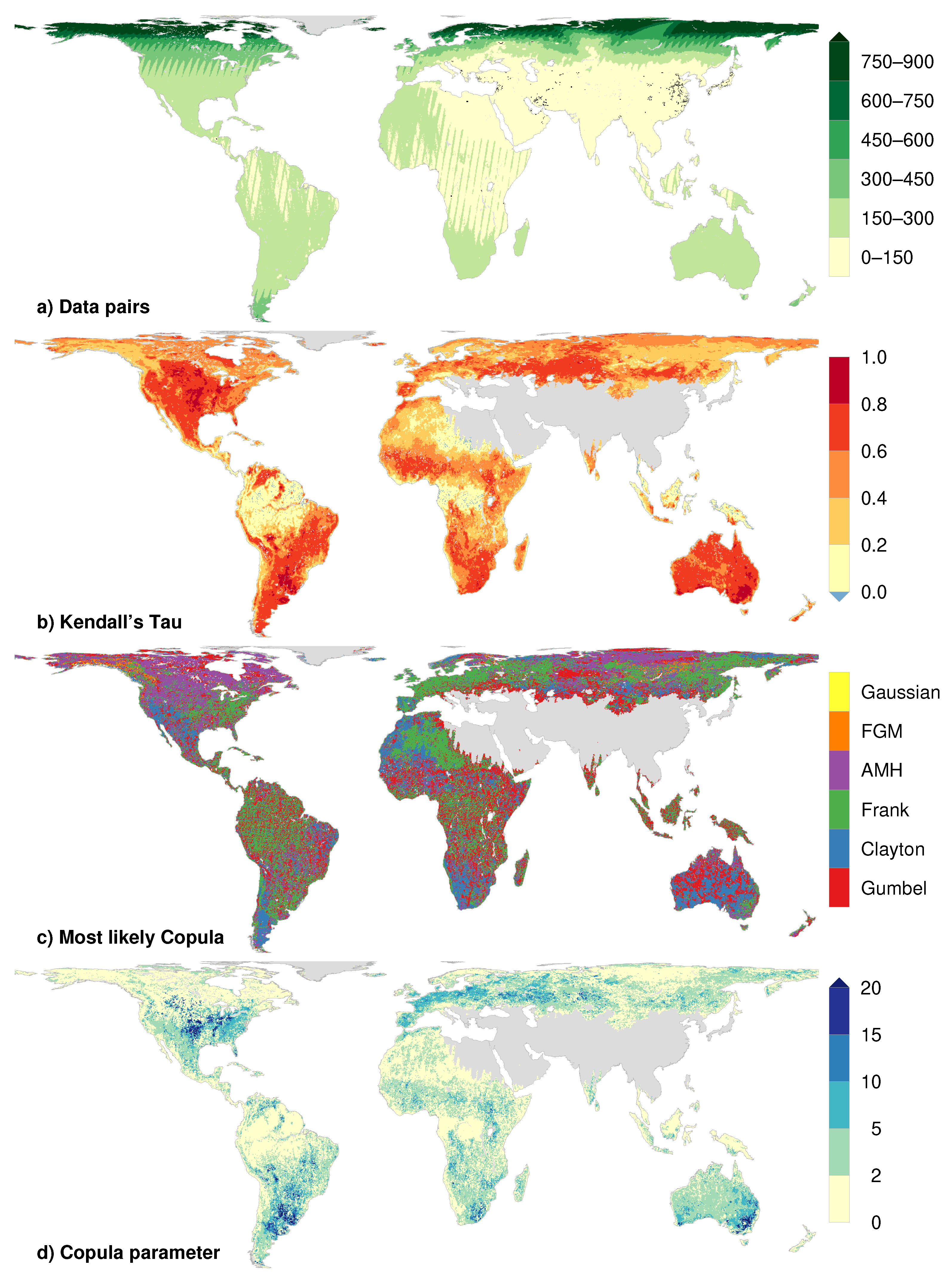
• Identification a suitable copula model $C\left(u,v\right)$ for modeling the bivariate dependency structure using the Bayesian copula selection from Huard et al. [79] (Section 3.3);
• Computation of the corresponding copula parameter $\theta$ using a Canonical Maximum Likelihood Estimate (CMLE) (Section 3.4);
• Conditioning of the copula CDF on SMAP_E Tb and drawing conditional random samples (Section 3.5);
• Inverse transformation of the random samples to the data space (Section 3.6);
• Computation of the full Tb-signal by adding back the mean annual cycle from SMAP_E to the transformed conditional random samples.

3.1. Step 1: Transformation to Anomalies

Hydrometeorological (here: soil moisture) or remote sensing (here: brightness temperatures) variables often underlie certain periodic effects like annual or daily cycles. These effects create an artificial dependency between variables by repeating the same periodic patterns, which superimposes the real statistical relationship. There are various methods to remove these periodical effects. As an example, Laux et al. [66] used an ARMA-GARCH approach for removing a large part of the autocorrelation in precipitation time-series. However, while such complex time-series models are justified from a statistical point of view, they can be difficult to interpret, as the residuals have only little physical meaning.

In this study, we therefore compute the mean annual cycle (i.e., an average for January, February, etc.) from SMOS and SMAP_E Tbs between April 2015 and March 2018, which is then removed from all datasets. We are well aware that the mean annual cycle from only three years of data might not be representative of the climatological behavior of Tbs. However, we are only interested in the removal of large parts of the periodic effects in the Tb time series, and we assume that monthly averages from three years of data are sufficient for this exemplary purpose.

3.2. Step 2: Estimation of the Marginals

The second step of the approach is the estimation of the marginals and the transformation of Tb anomalies to the unit interval or rank space (normalization), i.e.,

$$\begin{array}{cc}\hfill r_i& =F_X\left(x_i\right)\mathrm{with}{r}_i\in \left[0,1\right]\hfill \end{array}$$

(4)

$$\begin{array}{cc}\hfill s_i& =F_Y\left(y_i\right)\mathrm{with}{s}_i\in \left[0,1\right]\hfill \end{array}$$

(5)

where $x_i$ and $y_i$ are the SMOS- and SMAP_E-derived brightness temperature anomalies, $F_X$ and $F_Y$ the marginal distributions (CDFs) of SMOS and SMAP_E Tbs and $r_i$ and $s_i$ the CDF-transformed Tbs in a single 9 km pixel, respectively. It should be noted that we generally differentiate between the transformed Tb values r and s and the percentiles u and v, which can be computed by discretizing the unit interval into equally-sized bins and counting the number of r or s values until a particular bin or by simple interpolation.

There are multiple options for estimating these marginals, including both parametric, e.g., [63,67], and non-parametric, e.g., [61], methods. Similar to Laux et al. [66], we use a semi-parametric approach, where the interior of the distribution is estimated using a Gaussian kernel function. In order to compensate for the small number of samples in the tails, the upper and lower 10% of the CDF are approximated through a Generalized Pareto Distribution (GPD):

$$\begin{array}{cc}\hfill f\left(x\right)& =\frac{1}{\sigma }{\left(1+k\left(\frac{x-\theta }{\sigma }\right)\right)}^{-1-\frac{1}{k}}\hfill \end{array}$$

(6)

with the scale parameter $\sigma$, the shape parameter k and the location parameter $\theta$.

Several experiments have shown that this method usually results in higher copula parameters (Section 3.4) compared to, e.g., purely non-parametric estimates like the empirical CDF. This is due to the fact that the tails of the distributions are approximated with the same parametric model and therefore share similar characteristics. As the magnitude of the copula parameter is sensitive to these tails, this similarity leads to usually larger copula parameters and therefore to a higher dependency. It is noted that there might be cases where other fully-parametric distributions are slightly better suited. However, we assume that the kernel density estimate is more universal and flexible and thus more suitable for global-scale applications where an inspection and evaluation of each pixel’s distribution would be too computationally expensive.

3.3. Step 3: Identification of a Suitable Copula

There are multiple options for finding a copula that describes the dependency between SMOS- and SMAP-derived Tb. Many studies use the empirical copula [80]:

$$\begin{array}{cc}\hfill C_n\left(u,v\right)& =\frac{1}{n}\sum _{i=1}^n\mathbf{1}\left(\frac{r_i}{n}\le u,\frac{s_i}{n}\le v\right)\hfill \end{array}$$

(7)

where r and s are the CDF-transformed Tbs using the previously derived semi-parametric distributions (see Section 3.2). $\mathbf{1}\left(·\right)$ is the indicator function, which takes a value of 1 if the conditions in its argument are satisfied, u and v are the percentiles of SMOS- and SMAP_E-derived Tbs, and n is the number of samples. In analogy to the empirical CDF, this non-parametric, empirical copula-CDF can be computed by discretizing the unit interval into equally-sized bins and counting the number of r and s values up to a particular u and v bin. After estimating the copula parameter (Section 3.4) for a pre-defined set of theoretical copulas, the empirical copula is compared against the theoretical models using, e.g., the Cramér–von Mises statistic [81] or deterministic error measures like the RMSE [82]. In this study, we use a set of six different copula models, namely the Clayton, Frank, Gumbel, Farlie–Gumbel–Morgenstern (FGM), Ali–Mikhail–Haq (AMH) and Gaussian copulas (see Appendix A). Using different copula models allows for a better representation of specific dependency structures between two random variables (here: the SMOS- and SMAP_E-derived Tbs). In general, the main difference is the description of the tail dependencies, i.e., the dependencies of the very high and low values. While the Clayton and Gumbel copulas are suitable for strong left and right tail dependence, respectively, the symmetric Frank copula describes stronger dependencies in the center of the distribution. The FGM-copula can be used if the dependency is relatively low, while the Gaussian copula is highly flexible, as it can describe both positive and negative dependencies [69]. A comprehensive list of different copula models, as well as their characteristics can be found in Nelsen [78].

A suitable copula is then identified, e.g., by parametric bootstrapping [83]. However, especially the bootstrapping requires large computational effort, as it needs a reasonably large number of resamples. Such methods are hence only of limited use for global-scale applications due to the large number of pixels. We therefore use a Bayesian approach, which has been proposed by Huard et al. [79]. The main difference is that we do not have to compute a copula-parameter in advance, but we first identify the most likely copula from which the random samples (i.e., the CDF-transformed Tbs) are drawn and then estimate the corresponding parameter. This is achieved by treating the copula parameter as nuisance variables and parameterizing the copula density in terms of the rank correlation coefficient, i.e., Kendall’s $\tau$. The distribution of $\tau$ is then used as prior probability distribution within a Bayesian framework. For every grid cell, we compute the likelihood of the different copula models, which are listed in

Table A1. Copulas tested in this study including the definition and the ranges of the copula parameter $\theta$ and the corresponding rank correlation coefficient $\tau$.

Copula	${\mathit{C}}_{\mathit{\theta }}\left(\mathit{u},\mathit{v}\right)$	$\mathit{\theta }$	$\mathit{\tau }$
Clayton	${\left(u^{-\theta }+v^{-\theta }-1\right)}^{-\frac{1}{\theta }}$	$\left(0,\infty \right)$	$\left[0,1\right]$
Frank	$-\frac{1}{\theta }ln\left(1+\frac{\left(e^{-\theta u}-1\right)\left(e^{-\theta v}-1\right)}{e^{-\theta }-1}\right)$	$\left(-\infty ,\infty \right)\backslash 0$	$\left[-1,1\right]\backslash 0$
Gumbel	$exp\left(-{\left({\left(-lnu\right)}^{\theta }+{\left(-lnv\right)}^{\theta }\right)}^{\frac{1}{\theta }}\right)$	$\left[1,\infty \right)\backslash 0$	$\left[0,1\right]$
FGM	$uv+\theta uv\left(1-u\right)\left(1-v\right)$	$\left[-1,1\right]$	$\left[-\frac{2}{9},\frac{2}{9}\right]$
AMH	$\frac{{\displaystyle uv}}{{\displaystyle 1-\theta \left(1-u\right)\left(1-v\right)}}$	$\left[-1,1\right]$	$\left[-0.181726,\frac{1}{3}\right]$
Gaussian	${\displaystyle \frac{1}{{\displaystyle 2\pi \sqrt{1-{\theta }^2}}}{\int }_{-\infty }^{{\varphi }^{-1}\left(u\right)}{\int }_{-\infty }^{{\varphi }^{-1}\left(v\right)}exp\left(\frac{2\theta s\omega -s^2-{\omega }^2}{{\displaystyle 2\left(1-{\theta }^2\right)}}\right)}$	$\left[-1,1\right]$	$\left[-1,1\right]$

. The model with the largest probability (i.e., p-value) is then selected for the subsequent computations. This method has been used successfully in multiple hydrological applications, e.g., [63,69,84].

3.4. Step 4: Computation of the Copula Parameter

After a suitable copula has been identified, the corresponding copula parameter $\theta$ is computed. A widely-used method is the relationship between the copula parameter and the rank correlation coefficient, i.e., Kendall’s $\tau$:

$$\begin{array}{cc}\hfill \tau & =4{\int }_0^1{\int }_0^1{C}_{\theta }\left(u,v\right)d{C}_{\theta }\left(u,v\right)-1\hfill \end{array}$$

(8)

where $C_{\theta }$ denotes a specific copula with the parameter $\theta$. For bivariate Archimedean copulas, which are explicitly defined through:

$$\begin{array}{cc}\hfill C_{{\varphi }_{\theta }}\left(u,v\right)& ={\varphi }_{\theta }\left({\varphi }_{\theta }^{-1}\left(u\right)+{\varphi }_{\theta }^{-1}\left(v\right)\right)\hfill \end{array}$$

(9)

with the generator $\varphi$, Genest and MacKay [85] showed that:

$$\begin{array}{cc}\hfill \tau & =1+4{\int }_0^1\frac{{\varphi }_{\theta }\left(t\right)}{{\varphi }_{\theta }^{\prime }\left(t\right)}dt,\hfill \end{array}$$

(10)

where ${\varphi }_{\theta }^{\prime }\left(t\right)$ is the first derivative with respect to the parameter t. For some copulas, there is a closed expression for this relationship, i.e., we can directly compute the copula parameter from Kendall’s $\tau$. In turn, this link allows one to interpret the copula parameter as a measure for the strength of dependence: higher copula parameters reveal a stronger dependence [66]. It should be noted, though, that the magnitude of the copula parameter depends significantly on the chosen copula (see Table A1). Thus, different copula parameters must always be compared by considering the respective copula family.

Kim et al. [86] analyzed the performance of several parameter estimation approaches and concluded that if the marginal distributions are not known, the Canonical Maximum Likelihood Estimation (CMLE; Genest et al. [87]) performs best. We therefore decided to use CMLE, as it also provides a faster and more efficient way (compared to the inversion of $\tau$) to estimate $\theta$.

3.5. Step 5: Conditional Sampling

After estimating the copula parameter, the so-called conditional copula is calculated:

$$\begin{array}{cc}\hfill P\left(V\le v|U=r\right)& ={\left.\frac{\partial C\left(u,v\right)}{\partial u}\right|}_{u=r}\hfill \end{array}$$

(11)

In the bivariate case, this conditional copula is simply the uniform CDF for the variable V under the constraint that U takes the value r. Here, the copulas in every single 9 km grid cell are conditioned on the SMOS Tbs, which means that we take a single CDF-transformed SMOS-Tb value $r_i$ and evaluate the partial derivative of the copula $\frac{\partial C\left(u,v\right)}{\partial u}$ at that particular location. This allows for the estimation of a conditional SMAP_E-like CDF for each daily SMOS value within every 9 km grid cell at that particular location. These CDFs are now used to generate a sufficiently large number of conditional random samples $v_{i,u=r_i}$ for every SMOS Tb $r_i$ during the full study period April 2010–March 2018. Here, we decided to use 500 samples as a compromise between a statistically-sufficient sample size and computational costs.

3.6. Step 6: Inverse Transform of Random Samples

From these 500 values, we compute the mean ${\overline{v}}_{i,u=r_i}$ and, as a measure for the robustness of the estimated Tbs, the standard deviation, which are then transformed back to the data-space using the inverse probability integral transformation:

$$\begin{array}{cc}\hfill {\overline{v}}_{i,u=r_i}=F_Y\left(y_{i,u=r_i}\right)& \iff y_{i,u=r_i}=F_Y^{-1}\left({\overline{v}}_{i,u=r_i}\right).\hfill \end{array}$$

(12)

It should be noted that we can also use the median instead of the mean and the median absolute deviation instead of the standard deviation for the subsequent computations. However, we think that the mean and standard deviation are more descriptive and easier to interpret in this context. For each SMOS Tb value in every grid cell and point in time, we therefore obtain an SMAP_E-like Tb and a corresponding uncertainty estimate through its standard deviation.

In the end, the mean annual cycle removed in Step 1 is added back to the data to obtain the final Copula-combined SMOS-SMAP_E (CoSMOP) product. Here, we add back the mean annual cycle of the SMAP_E product, which has a spatial posting of 9 km. However, it is also possible to add back the mean annual cycle of SMOS in a similar way, but this is available just at the coarse resolution of SMOS, so that it defeats the purpose of resolution enhancement.

3.7. Validation Procedure

While the CoSMOP-Tb product is available at the global scale, we perform our validation at the Tb level over the Contiguous United States (CONUS) only. As only a few long-term time series of Tb records are available worldwide, a comparison towards Tb forward simulations using time series from the USDA Natural Resources Conservation Service Soil Climate Analysis Network (SCAN) [88] is performed. As SCAN includes around 200 stations, this validation strategy allows for the long-term comparison of satellite- and station-based brightness temperatures over almost the whole CONUS domain, in contrast to the evaluation against directly observed Tbs from, e.g., field campaigns, which are available for only limited points in time and space.

Forward calculations of Tb are performed by the L-Band Microwave Emission of the Biosphere Model (L-MEB) [89]. L-MEB is a so-called τ-ω model, where the radiative transfer in the vegetation layer is described through its optical depth τ and single scattering albedo ω. It shares the same procedures as the SMOS L2 soil moisture processor. The Mironov dielectric mixing model has been implemented to convert the measured soil moisture into a dielectric constant [90].

For the SCAN sites where top soil moisture (−5 cm), top soil temperature (−5 cm), soil temperature in depth (−50 cm), as well as air temperature in 2 m height are available in hourly resolution as forcing data for L-MEB, Tb time series in H- and V-pol have been generated [91]. For consistency with SMAP, the SMAP auxiliary soil parameters sand fraction, silt fraction and soil bulk density are utilized [92], as well as the respective vegetation opacity map from the SMAP Enhanced L3 Soil Moisture product [93].

From the whole network, which consists of more than 200 stations, we removed the stations that are located outside the CONUS-region and that do not provide the information necessary for the L-MEB approach. We further defined two validation periods in order to analyze the performance of CoSMOP during the pre-SMAP-period, but also against SMAP_E-derived Tbs:

• Single mission period from April 2010 to March 2015: Comparison of SMOS and CoSMOP with L-MEB
• Dual mission period from April 2015 to March 2018: Comparison of SMOS, SMAP_E and CoSMOP with L-MEB

From the remaining list of stations, we therefore removed all sites that have less than one year of observations in the first or second period, which results in 149 stations (blue dots in Figure 1). We also defined a set of 53 stations with almost continuous records (i.e., at least 80% during Period 1 and 2, respectively; see the red dots in Figure 1). The comparison of SMOS, SMAP_E and CoSMOP against the Tb-data generated by L-MEB is carried out over all 149 stations for analyzing the robustness and performance over as many locations as possible, but also for the 53 stations for analyzing the long-term performance.

All station-based brightness temperatures are corrected for outliers, as some stations occasionally show extreme Tbs. The values that deviate more than three-times the standard deviation from the mean (for each station) are removed.

Similar to [60], we do not only consider the grid cell in which the station is located, but also the neighboring pixels, as the closest pixel might not be the most representative. Here, we assume a search radius of 9 km, which results, depending on the relative position of the station with respect to the 9 km EASE 2.0 grid, in an average over two to four pixels.

There might be, however, a general mismatch between the magnitude of the L-MEB and the Tb observations. This can be seen when, e.g., the CDFs from the satellite and the simulated SCAN Tbs are compared (not shown).

As the station data are not considered in the data fusion, it is not expected that the approach is able to correct for that inconsistency. Therefore, we first remove the average Tb from April 2015 to March 2018 from all datasets. The comparison with the L-MEB Tbs is therefore carried out at the anomaly level.

These anomalies from SMAP_E, SMOS and CoSMOP are then compared against the station-based anomalies in terms of the RMSE:

$$\begin{array}{cc}\hfill RMSE& =\sqrt{\frac{1}{N}\sum _{n=1}^N{\left(T{b}_{n,sat}-T{b}_{n,lmeb}\right)}^2}\hfill \end{array}$$

(13)

and the Nash-Sutcliffe-Efficiency (NSE)

$$\begin{array}{cc}\hfill NSE& =1-\frac{{\displaystyle \sum _{n=1}^N{\left(T{b}_{n,sat}-T{b}_{n,lmeb}\right)}^2}}{{\displaystyle \sum _{n=1}^N{\left(T{b}_{n,lmeb}-{\overline{Tb}}_{n,lmeb}\right)}^2}}.\hfill \end{array}$$

(14)

The $T{b}_{n,sat}$ are the spaceborne recorded Tbs from SMOS, SMAP_E and CoSMOP at the locations of the stations, $T{b}_{n,lmeb}$ the forward-modeled (L-MEB) Tbs from the soil moisture observation stations and N the number of simultaneous retrievals. The RMSE is used here as an absolute error metric, while the NSE, according to Lorenz et al. [94], is the normalized mean absolute error and more sensible for the overall performance of the estimates.

4. Results and Discussion

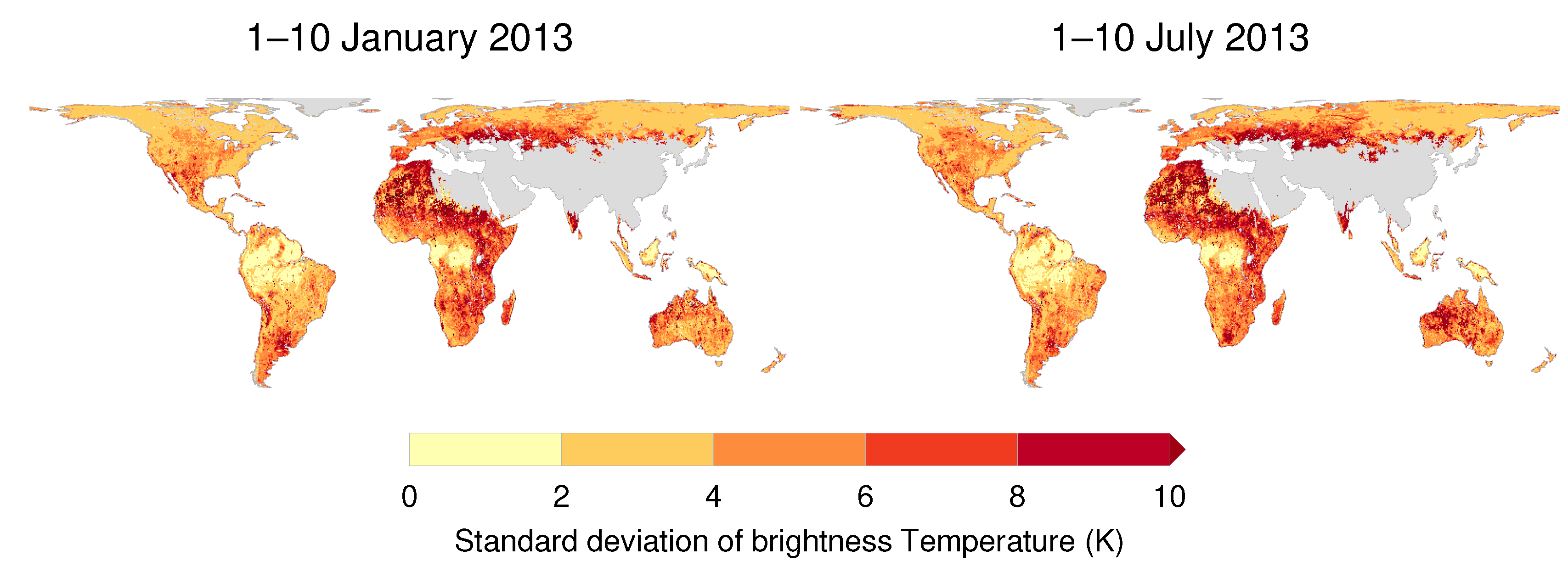
4.1. Basic Properties of the Merged Data

One critical issue about any statistical merging technique is the number of (simultaneous) samples for estimating the joint distribution. Here, we are using three years of data from SMOS and SMAP_E, which roughly provide one retrieval for each pixel every three days. We further select a time window of a maximum of 6 h between the retrieval of SMAP and SMOS. Due to the opposing orbits of SMAP and SMOS, however, the number of data pairs depends on geographic latitude. Figure 2a therefore shows the number of pairs that have been used for fusing data from SMOS and SMAP. Especially over the higher northern and southern latitudes, there are more than 900 pairs for estimating the copula and the corresponding parameters. In the mid-latitudes, there are still more than 250 pairs, while this number decreases to around 150 pairs over the equatorial regions. The SMOS data over large parts of Northern Africa and the whole of Asia, however, suffer from high Radio Frequency Interference (RFI) for the SMOS product [73]. These areas usually show less than 100 simultaneous retrievals, which does not allow the reliable estimation of the dependency structure within the copula-based approach so far. We therefore removed these regions from this study.

Due to the relationship between Kendall’s rank correlation and the copula (higher rank correlations imply, depending on the fitted copula model, higher copula parameters; see Section 3.4), an analysis of the correlation in each pixel already indicates the magnitude of the similarities between SMAP_E and SMOS. Therefore, Figure 2b shows Kendall’s $\tau$, which is derived from brightness temperature anomalies during the calibration period April 2015–March 2018. The rank correlation between SMOS and SMAP_E Tbs depends significantly on the land cover and vegetation types. Especially over shrublands, grasslands or similar vegetation classes, rank correlations above 0.8 can be observed. Over densely-vegetated areas, like the tropical rain forest, however, the rank correlations drop to values around zero. It should be noted that the rank correlation coefficient is based on the Tb anomalies, where the annual cycle has been removed. Low rank correlations over the tropics are thus also an indicator for a highly periodic and dominant annual cycle, which does not change significantly from year to year. The remaining anomalies from SMOS and SMAP_E have nothing in common, which leads to both low rank correlation values and low copula parameters.

The relatively small number of data pairs, together with the low correlations, also affect the robustness of the derived copulas and their parameters for the equatorial regions. This can be seen in Figure 2c, which shows the most likely copula models (i.e., the models with the highest p-values) for every grid cell. Especially over regions with low rank correlation coefficients, the identified copula models show highly scattered patterns and the derived copula parameters (Figure 2d are relatively low with values close to zero.

From around ${25}^{\circ }$ north and south, the patterns are getting more stable as more than 200 pairs can be used and the vegetation is less dense. For mid-latitude regions over large parts of the Eurasian continent and the eastern part of North America, the Frank copula is the most appropriate model; the AMH-model is identified especially over the higher latitudes over the North American continent and Siberia. However, especially the Gumbel-copula does not appear over larger areas, but rather scattered across the globe. Interestingly, the Gaussian and FGM-copula appear only in a very limited number of pixels.

The spatial dependency of the copula types is not yet fully understood. However, as there are significantly larger continuous copula-patterns over the higher latitudes, we assume that the scattered results around the Equator are mainly due to the relatively low number of samples. This leads to less robust estimates of the tails of the marginal distributions from SMAP_E and SMOS. In terms of copulas, however, the regions at the edges of the marginals are extremely important as one of the biggest differences of the copula models is the description of tail dependencies. Similar to, e.g., the correlation coefficient from a very small number of samples, the fitted copula model can change due to minor differences in the brightness temperatures at adjacent locations. However, as both SMOS and SMAP are still in service, it is planned to extend the calibration period in the future to increase the number of pairs and therefore obtain more robust results, especially over the low-latitude regions.

By definition, the patterns of Kendall’s $\tau$ (Figure 2b) and the copula parameter $\theta$ (Figure 2d) are very similar. The high-correlation regions across North and South America, as well as Eurasia also show relatively high copula parameters. Again, low parameters can be observed especially over the tropical rainforest, but also over the high latitudes. Over these regions, the AMH-copula is usually identified as the best model with parameters around $0.7$. As the AMH-copula parameter is bound between $-1$ and 1, such values still indicate a high relationship between SMAP_E and SMOS and correspond to rank correlation coefficients of around $0.5$.

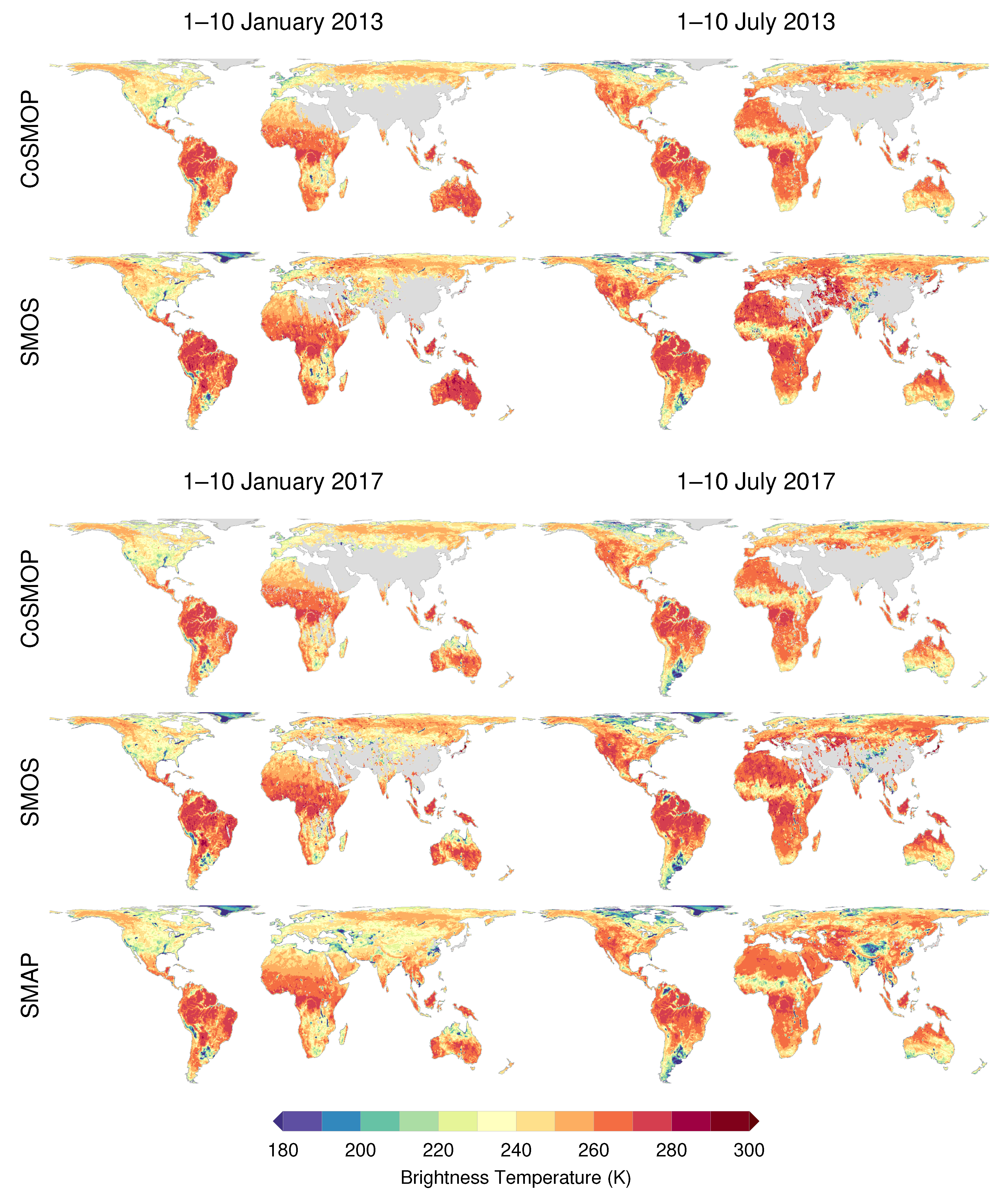
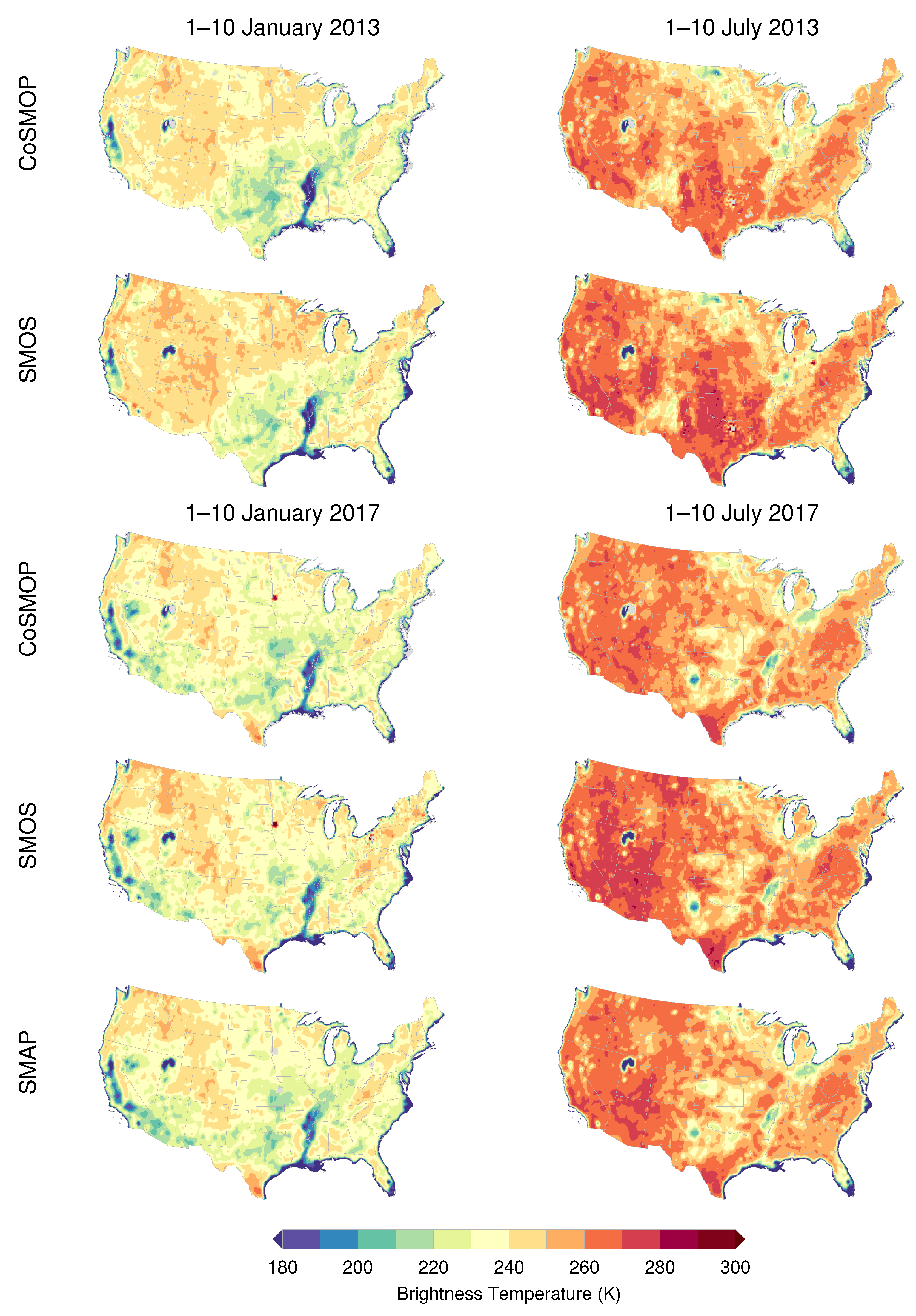
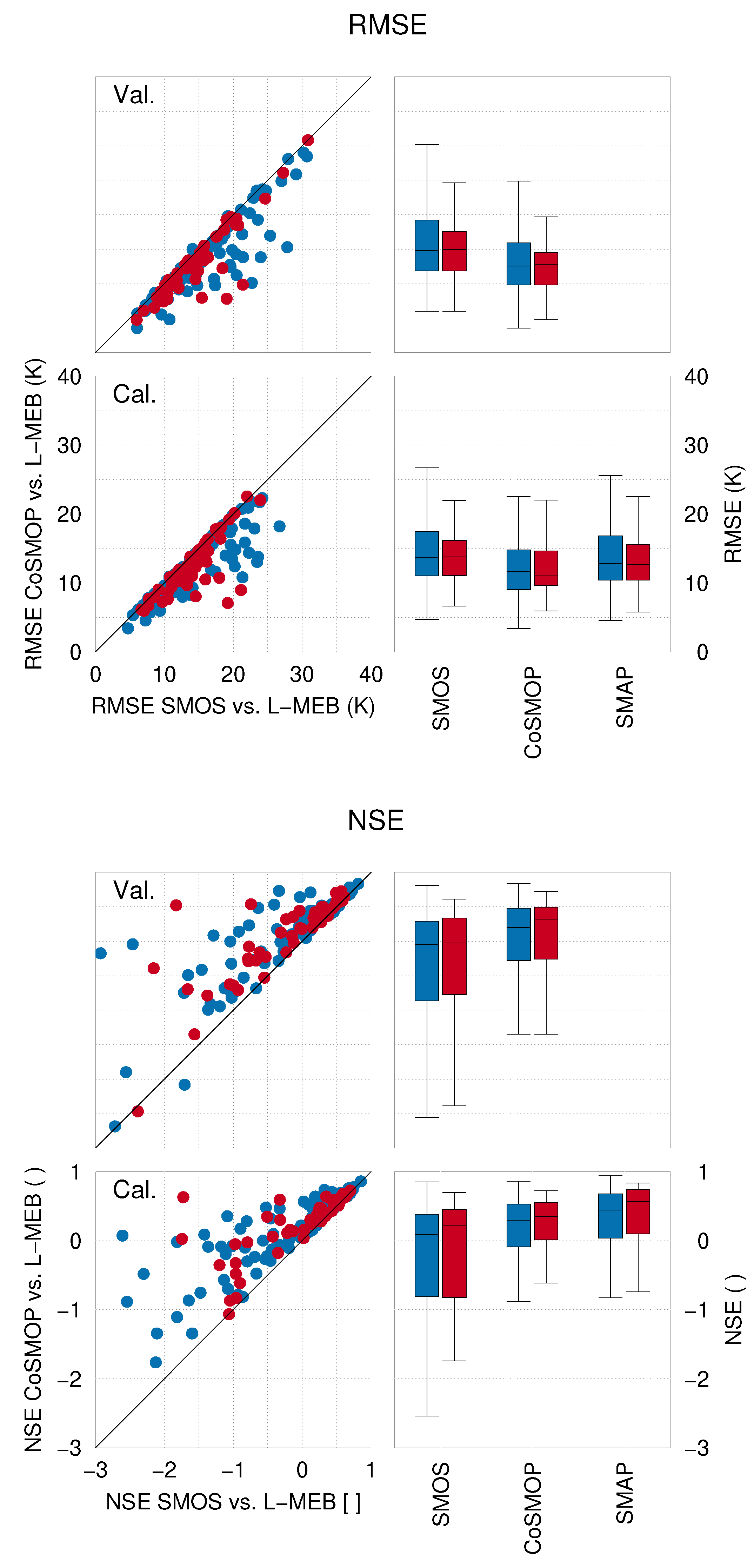
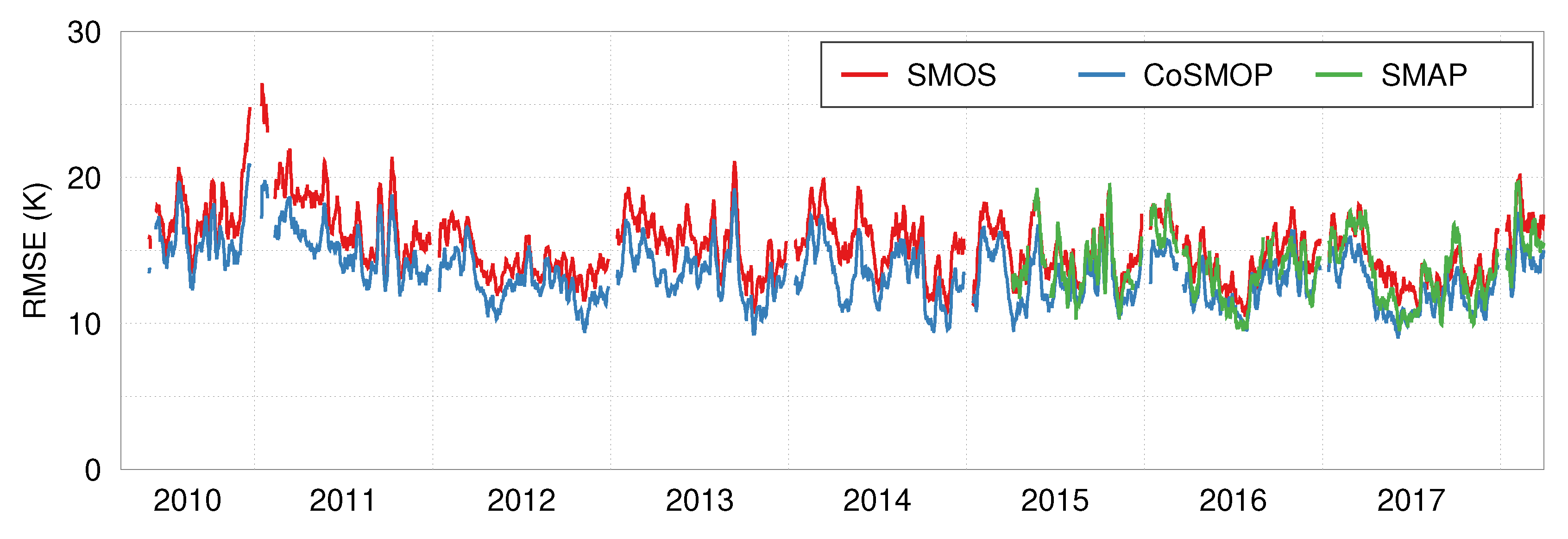
4.2. Comparison of SMOS, SMAP_E and CoSMOP

The final daily CoSMOP product is provided at 9 km resolution for the period April 2010–March 2018. Figure 3 shows 10-day averaged Tbs from CoSMOP, SMAP_E and SMOS during the period from 1 to 10 January 2013 and 2017 (Northern Hemispheric (NH) winter, left column) and from 1 to 10 July 2013 and 2017 (Southern Hemispheric (SH) winter, right column). At the global scale, there are no significant differences between the three products. The derived fields agree very well in terms of their patterns and magnitudes. In some regions, the Tbs of CoSMOP tend to slightly lower values compared to the other two products. This can be seen especially over North America and the low-temperature regions in the southeastern regions and central west coast of South America. The same holds true for the SH-winter fields.

On the global maps of Figure 3, the improvement in scale between 9 km SMAP_E and CoSMOP compared to the coarser 25 km SMOS fields is not visible. For comparison, Figure 4 shows Tbs over the CONUS domain only. During January, the patterns and magnitudes from SMAP_E and SMOS are again very similar with low values of 180 K and less especially west of the Sierra Nevada, the region around the Salt Lake and along the Mississippi River. In July, high values can be observed across the whole USA, while the SMOS records are slightly higher than the SMAP_E Tbs.

Besides the slightly lower values, the 9 km fields from CoSMOP and SMAP_E show slightly smoother patterns than the original SMOS data. However, SMAP was developed to provide a spatial resolution of 36 km, and the used 9 km SMAP_E product is a result of an interpolation. Although the Backus–Gilbert interpolation is known to be a robust approach, the interpolative character is still visible in SMAP_E data and therefore also in the CoSMOP product with a similar level of detail. However, even the smoother patterns can cause large differences if, e.g., derived soil moisture estimates are used for hydrological modeling.

When comparing the CoSMOP fields during both the validation and calibration periods, it becomes evident that the data fusion successfully improves the spatial resolution and magnitudes of SMOS-derived Tbs also during the pre-SMAP period, which, in the end, provides a consistent time-series of CoSMOP Tbs from 2010 to the present.

In order to analyze the uncertainty of the CoSMOP brightness temperatures, Figure 5 shows the 10-day averaged standard deviations (i.e., the square root of the average variances) of the CoSMOP-Tbs for two different periods in the NH-winter and SH-winter. These standard deviations describe the spread of the conditional random samples and by that the width of the conditional copula PDFs (Section 3.5). Usually, large copula parameters indicate a high level of dependency, which finally result in narrow conditional distributions and small standard deviations. Figure 5 strongly resembles the correlation patterns in Figure 2 with low values, especially over the tropical rainforests. The largest standard deviations can be observed over the vast African deserts. Here, the low correlation, together with low Frank-copula parameters, clearly indicate a high level of uncertainty in the CoSMOP product. Over most other regions including the CONUS-domain, the standard deviation is between 2 K and 6 K. Based on the natural magnitudes and dynamics of Tbs, such values can be expected. Nevertheless, it needs to be further investigated if and how the spread in the conditional random samples can be decreased in order to improve the sharpness of the CoSMOP-Tbs.

In contrast to the clear NH- and SH-winter signals in Figure 3, the standard deviations show only small temporal variations. There are small deviations, e.g., over South Africa or Australia, but most large-scale patterns remain similar. This also indicates that for most regions, the uncertainty does not depend too much on the chosen period and remains rather constant.

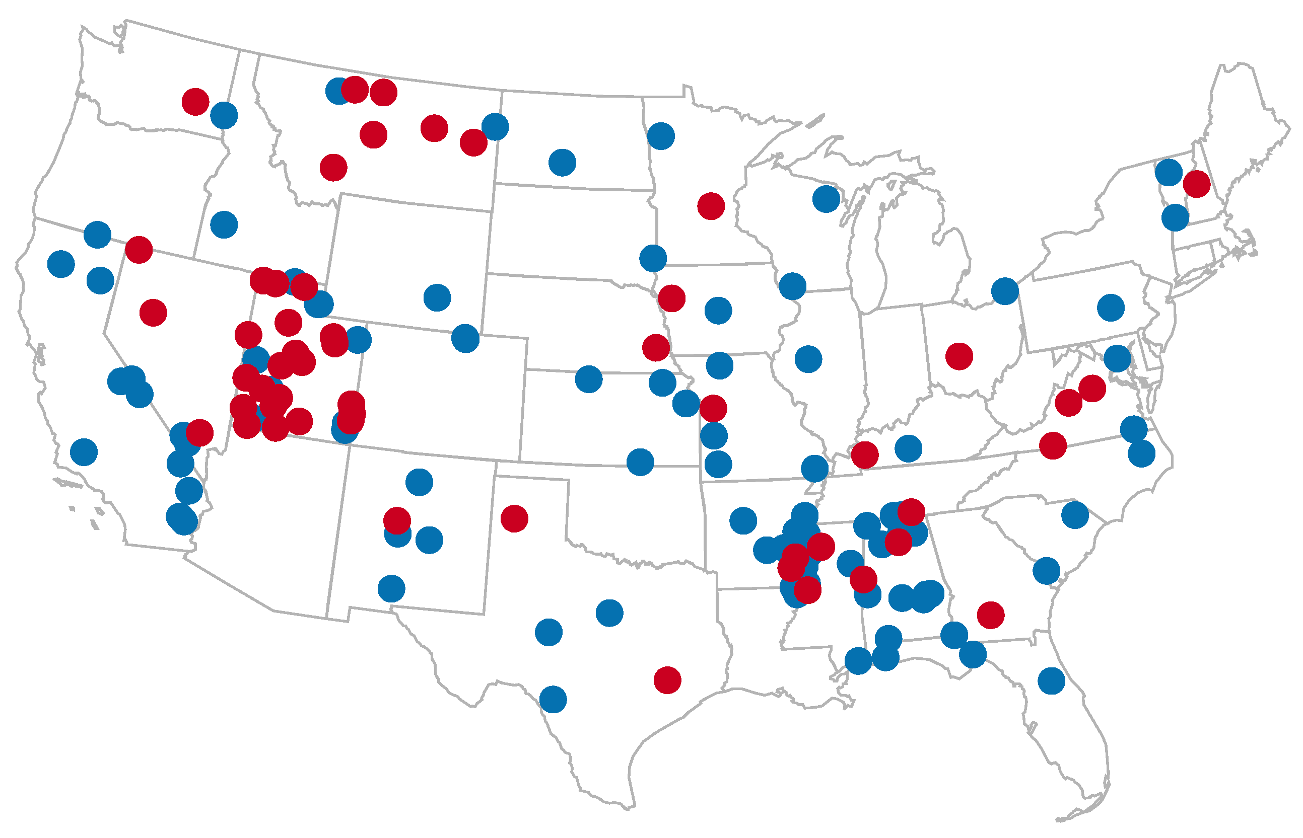
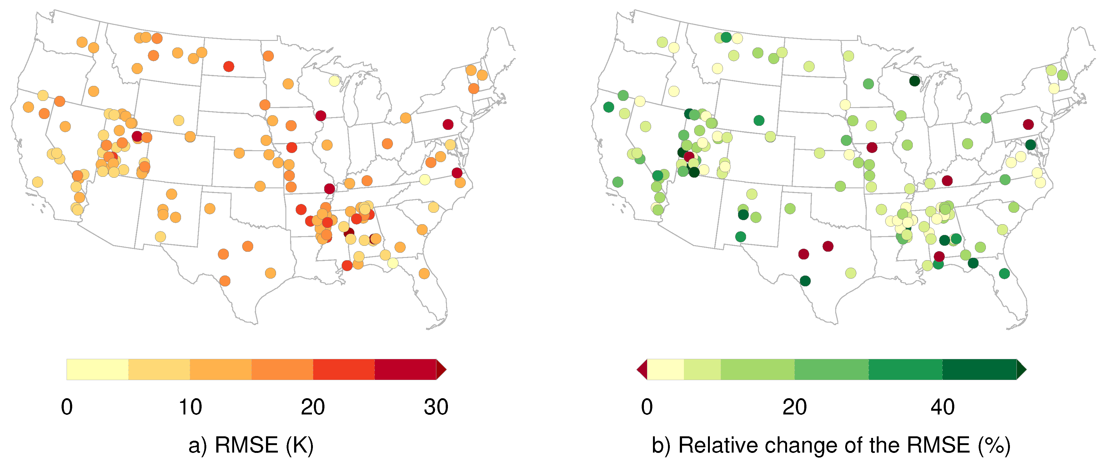
4.3. Comparison against Brightness Temperatures Simulated over SCAN Stations

Figure 6 shows the RMSE between CoSMOP and L-MEB forward simulated Tb over SCAN sites and the improvement compared to the original SMOS data between the period April 2010 and March 2015. The average RMSE and median NSE (We use the median here due to the usually highly skewed distribution of NSE-values. The mean would give a negatively-distorted view due to several negative values.) during the two validation periods over all stations and the pre-defined subset are depicted in

Table 1. Average performance (median NSE and mean RMSE) between SMOS-, SMAP_E- and CoSMOP-derived daily brightness Temperatures (Tbs) as compared to L-Band Microwave Emission of the Biosphere Model (L-MEB) simulations over 149 SCAN sites for a single-mission period (top) and a dual-mission period (bottom); the values in brackets are the metrics over 53 stations with almost continuous records.

Period	Dataset	NSE	RMSE
Single-mission period	SMOS	−0.05 (−0.03)	15.85 (15.14)
	CoSMOP	0.20 (0.32)	13.69 (13.20)
	SMOS	0.09 (0.21)	14.26 (13.97)
Dual-mission period	CoSMOP	0.30 (0.35)	12.21 (12.18)
	SMAP_E	0.44 (0.56)	13.48 (13.05)

. Figure 7 shows scatter and boxplots of the RMSE and NSE between SMOS, SMAP_E, CoSMOP and L-MEB, where the colors depict the ensemble of all stations (blue) and the pre-defined subset with continuous records (red).

Over 142 out of the 149 stations and within both validation periods, CoSMOP shows significantly better results compared to SMOS (see Figure 6 and Table 1). Overall, the mean RMSE from SMOS during the single mission period over all and the selected stations can be reduced from 15.85 K to 13.69 K and from 15.14 K to 13.20 K, respectively. Over some stations, the RMSE from CoSMOP is even more than 40% lower compared to SMOS. The same holds true for the median NSE, which can be improved from around 0–0.2 and 0.32 for all and the selected stations, respectively. Besides the improvement of the average performance, the spread of the RMSE and NSE values from CoSMOP (depicted by the length of the whiskers in Figure 7) is much lower compared to SMOS. Therefore, it can be assumed that the Tbs from CoSMOP have much more homogeneous magnitudes compared to SMOS and thus provide more consistent estimates.

The metrics in Table 1 indicate that the performance during the dual mission period is slightly better compared to the pre-SMAP-period. The RMSE from SMOS decreases by around 1.5 K from 15.85 K to 14.26 K and from 15.14 K to 13.97 K for all and the selected stations, respectively. The same holds true for the NSE, which increases from around 0–0.09 and 0.21. The level of improvement from SMOS to CoSMOP, however, is very similar during both periods. The RMSE (NSE) is generally decreased (increased) by around 2 K (0.2). This is confirmed by Figure 8, which shows the 10-day averaged RMSE from SMOS, SMAP_E and CoSMOP with respect to L-MEB over the 53 selected stations during the period 2010–2018. In general, the temporal dynamics from all three satellite-based products are comparable. However, there is a significantly lower error level in CoSMOP compared to SMOS. Especially during 2010/2011, there are distinct peaks in the SMOS errors. Even if these peaks are still visible in CoSMOP, the magnitudes are much lower. The errors from CoSMOP and SMAP_E (from April 2015 onward) are comparable, even though CoSMOP shows a slight improvement. Overall, there is no obvious seasonality of the errors.

According to Figure 6, there is no clear pattern or local dependency of the improved performance. This is also reflected by the similar level of improvement between SMOS and CoSMOP from all stations and the pre-defined subset (Table 1). However, an analysis of the soil types of all the station data might give more insight into connections between the local (site) characteristics and the performance of CoSMOP. This will be evaluated in future studies.

The level of further improvement does not significantly depend on the identified copula.

Table 2. Average RMSE (K) for each copula over all SCAN stations in the CONUS region. The number in the brackets shows the number of stations where a specific copula has been identified. The two top rows show the values for the validation (i.e., pre-SMAP) period, while the three bottom rows correspond to the calibration period.

Period	Dataset	Gumbel (38)	Clayton (33)	Frank (46)	AMH (32)
Single-mission period	SMOS	17.32	13.84	16.53	15.20
	CoSMOP	14.39	11.88	14.61	13.42
Dual-mission period	SMOS	15.66	12.87	14.85	13.22
	CoSMOP	12.65	11.10	13.18	11.47
	SMAP_E	13.90	12.70	14.28	12.66

shows the average root mean squared error over all stations in the CONUS region with the same copulas. For the reduced station number with 80% data availability, the metrics may not be statistically sound. Nevertheless, at least for the locations where the Gumbel copula is identified, the RMSE of SMOS is higher compared to the other locations, and CoSMOP shows an improvement of around 3 K during both validation periods.

One of the main reasons for this generally improved performance is the reduction of the variance in the CoSMOP Tbs due to the copula fitting, which is generally too high in the original SMOS records. The copula describes the signal dependency between SMOS and SMAP_E if we assume the noise in the two original products to be uncorrelated. Hence, the conditional random samples are based on the noise-free part of the Tbs from SMOS and SMAP_E, which leads to a lower noise level in the CoSMOP-Tbs. Another reason is the higher spatial resolution of 9 km. We assume a radius of 9 km around each pixel, from which we then average the satellite Tbs. Thus, the spatially higher resolved fields reflect the local characteristics more reasonably than the original 25 km pixels from SMOS. This higher spatial resolution together with more homogeneous patterns and consistent Tb-dynamics leads to more reliable and reasonable Tb estimates. Especially when the derived brightness temperatures are transformed to soil moisture, the more consistent CoSMOP product should provide superior performance compared to SMOS when, e.g., used as input for hydrological modeling approaches.

5. Conclusions

A copula-based approach for merging brightness temperatures from SMOS and SMAP enhanced is developed and analyzed for generating the high resolution (9 km), long-term (2010–2018), global copula-combined SMOS-SMAP_E product CoSMOP. In particular, the approach exploits the joint temporal dependency structure between the two satellite-based datasets for constructing an SMAP_E-like time-series even for pre-SMAP periods from SMOS. This statistical consistency incorporates both a better spatial resolution and a significantly lower noise level. The copula-based approach allows for high flexibility in terms of the underlying marginal distributions and the joint dependency structure and is therefore proposed for global-scale data fusion applications where statistical requirements (e.g., normal distribution of the samples) are often difficult to achieve.

A joint analysis of the rank correlation parameter Kendall’s $\tau$, the estimated copula model and the corresponding parameter $\theta$ shows that the reliability of the derived CoSMOP product depends significantly on (a) the latitude and (b) the vegetation density. In general, especially the mid- to high-latitudes allow an estimation of the mandatory parameters with 300–950 samples. Over these locations, large contiguous patterns of similar copula models, relatively high correlation coefficients and, depending on the identified copula, high copula parameters can be derived. Over low-latitudes and dense vegetation areas (e.g., tropical rain forest), the correlation between SMOS and SMAP_E is much lower, which also results in low copula parameters and highly scattered copula models.

As both SMOS and SMAP are still in operation, it is planned to continuously extend the CoSMOP time series. Hence, the number of simultaneous radiometer-based observations will be increased in the future, which also will improve the reliability of the CoSMOP brightness temperatures. At the moment, especially the CoSMOP-Tbs over mid- to high-latitudes are assumed to be robust estimates, as they are based on a reasonable number of samples.

This is confirmed by the comparison against simulated brightness temperatures over SCAN sites driven by in situ measurements within the L-MEB model. For analyzing both the spatial and temporal consistency of CoSMOP, the derived Tbs are compared against 149 stations across the whole CONUS-domain and 53 pre-defined stations with almost continuous records during the period 2010–2018. In general, the root mean squared error can be improved for 142 out of the 149 stations by 2 K, which corresponds to around 15%. The same holds true for the Nash–Sutcliffe efficiency, which is increased from around 0–0.2 and 0.3 for all and the pre-defined ensemble of stations, respectively. The improvements seem to be independent of the region and also the identified copula. Nevertheless, the locations where the Gumbel-copula is identified show slightly larger errors compared to other regions. Thus, it will be part of future studies to see if there is a relationship between the CoSMOP performance and the study area (e.g., due to specific climatic conditions) or the identified copula. It will be further investigated if the performance of CoSMOP can be increased, e.g., by incorporating more copula models or by merging, e.g., the data from both SMOS’ and SMAP’s ascending and descending nodes, which will significantly increase the number of samples at the expense of the temporal representativeness of the derived statistics. While this study focuses on the global scale and the introduction of the CoSMOP product in general, it will be part of future studies to evaluate the performance of our brightness temperatures against data from field campaigns like, e.g., the SMAP Validation Experiment 2012 (SMAPVEX12).

On basis of our merged CoSMOP brightness temperature time series, a number of higher level products can be generated. In addition to soil freeze-thaw indication, also a global soil moisture time series can be generated by subsequent application of the Single-Channel Algorithm (SCA) [95] as the SMAP Level 2 processor. The chance to use alternative soil moisture retrieval approaches, e.g., the Dual-Channel Algorithm (DCA), is still persistent. Subsequent CoSMOP studies will focus on such a transformation to, e.g., soil moisture and the performance gain compared to the original SMOS estimates. Our study is the first step towards long-term, high-resolution and consistent time-series of remote sensing-based brightness temperatures, which ultimately have the potential to improve our knowledge about many aspects of the global climate system, including the long-term evolution of global-scale soil moisture.

The CoSMOP brightness temperatures are freely available (after registration) at https://thredds.imk-ifu.kit.edu:9670 and https://doi.pangaea.de/10.1594/PANGAEA.896154.

References

1. McColl, K.A.; Alemohammad, S.H.; Akbar, R.; Konings, A.G.; Yueh, S.; Entekhabi, D. The global distribution and dynamics of surface soil moisture. Nat. Geosci. 2017, 10, 100–104. [Google Scholar] [CrossRef]
2. Brocca, L.; Ciabatta, L.; Massari, C.; Camici, S.; Tarpanelli, A. Soil Moisture for Hydrological Applications: Open Questions and New Opportunities. Water 2017, 9, 140. [Google Scholar] [CrossRef]
3. Seneviratne, S.I.; Corti, T.; Davin, E.L.; Hirschi, M.; Jaeger, E.B.; Lehner, I.; Orlowsky, B.; Teuling, A.J. Investigating soil moisture–climate interactions in a changing climate: A review. Earth-Sci. Rev. 2010, 99, 125–161. [Google Scholar] [CrossRef]
4. Lemmetyinen, J.; Schwank, M.; Rautiainen, K.; Kontu, A.; Parkkinen, T.; Mätzler, C.; Wiesmann, A.; Wegmüller, U.; Derksen, C.; Toose, P.; et al. Snow density and ground permittivity retrieved from L-band radiometry: Application to experimental data. Remote Sens. Environ. 2016, 180, 377–391. [Google Scholar] [CrossRef]
5. Derksen, C.; Xu, X.; Dunbar, R.S.; Colliander, A.; Kim, Y.; Kimball, J.S.; Black, T.A.; Euskirchen, E.; Langlois, A.; Loranty, M.M.; et al. Retrieving landscape freeze/thaw state from Soil Moisture Active Passive (SMAP) radar and radiometer measurements. Remote Sens. Environ. 2017, 194, 48–62. [Google Scholar] [CrossRef]
6. Liu, Y.; Dorigo, W.; Parinussa, R.; de Jeu, R.; Wagner, W.; McCabe, M.; Evans, J.; van Dijk, A. Trend-preserving blending of passive and active microwave soil moisture retrievals. Remote Sens. Environ. 2012, 123, 280–297. [Google Scholar] [CrossRef]
7. Dorigo, W.; Wagner, W.; Albergel, C.; Albrecht, F.; Balsamo, G.; Brocca, L.; Chung, D.; Ertl, M.; Forkel, M.; Gruber, A.; et al. ESA CCI Soil Moisture for improved Earth system understanding: State-of-the art and future directions. Remote Sens. Environ. 2017, 203, 185–215. [Google Scholar] [CrossRef]
8. Dorigo, W.; Jeu, R.; Chung, D.; Parinussa, R.; Liu, Y.; Wagner, W.; Fernández-Prieto, D. Evaluating global trends (1988–2010) in harmonized multi-satellite surface soil moisture. Geophys. Res. Lett. 2012, 39, L18405. [Google Scholar] [CrossRef]
9. Nicolai-Shaw, N.; Zscheischler, J.; Hirschi, M.; Gudmundsson, L.; Seneviratne, S.I. A drought event composite analysis using satellite remote-sensing based soil moisture. Remote Sens. Environ. 2017, 203, 216–225. [Google Scholar] [CrossRef]
10. Ciabatta, L.; Massari, C.; Brocca, L.; Gruber, A.; Reimer, C.; Hahn, S.; Paulik, C.; Dorigo, W.; Kidd, R.; Wagner, W. SM2RAIN-CCI: A new global long-term rainfall data set derived from ESA CCI soil moisture. Earth Syst. Sci. Data 2018, 10, 267–280. [Google Scholar] [CrossRef]
11. Kerr, Y.H.; Waldteufel, P.; Wigneron, J.P.; Martinuzzi, J.M.; Font, J.; Berger, M. Soil moisture retrieval from space: The Soil Moisture and Ocean Salinity (SMOS) mission. IEEE Trans. Geosci. Remote Sens. 2001, 39, 1729–1735. [Google Scholar] [CrossRef]
12. Owe, M.; de Jeu, R.; Holmes, T. Multisensor historical climatology of satellite-derived global land surface moisture. J. Geophys. Res.-Earth Surf. 2008, 113, F01002. [Google Scholar] [CrossRef]
13. Liu, Y.Y.; Parinussa, R.M.; Dorigo, W.A.; De Jeu, R.A.M.; Wagner, W.; van Dijk, A.I.J.M.; McCabe, M.F.; Evans, J.P. Developing an improved soil moisture dataset by blending passive and active microwave satellite-based retrievals. Hydrol. Earth Syst. Sci. 2011, 15, 425–436. [Google Scholar] [CrossRef] [Green Version]
14. Mohanty, B.P.; Cosh, M.H.; Lakshmi, V.; Montzka, C. Soil Moisture Remote Sensing: State-of-the-Science. Vadose Zone J. 2017, 16. [Google Scholar] [CrossRef] [Green Version]
15. Loew, A.; Stacke, T.; Dorigo, W.; de Jeu, R.; Hagemann, S. Potential and limitations of multidecadal satellite soil moisture observations for selected climate model evaluation studies. Hydrol. Earth Syst. Sci. 2013, 17, 3523–3542. [Google Scholar] [CrossRef] [Green Version]
16. Manfreda, S.; McCabe, M.F.; Fiorentino, M.; Rodriguez-Iturbe, I.; Wood, E.F. Scaling characteristics of spatial patterns of soil moisture from distributed modelling. Adv. Water Resour. 2007, 30, 2145–2150. [Google Scholar] [CrossRef]
17. Vereecken, H.; Huisman, J.A.; Pachepsky, Y.; Montzka, C.; van der Kruk, J.; Bogena, H.; Weihermüller, L.; Herbst, M.; Martinez, G.; Vanderborght, J. On the spatio-temporal dynamics of soil moisture at the field scale. J. Hydrol. 2014, 516, 76–96. [Google Scholar] [CrossRef]
18. Vereecken, H.; Schnepf, A.; Hopmans, J.; Javaux, M.; Or, D.; Roose, T.; Vanderborght, J.; Young, M.; Amelung, W.; Aitkenhead, M.; et al. Modeling Soil Processes: Review, Key Challenges, and New Perspectives. Vadose Zone J. 2016, 15. [Google Scholar] [CrossRef] [Green Version]
19. Montzka, C.; Herbst, M.; Weihermüller, L.; Verhoef, A.; Vereecken, H. A global data set of soil hydraulic properties and sub-grid variability of soil water retention and hydraulic conductivity curves. Earth Syst. Sci. Data Discuss. 2017, 2017, 1–25. [Google Scholar] [CrossRef]
20. Peng, J.; Loew, A.; Merlin, O.; Verhoest, N.E.C. A review of spatial downscaling of satellite remotely sensed soil moisture. Rev. Geophys. 2017, 55, 341–366. [Google Scholar] [CrossRef] [Green Version]
21. Peng, J.; Loew, A.; Zhang, S.Q.; Wang, J.; Niesel, J. Spatial Downscaling of Satellite Soil Moisture Data Using a Vegetation Temperature Condition Index. IEEE Trans. Geosci. Remote Sens. 2016, 54, 558–566. [Google Scholar] [CrossRef]
22. Merlin, O.; Al Bitar, A.; Walker, J.P.; Kerr, Y. An improved algorithm for disaggregating microwave-derived soil moisture based on red, near-infrared and thermal-infrared data. Remote Sens. Environ. 2010, 114, 2305–2316. [Google Scholar] [CrossRef] [Green Version]
23. Merlin, O.; Escorihuela, M.J.; Mayoral, M.A.; Hagolle, O.; Al Bitar, A.; Kerr, Y. Self-calibrated evaporation-based disaggregation of SMOS soil moisture: An evaluation study at 3 km and 100 m resolution in Catalunya, Spain. Remote Sens. Environ. 2013, 130, 25–38. [Google Scholar] [CrossRef] [Green Version]
24. Molero, B.; Merlin, O.; Malbéteau, Y.; Al Bitar, A.; Cabot, F.; Stefan, V.; Kerr, Y.; Bacon, S.; Cosh, M.H.; Bindlish, R.; et al. SMOS disaggregated soil moisture product at 1 km resolution: Processor overview and first validation results. Remote Sens. Environ. 2016, 180, 361–376. [Google Scholar] [CrossRef]
25. Djamai, N.; Magagi, R.; Goita, K.; Merlin, O.; Kerr, Y.; Walker, A. Disaggregation of SMOS soil moisture over the Canadian Prairies. Remote Sens. Environ. 2015, 170, 255–268. [Google Scholar] [CrossRef] [Green Version]
26. Jin, Y.; Ge, Y.; Wang, J.H.; Chen, Y.H.; Heuvelink, G.B.M.; Atkinson, P.M. Downscaling AMSR-2 Soil Moisture Data With Geographically Weighted Area-to-Area Regression Kriging. IEEE Trans. Geosci. Remote Sens. 2018, 56, 2362–2376. [Google Scholar] [CrossRef]
27. Montzka, C.; Rotzer, K.; Bogena, H.R.; Sanchez, N.; Vereecken, H. A New Soil Moisture Downscaling Approach for SMAP, SMOS, and ASCAT by Predicting Sub-Grid Variability. Remote Sens. 2018, 10, 427. [Google Scholar] [CrossRef]
28. Piles, M.; Camps, A.; Vall-Ilossera, M.; Talone, M. Spatial-Resolution Enhancement of SMOS Data: A Deconvolution-Based Approach. IEEE Trans. Geosci. Remote Sens. 2009, 47, 2182–2192. [Google Scholar] [CrossRef]
29. Piles, M.; Camps, A.; Vall-llossera, M.; Corbella, I.; Panciera, R.; Rüdiger, C.; Kerr, Y.H.; Walker, J. Downscaling SMOS-Derived Soil Moisture Using MODIS Visible/Infrared Data. IEEE Trans. Geosci. Remote Sens. 2011, PP, 1–11. [Google Scholar] [CrossRef]
30. Piles, M.; Petropoulos, G.P.; Sanchez, N.; Gonzalez-Zamora, A.; Ireland, G. Towards improved spatio-temporal resolution soil moisture retrievals from the synergy of SMOS and MSG SEVIRI spaceborne observations. Remote Sens. Environ. 2016, 180, 403–417. [Google Scholar] [CrossRef] [Green Version]
31. Sanchez-Ruiz, S.; Piles, M.; Sanchez, N.; Martinez-Fernandez, J.; Vall-Ilossera, M.; Camps, A. Combining SMOS with visible and near/shortwave/thermal infrared satellite data for high resolution soil moisture estimates. J. Hydrol. 2014, 516, 273–283. [Google Scholar] [CrossRef]
32. Srivastava, P.K.; Han, D.W.; Ramirez, M.R.; Islam, T. Machine Learning Techniques for Downscaling SMOS Satellite Soil Moisture Using MODIS Land Surface Temperature for Hydrological Application. Water Resour. Manag. 2013, 27, 3127–3144. [Google Scholar] [CrossRef]
33. Entekhabi, D.; Njoku, E.G.; Kellogg, P.E.O.K.H.; Crow, W.T.; Edelstein, W.N.; Entin, J.K.; Goodman, S.D.; Jackson, T.J.; Johnson, J.; et al. The soil moisture active passive (SMAP) mission. Proc. IEEE 2010, 98, 704–716. [Google Scholar] [CrossRef]
34. Das, N.N.; Entekhabi, D.; Njoku, E.G.; Shi, J.C.J.C.; Johnson, J.T.; Colliander, A. Tests of the SMAP Combined Radar and Radiometer Algorithm Using Airborne Field Campaign Observations and Simulated Data. IEEE Trans. Geosci. Remote Sens. 2014, 52, 2018–2028. [Google Scholar] [CrossRef]
35. Das, N.N.; Entekhabi, D.; Njoku, E.G. An Algorithm for Merging SMAP Radiometer and Radar Data for High-Resolution Soil-Moisture Retrieval. IEEE Trans. Geosci. Remote Sens. 2011, 49, 1504–1512. [Google Scholar] [CrossRef]
36. Montzka, C.; Jagdhuber, T.; Horn, R.; Bogena, H.; Hajnsek, I.; Reigber, A.; Vereecken, H. Investigation of SMAP fusion algorithms with airborne active and passive L-band microwave remote sensing. IEEE Trans. Geosc. Rem. Sens. 2016, 54, 3878–3889. [Google Scholar] [CrossRef]
37. Akbar, R.; Moghaddam, M. A Combined Active-Passive Soil Moisture Estimation Algorithm with Adaptive Regularization in Support of SMAP. IEEE Trans. Geosci. Remote Sens. 2015, 53, 3312–3324. [Google Scholar] [CrossRef]
38. Rötzer, K.; Montzka, C.; Entekhabi, D.; Konings, A.G.; McColl, K.A.; Piles, M.; Vereecken, H. Relationship Between Vegetation Optical Depth and HV backscatter from the Aquarius mission. IEEE Trans. Geosci. Remote Sens. 2017, 10, 4493–4503. [Google Scholar] [CrossRef]
39. Jagdhuber, T.; Konings, A.G.; McColl, K.A.; Alemohammad, S.H.; Das, N.N.; Montzka, C.; Link, M.; Akbar, R.; Entekhabi, D. Physics-Based Modeling of Active and Passive Microwave Covariations Over Vegetated Surfaces. IEEE Trans. Geosci. Remote Sens. 2018, 1–15. [Google Scholar] [CrossRef]
40. Rüdiger, C.; Su, C.H.; Ryu, D.; Wagner, W. Disaggregation of Low-Resolution L-Band Radiometry Using C-Band Radar Data. IEEE Geosci. Remote Sens. Lett. 2016, 13, 1425–1429. [Google Scholar] [CrossRef]
41. Jagdhuber, T.; Baur, M.; Link, M.; Akbar, R.; Das, N.; He, L.; Entekhabi, D. Physics-Based Single-Pass Estimation of Active-Passive Microwave Covariation Using SMAP and Sentinel-1 Data. Remote Sens. Environ. 2018. in review. [Google Scholar]
42. Das, N.; Entekhabi, D.; Kim, S.; Yueh, S.; Dunbar, R.S.; Colliander, A. SMAP/Sentinel-1 L2 Radiometer/Radar 30-Second Scene 3 Km EASE-Grid Soil Moisture, Version 1; Technical Report; NASA National Snow and Ice Data Center Distributed Active Archive Center: Boulder, CO, USA, 2017.
43. Colliander, A.; Fisher, J.B.; Halverson, G.; Merlin, O.; Misra, S.; Bindlish, R.; Jackson, T.J.; Yueh, S. Spatial Downscaling of SMAP Soil Moisture Using MODIS Land Surface Temperature and NDVI During SMAPVEX15. IEEE Geosci. Remote Sens. Lett. 2017, 14, 2107–2111. [Google Scholar] [CrossRef]
44. Zhao, W.; Sánchez, N.S.; Lu, H.; Li, A. A spatial downscaling approach for the SMAP passive surface soil moisture product using random forest regression. J. Hydrol. 2018, 563, 1009–1024. [Google Scholar] [CrossRef]
45. Backus, G.; Gilbert, F. Uniqueness in the inversion of inaccurate gross Earth data. Phil. Trans. R. Soc. Lond. A Math. Phys. Eng. Sci. 1970, 266, 123–192. [Google Scholar] [CrossRef]
46. Chaubell, J. SMAP L1B Enhancement Radiometer Brightness Temperature Data Product—Algorithm Theoretical Basis Document; Technical Report; Jet Propulsion Laboratory: Pasadena, CA, USA, 2016.
47. Chaubell, J.; Yueh, S.; Entekhabi, D.; Peng, J. Resolution enhancement of SMAP radiometer data using the Backus Gilbert optimum interpolation technique. In Proceedings of the 2016 IEEE International Geoscience and Remote Sensing Symposium (IGARSS), Beijing, China, 10–15 July 2016; pp. 284–287. [Google Scholar] [CrossRef]
48. Poe, G.A. Optimum interpolation of imaging microwave radiometer data. IEEE Trans. Geosci. Remote Sens. 1990, 28, 800–810. [Google Scholar] [CrossRef]
49. Alemohammad, S.H.; Kolassa, J.; Prigent, C.; Aires, F.; Gentine, P. Statistical downscaling of remotely-sensed soil moisture. In Proceedings of the 2017 IEEE International Geoscience and Remote Sensing Symposium (IGARSS), Fort Worth, TX, USA, 23–28 July 2017; pp. 2511–2514. [Google Scholar] [CrossRef]
50. Alemohammad, S.H.; Kolassa, J.; Prigent, C.; Aires, F.; Gentine, P. Global downscaling of remotely sensed soil moisture using neural networks. Hydrol. Earth Syst. Sci. 2018, 22, 5341–5356. [Google Scholar] [CrossRef]
51. Sabaghy, S.; Walker, J.; Renzullo, L.; Akbar, R.; Chan, S.; Chaubell, J.; Das, N.; Dunbar, R.S.; Entekhabi, D.; Gevaert, A.; et al. Comparison of downscaling techniques for high resolution soil moisture mapping. In Proceedings of the 2017 IEEE International Geoscience and Remote Sensing Symposium (IGARSS), Fort Worth, TX, USA, 23–28 July 2017; pp. 2523–2526. [Google Scholar] [CrossRef]
52. Montzka, C.; Bogena, H.; Zreda, M.; Monerris, A.; Morrison, R.; Muddu, S.; Vereecken, H. Validation of Spaceborne and Modelled Surface Soil Moisture Products with Cosmic-Ray Neutron Probes. Remote Sens. 2017, 9, 103. [Google Scholar] [CrossRef]
53. Zhang, X.; Zhang, T.; Zhou, P.; Shao, Y.; Gao, S. Validation Analysis of SMAP and AMSR2 Soil Moisture Products over the United States Using Ground-Based Measurements. Remote Sens. 2017, 9, 104. [Google Scholar] [CrossRef]
54. Colliander, A.; Jackson, T.J.; Bindlish, R.; Chan, S.; Das, N.; Kim, S.B.; Cosh, M.H.; Dunbar, R.S.; Dang, L.; Pashaian, L.; et al. Validation of SMAP surface soil moisture products with core validation sites. Remote Sens. Environ. 2017, 191, 215–231. [Google Scholar] [CrossRef]
55. Chan, S.K.; Bindlish, R.; Neill, P.E.O.; Njoku, E.; Jackson, T.; Colliander, A.; Chen, F.; Burgin, M.; Dunbar, S.; Piepmeier, J.; et al. Assessment of the SMAP Passive Soil Moisture Product. IEEE Trans. Geosci. Remote Sens. 2016, 54, 4994–5007. [Google Scholar] [CrossRef]
56. Chen, F.; Crow, W.T.; Colliander, A.; Cosh, M.H.; Jackson, T.J.; Bindlish, R.; Reichle, R.H.; Chan, S.K.; Bosch, D.D.; Starks, P.J.; et al. Application of Triple Collocation in Ground-Based Validation of Soil Moisture Active Passive (SMAP) Level 2 Data Products. IEEE J. Sel. Top. Appl. Earth Obs. Remote Sens. 2016, PP, 1–14. [Google Scholar] [CrossRef]
57. Pan, M.; Cai, X.T.; Chaney, N.W.; Entekhabi, D.; Wood, E.F. An initial assessment of SMAP soil moisture retrievals using high-resolution model simulations and in situ observations. Geophys. Res. Lett. 2016, 43, 9662–9668. [Google Scholar] [CrossRef] [Green Version]
58. Rötzer, K.; Montzka, C.; Bogena, H.; Wagner, W.; Kerr, Y.; Kidd, R.; Vereecken, H. Catchment scale validation of SMOS and ASCAT soil moisture products using hydrological modeling and temporal stability analysis. J. Hydrol. 2014, 519, 934–946. [Google Scholar] [CrossRef]
59. Montzka, C.; Bogena, H.R.; Weihermüller, L.; Jonard, F.; Bouzinac, C.; Kainulainen, J.; Balling, J.E.; Loew, A.; Dall’Amico, J.T.; Rouhe, E.; et al. Brightness temperature and soil moisture validation at different scales during the SMOS Validation Campaign in the Rur and Erft catchments, Germany. IEEE Trans. Geosci. Remote Sens. 2013, 51, 1728–1743. [Google Scholar] [CrossRef]
60. Al Bitar, A.; Leroux, D.; Kerr, Y.H.; Merlin, O.; Richaume, P.; Sahoo, A.; Wood, E.F. Evaluation of SMOS Soil Moisture Products Over Continental U.S. Using the SCAN/SNOTEL Network. IEEE Trans. Geosci. Remote Sens. 2012, 50, 1572–1586. [Google Scholar] [CrossRef] [Green Version]
61. Van den Berg, M.J.; Vandenberghe, S.; De Baets, B.; Verhoest, N.E.C. Copula-based downscaling of spatial rainfall: a proof of concept. Hydrol. Earth Syst. Sci. 2011, 15, 1445–1457. [Google Scholar] [CrossRef] [Green Version]
62. Lorenz, M.; Bliefernicht, J.; Haese, B.; Kunstmann, H. Copula-based downscaling of daily precipitation fields. Hydrol. Process. 2018. [Google Scholar] [CrossRef]
63. Verhoest, N.E.C.; van den Berg, M.J.; Martens, B.; Lievens, H.; Wood, E.F.; Pan, M.; Kerr, Y.H.; Al Bitar, A.; Tomer, S.K.; Drusch, M.; et al. Copula-Based Downscaling of Coarse-Scale Soil Moisture Observations With Implicit Bias Correction. IEEE Trans. Geosci. Remote Sens. 2015, 53, 3507–3521. [Google Scholar] [CrossRef] [Green Version]
64. Samaniego, L.; Bárdossy, A.; Kumar, R. Streamflow prediction in ungauged catchments using copula-based dissimilarity measures. Water Resour. Res. 2010, 46, W02506. [Google Scholar] [CrossRef]
65. Favre, A.C.; El Adlouni, S.; Perreault, L.; Thiémonge, N.; Bobée, B. Multivariate hydrological frequency analysis using copulas. Water Resour. Res. 2004, 40, W01101. [Google Scholar] [CrossRef]
66. Laux, P.; Vogl, S.; Qiu, W.; Knoche, H.R.; Kunstmann, H. Copula-based statistical refinement of precipitation in RCM simulations over complex terrain. Hydrol. Earth Syst. Sci. 2011, 15, 2401–2419. [Google Scholar] [CrossRef] [Green Version]
67. Mao, G.; Vogl, S.; Laux, P.; Wagner, S.; Kunstmann, H. Stochastic bias correction of dynamically downscaled precipitation fields for Germany through copula-based integration of gridded observation data. Hydrol. Earth Syst. Sci. 2015, 19, 1787–1806. [Google Scholar] [CrossRef]
68. Vogl, S.; Laux, P.; Qiu, W.; Mao, G.; Kunstmann, H. copula-based assimilation of radar and gauge information to derive bias-corrected precipitation fields. Hydrol. Earth Syst. Sci. 2012, 16, 2311–2328. [Google Scholar] [CrossRef] [Green Version]
69. Leroux, D.J.; Kerr, Y.H.; Wood, E.F.; Sahoo, A.K.; Bindlish, R.; Jackson, T.J. An Approach to Constructing a Homogeneous Time Series of Soil Moisture Using SMOS. IEEE Trans. Geosci. Remote Sens. 2014, 52, 393–405. [Google Scholar] [CrossRef] [Green Version]
70. Piepmeier, J.; Chan, S.; Chaubell, J.; Peng, J.; Bindlish, R.; Bringer, A.; Colliander, A.; De Amici, G.; Dinnat, E.; Hudson, D.; et al. SMAP Radiometer Brightness Temperature Calibration for the L1B_TB, L1C_TB (Version 3), and L1C_TB_E (Version 1) Data Products; Technical Report; Jet Propulsion Laboratory: Pasadena, CA, USA, 2016.
71. Brodzik, M.; Billingsley, B.; Haran, T.; Raup, B.; Savoie, M. Correction: EASE-Grid 2.0: Incremental but Significant Improvements for Earth-Gridded Data Sets. ISPRS Int. J. Geo-Inf. 2014, 3, 1154–1156. [Google Scholar] [CrossRef]
72. Brodzik, M.J.; Knowles, K. EASE-Grid 2.0 Land-Ocean-Coastline-Ice Masks Derived from Boston University MODIS/Terra Land Cover Data, Version 1. 2011. Available online: https://nsidc.org/data/nsidc-0609/versions/1 (accessed on 9 November 2018).
73. Al Bitar, A.; Mialon, A.; Kerr, Y.; Cabot, F.; Richaume, P.; Jacquette, E.; Quesney, A.; Mahmoodi, A.; Tarot, S.; Parrens, M.; et al. The Global SMOS Level 3 daily soil moisture and brightness temperature maps. Earth Syst. Sci. Data Discuss. 2017, 9, 293–315. [Google Scholar] [CrossRef]
74. De Lannoy, G.J.M.; Reichle, R.H.; Peng, J.; Kerr, Y.; Castro, R.; Kim, E.J.; Liu, Q. Converting between SMOS and SMAP Level-1 Brightness Temperature Observations over Nonfrozen Land. IEEE Geosci. Remote Sens. Lett. 2015, 12, 1908–1912. [Google Scholar] [CrossRef]
75. Long, D.G.; Brodzik, M.J. Optimum Image Formation for Spaceborne Microwave Radiometer Products. IEEE Trans. Geosci. Remote Sens. 2016, 54, 2763–2779. [Google Scholar] [CrossRef] [PubMed]
76. Johnson, J.T.; Mohammed, P.N.; Piepmeier, J.R.; Bringer, A.; Aksoy, M. Soil Moisture Active Passive (SMAP) microwave radiometer radio-frequency interference (RFI) mitigation: Algorithm updates and performance assessment. IEEE Int. Geosci. Remote Sens. Symp. 2016, 123–124. [Google Scholar] [CrossRef]
77. Sklar, A. Fonctions de Répartition à n Dimensions et Leurs Marges. Publ. Inst. Stat. Univ. Paris 1959, 8, 229–231. [Google Scholar]
78. Nelsen, R.B. An Introduction to Copulas; Springer-Verlag: New-York, NY, USA, 1999. [Google Scholar]
79. Huard, D.; Évin, G.; Favre, A.C. Bayesian copula selection. Comput. Stat. Data Anal. 2006, 51, 809–822. [Google Scholar] [CrossRef]
80. Deheuvels, P. La fonction de dépendance empirique et ses propriétés—Un test non paramétrique d’indépendance. Acad. R. Belg. Bull. Cl. Sci. 1979, 65, 274–292. [Google Scholar]
81. Genest, C.; Favre, A.C. Everything You Always Wanted to Know about Copula Modeling but Were Afraid to Ask. J. Hydrol. Eng. 2007, 12, 347–368. [Google Scholar] [CrossRef] [Green Version]
82. Vandenberghe, S.; Verhoest, N.E.C.; De Baets, B. Fitting bivariate Copulas to the dependence structure between storm characteristics: A detailed analysis based on 105 year 10 min rainfall. Water Resour. Res. 2010, 46, W01512. [Google Scholar] [CrossRef]
83. Genest, C.; Rémillard, B.; Beaudoin, D. Goodness-of-fit tests for Copulas: A review and a power study. Insur. Math. Econ. 2009, 44, 199–213. [Google Scholar] [CrossRef]
84. Zhang, Q.; Xiao, M.; Singh, V.P.; Chen, X. Copula-based risk evaluation of droughts across the Pearl River basin, China. Theor. Appl. Climatol. 2013, 111, 119–131. [Google Scholar] [CrossRef]
85. Genest, C.; MacKay, J. The Joy of Copulas: Bivariate Distributions with Uniform Marginals. Am. Stat. 1986, 40, 280–283. [Google Scholar] [CrossRef]
86. Kim, G.; Silvapulle, M.J.; Silvapulle, P. Comparison of semiparametric and parametric methods for estimating Copulas. Comput. Stat. Data Anal. 2007, 51, 2836–2850. [Google Scholar] [CrossRef]
87. Genest, C.; Ghoudi, K.; Rivest, L.P. A Semiparametric Estimation Procedure of Dependence Parameters in Multivariate Families of Distributions. Biometrika 1995, 82, 543–552. [Google Scholar] [CrossRef]
88. Schaefer, G.L.; Cosh, M.H.; Jackson, T.J. The USDA Natural Resources Conservation Service Soil Climate Analysis Network (SCAN). J. Atmosp. Ocean. Technol. 2007, 24, 2073–2077. [Google Scholar] [CrossRef]
89. Wigneron, J.P.; Kerr, Y.; Waldteufel, P.; Saleh, K.; Escorihuela, M.J.; Richaume, P.; Ferrazzoli, P.; de Rosnay, P.; Gurney, R.; Calvet, J.C.; et al. L-band Microwave Emission of the Biosphere (L-MEB) Model: Description and calibration against experimental data sets over crop fields. Remote Sens. Environ. 2007, 107, 639–655. [Google Scholar] [CrossRef]
90. Mironov, V.L.; Kosolapova, L.G.; Fomin, S.V. Physically and Mineralogically Based Spectroscopic Dielectric Model for Moist Soils. IEEE Trans. Geosci. Remote Sens. 2009, 47, 2059–2070. [Google Scholar] [CrossRef]
91. Montzka, C.; Grant, J.P.; Moradkhani, H.; Franssen, H.J.H.; Weihermuller, L.; Drusch, M.; Vereecken, H. Estimation of Radiative Transfer Parameters from L-Band Passive Microwave Brightness Temperatures Using Advanced Data Assimilation. Vadose Zone J. 2013, 12. [Google Scholar] [CrossRef] [Green Version]
92. Entekhabi, D.; Yueh, S.; O‘Neill, P.; Kellogg, K. SMAP Handbook; JPL Publication: Washington, DC, USA, 2014.
93. O’Neill, P.; Chan, S.; Njoku, E.G.; Jackson, T.; Bindlish, R. SMAP Enhanced L3 Radiometer Global Daily 9 km EASE-Grid Soil Moisture, Version 2 [SPL3SMP_E]; Technical Report; NASA National Snow and Ice Data Center Distributed Active Archive Center: Boulder, CO, USA, 2018.
94. Lorenz, C.; Devaraju, B.; Tourian, M.J.; Sneeuw, N.; Riegger, J.; Kunstmann, H. Large-scale runoff from landmasses: a global assessment of the closure of the hydrological and atmospheric water balances. J. Hydrometeorol. 2014, 15, 2111–2139. [Google Scholar] [CrossRef]
95. Jackson, T.J., III. Measuring surface soil moisture using passive microwave remote sensing. Hydrol. Process. 1993, 7, 139–152. [Google Scholar] [CrossRef]
Figure 1. Locations of the selected Service Soil Climate Analysis Network (SCAN)-sites (dots) used for validating the Copula-combined (Co)SMOP brightness temperatures. The blue dots depict stations with at least one year of observations during both the calibration and validation period; the red dots indicate stations that cover at least 80% of both periods.
Remotesensing 10 01842 g001
Figure 2. (a) Number of simultaneous (within six hours) retrievals from SMOS and SMAP Enhanced (SMAP_E) during the period April 2015–March 2018 in every 9 km grid cell. (b) Rank correlation coefficient Kendall’s τ between daily SMOS and SMAP_E brightness temperatures. (c) Most likely copula model from the Bayesian copula selection. (d) Copula parameter θ for the most likely copula model. FGM, Farlie–Gumbel–Morgenstern; AMH, Ali–Mikhail–Haq.
Remotesensing 10 01842 g002
Figure 3. Global 10-day average brightness temperatures from CoSMOP, SMOS (interpolated to 9 km) and SMAP_E, computed from 1–10 January 2013 and 2017 (left column) and from 1–10 July 2013 and 2017 (right column), respectively.
Remotesensing 10 01842 g003
Figure 4. 10-day average brightness temperatures from CoSMOP, SMOS, and SMAP_E, computed from 1–10 January 2013 and 2017 (left column) and from 1–10 July 2013 and 2017 (right column), respectively, for the Contiguous United States (CONUS) domain.
Remotesensing 10 01842 g004
Figure 5. Ten-day averaged standard deviations from 500 conditional random samples per day between 1–10 January 2017 (left) and 1–10 July 2017 (right), respectively.
Remotesensing 10 01842 g005
Figure 6. (a) RMSE between CoSMOP and L-MEB during the period April 2010 and March 2015; (b) percentage changes between the RMSEs from SMOS and CoSMOP with respect to the RMSE from SMOS (positive values indicate an improvement compared to SMOS).
Remotesensing 10 01842 g006
Figure 7. Root mean squared error (top) and Nash–Sutcliffe efficiency (bottom) from SMOS- and CoSMOP-derived daily Tbs with respect to the L-MEB forward simulations during the period April 2010–March 2015 (Val.) and April 2015–March 2018 (Cal.), respectively. Each station is represented by a blue or red dot, while the x- and y-values are given by the RMSE- and NSE-values from the SMOS and CoSMOP Tbs, respectively. Dots below (above) the diagonal line depict stations where improvements can be observed for the RMSE (NSE), respectively. The red dots are the stations that have a (more or less) continuous record during the whole period April 2010–March 2018 (see Figure 1). The corresponding box-and-whisker plots show the median (black thin line), the 25th and 75th percentile (top and bottom of the box) and the tails of the distributions (length of the whiskers) for the ensemble of all (blue) and the continuous (red) stations.
Remotesensing 10 01842 g007
Figure 8. Temporal evolution of the average root mean squared error over 53 selected stations.
Remotesensing 10 01842 g008