Ground Deformation and Source Geometry of the 30 October 2016 M_w 6.5 Norcia Earthquake (Central Italy) Investigated Through Seismological Data, DInSAR Measurements, and Numerical Modelling

Abstract

We investigate the M_w 6.5 Norcia (Central Italy) earthquake by exploiting seismological data, DInSAR measurements, and a numerical modelling approach. In particular, we first retrieve the vertical component (uplift and subsidence) of the displacements affecting the hangingwall and the footwall blocks of the seismogenic faults identified, at depth, through the hypocenters distribution analysis. To do this, we combine the DInSAR measurements obtained from coseismic SAR data pairs collected by the ALOS-2 sensor from ascending and descending orbits. The achieved vertical deformation map displays three main deformation patterns: (i) a major subsidence that reaches the maximum value of about 98 cm near the epicentral zones nearby the town of Norcia; (ii) two smaller uplift lobes that affect both the hangingwall (reaching maximum values of about 14 cm) and the footwall blocks (reaching maximum values of about 10 cm). Starting from this evidence, we compute the rock volumes affected by uplift and subsidence phenomena, highlighting that those involved by the retrieved subsidence are characterized by significantly higher deformation values than those affected by uplift (about 14 times). In order to provide a possible interpretation of this volumetric asymmetry, we extend our analysis by applying a 2D numerical modelling approach based on the finite element method, implemented in a structural-mechanic framework, and exploiting the available geological and seismological data, and the ground deformation measurements retrieved from the multi-orbit ALOS-2 DInSAR analysis. In this case, we consider two different scenarios: the first one based on a single SW-dipping fault, the latter on a main SW-dipping fault and an antithetic zone. In this context, the model characterized by the occurrence of an antithetic zone presents the retrieved best fit coseismic surface deformation pattern. This result allows us to interpret the subsidence and uplift phenomena caused by the M_w 6.5 Norcia earthquake as the result of the gravitational sliding of the hangingwall along the main fault plane and the frictional force acting in the opposite direction, consistently with the double couple fault plane mechanism.

1. Introduction

The crustal seismicity along the axial part of the Apennines belt (Central Italy) is mainly dominated by extensional faulting and is confined in the upper crust, apart from deeper events associated with a westerly directed subducting slab; conversely, the lower crust is rather seismically silent [1]. These characteristics are consistent with a shallower brittle crust and a deeper ductile crust, which are separated by the brittle-ductile transition (BDT) located at a depth of about 10 km, consistently with seismological observations [2].

In the Central Italy extensional region, coseismic offsets display predominantly subsidence of the fault hangingwall, with comparatively little uplift of both footwall and hangingwall blocks [3,4]. This observation has been recognized in other regions [5] and poses a problem in that a quantitative symmetry between coseismic uplift and subsidence does not occur.

The 2016 Norcia earthquake (NEQ) fits the tectonic setting of the Central Apennines fold-thrust belt and reflects extensional tectonics affecting this area since, at least, Pliocene time [6]. This extensional tectonics, associated with the opening of the Tyrrhenian back-arc basin in the west [7], followed and replaced earlier contractional tectonics that formed the accretionary prism, presently shifted to the east (western Adriatic Sea) [8]. These NW-SE-trending normal faults represent the seismogenic structures that generate, over the centuries, medium-high intensity earthquakes in the axial and western parts of the mountain belt [9]. GPS data indicate that extension in the Apennines is not confined to the most elevated ridge, but is rather distributed all over the western side of the Italian peninsula, at least, down to the Tyrrhenian Sea coast. Avallone et al. [10] show lengthening at a rate of ~4 mm/year between Rieti and Ascoli Piceno, resulting in a strain-rate of ~60 nanostrain/year, consistent with available geological and seismotectonic information, and with the preliminary coseismic deformation observed through DInSAR measurements for the Amatrice earthquake [3]. This region has more than 600 years record of historical earthquakes and detailed constraints on the locations and slip rates of its active normal faults [11]. The NEQ occurred in a seismic gap located between the 1997–1998 Colfiorito sequence (M_w 5.7 and M_w 6.0) [12] and the 2009 L’Aquila earthquake (M_w 6.3; Figure 1a) [13,14]. The whole sequence began with the M_w 6.0 Amatrice earthquake, nucleated on 24 August 2016, activating the northernmost part of the SW-dipping Mt. Gorzano extensional fault (MGF) and the southernmost segment of the SW-dipping Mt. Vettore Fault System (MVFS; Figure 1a) [3]. Then, on 26 October, two seismic events, with M_w 5.4 and M_w 5.9 respectively, nucleated nearby Visso [15], activating the northernmost portion of the MVFS [16]. Finally, on 30 October the largest event of the sequence (M_w 6.5) occurred near the town of Norcia along the MVFS and hit the area included between the previous events (Figure 1b).

Until now, an extended literature exists but a univocal point of view on the role played by the causative faults, involved in the NEQ, has not yet been reached [4,17,18,19,20]. In particular, Cheloni et al. [4] show, in addition to the SW-dipping faults, the possible role played by: (i) a NE-dipping normal fault antithetic to the MVFS and MGF and illuminated by the aftershocks distribution; (ii) a preexisting compressional low-angle structure, likely related to a segment of the Sibillini Thrust. Scognamiglio et al. [20] proposed that a secondary rupture plane is necessary to fit their inversion of recorded ground-velocity waveforms and coseismic GPS displacements; moreover, a multi-fault source model is consistent with the deformation pattern resulting from DInSAR interferograms. Moreover, Scognamiglio et al. [20] provides an interpretation of the unusual non-double couple component inferred from the moment tensor solution, which is anomalous if compared with other moment tensor solutions in this sector of the Apennines during the present and past seismic sequences.

In this work, we exploit seismological data and multi-orbit ALOS-2 DInSAR measurements to investigate the main effects due to the 30 October 2016 NEQ, with particular emphasis given to the evaluation of the rock volumes affected by uplift and subsidence phenomena. Starting from the retrieved geodetic evidence we propose a numerical model of the NEQ based on the finite element method, implemented in a structural-mechanic framework and exploiting the available geological and seismological data, and the DInSAR-based ground deformation measurements.

2. Collected Data

2.1. Seismological Data

The NEQ activated a complex SW-dipping fault system. The principal involved structures are recognized as the MGF and the MVFS (Figure 1b), both characterized by extensional/transtensional kinematics and dissecting the heterogeneous clayey/marly to carbonatic sedimentary succession of the Umbria-Marche Apennines [21]. The MGF extensional fault is ~30 km long, dips ~60–70° to SW and accommodated a maximum down-dip displacement of ~2.3 km [22]; the MVFS is ~18 km long and consists of a series of SW-dipping (34–75°) faults [23]. Moreover, the uplifted footwall block is not significantly affected by seismicity, whereas the uplifted area in the hangingwall block is bounded by a well-developed cluster of seismicity nearby the town of Norcia. In order to constrain the geometry and location of the tectonic structures involved during the NEQ, we take into account the relocated hypocenters [15] with 0.1 ≤ M_w ≤ 6.5 that occurred between 24 August and 29 November 2016 (Figure 1b), recorded by the INGV seismometric network. Specifically, once projected the relocated hypocenters onto sections, we highlight three different geological structures (Figure 1c–f): (i) a SW-dipping alignment parallel to the main fault system, characterized by principal faults striking N150°–160° and dipping 45°–55°; (ii) an E-dipping low-angle normal fault cutting through the upper crust; the relocated earthquakes highlight a flat structure that is located at most between about 8 and 10 km of depth and can also reach greater depths (down to about 12 km). This low-angle structure is the lower boundary of the whole normal fault system, which is confined within the first 8 km of the upper crust, and coincides also with the lower limit of seismicity, the decollement surface; (iii) ENE-dipping structures that are antithetic to the main fault.

2.2. DInSAR Measurements

In order to compute the rock volumes involved during the nucleation processes of the NEQ, we focus on the analysis of the vertical displacements retrieved from the DInSAR measurements obtained through an appropriate phase unwrapping operation carried out on the generated differential interferograms [24]. We use two interferometric pairs acquired by the ALOS-2 system: the first one was acquired along the ascending orbits on 24 August and 2 November 2016, respectively (Figure 2a and

Table 1. Coseismic interferometric pairs exploited for the DInSAR analysis. ALOS-2 data pairs involving both the 26 October Visso and the 30 October Norcia events.

Sensor	InSAR Pair	Orbit	Wavelenght (cm)	Perpendicular Baseline (m)	Track	Look Angle (deg)
ALOS-2	24082016–02112016	ASC	24.2	99	197	36.6
ALOS-2	31082016–09112016	DESC	24.2	59	92	32.8
ALOS-2	24082016–06092017	ASC	24.2	99	197	36.6
ALOS-2	31082016–24052017	DESC	24.2	59	92	32.8

); the second one was acquired along the descending orbits on 31 August and 9 November 2016 (Figure 2b and Table 1), respectively. By combining the radar line-of-sight (LOS) displacements retrieved from the unwrapped interferograms obtained through these interferometric pairs, we compute [25] the Vertical and the E-W displacement maps of the coseismic ground deformations, respectively (Figure 2c,d). In particular, the quantitative details about the retrieved vertical displacements, reported in Figure 3, are subsequently used for our rock volumes analysis. The map shown in Figure 2c displays four main patterns: (i) a major subsidence reaching its maximum value of about 98 cm near the epicentral zones, nearby the town of Norcia; (ii) three smaller uplift zones, one lobe that affects the hangingwall block (reaching maximum values of about 14 cm), a second one that affects the footwall block (reaching maximum values of about 10 cm) and an elongated easternmost deformation pattern (nearly parallel to the main Apennines structures; Figure 3b–e). To better discriminate which are the actual zones affected by ground deformation, we use two other interferometric pairs acquired by the ALOS-2 satellite. Specifically, one pair was acquired along the ascending orbits on 24 August 2016 and 6 September 2017, respectively; the second pair was acquired along the descending orbits on 31 August 2016 and 24 May 2017, respectively. The analysis of this second data pair allows us to show that the elongated easternmost deformation pattern located in the footwall block is not clearly visible anymore (Figure S1); accordingly, we hypothesize that it is probably generated by atmospheric phase artefacts. Therefore, we consider that the ground surface affected by deformation phenomena are relevant to the central subsided area and the two adjacent uplifted lobes.

3. Rock Volumes Computation

We adopt three different methods to compute the uplifted and subsided volumes presented in the previous section: (i) the Topographic method (3D Cavalieri–Simpson modified method) [26], (ii) the Numerical approach method [27] and (iii) the Surfacing method [28]. We prefer to use three methods in order to test the validity of the obtained volume values and, therefore, the differences among the calculated volumes are indicative of the accuracy of volume computations.

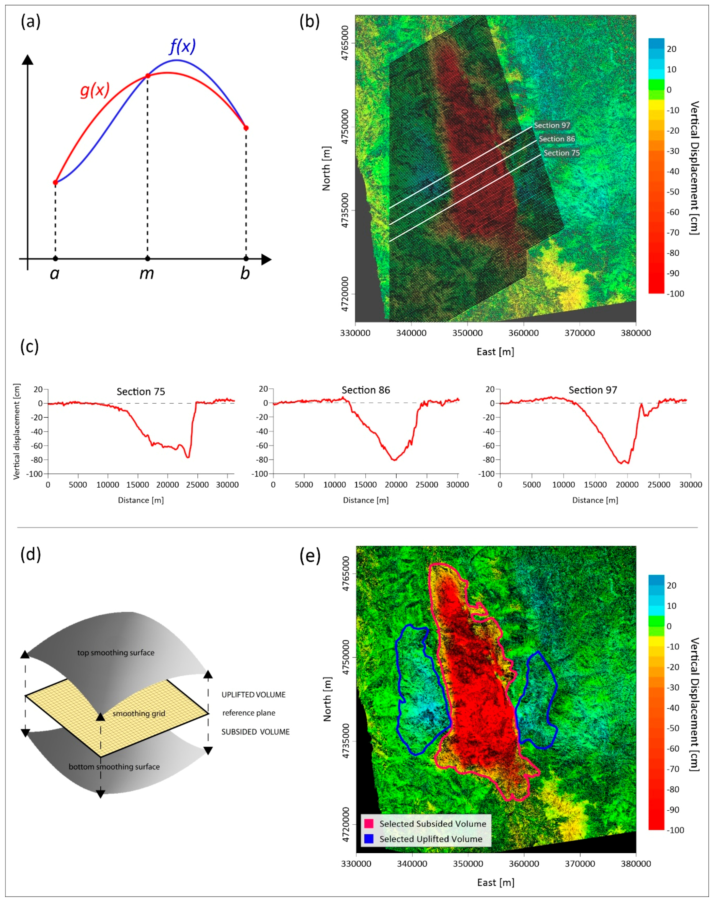
3.1. Topographic Method (3D Cavalieri–Simpson Modified Method)

This method is useful for numerical integration by using quadratic polynomials to approximate the integrand on a sequence of intervals [26]. This mathematical law envisages subdivision of the integration interval into sub-intervals, in which the function is integrated through parabolic arches (i.e., through quadrangular polynomials). Specifically, we produce a uniformed regular matrix of the ground deformation displacement maps, considering the Nearest Neighbour geostatistical gridding method. This method assigns the value of the nearest point to each grid node and is useful when data are already evenly spaced. Alternatively, in cases where the data are nearly on a grid with only a few missing values, this method is effective for filling in the holes in the data. On this vertical displacement map, we trace 192 profiles that spatially include both the subsided and the uplifted zones (Figure 4a–c). These profiles are spaced 250 m apart and the spacing is selected taking into account the maximum horizontal gradient of the vertical component of deformation. We firstly calculate the areas by considering each profile and, subsequently, we compute the subsided and the uplifted volumes by multiplying the computed areas times the distances.

3.2. Numerical Approach Method

This method allows us to calculate automatically volumes by using the Surfer 15^® tool (Golden Software, Golden, CO, USA). This software is able to realize this computational analysis considering solids defined by an upper surface and a lower one (we use again the Nearest Neighbour geostatistical gridding method) and employing three classical numerical integration algorithms [27]. These three mathematical methods can be recognized as:

• the Extended Trapezoidal Rule, represented by the following formula:

  $$Volume\approx \frac{\Delta y}{2}\left[A_1+2A_2+2A_3+4A_3+\dots +2A_{nCol-1}+A_{nCol}\right]$$

  (1)

  where ∆y is the grid row spacing and A is the area.
• the Extended Simpson’s Rule, represented by the following formula:

  $$Volume\approx \frac{\Delta y}{3}\left[A_1+4A_2+2A_3+4A_3+\dots +2A_{nCol-1}+A_{nCol}\right]$$

  (2)

  where ∆y is the grid row spacing and A is the area.
• the Extended Simpson’s 3/8 Rule, represented by the following formula:

  $$Volume\approx \frac{3\Delta y}{8}\left[A_1+3A_2+3A_3+2A_3+\dots +2A_{nCol-1}+A_{nCol}\right]$$

  (3)

  where ∆y is the grid row spacing and A is the area.

The difference in the volume calculations by three different methods measures the accuracy of the volume computations. We obtain very similar values and, therefore, we report in

Table 2. Results obtained by employing the three abovementioned methods.

Deformed Volume [km3]	Topographic Method	Numerical Approach Method	Surfacing Method
Subsidence	0.100	0.101	0.101
Uplift	0.0070	0.0074	0.0075
Unbalance	0.0930	0.0936	0.0935

the mean value obtained by using the abovementioned automatic approaches.

3.3. Surfacing Method

The starting point of this method is the separation of the DInSAR measurements into negative and positive components of the vertical displacement. The two obtained datasets are smoothed over a regular grid by the surface routine of the software Generic Mapping Tools [28,29] by solving:

$$\left(1-T\right)\ast \nabla \left(\nabla \left(z\right)\right)+T\ast \nabla \left(z\right)=0$$

(4)

where ∇ indicates the Laplacian operator, z is the vertical displacement value and T is a tension factor between 0 and 1. T = 0 gives the minimum curvature solution and T = 1 gives a harmonic surface (no maxima or minima are possible). We test all values for the T tension factor with no significant differences in obtained volumes, hence we hold T = 0.5 as suggested in Smith and Wessel [28] for steep topography data. We use a horizontal grid resolution of 5 × 5 cm even if results are stable increasing the grid resolution about one order. Two different surfaces, containing all positive (top smoothing surface) and negative (bottom smoothing surface) values respectively, are than defined (Figure 4d). Following, we select a subset of both datasets (positive/negative) by using location polygons enclosing uplifted and subsided areas, respectively, in both the hangingwall and footwall of the main fault (magenta and blue shaded areas in Figure 4e). Considering a reference plane located at 0 cm elevation (Figure 4d) and measuring the volume between the reference plane and the top smoothing surface, and between the reference plane and the bottom smoothing surface, we obtain the uplifted and the subsided volumes, respectively.

3.4. Results

The DInSAR measurements show that during the NEQ the hangingwall block was affected by broad subsidence with a maximum vertical amplitude of about 98 cm and by a significantly less extended region characterized by uplift (with a maximum of about 14 cm); moreover, also the footwall block was affected by uplift (with a maximum of about 10 cm; Figure 3b–e). The Topographic method shows that the NEQ was characterized by a subsided volume of 0.100 km³ while the uplifted volume was 0.0070 km³. By using the Numerical method, volumes of 0.101 km³ and 0.0074 km³ were calculated for subsidence and uplift, respectively. Finally, volumes of 0.101 km³ and 0.0075 km³ were obtained with the Surfacing method for subsidence and uplift, respectively. The very similar values obtained with these methods assess the reliability of our results. In addition, we remark that the subsided and uplifted rock volumes are markedly different and the unbalance (i.e., the difference between subsided and uplifted volumes) is 0.0930 km³, 0.0936 km³, and 0.0935 km³ for the Topographic, Numerical and Surfacing methods, respectively (Table 2).

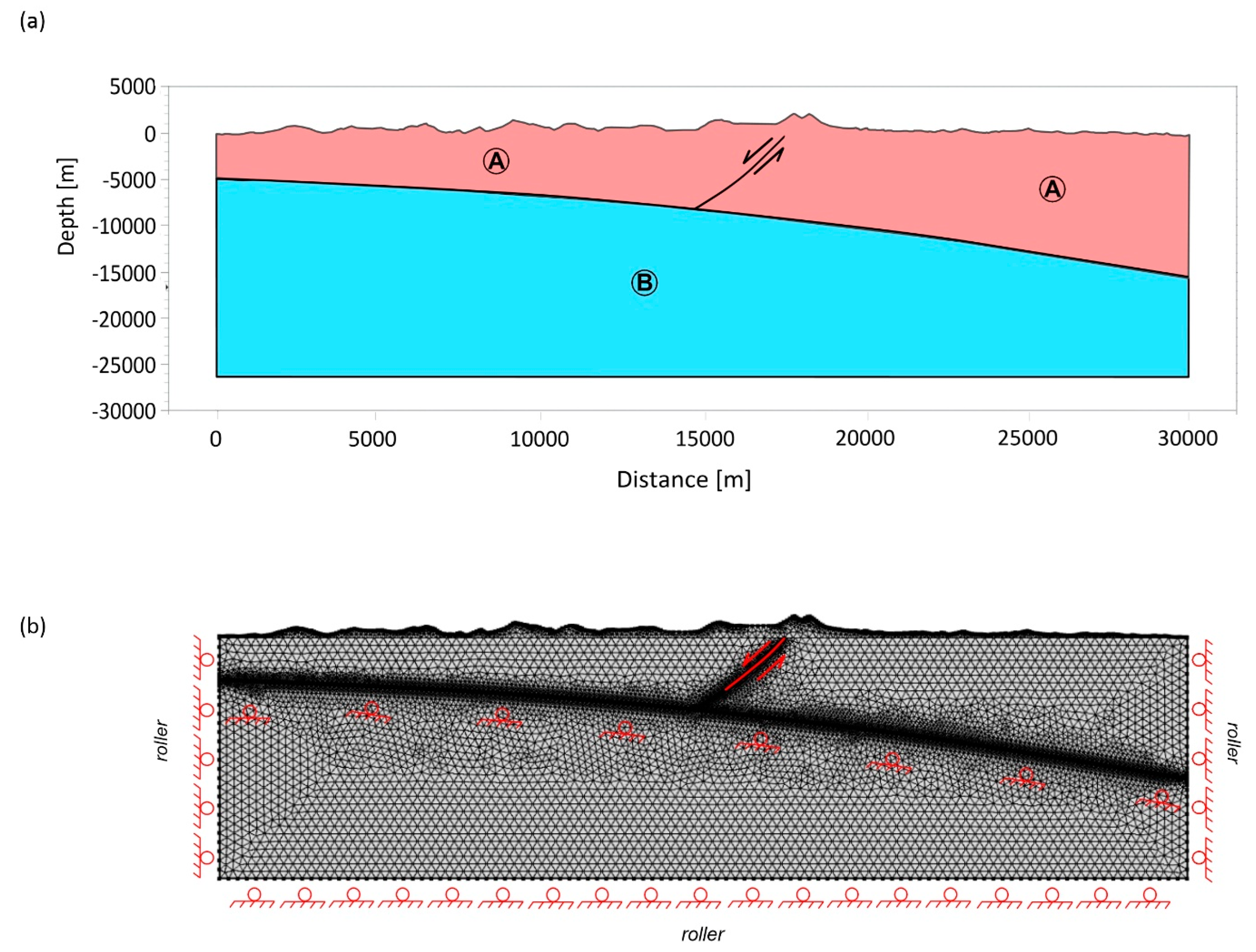
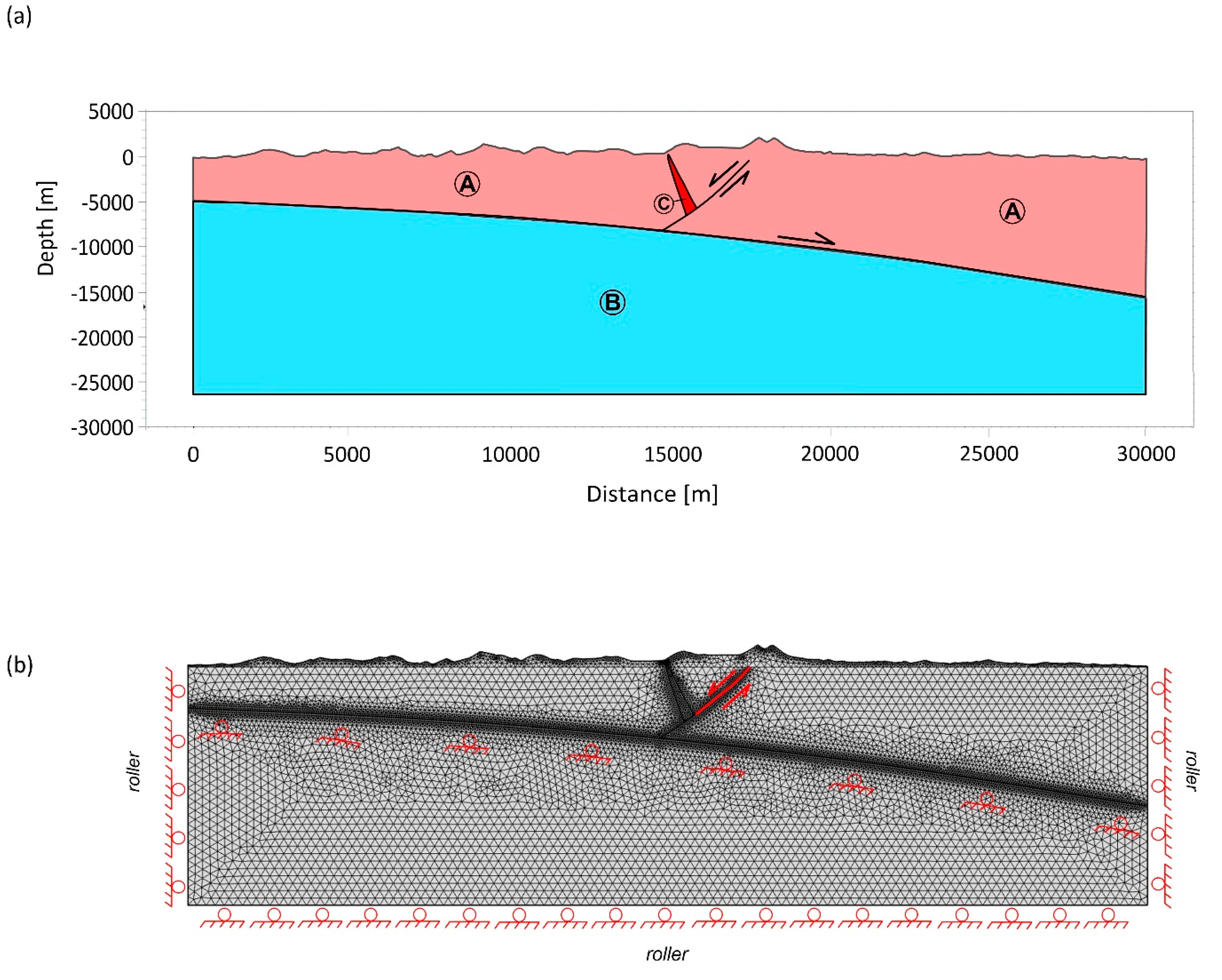
4. Numerical Modelling

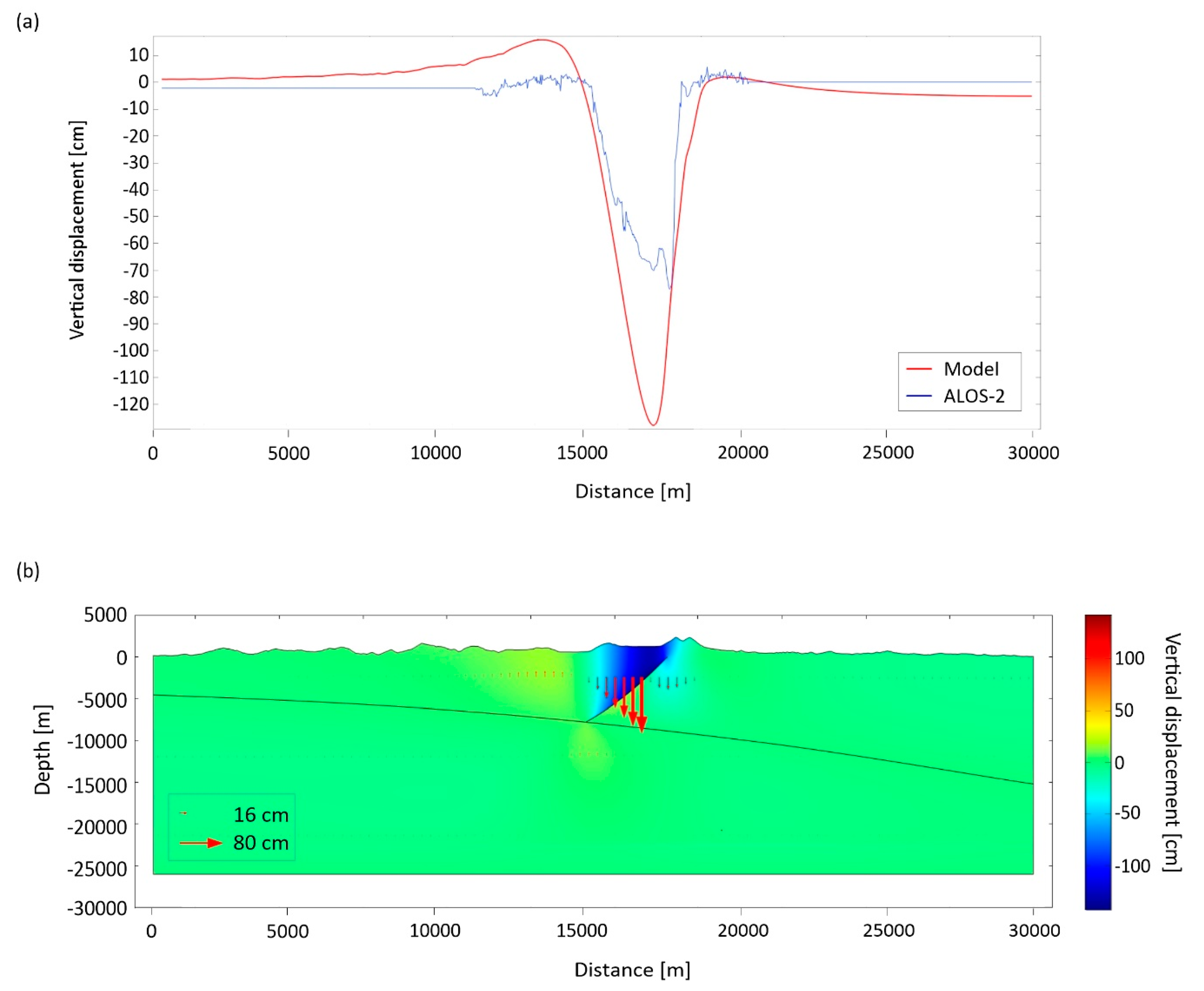
The results presented in the previous section clearly highlight an unbalance between the subsided and the uplifted volumes. To provide a possible interpretation of this volumetric asymmetry we propose a 2D numerical model of the NEQ based on the finite element method and implemented in a structural-mechanic framework (Figure 5, Figure 6, Figure 7 and Figure 8); our approach is based on the linear elasticity and on the plain strain approximation mode to minimize the differences between the modelled vertical displacements and those retrieved through the DInSAR analysis [30,31]. In particular, in the considered numerical environment we exploit the a priori available geological and structural information and the seismicity distribution relevant to the investigated seismogenic area, to take into account the mechanical heterogeneity and the active alignments that characterize the upper crust in the Apennines chain. According to Tizzani et al. [30], we evolve our model through two stages: during the first one (interseismic), the model compacts under the weight of the rock successions (gravity loading) until it reached a stable equilibrium. At this level, we consider only the retrieved tensional field while maintaining the total displacements equal to zero. At the second stage (co-seismic), where the stresses are instantaneously released through a no uniform slip along the faults, we use an iterative procedure based on a trial-and-error approach [32]. Starting from the geometry of the ground deformation pattern (see Figure 2) and to ensure the most representative section of this seismogenic area, we choose as reference profile the section BB’ (see Figure 1d and Figure 4c) reported in the maps of Figure 1b and Figure 4a. In this context, we build up a simplified geometry of the study region, which extends for about 100 km, with a depth of 26 km; such a large zone, with respect to the coseismic epicentral region, allows us to assume the edge effects as negligible (Figure 5a and Figure 7a). Concerning the lithological setting, we develop a heterogeneous model by considering two geological units having isotropic mechanical properties: (A) the Umbria-Marche carbonate sedimentary succession, (B) the evaporitic layer and basement unit (Figure 5a and Figure 7a) and a carbonate fractured unit (C in Figure 7a). The considered elastic parameters values are reported in

Table 3. Parameters for each layer defined in the model: Density (kg/m³), Young’s Modulus (GPa) and Poisson’s Ratio.

Parameters	Unit A	Unit B	Unit C
Density	2600	2700	2300
Young’s Modulus	30	30	9
Poisson’s Ratio	0.33	0.32	0.27

[33].

To simulate the possible structural frameworks of the investigated area, we defined two possible scenarios: (1) a single SW-dipping fault; (2) a single SW-dipping fault with an antithetic zone.

4.1. Single Fault

This scenario consists of a single SW-dipping fault and of a low-angle E-dipping fault (Figure 5a). As boundary conditions, we adopt a free boundary at the Earth surface, whose geometry is constrained by the topography of the considered area. A roller condition at the two sides and at the bottom boundary of the numerical domain is applied [30]. In addition, we assume specific internal boundary settings for the main structural alignments pattern in order to simulate the tectonic contacts among the achieved structural domains. Gravity is applied as a body force to all the elements and a constant density of 2600 kg·m⁻³ is assigned to all the elements of the Unit A, whereas a density of 2700 kg·m⁻³ is assigned to the Unit B (Table 3). The behavior of the SW-dipping fault is modelled as a contact body with frictional forces, while the low-angle E-dipping seismogenic layer is modelled as a roller constraint. Moreover, we apply a couple of forces to the two sides of the main SW-dipping fault (the considered fault segment is 8 km long); the forces applied to the internal and external sides of the fault surfaces are equal to 3.4 MPa and 2.3 MPa, respectively. The entire numerical domain is discretized in 17,226 tetrahedral elements with a higher refinement along the two main faults (Figure 5b). In order to reproduce the coseismic displacement along the fault, we assume the stationarity and linear elasticity of the involved materials by considering the solution of the equilibrium mechanical equations [34].

The retrieved best fit model, evaluated by considering the achieved minimum RMS value of the residuals (i.e., the difference between measured and modelled displacements), is reported in Figure 6a for the vertical deformation component. The performed solution, accounting also for the topography of the considered area, does not show a good spatial fit with the observed ground deformations, both in terms of shape and amplitude of the residual signal. In particular, the performed misfit analysis revealed rather high RMS values for the achieved residuals of the ALOS-2 DInSAR measurements (RMS = 12.42 cm).

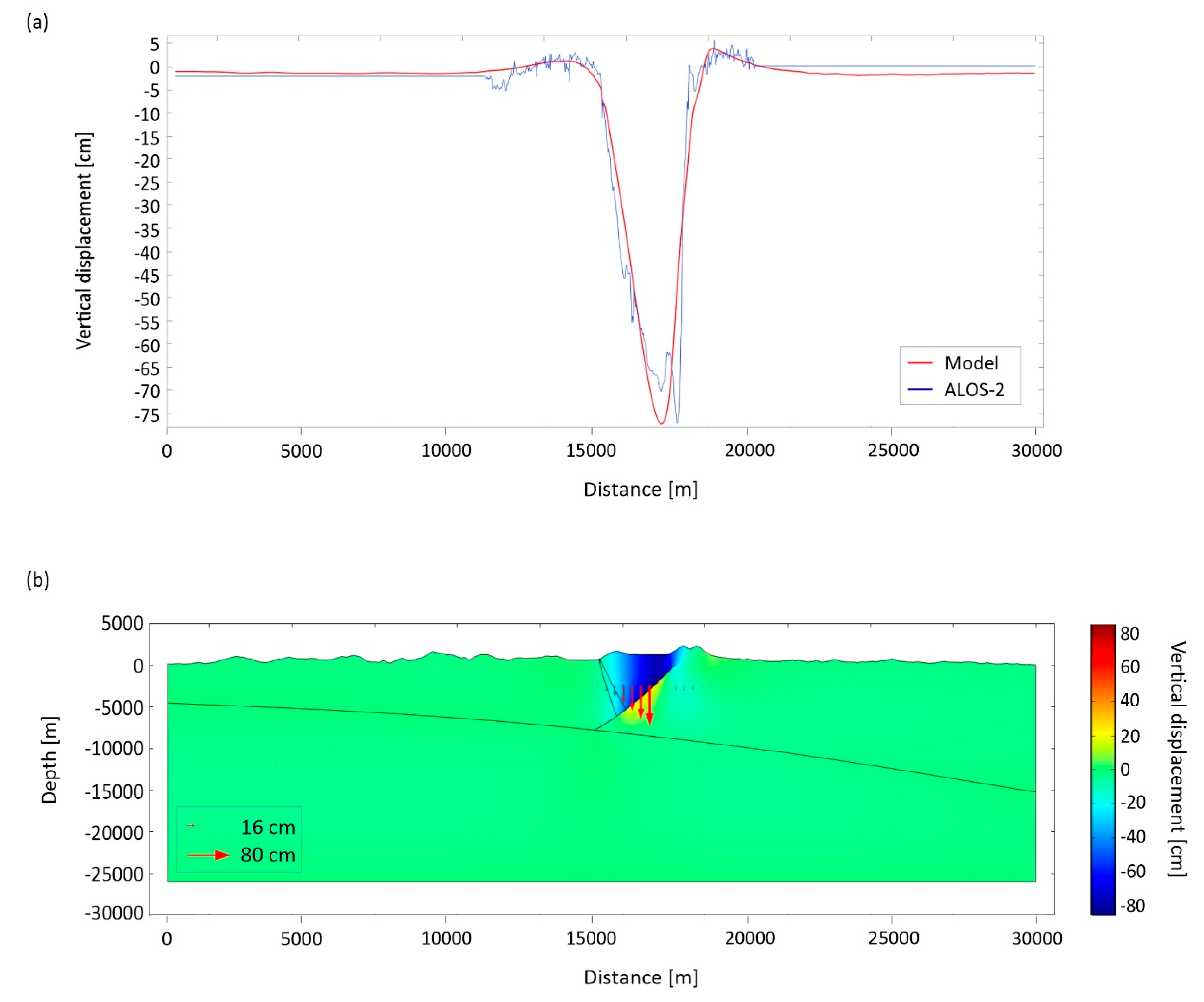
4.2. Antithetic Zone

This scenario consists of a single SW-dipping fault, of an antithetic fractured zone and of a low-angle E-dipping fault (Figure 7a). As boundary conditions, we adopt a free boundary at the Earth surface, whose geometry is constrained by the topography of the considered area. A roller condition at the two sides and at the bottom boundary of the numerical domain is applied [30]. In addition, we assume specific internal boundary settings for the main structural alignments pattern in order to simulate the tectonic contacts among the achieved structural domains. Also in this case, gravity is applied as a body force to all the elements. A constant density of 2600 kg·m⁻³ is assigned to all the elements of the Unit A, whereas density values of 2700 kg·m⁻³ and 2300 kg·m⁻³ are assigned to the Units B and C, respectively (Table 3). The behavior of the SW-dipping fault and of the antithetic zone is modelled as a contact body with frictional forces, while the low-angle E-dipping seismogenic layer as roller constraints. Moreover, we apply a couple of forces to the two sides of the main SW-dipping fault (the considered fault segment is 8 km long); the forces applied to the internal and external sides of the fault surfaces are equal to 3.4 MPa and 2.3 MPa, respectively. The entire numerical domain is discretized in 17,768 tetrahedral elements with a higher refinement along the three main structures (Figure 7b). In order to reproduce the coseismic displacement along the fault, we assume the stationarity and linear elasticity of the involved materials by considering the solution of the equilibrium mechanical equations [34].

Our best fit model, relevant to the minimum RMS value, is reported in Figure 8a for the vertical deformation component. The achieved solution, accounting also for the topography of the considered area, shows a very good fit with the observed ground deformations, both in terms of shape and amplitude of the residual signal. In particular, the performed misfit analysis revealed rather small RMS values for the achieved residuals of the ALOS-2 DInSAR measurements (RMS = 3.48 cm).

5. Discussion

We have extensively exploited seismological data and multi-orbit ALOS-2 DInSAR measurements relevant to the 30 October 2016 NEQ, to investigate the earthquake main surface deformation effects and the characteristics of the seismogenic source. The starting point of our study is the analysis of a set of ALOS-2 coseismic DInSAR maps, which reveals three distinct surface deformation patterns: (i) a major subsidence that reaches a maximum value of about 98 cm near the epicentral zones, nearby the town of Norcia; (ii) two smaller uplift lobes that affect both the hangingwall (reaching maximum values of about 14 cm) and the footwall blocks (reaching maximum values of about 10 cm; Figure 3b–e). Subsequently, we compute, by employing three different methods, the rock volumes affected by the retrieved uplift and subsidence effects during the NEQ. For all the methods, the coseismic uplift in the hangingwall block is about 1/14 of subsidence (Table 2), thus highlighting a significant volumetric asymmetry within the seismogenic crust. Following this analysis, we implement a numerical model of the NEQ which allows us to exploit the available geological and seismological data, and the ground deformation measurements retrieved from the multi-orbit DInSAR data. In particular, we investigate two different model scenarios obtained through the progressive integration of the a priori available information. First, we consider a more simplified scenario taking into account only the role of a single SW-dipping fault along which the M_w 6.5 NEQ nucleated. Subsequently, we implement a more realistic and complex scenario, characterized by a SW-dipping fault and an antithetic zone. We find that for the first scenario we cannot achieve a good fit with the observed ground deformations (RMS = 12.42 cm; Figure 7a,b); conversely, the second scenario furnishes a rather good fit with the coseismic surface deformation pattern (RMS = 3.48 cm; Figure 8a,b). Note that our modelling approach allows us to properly reproduce the retrieved ground deformation patterns through the combination of two different effects: (i) the gravitational sliding of the hangingwall along the main fault plane and (ii) the frictional force acting in the opposite direction, consistently with the double couple fault plane mechanism. These two effects are considered in both scenarios and, as already said, the second one, which consist of a SW-dipping fault and an antithetic zone, presents a rather good fit with the coseismic surface deformation pattern (Figure 8a,b). Therefore, we suggest that this second scenario represents a reliable one. In this case, two further elements are discussed in the following, which are relevant to the available seismological information and the retrieved rock volumes unbalance. For what concerns the signature of the antithetic zone, we remark that it is clearly visible through the hypocentral distribution of the earthquakes occurred between 24 August and 29 October 2016, showing an evident antithetic alignment; the seismicity data analysis suggests that the formation of this antithetic zone has already occurred before the NEQ nucleation (Figure 1c–f). Moreover, Porreca et al. [35] provided a novel reconstruction of the subsurface geology of the considered seismogenic area by using seismic reflection profiles. In particular, we take into account one of the interpreted sections in which the presence of an antithetic zone is clearly visible. Consequently, we analyze the temporal evolution of the occurred seismic events by combining and comparing their hypocentral locations with the abovementioned seismic profile, obtaining a good fitting. Finally, the distribution of the overall events of the seismic crisis and of those recorded since January 2015 also highlight the spatial position of the decollement layer.

As regards the retrieved volume unbalance, we underline that the processes that could promote such a permanent deformation within a rock mass are the diffusion mass transfer (i.e., pressure solution) and/or the plastic deformation (i.e., mineral recrystallization, grain boundary sliding). These processes are related to low strain rates phenomena occurring during interseismic phases, as also shown by field evidences [36] and laboratory simulations [37]. However, during the Norcia earthquake nucleation, we have retrieved a volume deficit in response to a high strain rate event. A possible explanation of this finding is based on the presence, at depth, of an interseismically dilated volume able to accommodate the collapse of a wedge bounded by the main fault, the antithetic one and a decollement layer. As proposed in Doglioni et al. [38], the hangingwall collapse can be allowed by the presence of a dilated zone, located antithetically to the main fault, generated from the decollement upward and that can absorb the volume settlement. When the strength of the fractured antithetic fault is not any able to sustain the weight of the rock wedge, the collapse of the hangingwall occurs in favor of gravity and the slip along the main fault allows the closure of the fractures generating the expulsion of the fluids [38]. In fact, we can interpret this volume as provided by microfractures filled by fluids circulating within the seismogenic crust; furthermore, their expulsion has been observed during the late pre-seismic and coseismic stage of the NEQ and could be related to the closure of this multitude of microfractures and by the consequent decrease during the earthquake of diffuse permeability [39]. We further remark that fluids expulsion phenomena are typical of extensional earthquakes such as the 1997 M_w 6.0 Colfiorito [40,41] and the 2009 M_w 6.3 L’Aquila earthquakes [42,43,44,45].

6. Conclusions

We have applied a multidisciplinary approach to study the 30 October 2016 M_w 6.5 Norcia (Central Italy) earthquake by exploiting the information derived from the hypocentral distribution of the occurred seismic events, the DInSAR measurements obtained from the ALOS-2 sensor, and numerical modelling. Our main findings can be summarized as follows:

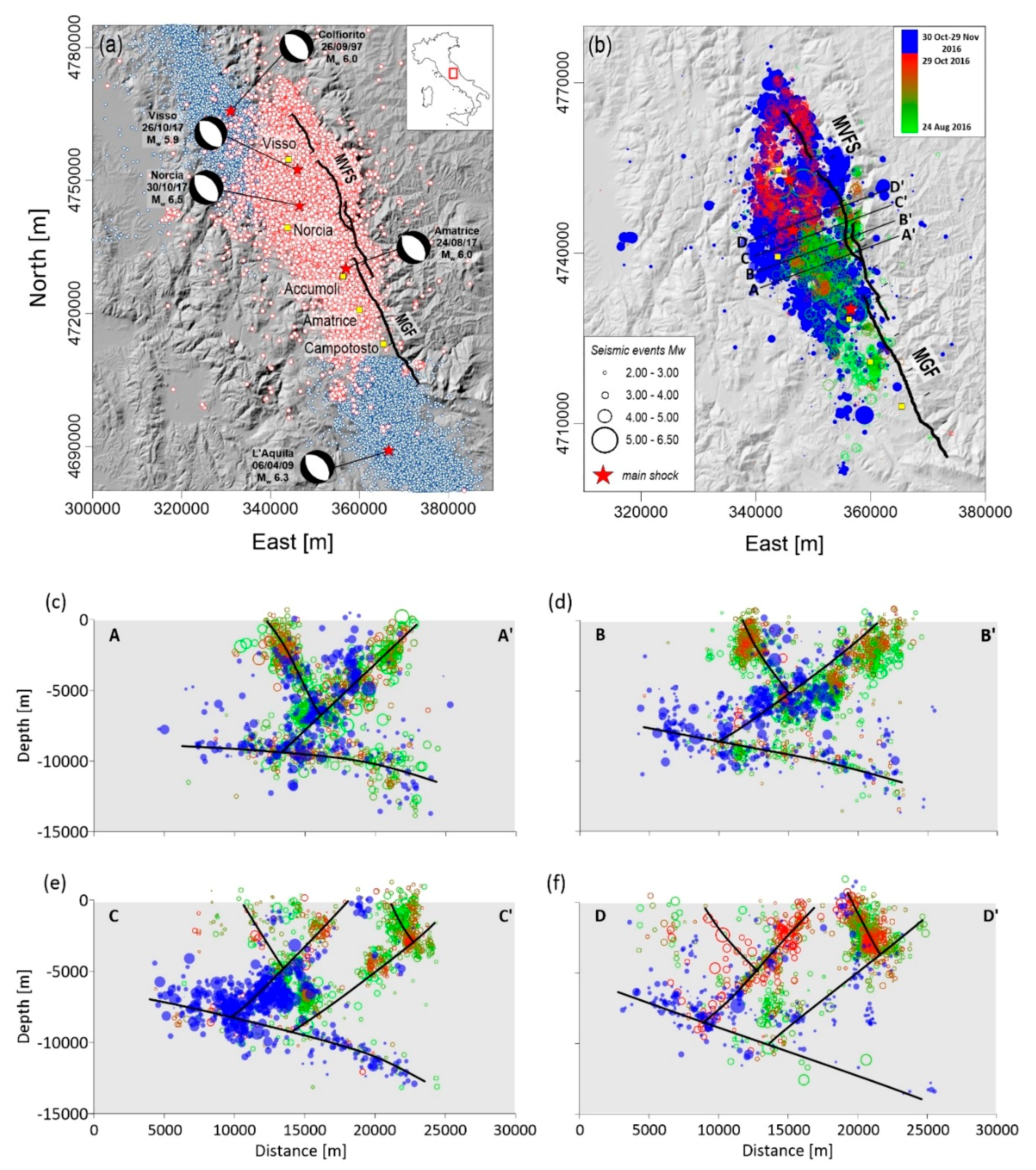
• the analysis of the relocated hypocenters allows us to highlight three main structures: (i) a SW-dipping alignment parallel to the main fault system; (ii) an E-dipping low-angle normal fault cutting through the upper crust; and (iii) ENE-dipping structures that are antithetic to the main fault;
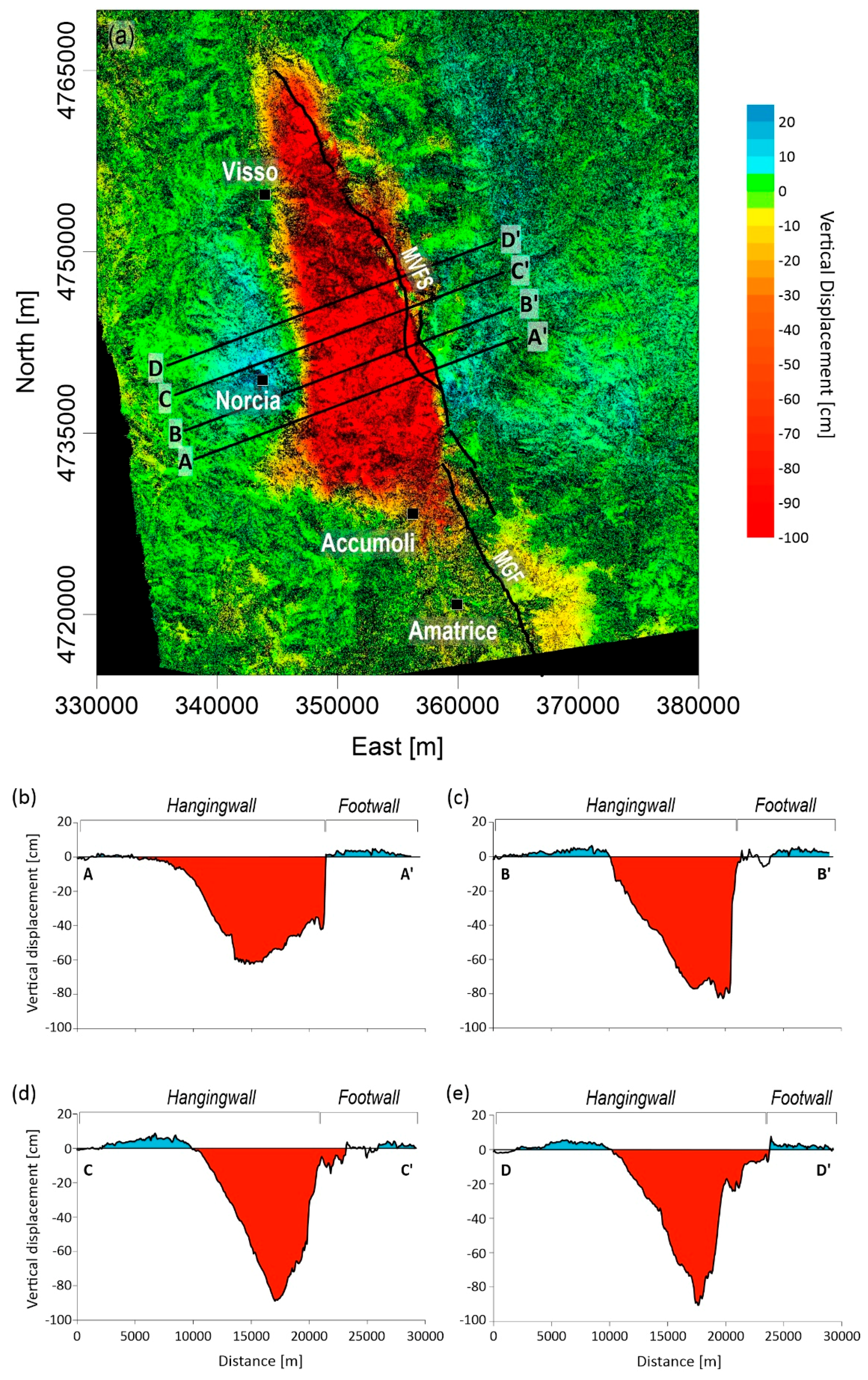
• the DInSAR measurements show that the considered seismogenic area was interested by significant coseismic ground deformations. The vertical displacement map shows three main deformation patterns: (i) a major subsidence that reaches a maximum value of about 98 cm near the epicentral zones, nearby the town of Norcia; (ii) two smaller uplift lobes that affect both the hangingwall (reaching maximum values of about 14 cm) and the footwall blocks (reaching maximum values of about 10 cm);
• the coseismic uplift in the hangingwall block is about 1/14 of subsidence, suggesting an unbalance between the subsided and the uplifted volumes within the seismogenic crust;
• the results of our 2D modelling highlight that the presence of an antithetic zone is necessary to reach the best fit between measured and simulated coseismic surface deformations (RMS = 3.48 cm). This result allows us to interpret the subsidence and uplift phenomena caused by the M_w 6.5 Norcia earthquake as the result of the gravitational sliding of the hangingwall along the main fault plane and the frictional force acting in the opposite direction, consistently with the double couple fault plane mechanism.

References

1. Chiarabba, C.; Jovane, L.; Di Stefano, R. A new view of Italian seismicity using 20 years of instrumental recordings. Tectonophysics 2005, 395, 251–268. [Google Scholar] [CrossRef]
2. Petricca, P.; Barba, S.; Carminati, E.; Doglioni, C.; Riguzzi, F. Graviquakes in Italy. Tectonophysics 2015, 656, 202–214. [Google Scholar] [CrossRef]
3. Lavecchia, G.; Castaldo, R.; de Nardis, R.; De Novellis, V.; Ferrarini, F.; Pepe, S.; Brozzetti, F.; Solaro, G.; Cirillo, D.; Bonano, M.; et al. Ground deformation and source geometry of the 24 August 2016 Amatrice earthquake (Central Italy) investigated through analytical and numerical modeling of DInSAR measurements and structural-geological data. Geophys. Res. Lett. 2016, 43. [Google Scholar] [CrossRef]
4. Cheloni, D.; De Novellis, V.; Antonioli, A.; Anzidei, M.; Atzori, S.; Avallone, A.; Bignami, C.; Bonano, M.; Calcaterra, S.; Castaldo, R.; et al. Geodetic model of the 2016 Central Italy earthquake sequence inferred from InSAR and GPS data. Geophys. Res. Lett. 2017, 44, 6778–6787. [Google Scholar] [CrossRef] [Green Version]
5. Thompson, G.A.; Parsons, T. From coseismic offsets to fault-block mountains. Proc. Nat. Acad. Sci. USA 2017, 114, 9820–9825. [Google Scholar] [CrossRef] [PubMed] [Green Version]
6. Galli, P.; Galadini, F.; Pantosti, D. Twenty years of paleoseismology in Italy. Earth Sci. Rev. 2008, 88, 89–117. [Google Scholar] [CrossRef]
7. Doglioni, C. A proposal for the kinematic modelling of W-dipping subductions-possible applications to the Tyrrhenian-Apennines system. Terra Nova 1991, 3, 423–434. [Google Scholar] [CrossRef]
8. Carminati, E.; Lustrino, M.; Doglioni, C. Geodynamic evolution of the central and western Mediterranean: Tectonics vs. igneous petrology constraints. Tectonophysics 2012, 579, 173–192. [Google Scholar] [CrossRef]
9. Chiaraluce, L. Unravelling the complexity of Apenninic extensional fault systems: A review of the 2009 L’Aquila earthquake (Central Apennines, Italy). J. Struct. Geol. 2012, 42, 2–18. [Google Scholar] [CrossRef]
10. Avallone, A.; Latorre, D.; Serpelloni, E.; Cavaliere, A.; Herrero, A.; Cecere, G.; D’Agostino, N.; D’Ambrosio, C.; Devoti, R.; Giuliani, R.; et al. Coseismic displacement waveforms for the 2016 August 24 Mw 6.0 Amatrice earthquake (central Italy) carried out from High-Rate GPS data. Ann. Geophys. 2016, 59. [Google Scholar] [CrossRef]
11. Wedmore, L.N.J.; Faure Walker, J.P.; Roberts, G.P.; Sammonds, P.R.; McCaffrey, K.J.W.; Cowie, P.A. A 667 year record of coseismic and interseismic Coulomb stress changes in central Italy reveals the role of fault interaction in controlling irregular earthquake recurrence intervals. J. Geophys. Res. Solid Earth 2017, 122, 5691–5711. [Google Scholar] [CrossRef]
12. Chiaraluce, L.; Amato, A.; Cocco, M.; Chiarabba, C.; Selvaggi, G.; Di Bona, M.; Piccinini, D.; Deschamps, A.; Margheriti, L.; Courboulex, F.; et al. Complex normal faulting in the Apennines thrust-and-fold belt: The 1997 seismic sequence in central Italy. Bull. Seism. Soc. Am. 2004, 94, 99–116. [Google Scholar] [CrossRef]
13. Chiaraluce, L.; Valoroso, L.; Piccinini, D.; Di Stefano, R.; De Gori, P. The anatomy of the 2009 L’Aquila norma fault system (central Italy) imaged by high resolution foreshock and aftershock locations. J. Geophys. Res. 2011, 116, B12311. [Google Scholar] [CrossRef]
14. Valoroso, L.; Chiaraluce, L.; Piccinini, D.; Di Stefano, R.; Schaff, D.; Waldhauser, F. Radiography of a normal fault system by 64,000 high-precision earthquake locations: The 2009 L’Aquila (central Italy) case study. J. Geophys. Res. Solid Earth 2013, 118, 1156–1176. [Google Scholar] [CrossRef]
15. Chiaraluce, L.; Di Stefano, R.; Tinti, E.; Scognamiglio, L.; Michele, M.; Casarotti, E.; Cattaneo, M.; De Gori, P.; Chiarabba, C.; Monachesi, G.; et al. The 2016 Central Italy seismic sequence: A first look at the mainshocks, aftershocks and source models. Seism. Res. Lett. 2017, 88, 757–771. [Google Scholar] [CrossRef]
16. Smeraglia, L.; Billi, A.; Carminati, E.; Cavallo, A.; Doglioni, C. Field-to nano-scale evidence for weakening mechanisms along the fault of the 2016 Amatrice and Norcia earthquakes, Italy. Tectonophysics 2017, 712–713, 156–169. [Google Scholar] [CrossRef]
17. Liu, C.; Zheng, Y.; Xie, Z.; Xiong, X. Rupture features of the 2016 Mw 6.2 Norcia earthquake and its possible relationship with strong seismic hazards. Geophys. Res. Lett. 2017, 44, 1320–1328. [Google Scholar] [CrossRef]
18. Pizzi, A.; Di Domenica, A.; Gallovič, F.; Luzi, L.; Puglia, R. Fault segmentation as constraint to the occurrence of the main shocks of the 2016 Central Italy seismic sequence. Tectonics 2017, 36, 2370–2387. [Google Scholar] [CrossRef]
19. Xu, G.; Xu, C.; Wen, Y.; Jiang, G. Source Parameters of the 2016–2017 Central Italy Earthquake Sequence from the Sentinel-1, ALOS-2 and GPS Data. Remote Sens. 2017, 9, 1182. [Google Scholar] [CrossRef]
20. Scognamiglio, L.; Tinti, E.; Casarotti, E.; Pucci, S.; Villani, F.; Cocco, M.; Magnoni, F.; Michelini, A.; Dreger, D. Complex fault geometry and rupture dynamics of the Mw 6.5, 2016, October 30th central Italy earthquake. J. Geophys. Res. Solid Earth 2018. [Google Scholar] [CrossRef]
21. Barchi, M.R.; Alvarez, W.; Shimabukuro, D.H. The Umbria-Marche Apennines as a Double Orogen: Observations and hypotheses. Ital. J. Geosci. 2012, 131, 258–271. [Google Scholar] [CrossRef]
22. Boncio, P.; Lavecchia, G.; Milana, G.; Rozzi, B. Seismogenesis in Central Apennines, Italy: An integrated analysis of minor earthquake sequences and structural data in the Amatrice-Campotosto area. Ann. Geophys. 2004, 47, 1723–1742. [Google Scholar]
23. Galadini, F.; Galli, P. Paleoseismology of silent faults in the Central Apennines (Italy): The Mt. Vettore and Laga Mts. Faults. Ann. Geophys. 2003, 46, 815–836. [Google Scholar]
24. Costantini, M. A novel phase unwrapping method based on network programming. IEEE Trans. Geosci. Remote Sens. 1998, 36, 813–821. [Google Scholar] [CrossRef]
25. Manzo, M.; Ricciardi, G.P.; Casu, F.; Ventura, G.; Zeni, G.; Borgström, S.; Berardino, P.; Del Gaudio, C.; Lanari, R. Surface deformation analysis in the Ischia Island (Italy) based on spaceborne radar interferometry. J. Volcanol. Geoth. Res. 2006, 151, 399–416. [Google Scholar] [CrossRef]
26. Velleman, D.J. The generalized Simpson’s rule. Am. Math. Mon. 2005, 112, 342–350. [Google Scholar] [CrossRef]
27. Press, W.H.; Flannery, B.P.; Teukolsky, S.A.; Vetterling, W.T. Numerical Recipes in C; Cambridge University Press: Cambridge, UK, 1988. [Google Scholar]
28. Smith, W.H.F.; Wessel, P. Gridding with continuous curvature splines in tension. Geophysics 1990, 55, 293–305. [Google Scholar] [CrossRef]
29. Wessel, P.; Smith, W.H.F.; Scharroo, R.; Luis, J.F.; Wobbe, F. Generic Mapping Tools: Improved version released. EOS Trans. AGU 2013, 94, 409–410. [Google Scholar] [CrossRef]
30. Tizzani, P.; Castaldo, R.; Solaro, G.; Pepe, S.; Bonano, M.; Casu, F.; Manunta, M.; Manzo, M.; Pepe, A.; Samsonov, S.; et al. New insights into the 2012 Emilia (Italy) seismic sequence through advanced numerical modeling of ground deformation InSAR measurements. Geophys. Res. Lett. 2013, 40, 1971–1977. [Google Scholar] [CrossRef] [Green Version]
31. Castaldo, R.; de Nardis, R.; DeNovellis, V.; Ferrarini, F.; Lanari, R.; Lavecchia, G.; Pepe, S.; Solaro, G.; Tizzani, P. Coseismic Stress and Strain Field Changes Investigation Through 3-D Finite Element Modeling of DInSAR and GPS Measurements and Geological/Seismological Data: The L’Aquila (Italy) 2009 Earthquake Case Study. J. Geophys. Res. Solid Earth 2018, 123, 4193–4222. [Google Scholar] [CrossRef]
32. Tarantola, A. Inverse Problem Theory and Methods for Model Parameter Estimation; SIAM Society for Industrial and Applied Mathematics: Philadelphia, PA, USA, 2005; ISBN 0-89871-572-5. [Google Scholar]
33. Schön, J.H. Physical Properties of Rocks: Fundamentals and Principles of Petrophysics; Elsevier: Amsterdam, The Netherlands, 2015; Volume 65. [Google Scholar]
34. Fagan, M.J. Finite Elements Analysis: Theory and Practice; Prentice Hall: Upper Saddle River, NJ, USA, 1992; pp. 1–311. [Google Scholar]
35. Porreca, M.; Minelli, G.; Ercoli, M.; Brobia, A.; Mancinelli, P.; Cruciani, F.; Giorgetti, C.; Carbomi, F.; Mirabella, F.; Cavinato, G.; et al. Seismic Reflection Profiles and Subsurface Geology of the Area Interested by the 2016–2017 Earthquake Sequence (Central Italy). Tectonics 2018, 37, 1116–1137. [Google Scholar] [CrossRef]
36. Gratier, J.P.; Thouvenot, F.; Jenatton, L.; Tourette, A.; Doan, M.L.; Renard, F. Geological control of the partitioning between seismic and aseismic sliding behaviours in active faults: Evidence from the Western Alps, France. Tectonophysics 2013, 600, 226–242. [Google Scholar] [CrossRef]
37. Tesei, T.; Collettini, C.; Barchi, M.R.; Carpenter, B.M.; Di Stefano, G. Heterogeneous strength and fault zone complexity of carbonate-bearing thrusts with possible implications for seismicity. Earth Plan. Sci. Lett. 2014, 408, 307–318. [Google Scholar] [CrossRef]
38. Doglioni, C.; Carminati, E.; Petricca, P.; Riguzzi, F. Normal fault earthquakes or graviquakes. Sci. Rep. 2015, 5. [Google Scholar] [CrossRef] [PubMed]
39. Barberio, M.D.; Barbieri, M.; Billi, A.; Doglioni, C.; Petitta, M. Hydrogeochemical changes before and during the 2016 Amatrice-Norcia seismic sequence (central Italy). Sci. Rep. 2017, 7. [Google Scholar] [CrossRef] [PubMed] [Green Version]
40. Quattrocchi, F.; Pik, R.; Pizzino, L.; Guerra, M.; Scarlato, P.; Angelone, M.; Barbieri, M.; Conti, A.; Marty, B.; Sacchi, E. Geochemical changes at the Bagni di Triponzo thermal spring during the Umbria-Marche 1997–1998 seismic sequence. J. Seism. 2000, 4, 567–587. [Google Scholar] [CrossRef]
41. Carro, M.; De Amicis, M.; Luzi, L. Hydrogeological changes related to the Umbria–Marche earthquake of 26 September 1997 (Central Italy). Nat. Hazards 2005, 34, 315–339. [Google Scholar] [CrossRef]
42. Di Luccio, F.; Ventura, G.; Di Giovambattista, R.; Piscini, A.; Cinti, F.R. Normal faults and thrusts re-activated by deep fluids: The 6 April 2009 Mw 6.3 L’Aquila earthquake, central Italy. J. Geophys. Res. 2010, 115, B06315. [Google Scholar] [CrossRef]
43. Terakawa, T.; Zoporowski, A.; Galvan, B.; Miller, S.A. High-pressure fluid at hypocentral depths in the L’Aquila region inferred from earthquake focal mechanisms. Geology 2010, 38, 995–998. [Google Scholar] [CrossRef]
44. Doglioni, C.; Barba, S.; Carminati, E.; Riguzzi, F. Fault on–off versus coseismic fluids reaction. Geosci. Front. 2014, 5, 767–780. [Google Scholar] [CrossRef]
45. Sugan, M.; Kato, A.; Miyake, H.; Nakagawa, S.; Vuan, A. The preparatory phase of the 2009 Mw 6.3 L’Aquila earthquake by improving the detection capability of low-magnitude foreshocks. Geophys. Res. Lett. 2014, 41, 6137–6144. [Google Scholar] [CrossRef]
Figure 1. Seismological scenario. (a) Seismicity distribution in Central Italy recorded from 24 August to 29 November 2016 (red circles) [15], superimposed on the 1 arcsec Shuttle Radar Topography Mission (SRTM) Digital Elevation Model (DEM) of the zone: the 1997–1998 Colfiorito and the 2009 L’Aquila seismic sequences are also shown (blue dots). The seismic events with Mw ≥ 5.4 are represented by red stars and the associated focal mechanisms are also reported in the map. The black lines represent the main faults located in this area: the Mt. Gorzano Fault (MGF) and the Mt. Vettore Fault System (MVFS); (b) Seismicity distribution as a function of magnitude (the higher the magnitude, the bigger the circles) and day of occurrence (from green to red circles). The seismic events with Mw ≥ 5.4 are also indicated and are represented by red stars. The black lines represent the section profiles reported in panels (be), in which the relocated hypocenters of the occurred earthquakes and the main inferred geological alignments (black lines) are projected.
Remotesensing 10 01901 g001
Figure 2. DInSAR analysis. (a,b) DInSAR (Line-of-sight [LOS]) displacement maps computed by using ALOS-2 images acquired from: (a) ascending orbits on 24 August–2 November 2016 and (b) descending orbits on 31 August–9 November 2016; (c) vertical displacement map computed by exploiting the ascending and descending ALOS-2 measurements shown in panels (a,b), and including both the Mw 5.9 Visso and the Mw 6.5 Norcia earthquakes. The magenta rectangle indicates the area considered in Figure 3a; (d) E-W displacement map computed by exploiting the ascending and descending ALOS-2 measurements shown in panels (a,b), and including both the effect of the Mw 5.9 Visso and the Mw 6.5 Norcia earthquakes. The white star represents the Mw 6.5 Norcia mainshock. The white and black lines represent the contour lines of the maximum deformation zones and the main faults located in this area (i.e., MGF and MVFS), respectively.
Remotesensing 10 01901 g002
Figure 3. Vertical displacement analysis. (a) Vertical displacement map of Figure 2c with superimposed the black lines representing the main structural alignments located in this area. Moreover, the black lines represent the traces of the displacement profiles reported in panels (be), in which the subsided and the uplifted volumes are highlighted in red and light blue, respectively.
Remotesensing 10 01901 g003
Figure 4. Volume retrieval methods. (a) Graphical representation of the Cavalieri-Simpson Rule; this method approximates the integral of the requested function (in blue) with that of the parabola that interpolates it in the nodes (in red); (b) Vertical component map in which the exploited 192 traced profiles are reported; (c) Examples of the displacement profiles (in red) used for the volumes computation; (d) Graphic representation of the Surfacing Method. The employed routine is able to calculate the uplifted and subsided volumes, considering a reference plane located at 0 cm elevation and measuring the volume between the reference plane and the top smoothing surface, and between the reference plane and the bottom smoothing surface, respectively; (e) Vertical component map in which the polygons used for the computation of the subsided (in magenta) and uplifted (blue) volumes are shown.
Remotesensing 10 01901 g004
Figure 5. Single fault model setup. (a) Simplified geological cross-section (BB’ reported in Figure 1d and Figure 4c) exploited in the considered FE environment; (b) Discretized numerical domains with highlighted the boundary conditions; note that the red line represent the segments along which the forces are applied.
Remotesensing 10 01901 g005
Figure 6. Results of the single fault model. (a) Comparison between the vertical component of the deformations retrieved through the DInSAR analysis and the FE modelling; (b) Crustal distribution of the modelled vertical components of the retrieved displacements; the red arrows indicate the modelled displacement vectors.
Remotesensing 10 01901 g006
Figure 7. SW-dipping fault and antithetic zone model setup. (a) Simplified geological cross-section (BB’ reported in Figure 1d and Figure 4c) exploited in the considered FE environment; (b) Discretized numerical domains with highlighted the boundary conditions; note that the red line represents the segments along which the forces are applied.
Remotesensing 10 01901 g007
Figure 8. Results of the SW-dipping fault and antithetic zone model. (a) Comparison between the vertical component of the deformations retrieved through the DInSAR analysis and the FE modelling; (b) Crustal distribution of the modelled vertical components of the retrieved displacements; the red arrows indicate the modelled displacement vectors.
Remotesensing 10 01901 g008