A Methodological Framework to Retrospectively Obtain Downscaled Precipitation Estimates over the Tibetan Plateau

Abstract

Long-term precipitation estimates with both finer spatial resolution and better quality are vital and highly needed in various related fields. Numerous downscaling algorithms have been investigated based on the Tropical Rainfall Measuring Mission (TRMM) Multi-Satellite Precipitation Analysis (TMPA), to obtain precipitation data with finer resolution (~1 km). However, this research was restricted by the time span of the TMPA dataset, as the starting time of TMPA was 1998. In this study, a new methodological framework incorporating wavelet coherence and Cubist was proposed to retrospectively obtain downscaled precipitation estimates (DS) over the Tibetan Plateau (TP), based on TMPA and ground observations, in 1990s. The correlations and similarities of precipitation patterns between the target years, from 1990 to 1999, and reference years, from 2000 to 2013, were firstly determined using wavelet coherence based on ground observations. Following this, the TMPA data in the reference years were regarded as the reference in the corresponding target years, which were adopted to be downscaled using Cubist models and land surface variables, to obtain the DS in the target years. We found that the DS showed continuous trends, which corresponded well with the ground observations. Additionally, the performances of the DS were better than those of the Climate Hazards group Infrared Precipitation with Stations (CHIRPS) data over the TP. Therefore, this methodological framework has great potential for obtaining precipitation estimates for the period of the 1990s for which TMPA data is inaccessible.

1. Introduction

Precipitation is commonly regarded as one of the most important variables in hydrology, meteorology, climate change, etc. [1]. Therefore, long-term precipitation information is in great need in related scientific and application fields. It is a great challenge to monitor and measure precipitation amounts and trends in particular in areas with complex terrain, for instance the Tibetan Plateau (TP). TP is the largest plateau in the world with an average elevation of >4000 m [2], which has also been identified as the pilot region to study climate fluctuations in the world due to its sensitivity to climate change. The temperature in TP has been rising since the 1950s [3], and precipitation shows an increasing trend since the 1990s [4]. However, the rain gauge network is significantly scarce over the TP due to its harsh environment and complex terrain [5], which makes it difficult to obtain spatially explicit precipitation information over the plateau. Additionally, strong variability in physiography can lead to localized variations in climatic conditions, needing much more information on the critical climatic variables, i.e., precipitation. Therefore, to investigate the regional climate fluctuations in the TP, long-term precipitation estimates with both finer resolutions (~1 km) and better accuracy are in great need.

Conventional point-based spatial interpolations using rain gauge measurements are used to generate high spatial resolution precipitation datasets. However, complex topography with sparse rain gauges often causes large uncertainties and errors in obtaining precipitation information using spatial interpolations [6]. Meanwhile, ground-based radar is spatially limited and practically useless over the TP. Thus, satellite-based precipitation products become the optimum source for providing precipitation estimates with larger spatial coverage. Satellite-based precipitation products, such as the Tropical Rainfall Measurement Mission (TRMM) Multi-Satellite Precipitation Analysis (TMPA) dataset, were extensively used over the past two decades. The TMPA data provides valuable precipitation information in areas with sparse rain gauges. However, coarse spatial resolution (0.25°) of the TMPA data restricts its application at the regional and basin scales [7]. To obtain precipitation estimates with finer spatial resolutions, numerous downscaling algorithms combining a suite of environmental variables have been investigated [8,9,10,11]. The Normalized Difference Vegetation Index (NDVI) was firstly employed to build exponential relationships with TMPA data [8]. Considering the effects of topography, regression kriging to establish predictive models based on the digital elevation model (DEM) was developed by [9]. In [10], both the NDVI and DEM were introduced in a multiple liner regression model to downscale TMPA data. Furthermore, [11] proposed a geographically weighted regression (GWR) model using both the NDVI and DEM. Meanwhile, other studies have demonstrated how various land surface characteristics, such as land surface temperature (LST) [12], topographical factors [13,14], influenced the spatial distribution of precipitation. Therefore, Ma et al. [15,16] incorporated a series of land surface variables, including NDVI, DEM, LST and other topographical factors, into a spatial data mining algorithm in order to downscale TMPA data.

Nevertheless, all these downscaling approaches based on TMPA data were restricted by the time span after 1998, due to the availability of TMPA data, thereby missing information from a very important period in investigating climate variability in the TP. For example, precipitation was reported to show an increasing trend in TP since the 1990s. Thus, obtaining precipitation estimates at fine spatial resolutions (~1 km) before the TMPA launch are critical, calling for new approaches.

This study intended to develop a new methodological framework, which incorporated wavelet coherence and Cubist, to retrospectively obtain downscaled precipitation estimates (DS) over the TP, based on TMPA data and ground observations, in the 1990s. Firstly, wavelet coherence is a powerful approach to detect the inherent similarities and correlations of precipitation between the target time periods, from 1990 to 1999, and the reference time periods, from 2000 to 2013, at different temporal scales based on ground observations [17,18,19]. Then, the TMPA data in the reference years were regarded as the reference in the corresponding target years, which were adopted to be downscaled using Cubist, a spatial data mining algorithm, to obtain the DS in the target years. The main objectives of this study were: (1) to develop a methodological framework to retrospectively obtain DS in the 1990s over the TP; (2) to evaluate the performance of the DS against ground observations; and (3) to compare the performance of the DS with those of the Climate Hazards group Infrared Precipitation with Stations (CHIRPS) data.

2. Materials and Methods

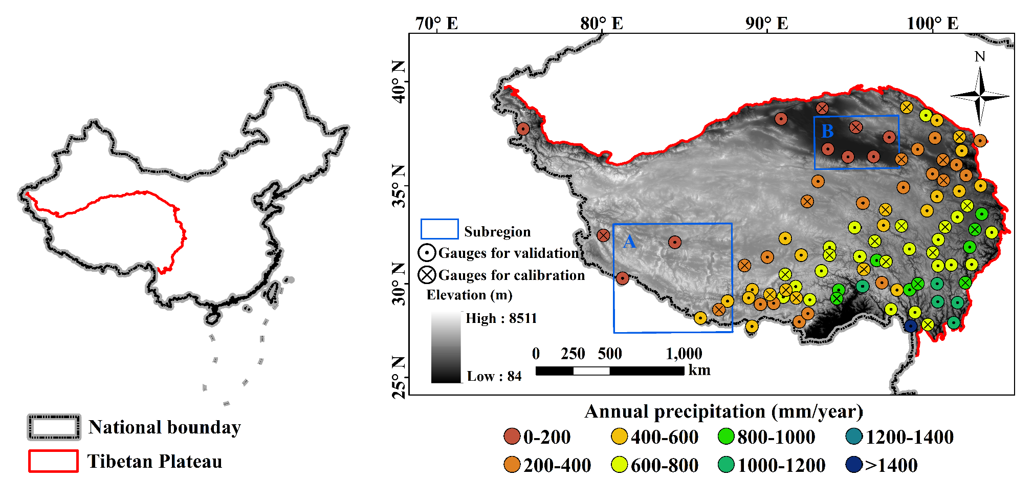
2.1. Study Area

The TP, formed after the collisions between the Indian plate and Eurasian continent plate, is the largest and highest plateau in the world, with a mean elevation above 4000 m (Figure 1). Due to its unique topography and location, the TP has complex climatic conditions [20]. Two main atmospheric circulation patterns affect the TP [21]. For instance, the Indian monsoons prevails in the central and southern parts of the plateau, leading to relatively larger precipitation in these regions (>1000 mm/year) in summer. While in the northern and western parts, which are mainly influenced by westerlies in winter, smaller precipitation occurs (<200 mm/year). Additionally, there is a clear demarcation between dry and wet seasons; about 90% of total annual precipitation occurs during the rainy season (mainly from March to August) [14].

2.2. Materials

2.2.1. Ground Observations

The annual precipitation records from 1954 to 2013 were provided by the China Meteorological Administration (http://data.cma.cn/). The working meteorological stations available over the TP were sparse and uneven due to the complex terrain and harsh environmental conditions (Figure 1). Most of the stations are located in the south and east parts of TP, and mainly at mid /low elevations.

2.2.2. Tropical Rainfall Measuring Mission (TRMM) Multi-Satellite Precipitation Analysis (TMPA) Dataset

Through the joint efforts of the National Aeronautics and Space Administration (NASA) and the Japan Aerospace Exploration Agency (JAXA), TRMM was successfully launched in November 1997. TRMM was equipped with instruments including the Visible and Infrared Scanner, TRMM Microwave Imager (TWI) and Precipitation Radar (PR), which was mainly designed to investigate precipitation intensity and distribution in subtropical and tropical regions. The TMPA 3B43 provides monthly precipitation estimates over regions spanning from $50°\mathrm{S}\mathrm{to}50°\mathrm{N}$ at the spatial resolution of 0.25$°$ [22]. The TMPA 3B43 dataset between 2000 and 2013 were employed in this study, which can be downloaded from https://pmm.nasa.gov/data-access/downloads/trmm.

2.2.3. The Climate Hazards group Infrared Precipitation with Stations (CHIRPS)

The Climate Hazards group Infrared Precipitation with Stations (CHIRPS) is a new quasi-global (50°S–50°N), high-resolution (~$0.05°$) precipitation dataset with several temporal scales (daily, pentadal and monthly). The CHIRPS data uses the TMPA 3B42 version 7 to calibrate global Cold Cloud Duration (CCD) rainfall estimates and blends precipitation observations from a variety of sources including national and regional meteorological services [23,24]. The spatial resolution of CHIRPS is higher than other satellite-based global precipitation datasets, making it favorable to analyze precipitation variations at finer scales. In this study, monthly data from the CHIRPS database for the period from January 1990 to December 1999 are employed (ftp://ftp.chg.ucsb.edu/pub/org/chg/products/CHIRPS-2.0).

2.2.4. Normalized Difference Vegetation Index (NDVI) Dataset

NDVI is commonly applied to depict the productivity and distribution of vegetation [25,26]. The relationships between NDVI and precipitation were extensively investigated by various researchers [15,27,28]. The NDVI datasets were obtained from two satellite-based products: (1) for the period from 1990 to 1999, the dataset was obtained from the Global Inventory Monitoring and Modeling System (GIMMS-NDVI3g). The GIMMS produced the global NDVI dataset using the information collected from the Advanced Very High Resolution Radiometer (AVHRR) sensors. The latest version of GIMMS-NDVI3g (3g. v1) has a spatial resolution of $1/12°\times 1/12°,$ which can be found at https://ecocast.arc.nasa.gov/data/pub/gimms/3g.v1/. (2) For the period from 2000 to 2013, the dataset was collected from Moderate Resolution Imaging Spectroradiometer (MODIS). MOD13A2 is a NDVI dataset at 1 km spatial resolution and was obtained from https://ladsweb.modaps.eosdis.nasa.gov/search/.

2.2.5. Land Surface Temperature (LST) Datasets

Two types of land surface temperature (LST) datasets were used in this study. MODIS provided LST records worldwide with an error controlled between −1 K and 1 K. The MOD11A2 products, which produced LST and Emissivity data at 1 km spatial resolution over every eight days, were used in this study for the period between 2000 and 2013.

LST data from 1990 to 1999 was estimated using the split window method following [29].

$$t_s=0.32{\left(t_4-t_5\right)}^2+1.40\left(t_4-t_5\right)+t_4+\left(57-5w\right)\left(1-\mathsf{\epsilon }\right)-\left(161-30w\right)\Delta \mathsf{\epsilon }+0.83$$

(1)

where $t_4$ and $t_5$ were the radiometric temperatures in channel 4 (10.3 to 11.3 $\mathsf{\mu }\mathrm{m}$) and channel 5 (11.5 to 12.5 $\mathsf{\mu }\mathrm{m}$) of the AVHRR sensor, respectively. w represented the volume of water vapor in the atmosphere, $\mathsf{\epsilon }$ was calculated by averaging the emissivity for channels 4 and 5, and $\Delta \mathsf{\epsilon }$ denoted the differences of emissivities between channels 4 and 5. The estimate errors of LST generated by split window could be controlled at ~$\pm$1 K compared to in situ data [30,31]. Meanwhile, the LST estimates by split window also showed good agreement with those based on MODIS LST algorithm [32,33]. The spatial resolution of the processed LST data using split window was approximately 1.1 km at the annual scale.

2.2.6. Topography Datasets

The Shuttle Radar Topography Mission (SRTM) project, cooperated between NASA and the National Geospatial-Intelligence Agency (NGA), was successfully launched in February 2000. The SRTM project provided high-resolution DEM data with a spatial coverage ranging from 56°S to 60°N. The 3 arc–second (approximately 90 m) grid DEM was obtained from http://srtm.csi.cgiar.org and used in this study.

2.3. Methods

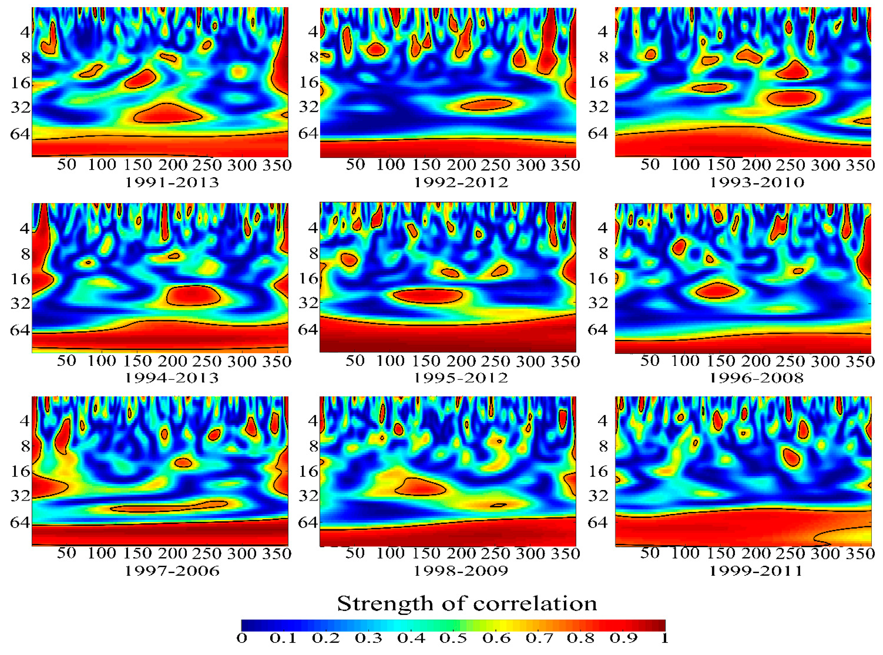
2.3.1. Wavelet Coherence

Wavelet coherence is a useful approach for determining the correlations and similarities of patterns in two time series at various scales. For two independent time series, n and m, the wavelet transform was defined as $W_t^n\left(s\right)$ and $W_t^m\left(s\right)$. Then the cross-wavelet spectrum of n and m time series was calculated as:

$$W_t^{nm}\left(s\right)=W_t^n\left(s\right)W_t^{m\ast }\left(s\right)$$

(2)

In Equation (2), * denoted the complex conjugate, t and s represented the time index and scale, respectively. The definition of wavelet coherence could be interpreted as the absolute value squared of the smoothed $W_t^{nm}\left(s\right)$ [34]:

$$R_t^2\left(s\right)=\frac{{\left|S\left(s^{-1}{W}_t^{nm}\left(s\right)\right)\right|}^2}{S\left(S^{-1}{\left|W_t^n\left(s\right)\right|}^2\right)\ast S\left(S^{-1}{\left|W_t^m\left(s\right)\right|}^2\right)}$$

(3)

where S was a smoothing operator. To determine the 95% significance level of the wavelet coherence results, the Monte Carlo method was implemented. More detailed descriptions and applications about the wavelet coherence could be found in [35,36]. A MATLAB software package for performing the wavelet coherence can be found at http://grinsted.github.io/wavelet-coherence/.

Two indices, including mean wavelet coherence (MWC) and percent area of significant coherence (PASC), were introduced to evaluate the performances of the wavelet coherence [37,38]. MWC and PASC denoted the mean value of the wavelet coherence and the proportion of significant coherence area to the whole wavelet domain, at all scales and periods, respectively. The larger MWC and PASC indicated that the patterns in two time series are more correlated in nature.

2.3.2. Cubist

In this study, Cubist was implemented to construct the predictive models between precipitation and a suite of land surface variables, including NDVI, LST and topographical indices. The Cubist algorithm has two main characteristics: partitioning and model building. By implementing the Cubist method, the entire dataset was divided into several subsets which were grouped according to their geographic similarities. For each separate subset, the rule-based model was constructed by applying a stepwise regression strategy. More details on the Cubist method can be found elsewhere, such as [15,16]. In this study, the Cubist model was generated using the package Cubist in R (https://cran.r-project.org/web/packages/Cubist/).

2.3.3. Mann–Kendall Trend Test

The sequential Mann–Kendall (SQ-MK) test was used in this study to determine the approximate start point of a significant trend [39,40]. Meanwhile, this test could also reflect the fluctuations in the trend [41,42]. The general trend and mutation time in a time series were estimated as follows.

For collected time-sequencing precipitation data $p_1,p_2,p_3,\dots ,p_t$, the time-ordered series ($S_n$) according to their collection sequence was given as follows:

$$S_n={\displaystyle \sum }_{i=1}^n{k}_i,\left(n=2,3,\dots ,t\right)$$

(4)

in which,

$$k_i=\{\begin{array}{c}+1,\hspace{1em}{p}_i>p_j\\ 0,\hspace{1em}{p}_i\le p_j\end{array},\left(j=1,2,3\dots ,i\right)$$

(5)

where $p_i$ and $p_j$ were the precipitation amounts at times $i$ and $j$, and the progressive statistic ($U{F}_{\left(S_n\right)}$) was defined as:

$$U{F}_{\left(S_n\right)}=\frac{\left[S_n-E\left(S_n\right)\right]}{\sqrt{Var\left(S_n\right)}},\left(n=2,3\dots ,t\right)$$

(6)

$E\left(S_n\right)$ and $Var\left(S_n\right)$ denoted the mean and variance of $S_n$, which were calculated as Equations (7) and (8), respectively.

$$E\left(S_n\right)=\frac{t\left(t+1\right)}{4}$$

(7)

$$Var\left(S_n\right)=\frac{t\left(t-10\right)\left(2t+5\right)}{72}$$

(8)

$U{F}_{\left(S_n\right)}$ was the forward sequence and all $U{F}_{\left(S_n\right)}$ would result in a curve (UF) which started at 0 (when n = 1). The similar analysis was then employed in the reverse data series. By applying this method, a retrograde $U{B}_{\left(S_n\right)}$ could be computed by:

$$\{\begin{array}{c}U{B}_{\left(S_n\right)}=-U{F}_{\left(S_{n^{\prime }}\right)}\\ n^{\prime }=t+1-n\end{array},\left(n^{\prime },n=1,2,3\dots ,t\right)$$

(9)

For all $U{B}_{\left(S_n\right)}$, a curve was designed as UB. $S_n$ could be considered as normal distribution under the null hypothesis. For this study the confidence interval was taken as $\pm 1.96\left(p=0.05\right)$, which indicated that if the absolute value of $UF$ was larger than 1.96, the trend was considered to be significant at the 95% confidence level. The negative $UF$reflected a decreasing trend while the positive value of $UF$ represented an increasing trend in the time series. The intersection of $UF$ and $UB$curves represented the approximate mutation time of the trend within the precipitation time series.

2.3.4. Calibration and Validation

As the DS are an indirect precipitation estimates in nature, the regional bias and random errors from the estimates should be evaluated and corrected [43]. Thus, a fraction of the rain gauges were chosen to calibrate the estimates while the remaining stations were used to independently evaluate the performance of the estimates (Figure 1). The gauges for calibration were selected according to their locations and recorded precipitation amounts. Four comparison indices were applied in the evaluation, including coefficients of determination (R²), bias, root mean square error (RMSE) and Nash–Sutcliffe efficiency (NSE).

$${\mathrm{R}}^2={\left(\frac{{{\displaystyle \sum }}_{i=1}^n\left(G_i-\overline{G}\right)\times \left(P_i-\overline{P}\right)}{\sqrt{{{\displaystyle \sum }}_{i=1}^n{\left(G_i-\overline{G}\right)}^2}\times \sqrt{{{\displaystyle \sum }}_{i=1}^n{\left(P_i-\overline{P}\right)}^2}}\right)}^2$$

(10)

$$\mathrm{bias}=\frac{{{\displaystyle \sum }}_{i=1}^n{P}_i}{{{\displaystyle \sum }}_{i=1}^n{G}_i}-1$$

(11)

$$\mathrm{RMSE}=\sqrt{\frac{{{\displaystyle \sum }}_{i=1}^n{\left(P_i-G_i\right)}^2}{n}}$$

(12)

$$\mathrm{NSE}=1-\frac{{{\displaystyle \sum }}_{i=1}^n{\left(P_i-G_i\right)}^2}{{{\displaystyle \sum }}_{i=1}^n{\left(G_i-\overline{G}\right)}^2}$$

(13)

$P_i$ was the precipitation estimate; $G_i$ and $\overline{G}$ were the annual and mean annual values based on ground observations, respectively; $i$ and n were the index and total number of comparison pairs, respectively.

The R² reflects the strength of the liner relationship between the precipitation estimates and ground observations, ranging between 0 and 1 with an optimal value of 1. The bias measures the tendency of the estimates to be overestimated (positive values) or underestimated (negative values), with a perfect value of 0. The RMSE indicates the magnitude of error estimations, the smaller RMSE means more reliable estimates compared to ground observations. The NSE [44], which varies from −$\infty$ to 1, measures the magnitude of the variance of the residuals compared to those of the observed values of precipitation, and the perfect value of NSE is 1 while being negative indicates poor precipitation estimations.

2.3.5. Main Steps to Retrospectively Obtain Precipitation Estimates (~1 km) in the 1990s

The main steps were described as follows:

(1)

Wavelet coherence was firstly applied to detect the inherent similarities and correlations of precipitation between the target time periods, from 1990 to 1999, and reference time periods, from 2000 to 2013, at different temporal scales based on ground observations (Figure 2). The target year and the corresponding reference year were determined when the MWC and PASC values were largest.

(2)

All land surface characteristics, including annual mean LST data, annual mean NDVI and topographical parameters, were aggregated to 0.25$°$ from corresponding data at their original spatial resolutions, from 2000 to 2013. Then, the Cubist models were built between TMPA data and land surface variables in the reference years at a spatial resolution of 0.25$°$.

(3)

In the target years from 1990 to 1999, the land surface variables at ~1 km were firstly obtained. In terms of NDVI, we interpolated the GIMMS NDVI (1/12°) into those at ~1 km using simple spline tension interpolator, which was typically suitable for regularly-spaced data [7], in this study. The gridded GIMMS NDVI data had been converted into those in point-based format, before the interpolations were conducted in ArcGIS 10.2 software (https://www.esri.com/en-us/home). The DS were obtained by applying the Cubist models generated in step (2), in the corresponding reference years determined in step (1), on the land surface variables in the target years (Figure 2).

(4)

The calibration data was used to correct the DS, in the target years, obtained in step (3). At the beginning, the point-based ratios, by comparing the ground observations to DS, were interpolated into gridded estimates (~1 km) using the ordinary kriging technique [13]. Moreover, the final DS with gauge calibrations were obtained by multiplying the gridded ratios by the DS without gauge calibration obtained in step (3).

(5)

The performances of DS at ~1 km resolution were assessed through validation stations. Meanwhile, the performance of CHIRPS was also evaluated through the same validation stations and compared with those of the DS with/without gauge calibration (Figure 2).

3. Results

3.1. The Trends and Mutation of Precipitation over the Tibetan Plateau (TP)

Figure 3 presented the statistical curves of the $UF$ and $UB$, using the SQ–MK test based on ground observations from rain gauges, in the period from 1954 to 2013 over the TP. The $UF$ and $UB$ curves were intersected in 1984, moreover, the intersection was inside the confidence interval, which indicated that the precipitation patterns over the TP were changed in 1984. The $UF$ curve represented the general trend of the precipitation. According to the $UF$ curve, the temporal variations in precipitation over the TP from 1954 to 2013 could be approximately divided into three periods. The variations in precipitation fluctuated in the first period between 1954 and the late 1960s. The second period was between 1970 and the early 1980s, in which the precipitation variations exhibited a decreasing trend. In the third period (after 1984), the precipitation variations showed a steep increasing trend, and the increasing trend was considered to be significant since 1990, because the $UF$ curve exceeded the line of 95% confidence level. Therefore, this study focused on the period from 1990 to 1999, with the significant increasing trend of precipitation over the TP.

3.2. Inter-Annual Correlations and Similarities of Precipitation Patterns

The correlations and similarities of precipitation patterns in the target year, 1990, and reference years from 2000 to 2013, were shown in Figure 4. According to the general trend of the variability, the temporal scales were divided into four groups: very short-period (<8 days), short-period (8–32 days), medium-period (32–64 days) and long-period (>64 days). At the very short-period and short-period temporal scales, the correlations of precipitation patterns in the target year and those in the reference years were not strong, although several significant correlations were observed in some discrete time. In the medium-period scale, the precipitation patterns in 1990 and those in 2006 showed significant correlations from the mid to the end of the year. Furthermore, the statistical correlations of precipitation patterns, in 1990 and those in 2006, were much more significant at the long period scale than those at the medium-period scale (Figure 4). Thus, the precipitation patterns in the reference year, 2006, was considered as the optimal reference to stand for those in 1990.

The quantitative evaluations of the correlations of precipitation patterns in the target year, 1990, and reference years from 2000 to 2013, at different temporal scales, were displayed in

Table 1. Statistical results of wavelet coherence based on correlations and similarities of precipitation patterns in the target year, 1990, and reference years from 2000 to 2013.

	Mean Wavelet Coherence (MWC)					Percent Area of Significant Coherence (PASC) (%)
	Temporal Scales					Temporal Scales
	<8 day	8–32 day	32–64 day	>64 day	All Scales	<8 day	8–32 day	32–64 day	>64 day	All Scales
1990–2000	0.34	0.41	0.42	0.53	0.42	12.07	18.40	16.71	5.55	14.93
1990–2001	0.31	0.33	0.29	0.42	0.34	8.80	8.12	5.98	5.33	7.60
1990–2002	0.29	0.33	0.22	0.36	0.30	7.01	4.68	1.32	0.00	4.10
1990–2003	0.28	0.27	0.32	0.64	0.37	7.17	1.49	9.19	20.21	11.05
1990–2004	0.24	0.22	0.42	0.31	0.30	3.63	1.12	17.58	1.47	4.85
1990–2005	0.28	0.28	0.38	0.43	0.34	7.46	3.22	2.22	0.00	3.91
1990–2006	0.34	0.39	0.53	0.70	0.49	10.00	15.89	36.22	40.00	27.02
1990–2007	0.38	0.36	0.43	0.51	0.42	15.58	7.36	9.26	4.66	10.63
1990–2008	0.33	0.32	0.32	0.31	0.32	8.88	7.91	8.54	0.00	7.10
1990–2009	0.34	0.34	0.29	0.46	0.36	8.38	6.79	3.88	4.94	7.44
1990–2010	0.31	0.32	0.42	0.21	0.31	5.45	8.63	12.55	0.00	6.81
1990–2011	0.38	0.34	0.35	0.41	0.37	14.58	8.31	1.49	0.00	7.65
1990–2012	0.34	0.33	0.46	0.52	0.41	10.58	11.49	25.00	4.61	12.75
1990–2013	0.32	0.39	0.38	0.32	0.35	8.98	12.75	13.97	0.00	9.57

.The largest values of MWC (~0.70) and PASC (~40.00%) were determined in the results, based on the correlations of precipitation patterns in 1990 and those in 2006, at a long period (>64 days), which coincided with the wavelet coherence results displayed in Figure 4. The strength of the correlations of precipitation patterns in 1990 and 2006 outperformed than those in other reference years, considering the largest mean values of MWC (0.49) and PASC (27.02%).

Figure 5a displayed the curves of the precipitation variations in 1990 (blue line) and those in 2006 (red line), based on the mean values of ground observations over the TP. The precipitation patterns in two years showed similar characteristics and trends throughout the entire year, such as the alternations of dry and wet seasons, and the precipitation peaks, and valleys in specific periods. The relative differences in precipitation between 1990 and 2006 were displayed in Figure 5b. Generally, the differences were almost randomly distributed, at daily scale, year-round, which indicated the precipitation differences did not have any specific patterns. Therefore, wavelet coherence method could determine the inherent similarities between two precipitation patterns in target years and those in reference years, and reveal strong correlations.

Hereafter, the correlations and similarities of precipitation patterns in each target year, from 1991 to 1999, and the corresponding reference year, from 2000 to 2013, were matched. The wavelet coherence results based on the correlations of precipitation patterns in the target years from 1991 to 1999 and its corresponding reference years were shown in Figure 6. Similar to the situation in 1990, there were also limited correlations of precipitation patterns detected in discrete period at a very short period scale (<8 day) and short period scale (8–16 day), respectively. However, the strong correlations were always determined at long period temporal scale (>64 days), indicating the precipitation patterns in two independent years were correlated well at the bi-monthly scale.

Table 2. Statistical results of wavelet coherence based on correlations and similarities of precipitation patterns in the target years, from 1991 to 1999, and reference years from 2000 to 2013.

	MWC					PASC (%)
	Temporal Scales					Temporal Scales
	<8 day	8–32 day	32–64 day	>64 day	All Scales	<8 day	8–32 day	32–64 day	>64 day	All Scales
1991–2013	0.31	0.38	0.47	0.79	0.48	7.93	11.27	17.53	42.52	23.49
1992–2012	0.42	0.29	0.18	0.79	0.42	19.66	10.34	0.20	38.68	23.14
1993–2010	0.29	0.35	0.44	0.82	0.47	6.91	13.90	16.28	43.66	20.19
1994–2013	0.34	0.35	0.41	0.83	0.48	11.91	14.57	18.28	39.47	25.02
1995–2012	0.33	0.35	0.52	0.96	0.54	9.23	14.29	31.13	50.00	29.43
1996–2008	0.34	0.32	0.25	0.81	0.43	10.82	8.38	0.82	39.16	19.58
1997–2006	0.34	0.38	0.39	0.88	0.50	10.64	12.77	16.61	44.73	25.30
1998–2009	0.32	0.36	0.37	0.89	0.48	7.31	8.53	12.38	45.61	22.37
1999–2011	0.34	0.40	0.66	0.80	0.55	11.06	21.06	34.53	43.69	27.58

displayed the quantitative evaluations of the correlations of precipitation patterns in the target years, from 1991 to 1999, and the reference years from 2000 to 2013, at different temporal scales. In accordance with the wavelet coherence results presented in Figure 6, the strongest correlations of precipitation patterns in the target years and the corresponding reference years were detected at long period (>64 day). Additionally, the values of MWC and PASC at long period temporal scale (>64 day) were larger than those at shorter temporal scales, in terms of MWC values (>0.79) and PASC values (>39.16%). Generally speaking, the mean values of MWC and PASC, at all scales, were larger than 0.42 and 19.58%, respectively.

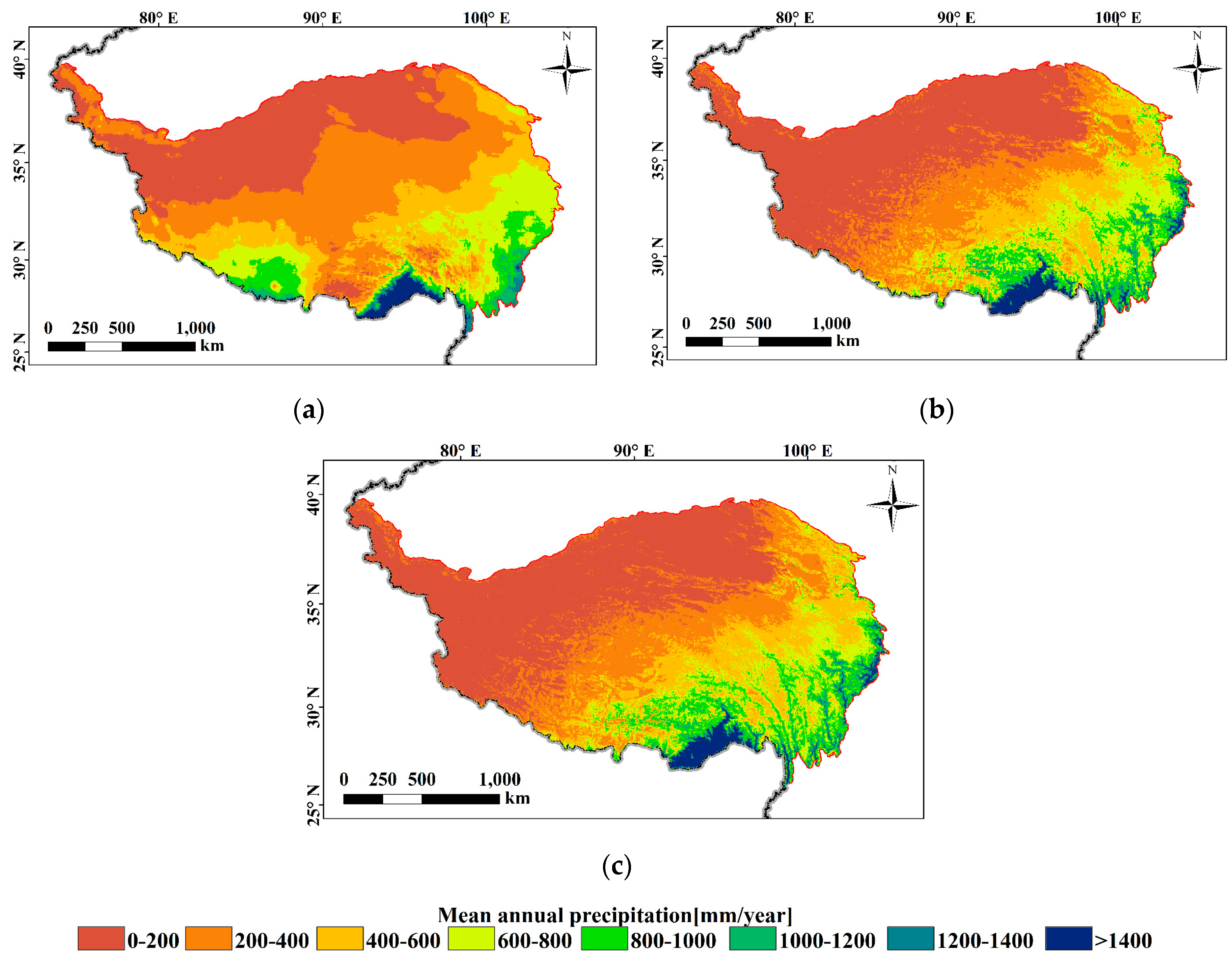
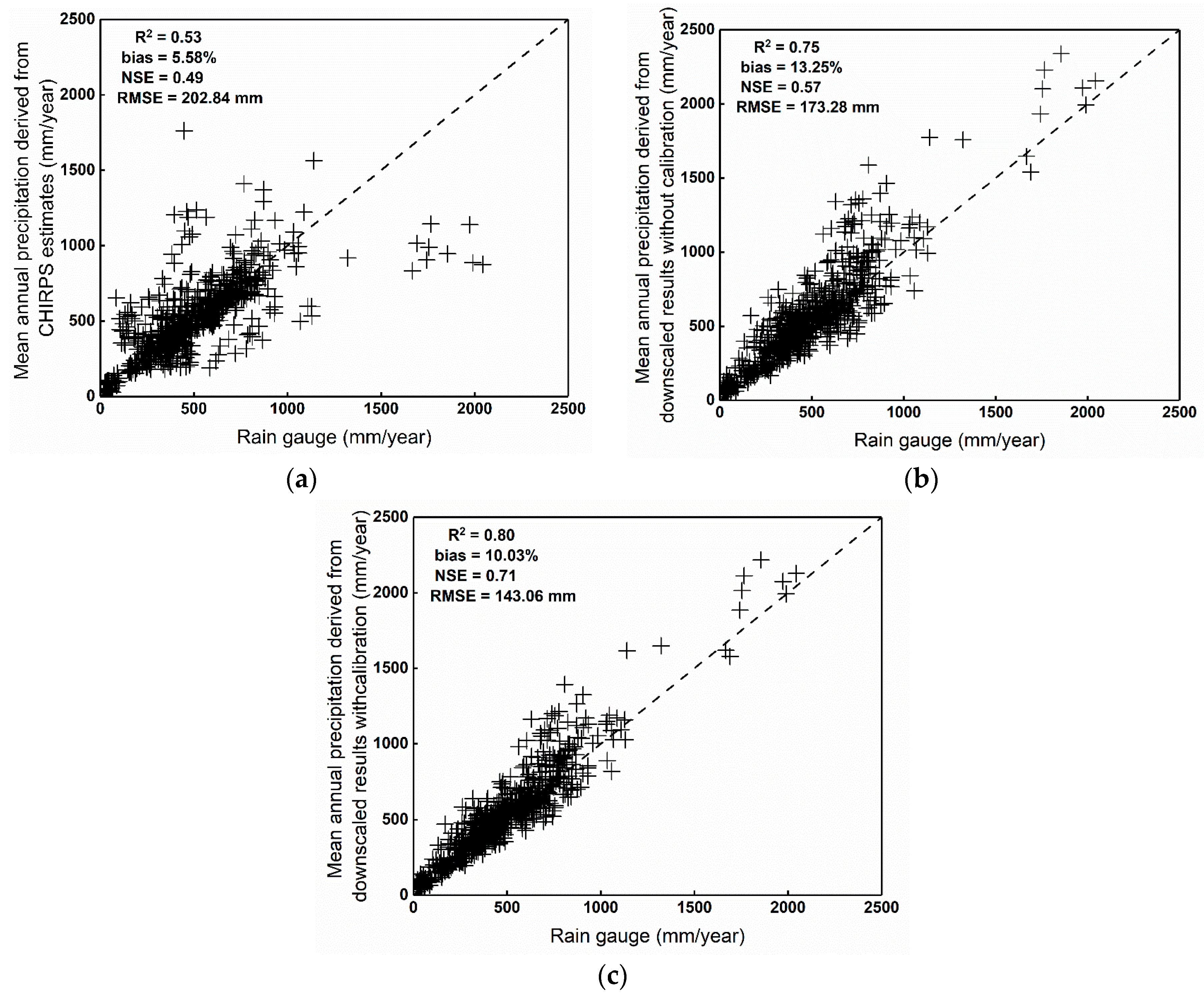
3.3. Retrospectively Downscaled Results and Validations

Based on wavelet coherence and the Cubist algorithm, we retrospectively obtained the DS over the TP for the period from 1990 to 1999, at ~1 km resolution. In addition, CHIRPS data from 1990 to 1999 was also introduced and evaluated, in order to compare the performances with those of DS. The spatial pattern of CHIRPS data, determined by averaging precipitation estimates in the years from 1990 to 1999, was shown in Figure 7a, while the spatial patterns of the DS without gauge calibration and those with gauge calibration were shown in Figure 7b,c, respectively. Both CHIRPS data and the DS data showed a similar trend of precipitation over the TP. However, it was obvious that CHIRPS data presented relatively larger precipitation estimates in a small part of the south-western TP with annual precipitation around 800–1000 mm/year, while the annual precipitation of the DS was under 600 mm/year. Due to the coarse resolution of CHIRPS data (~5 km), the spatial pattern of CHIRPS demonstrated significant spatial divisions. The spatial trends of DS varied gradually from south-east to north-west, over the TP, because of the finer spatial resolution (~1 km).

To compare the performances of the DS, both without and with rain gauge calibration, with those of CHIRPS data, we validated these precipitation products against ground observations for the period from 1990 to 1999. The validation of CHIRPS data was shown in Figure 8a, while Figure 8b,c displayed the validations of the DS without rain gauge calibration and those with rain gauge calibration, respectively. Generally speaking, CHIRPS data had the worst performance (R² ~ 0.53, bias ~ 5.58%, NSE ~ 0.49 and RMSE ~ 202.84 mm) among the three precipitation products. The DS without gauge calibration outperformed CHIRPS data, with larger correlations and lower errors (R² ~ 0.75, NSE ~ 0.57, and RMSE ~ 173.28 mm). The DS with gauge calibration improved the accuracy (R² ~ 0.80, bias ~ 10.03%, NSE ~ 0.71 and RMSE ~ 143.06 mm), compared to those without gauge calibration.

Table 3. Statistical results of the CHIRPS data, the DS without and with gauge calibration, against ground observations in the years from 1990 to 1999.

		1990	1991	1992	1993	1994	1995	1996	1997	1998	1999
CHIRPS	R2	0.42	0.49	0.49	0.53	0.50	0.62	0.41	0.56	0.61	0.58
	Bias (%)	5.65	5.96	4.19	5.72	2.81	3.30	4.20	3.65	7.62	4.29
	Nash–Sutcliffe efficiency (NSE)	0.26	0.48	0.49	0.52	0.48	0.62	0.35	0.59	0.55	0.41
	Root mean square error (RMSE) (mm)	255.12	214.09	202.13	213.36	181.41	185.11	212.75	162.42	207.95	186.39
DS without calibration	R2	0.77	0.72	0.79	0.73	0.78	0.70	0.72	0.74	0.75	0.71
	Bias (%)	19.05	18.39	15.58	14.59	15.89	15.63	10.33	12.16	18.87	10.73
	NSE	0.63	0.56	0.75	0.74	0.74	0.60	0.69	0.72	0.49	0.65
	RMSE (mm)	180.34	195.74	141.00	157.26	141.66	191.28	147.98	146.49	222.87	148.43
DS with calibration	R2	0.83	0.79	0.84	0.81	0.85	0.79	0.80	0.83	0.84	0.79
	Bias (%)	14.29	13.79	11.69	10.94	5.41	11.72	7.74	1.62	14.15	8.05
	NSE	0.79	0.75	0.86	0.85	0.79	0.77	0.82	0.80	0.71	0.80
	RMSE (mm)	135.26	146.81	115.75	117.95	114.39	143.47	110.99	119.87	167.16	111.33

displays the validation results of CHIRPS data, the DS both with and without rain gauge calibration, against ground observations, in the years from 1990 to 1999, over the TP. The CHIRPS data performed relatively worse, with smaller correlations and larger errors (R² varying from 0.41 to 0.62, NSE ranging from 0.26 to 0.62, and RMSE fluctuating between 162.42 mm and 255.12 mm). Compared with CHIRPS data, the DS without gauge calibration showed better performances (R² > 0.70, NSE > 0.49). The accuracy of the DS with gauge calibration outperformed CHIRPS and DS without gauge calibration in the years from 1990 to 1999 (R² ~ 0.80, NSE ~ 0.80, and RMSE ~ 120 mm).

Figure 9a displayed the spatial distributions of mean annual precipitation obtained from CHIRPS, DS without gauge calibration and DS with gauge calibration, while Figure 9b–e demonstrated spatial distributions of R², bias, RMSE and NSE, respectively, of CHIRPS data, the DS without gauge calibration and DS with gauge calibration, against ground observations, from 1990 to 1999. Generally, the spatial distributions of annual precipitation at the stations over the TP were captured well by CHIRPS, DS both without and with gauge calibration. In terms of the evaluation indices, all the precipitation products showed better agreements to ground observations in the southern and eastern TP where precipitation was relatively larger, but had poor performances in western and northern TP, where precipitation was relatively smaller. The DS with gauge calibration showed the best performance considering the strong correlations between precipitation estimates and ground observations with R² values even >0.8 in most sites, while the R² values of CHIRPS data were acceptable (R² > 0.6) in the south-eastern TP, but decreased significantly in the north and south-western parts (R² ~ 0.2). The bias and RMSE values of the DS with calibration also declined, especially over regions close to the Himalayan Mountains, compared with those of CHIRPS data. The NSE values of DS with gauge calibration also improved. These results demonstrated that the DS with gauge calibration provided more reliable precipitation estimates than CHIRPS data and DS without gauge calibration, over the TP.

3.4. Comparisons of Precipitation Estimates at Specific Stations

Based on the evaluation results presented in Figure 9, we found that precipitation estimates based on CHIRPS and DS had significant differences over TP, for example, in region A and region B, which could be found in Figure 1. There were four validation stations located in region A, namely Gaize, Pulan, Lazi and Nielaer, with elevation >3800 m above sea level. The mean annual precipitation were 156.5 mm/year, 131.4 mm/year, 362.1 mm/year and 551.8 mm/year, at Gaize, Pulan, Lazi and Nielaer stations, respectively, in region A. Another four validation stations, including Xiaozaohuo, Delingha, GeErMu and NuoMuHong, were distributed in region B. By contrast to region A, which is a mountainous area, region B is a basin area with elevation ~2800 m. The mean annual precipitation recorded by Xiaozaohuo, Delingha, GeErMu and NuoMuHong were 29.2 mm/year, 173.0 mm/year, 51.8 mm/year and 43.3 mm/year, respectively.

Figure 10 illustrates the comparisons of annul precipitation at the aforementioned eight stations based on ground observations, and precipitation estimates obtained from CHIRPS and the DS. The precipitation at the four stations, located in region A were poorly captured by CHIRPS data. It could be seen that CHIRPS data tended to greatly overestimate precipitation at each station in region A, which suggested that CHIRPS data could not capture the annual precipitation volumes appropriately, and provided unfavorable precipitation information in region A. The precipitation estimates obtained from DS were in better agreement with ground observations at the Gaize and Nielaer stations, compared with those of CHIRPS data. While in region B, both the CHIRPS and the DS had reasonable performances at Delingha station, however, CHIRPS data highly overestimated precipitation volumes in 1996 and 1997. Additionally, the DS captured annual precipitation well at Delingha station, such as the precipitation peak in 1992 and 1998, which indicated the better accuracy of the DS. Overall, the DS outperformed CHIRPS data in regions A and B at the specific stations.

4. Discussion

4.1. Improvements and Limations of the Framework

In this study, we tried to obtain precipitation estimates (~1 km) from 1990 to 1999 over the TP retrospectively. The precipitation estimates, obtained by the proposed framework, had reasonable performances compared with those of CHIRPS data, against ground observations. Wavelet coherence demonstrated its abilities to reveal the correlations and similarities of precipitation patterns in two independent years. Meanwhile, Cubist is a newly capable spatial data mining algorithm used to downscale coarse satellite-based precipitation data [14,15]. The Cubist algorithm considered the non-stationary relationships between precipitation and land surface variables. Meanwhile, Cubist also performed robustly when considering a large number of predictor variables. Additionally, the liner models generated by Cubist were interpretable [14], while other machine learning algorithms, such as random forest and artificial neutral networks, do not have this ability. Therefore, this methodological framework, combining wavelet coherence and Cubist, had great potentials in obtaining precipitation estimates for the period, in 1990s, when TMPA data is inaccessible.

However, the accuracy of the DS generated by this framework was also subjected to several error sources. Firstly, the correlations and similarities of precipitation patterns between the target years, from 1990 to 1999, and the optimal reference years, from 2000 to 2013, were determined. But the period of the reference years may be not long enough to detect the ‘best’ year, in which the TMPA and Cubist models were applied retrospectively to obtain the DS. For example, the precipitation patterns in 2006 were selected as the reference to obtain precipitation estimates for the target years both in 1990 and 1997. Additionally, to obtain precipitation estimates at ~1 km resolution, land surface variables with both finer resolutions (~1 km) and better accuracy were also needed in 1990s. For example, there were limited NDVI and LST datasets extending to the 1990s. In this study, GIMMS NDVI 3g data with a spatial resolution of 1/12°, were interpolated to obtain the ~1 km NDVI data, which may result in unavoidable uncertainties in the DS. Besides, the selection of calibration data may also influence the accuracy of the precipitation estimates [45,46].

4.2. Possible Applications of the Retrospectively Downscaled Results in Related Fields

Long-term precipitation estimates with both finer spatial resolutions (~1 km) and better accuracy are urgently needed in various related fields, such as soil science, ecology and water balance research [47,48,49,50]. The DS obtained in this study could be used in predicting soil properties, like soil organic carbon [47,48], which was abundantly stored in the permafrost in TP and was sensitive to climate change. Although the TP provides water resources supporting enormous ecosystems in China and South-east Asia and >1.4 billion people downstream [49], and different climate change patterns were significantly detected by previous research, long-term precipitation estimates with both finer spatial resolutions and better accuracy are still needed [51], for example, in investigating the variation patterns of precipitation and glaciers.

5. Conclusions

In this study, a new methodological framework, combining wavelet coherence and Cubist, was proposed to obtain retrospectively the DS from 1990 to 1999 over the TP. Meanwhile, a calibration procedure was also incorporated. The performance of the DS was evaluated using ground observations. The major findings of this study were as follows: (1) the mutation in precipitation patterns was detected in 1984, over the TP, and a significant increasing trend in precipitation was found after 1990; (2) the DS with gauge calibration showed continuous trends over the TP from south-east to north-west; (3) the DS with gauge calibration were in better agreement with ground observations compared with those of CHIRPS data. Therefore, the methodological framework developed in this study could serve as an alternative approach to obtain downscaled results in 1990s retrospectively.

References

1. Muller, C.J.; O’Gorman, P.A. An energetic perspective on the regional response of precipitation to climate change. Nat. Clim. Chang. 2011, 1, 266–271. [Google Scholar] [CrossRef]
2. Qiu, J. China: The third pole. Nat. News 2008, 454, 393–396. [Google Scholar] [CrossRef] [Green Version]
3. Liu, X.; Chen, B. Climatic warming in the Tibetan Plateau during recent decades. Int. J. Climatol. 2000, 20, 1729–1742. [Google Scholar] [CrossRef] [Green Version]
4. Zhang, D.; Huang, J.; Guan, X.; Chen, B.; Zhang, L. Long-term trends of precipitable water and precipitation over the Tibetan Plateau derived from satellite and surface measurements. J. Quant. Spectrosc. Radiat. Transf. 2013, 122, 64–71. [Google Scholar] [CrossRef]
5. Ma, Y.; Tang, G.; Long, D.; Yong, B.; Zhong, L.; Wan, W.; Hong, Y. Similarity and error intercomparison of the GPM and its predecessor-TRMM multisatellite precipitation analysis using the best available hourly gauge network over the Tibetan Plateau. Remote Sens. 2016, 8, 569. [Google Scholar] [CrossRef]
6. Kyriakidis, P.C.; Kim, J.; Miller, N.L. Geostatistical mapping of precipitation from rain gauge data using atmospheric and terrain characteristics. J. Appl. Meteorol. 2001, 40, 1855–1877. [Google Scholar] [CrossRef]
7. Ma, Z.; Tan, X.; Yang, Y.; Chen, X.; Kan, G.; Ji, X.; Lu, H.; Long, J.; Cui, Y.; Hong, Y. The First Comparisons of IMERG and the Downscaled Results Based on IMERG in Hydrological Utility over the Ganjiang River Basin. Water 2018, 10, 1392. [Google Scholar] [CrossRef]
8. Immerzeel, W.W.; Rutten, M.M.; Droogers, P. Spatial downscaling of TRMM precipitation using vegetative response on the Iberian Peninsula. Remote Sens. Environ. 2009, 113, 362–370. [Google Scholar] [CrossRef]
9. Teng, H.; Shi, Z.; Ma, Z.; Li, Y. Estimating spatially downscaled rainfall by regression kriging using TRMM precipitation and elevation in Zhejiang Province, southeast China. Int. J. Remote Sens. 2014, 35, 7775–7794. [Google Scholar] [CrossRef]
10. Jia, S.; Zhu, W.; Lű, A.; Yan, T. A statistical spatial downscaling algorithm of TRMM precipitation based on NDVI and DEM in the Qaidam Basin of China. Remote Sens. Environ. 2011, 115, 3069–3079. [Google Scholar] [CrossRef] [Green Version]
11. Xu, S.; Wu, C.; Wang, L.; Gonsamo, A.; Shen, Y.; Niu, Z. A new satellite-based monthly precipitation downscaling algorithm with non-stationary relationship between precipitation and land surface characteristics. Remote Sens. Environ. 2015, 162, 119–140. [Google Scholar] [CrossRef]
12. Chen, F.R.; Liu, Y.; Liu, Q.; Li, X. Spatial downscaling of TRMM 3B43 precipitation considering spatial heterogeneity. Int. J. Remote Sens. 2015, 35, 3074–3093. [Google Scholar] [CrossRef]
13. Fang, J.; Du, J.; Xu, W.; Shi, P.J.; Li, M.; Ming, X.D. Spatial downscaling of TRMM precipitation data based on the orographical effect and meteorological conditions in a mountainous area. Adv. Water Resour. 2013, 61, 42–50. [Google Scholar] [CrossRef]
14. Shi, Y.; Song, L. Spatial Downscaling of Monthly TRMM Precipitation Based on EVI and Other Geospatial Variables Over the Tibetan Plateau From 2001 to 2012. Mt. Res. Dev. 2015, 35, 180–194. [Google Scholar] [CrossRef]
15. Ma, Z.; Shi, Z.; Zhou, Y.; Xu, J.; Yu, W.; Yang, Y. A spatial data mining algorithm for downscaling TMPA 3B43 V7 data over the Qinghai–Tibet Plateau with the effects of systematic anomalies removed. Remote Sens. Environ. 2017, 200, 378–395. [Google Scholar] [CrossRef]
16. Ma, Z.; Zhou, Y.; Hu, B.; Liang, Z.; Shi, Z. Downscaling annual precipitation with TMPA and land surface characteristics in China. Int. J. Climatol. 2017, 37, 5107–5119. [Google Scholar] [CrossRef]
17. Vachaud, G.; De Silans, A.P.; Balabanis, P.; Vauclin, M. Temporal stability of spatially measured soil water probability density function. Soil Sci. Soc. Am. J. 1985, 49, 822–828. [Google Scholar] [CrossRef]
18. Biswas, A.; Si, B.C. Scales and locations of time stability of soil water storage in a hummocky landscape. J. Hydrol. 2011, 408, 100–112. [Google Scholar] [CrossRef]
19. Sang, Y.F. A review on the applications of wavelet transform in hydrology time series analysis. Atmos. Res. 2013, 122, 8–15. [Google Scholar] [CrossRef]
20. Zhisheng, A.; Kutzbach, J.E.; Prell, W.L.; Porter, S.C. Evolution of Asian monsoons and phased uplift of the Himalaya Tibetan plateau since Late Miocene times. Nature 2001, 411, 62–66. [Google Scholar] [CrossRef]
21. Yao, T.; Thompson, L.; Yang, W.; Yu, W.; Gao, Y.; Guo, X.; Yang, X.; Duan, K.; Zhao, H.; Xu, B.; et al. Different glacier status with atmospheric circulations in Tibetan Plateau and surroundings. Nat. Clim. Chang. 2012, 2, 663–667. [Google Scholar] [CrossRef]
22. Huffman, G.J.; Bolvin, D.T.; Nelkin, E.J.; Wolff, D.B.; Adler, R.F.; Gu, G.; Hong, Y.; Bowman, K.P.; Stocker, E.F. The TRMM multisatellite precipitation analysis (TMPA): Quasi-global, multiyear, combined-sensor precipitation estimates at fine scales. J. Hydrometeorol. 2007, 8, 38–55. [Google Scholar] [CrossRef]
23. Funk, C.C.; Peterson, P.J.; Landsfeld, M.F.; Pedreros, D.H.; Verdin, J.P.; Rowland, J.D.; Romero, B.E.; Husak, G.J.; Michaelsen, J.C.; Verdin, A.P. A Quasi-Global Precipitation Time Series for Drought Monitoring. U.S. Geol. Surv. Data Ser. 2014, 832, 4. [Google Scholar]
24. Funk, C.; Peterson, P.; Landsfeld, M.; Pedreros, D.; Verdin, J.; Shukla, S.; Husak, G.; Rowland, J.; Harrison, L.; Hoell, A. The climate hazards infrared precipitation with stations—A new environmental record for monitoring extremes. Sci. Data 2015, 2, 150066. [Google Scholar] [CrossRef]
25. Xiao, J.; Moody, A. Trends in vegetation activity and their climatic correlates: China 1982 to 1998. Int. J. Remote Sens. 2004, 25, 5669–5689. [Google Scholar] [CrossRef]
26. Evans, K.L.; James, N.A.; Gaston, K.J. Abundance, species richness and energy availability in the North American avifauna. Glob. Ecol. Biogeogr. 2006, 15, 372–385. [Google Scholar] [CrossRef]
27. Grist, J.; Nicholson, S.E.; Mpolokang, A. On the use of NDVI for estimating rainfall fields in the Kalahari of Botswana. J. Arid Environ. 1997, 35, 195–214. [Google Scholar] [CrossRef]
28. Iwasaki, H. NDVI prediction over Mongolian grassland using GSMaP precipitation data and JRA-25/JCDAS temperature data. J. Arid Environ. 2009, 73, 557–562. [Google Scholar] [CrossRef]
29. Sobrino, J.A.; Raissouni, N. Toward remote sensing methods for land cover dynamic monitoring: Application to Morocco. Int. J. Remote Sens. 2000, 21, 353–366. [Google Scholar] [CrossRef]
30. Sobrino, J.A.; Li, Z.L.; Stoll, M.P.; Becker, F. Improvements in the split-window technique for land surface temperature determination. IEEE Trans. Geosci. Remote Sens. 1994, 32, 243–253. [Google Scholar] [CrossRef]
31. Coll, C.; Caselles, V. A split-window algorithm for land surface temperature from advanced very high resolution radiometer data: Validation and algorithm comparison. J. Geophys. Res. Atmospheres 1997, 102, 16697–16713. [Google Scholar] [CrossRef] [Green Version]
32. Atitar, M.; Sobrino, J.A. A split-window algorithm for estimating LST from Meteosat 9 data: Test and comparison with in situ data and MODIS LSTs. IEEE Geosci. Remote Sens. Lett. 2009, 6, 122–126. [Google Scholar] [CrossRef]
33. Julien, Y.; Sobrino, J.A. Correcting AVHRR long term data record V3 estimated LST from orbital drift effects. Remote Sens. Environ. 2012, 123, 207–219. [Google Scholar] [CrossRef]
34. Torrence, C.; Webster, P.J. Interdecadal changes in the ENSO–monsoon system. J. Clim. 1999, 12, 2679–2690. [Google Scholar] [CrossRef]
35. Torrence, C.; Compo, G.P. A practical guide to wavelet analysis. Bull. Am. Meteorol. Soc. 1998, 79, 61–78. [Google Scholar] [CrossRef]
36. Grinsted, A.; Moore, J.C.; Jevrejeva, S. Application of the cross wavelet transform and wavelet coherence to geophysical time series. Nonlinear Process. Geophys. 2004, 11, 561–566. [Google Scholar] [CrossRef] [Green Version]
37. Hu, W.; Si, B.C.; Biswas, A.; Chau, H.W. Temporally stable patterns but seasonal dependent controls of soil water content: Evidence from wavelet analyses. Hydrol. Process. 2017, 31, 3697–3707. [Google Scholar] [CrossRef]
38. Zhao, R.; Biswas, A.; Zhou, Y.; Zhou, Y.; Shi, Z.; Li, H. Identifying localized and scale-specific multivariate controls of soil organic matter variations using multiple wavelet coherence. Sci. Total Environ. 2018, 643, 548–558. [Google Scholar] [CrossRef]
39. Sneyers, R. On the Statistical Analysis of Series of Observations; WMO Technical Note, No. 415; WMO: Geneva, Switzerland, 1990. [Google Scholar]
40. Matyasovszky, I. Detecting abrupt climate changes on different time scales. Theor. Appl. Climatol. 2011, 105, 445–454. [Google Scholar] [CrossRef]
41. Pingale, S.M.; Khare, D.; Jat, M.K.; Adamowski, J. Spatial and temporal trends of mean and extreme rainfall and temperature for the 33 urban centers of the arid and semi-arid state of Rajasthan, India. Atmos. Res. 2014, 138, 73–90. [Google Scholar] [CrossRef]
42. Nalley, D.; Adamowski, J.; Khalil, B.; Ozga-Zielinski, B. Trend detection in surface air temperature in Ontario and Quebec, Canada during 1967–2006 using the discrete wavelet transform. Atmos. Res. 2013, 132–133, 375–398. [Google Scholar] [CrossRef]
43. Tian, Y.; Huffman, G.J.; Adler, R.F.; Tang, L.; Sapiano, M.; Maggioni, V.; Wu, H. Modeling errors in daily precipitation measurements: Additive or multiplicative? Geophys. Res. Lett. 2013, 40, 2060–2065. [Google Scholar] [CrossRef] [Green Version]
44. Nash, J.E.; Sutcliffe, J.V. River flow forecasting through conceptual models part I—A discussion of principles. J. Hydrol. 1970, 10, 282–290. [Google Scholar] [CrossRef]
45. Ma, Z.Q.; Zhou, L.Q.; Yu, W.; Yang, Y.Y.; Teng, H.F.; Shi, Z. Improving TMPA 3B43 V7 Data Sets Using Land-Surface Characteristics and Ground Observations on the Qinghai–Tibet Plateau. IEEE Geosci. Remote Sens. Lett. 2018, 99, 1–5. [Google Scholar] [CrossRef]
46. Duan, Z.; Bastiaanssen, W.G.M. First results from version 7 TRMM 3B43 precipitation product in combination with a new downscaling-calibration procedure. Remote Sens. Environ 2013, 131, 1–13. [Google Scholar] [CrossRef]
47. Sanchez, P.A.; Ahamed, S.; Carré, F.; Hartemink, A.E.; Hempel, J.; Huising, J.; Lagacherie, P.; McBratney, A.B.; McKenzie, N.J.; de Lourdes, M.; et al. Digital soil map of the world. Science 2009, 325, 680–681. [Google Scholar] [CrossRef]
48. Klopfenstein, S.T.; Hirmas, D.R.; Johnson, W.C. Relationships between soil organic carbon and precipitation along a climosequence in loess-derived soils of the Central Great Plains, USA. Catena 2015, 133, 25–34. [Google Scholar] [CrossRef]
49. Immerzeel, W.W.; Van Beek, L.P.; Bierkens, M.F. Climate change will affect the Asian water towers. Science 2010, 328, 1382–1385. [Google Scholar] [CrossRef]
50. Wang, Y.Y.; Zhang, Y.Q.; Chiew, F.H.S.; McVicar, T.R.; Zhang, L.; Li, H.X.; Qin, G.H. Contrasting runoff trends between dry and wet parts of eastern Tibetan Plateau. Nat. Sci. Rep. 2017, 7, 1–7. [Google Scholar] [CrossRef]
51. Ma, Z.; Xu, Y.; Peng, J.; Chen, Q.; Wan, D.; He, K.; Shi, Z.; Li, H. Spatial and temporal precipitation patterns characterized by TRMM TMPA over the Qinghai-Tibetan plateau and surroundings. Int. J. Remote Sens. 2018, 39, 3891–3907. [Google Scholar] [CrossRef]
Figure 1. Distributions of rain gauges for validation and calibration over the Tibetan Plateau (TP).
Remotesensing 10 01974 g001
Figure 2. Flow chart for obtaining retrospective precipitation estimates at ~1 km, in 1990s, using wavelet coherence and Cubist.
Remotesensing 10 01974 g002
Figure 3. Mann–Kendall test of mean annual precipitation based on rain gauges over the TP from 1954 to 2013.
Remotesensing 10 01974 g003
Figure 4. The correlations and similarities of precipitation patterns in the target year, 1990, and reference years from 2000 to 2013. The X-axis indicated the period along the whole year; the Y-axis indicated the temporal scales; the 95% confidence levels were shown as the thick solid lines; the color bar indicated the strength of correlation.
Remotesensing 10 01974 g004
Figure 5. The line chart of (a) precipitation variations in 1990 (blue lines) and those variations in 2006 (red lines); and (b) the relative differences of precipitation in 1990 and 2006.
Remotesensing 10 01974 g005
Figure 6. The correlations and similarities of precipitation patterns in the target years, from 1991 to 1999, and reference years from 2000 to 2013. The X-axis indicated the period along the whole year; the Y-axis indicated the temporal scales in day; the 95% confidence levels were shown as the thick solid lines; the color bar indicated strength of correlation.
Remotesensing 10 01974 g006
Figure 7. Spatial patterns of mean annual precipitation over the TP from 1990 to 1999 derived from (a) Climate Hazards group Infrared Precipitation with Stations (CHIRPS) at ~5 km resolution, (b) downscaled precipitation estimates (DS) without rain gauge calibration at ~1 km resolution, (c) DS with rain gauge calibration at ~1 km resolution.
Remotesensing 10 01974 g007
Figure 8. Scatterplots of the validations between ground observations over the TP from 1990 to 1999 and (a) the CHIRPS data at ~5 km resolution; (b) the DS without gauge calibration at ~1 km resolution; (c) the DS with gauge calibration at ~1 km resolution.
Remotesensing 10 01974 g008
Figure 9. Spatial distributions of (a) mean annual precipitation obtained from CHIRPS (left column), DS without gauge calibration (the central column) and DS with gauge calibration (right column), (b) R2, (c) bias, (d) RMSE, (e) NSE, of CHIRPS, DS without gauge calibration and DS with gauge calibration, against ground observations, from 1990 to 1999, over the TP.
Remotesensing 10 01974 g009
Figure 10. Mean annual precipitation volumes based on ground observations, and precipitation estimates obtained from CHIRPS and DS, from 1990 to 1999, at specific stations in both regions A and B.
Remotesensing 10 01974 g010