Accuracy Assessment of Digital Terrain Model Dataset Sources for Hydrogeomorphological Modelling in Small Mediterranean Catchments

 ,
,  ,
,  , , , and
Abstract
:
1. Introduction
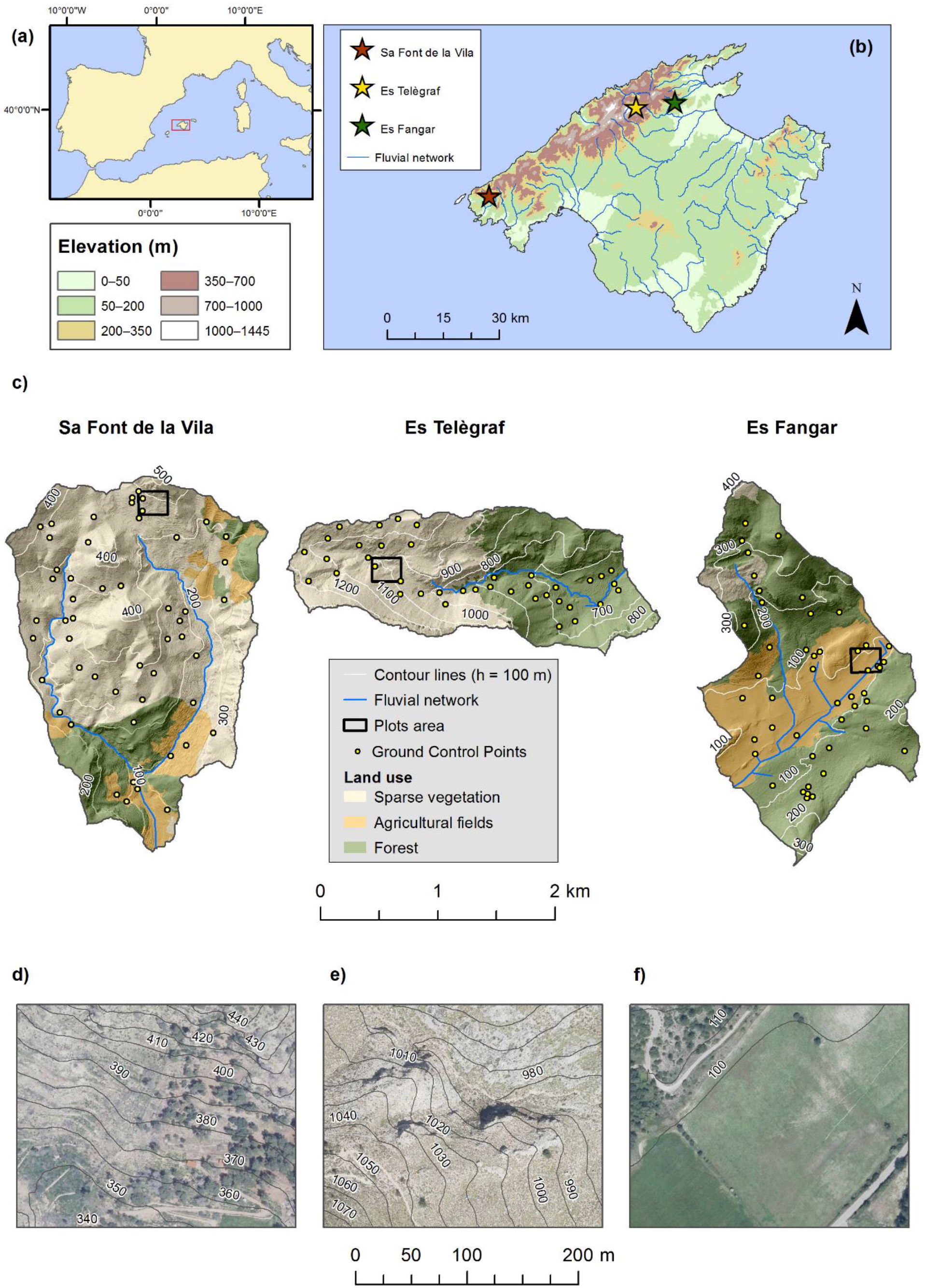
2. Study Area
3. Materials and Methods
3.1. DTM Datasets
3.2. Vertical Accuracy Assesment
3.3. Quality Assessment of DTMs for Hydrogeomorphological Modelling
4. Results
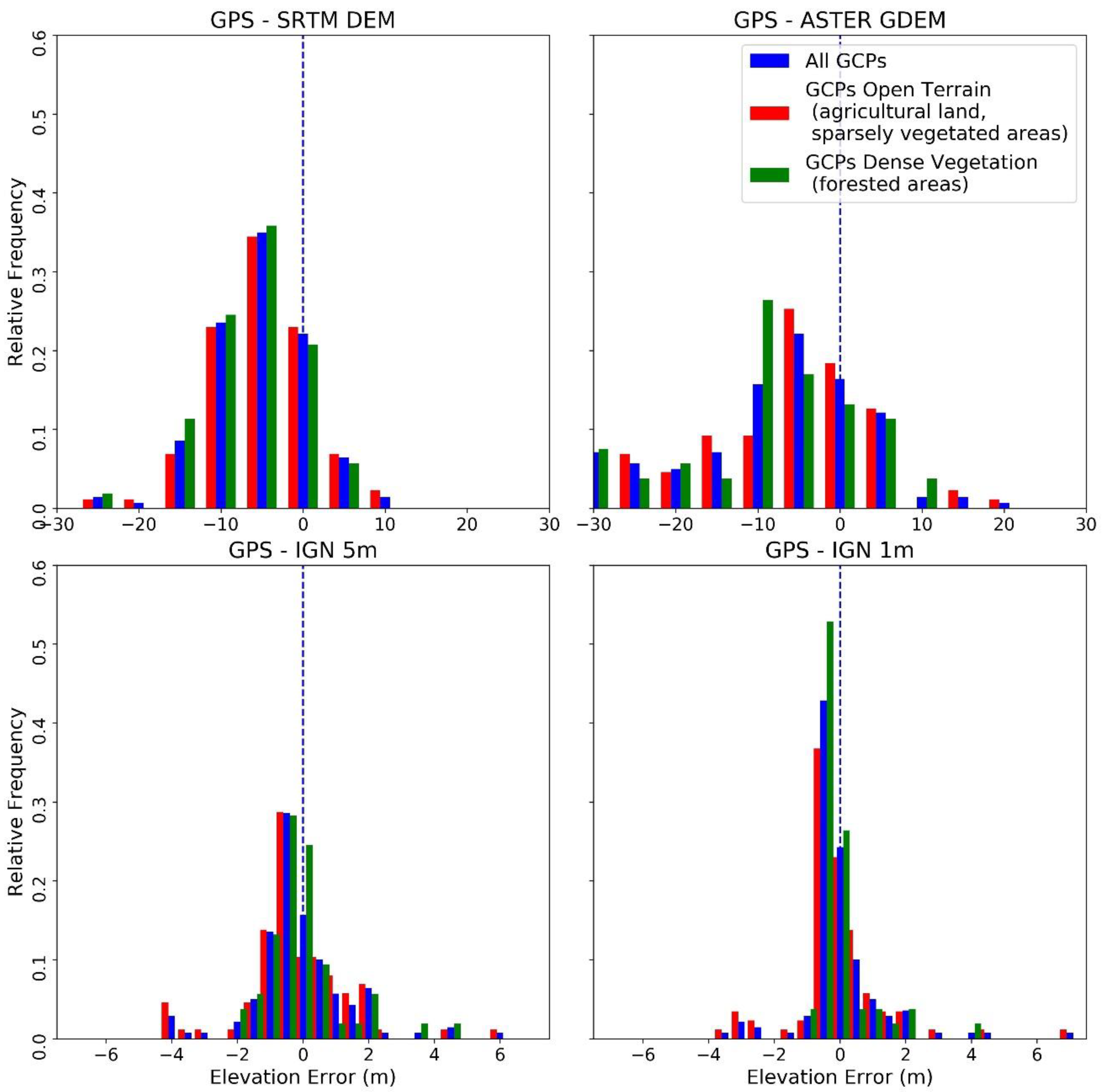
4.1. DTM Vertical Accuracy
4.2. DTM Hydrogeomorphic Modelling Performance
4.2.1. Basic Terrain Statistics
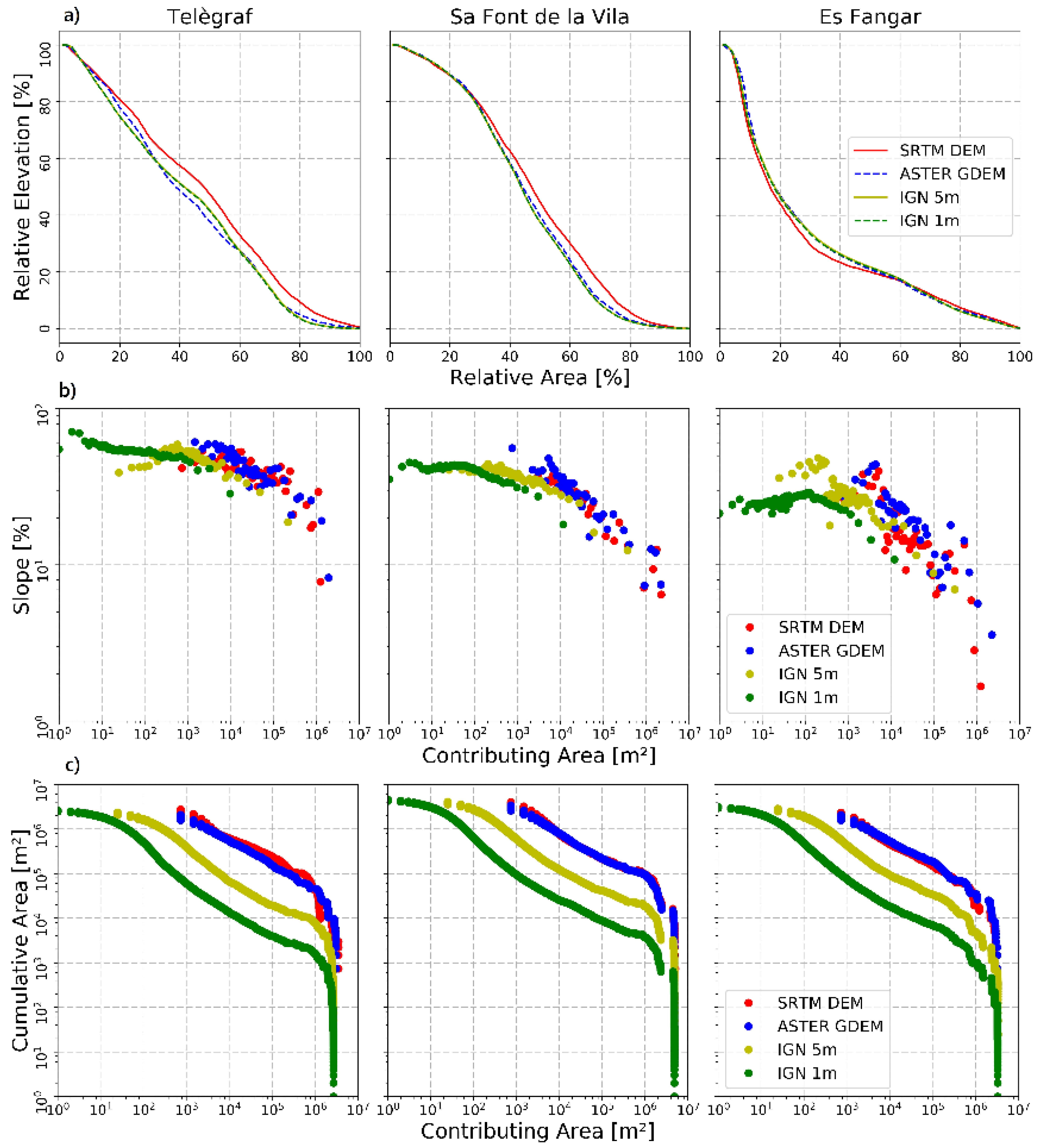
4.2.2. Geomorphometric Parameters and Relationships
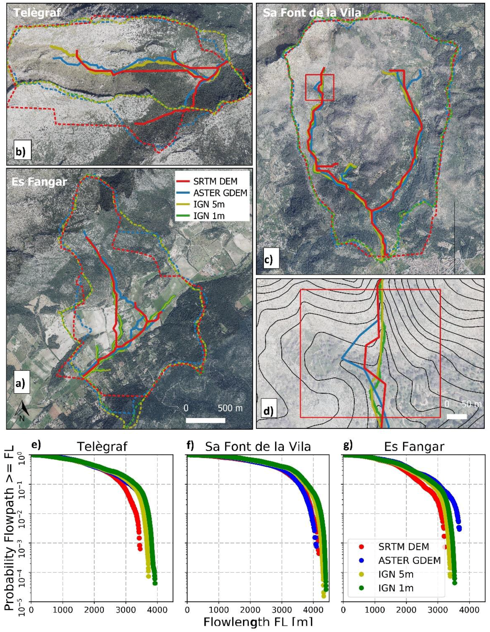
4.2.3. Stream Networks
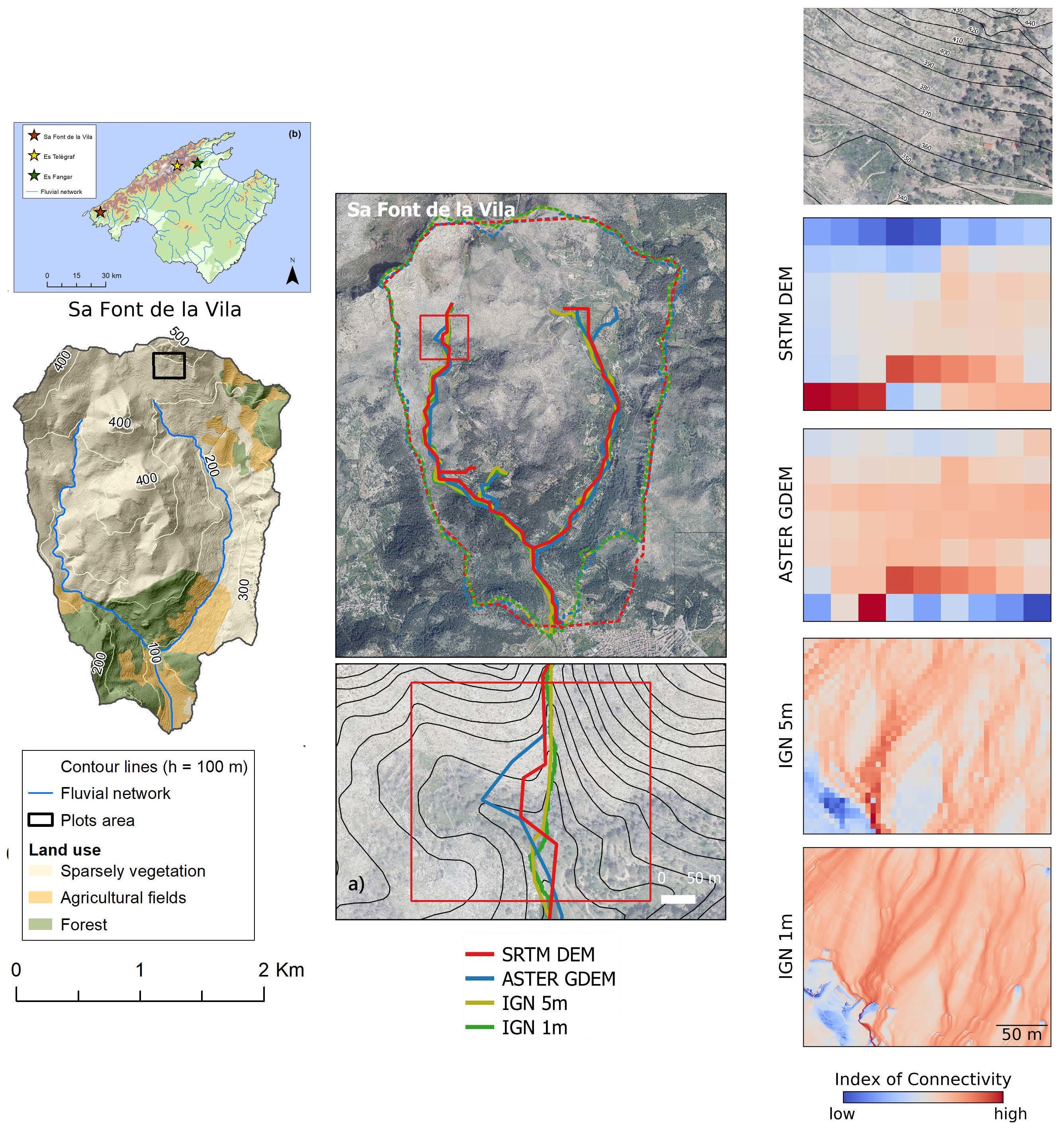
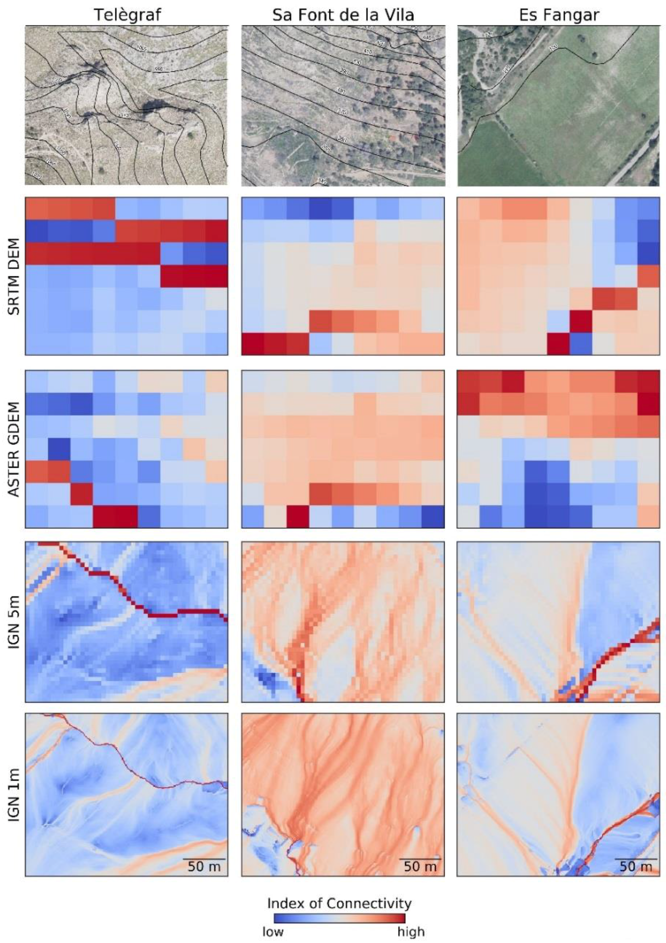
4.2.4. Small-Detail Water and Sediment Connectivity
5. Discussion
5.1. Vertical Accuracy
5.1.1. General Dataset Evaluation
5.1.2. Assessing the Effects of Vegetation on the Datasets
5.1.3. Evaluating Terrain Morphology on DTM Accuracy
5.2. Assessing Hydrogeomorphological Modelling Reliability
5.2.1. Basic Terrain Attributes
5.2.2. Geomorphic Parameters and Relationships
5.2.3. Stream Network Organisation
5.2.4. Small-Detail Arrangement Patterns of Water and Sediment Fluxes
6. Conclusions
- The analysed LiDAR-based models and—to a lower extent—SRTM provided reliable sources for most of the discussed hydrological and geomorphological modelling aspects. However, SRTM notably failed to produce reliable results for highly rugged, mountainous areas due to intrinsic errors associated with topographic RADAR shadowing effects. For the analysed LiDAR-based models, attention should be also paid to the influence of data processing steps such as grid interpolation and point-cloud classification.
- ASTER showed the lowest vertical accuracy and considerable residual artefacts producing strong, non-normally distributed elevation errors that largely constrained the reliability of the ASTER elevation data. The presence of forest vegetation exacerbated the tendency of the ASTER dataset to overestimate elevation values (accounting for up to 30-m deviations), although the inherent, large vertical errors that affected this dataset largely surpassed the influence of Mediterranean dry forest vegetation in measured absolute vertical accuracy.
- Intrinsic errors and scarcity of the underlying DTM production data, vegetation patterns, and complex terrain morphology as well as relief fragmentation (especially for Mediterranean landscapes with traditional terraced structures) influenced the analysed datasets to different extents, resulting in significant deviations of elevation values.
- Both the vertical accuracy and horizontal resolution of the datasets were found to influence catchment hydrogeomorphological modelling in the studied sites. Error propagation impacted flow routing, stream network, and catchment delineation, and to a lower extent, the distribution of slope gradient values. Coarse horizontal raster resolution was found to reduce the degree of hydrological and geomorphological detail available from the DTMs and their reliability in representing processes at different spatial scales within the catchment.
Author Contributions
Funding
Conflicts of Interest
References
- Florinsky, I.V. An illustrated introduction to general geomorphometry. Prog. Phys. Geogr. 2017, 41, 723–752. [Google Scholar] [CrossRef]
- Quinn, P.F.B.J.; Beven, K.; Chevallier, P.; Planchon, O. The Prediction of Hillslope Flow Paths for Distributed Hydrological Modelling Using Digital Terrain Models. Hydrol. Process. 1991, 5, 59–79. [Google Scholar] [CrossRef]
- Brasington, J.; Richards, K. Interactions between model predictions, parameters and DTM scales for TOPMODEL. Comput. Geosci. 1998, 24, 299–314. [Google Scholar] [CrossRef]
- Casas, A.; Benito, G.; Thorndycraft, V.R.; Rico, M. The topographic data source of digital terrain models as a key element in the accuracy of hydraulic flood modelling. Earth Surf. Process. Landf. 2006, 31, 444–456. [Google Scholar] [CrossRef]
- Sanders, F.B. Evaluation of on-line DEMs for flood inundation modeling. Adv. Water Resour. 2007, 30, 1831–1843. [Google Scholar] [CrossRef]
- Moore, I.D.; Grayson, R.B.; Ladson, A.R. Digital Terrain Modeling: A Review of Hydrological Geomorphological and Biological Applications. Hydrol. Process. 1991, 5, 3–30. [Google Scholar] [CrossRef]
- Florinsky, I. Errors of signal processing in digital terrain modelling. Int. J. Geogr. Inf. Sci. 2002, 16, 475–501. [Google Scholar] [CrossRef]
- Zhang, W.; Montgomery, D.R. Digital elevation model grid size, landscape representation, and hydrological simulations. Water Resour. Res. 1994, 30, 1019–1028. [Google Scholar] [CrossRef]
- Armstrong, R.N.; Martz, L.W. Topographic parameterization in continental hydrology: A study in scale. Hydrol. Process. 2003, 17, 3763–3781. [Google Scholar] [CrossRef]
- Hancock, G.R. The use of digital elevation models in the identification and characterization of catchments over different grid scales. Hydrol. Process. 2005, 19, 1727–1749. [Google Scholar] [CrossRef]
- Wu, S.; Li, J.; Huang, G.H. A study on DEM-derived primary topographic attributes for hydrologic applications: Sensitivity to elevation data resolution. Appl. Geogr. 2008, 28, 210–223. [Google Scholar] [CrossRef]
- Kenward, T.; Lettenmaier, D.P.; Wood, E.F.; Fielding, E. Effects of digital elevation model accuracy on hydrologic prediction. Remote Sens. Environ. 2000, 74, 432–444. [Google Scholar] [CrossRef]
- Merwade, V.; Olivera, F.; Arabi, M.; Edleman, S. Uncertainty in Flood Inundation Mapping: Current Issues and Future Directions. J. Hydrol. Eng. 2008, 13, 608–620. [Google Scholar] [CrossRef]
- Guth, P.L. Geomorphometric Comparison of ASTER GDEM and SRTM. In Proceedings of the A Special Joint Symposium of ISPRS Technical Commission IV & AutoCarto in Conjunction with ASPRS/CaGIS 2010 Fall Specialty Conference, Orlando, FL, USA, 15–19 November 2010. [Google Scholar]
- van Zyl, J.J. The Shuttle Radar Topography Mission (SRTM): A breakthrough in remote sensing of topography. Acta Astronaut. 2001, 48, 559–565. [Google Scholar] [CrossRef]
- Tachikawa, T.; Hat, M.; Kaku, M.; Iwasaki, A. Characteristics of ASTER GDEM version 2. In Proceedings of the 2011 IEEE International Geosciences Remote Sensing Symposium (IGARSS), Vancouver, BC, Canada, 24–29 July 2011; pp. 3657–3660. [Google Scholar] [CrossRef]
- Rabus, B.; Eineder, M.; Roth, A.; Bamler, R. The shuttle radar topography mission—A new class of digital elevation models acquired by spaceborne radar. ISPRS J. Photogramm. Remote Sens. 2003, 57, 241–262. [Google Scholar] [CrossRef]
- ASTER-GDEM-Validation-Team. ASTER Global Digital Elevation Model Version 2—Summary of Validation Results; NASA - Earth Resources Observation and Science (EROS) Center: Sioux Falls, SD, USA, 2011.
- Hodgson, M.E.; Bresnahan, P. Accuracy of airborne LiDAR derived elevation: Empirical assessment and error budget. Photogramm. Eng. Remote Sens. 2004, 70, 331–339. [Google Scholar] [CrossRef]
- Heritage, G.L.; Milan, D.J.; Large, A.R.G.; Fuller, I.C. Influence of survey strategy and interpolation model on DEM quality. Geomorphology 2009, 112, 334–344. [Google Scholar] [CrossRef]
- Chen, Z.; Gao, B.; Devereux, B. State-of-the-Art: DTM Generation Using Airborne LIDAR Data. Sensors 2017, 17, 150. [Google Scholar] [CrossRef]
- Simpson, J.E.; Smith, T.E.L.; Wooster, M.J. Assessment of errors caused by forest vegetation structure in airborne LiDAR-derived DTMs. Remote Sens. 2017, 9, 1101. [Google Scholar] [CrossRef]
- Bossi, G.; Cavalli, M.; Crema, S.; Frigerio, S.; Quan Luna, B.; Mantovani, M.; Marcato, G.; Schenato, L.; Pasuto, A. Multi-temporal LiDAR-DTMs as a tool for modelling a complex landslide: A case study in the Rotolon catchment (eastern Italian Alps). Nat. Hazards Earth Syst. Sci. 2015, 15, 715–722. [Google Scholar] [CrossRef]
- Fernández, T.; Pérez, J.; Colomo, C.; Cardenal, J.; Delgado, J.; Palenzuela, J.; Irigaray, C.; Chacón, J. Assessment of the Evolution of a Landslide Using Digital Photogrammetry and LiDAR Techniques in the Alpujarras Region (Granada, Southeastern Spain). Geosciences 2017, 7, 32. [Google Scholar] [CrossRef]
- Kamps, M.T.; Bouten, W.; Seijmonsbergen, A.C. LiDAR and orthophoto synergy to optimize object-based landscape change: Analysis of an active landslide. Remote Sens. 2017, 9, 805. [Google Scholar] [CrossRef]
- Höfle, B.; Rutzinger, M. Topographic airborne LiDAR in geomorphology: A technological perspective. Z. Geomorphol. 2011, 55, 1–29. [Google Scholar] [CrossRef]
- Tarolli, P. Geomorphology High-resolution topography for understanding Earth surface processes: Opportunities and challenges. Geomorphology 2014, 216, 295–312. [Google Scholar] [CrossRef]
- Moreno-de-las-Heras, M.; Saco, P.M.; Willgoose, G.R. A Comparison of SRTM V4 and ASTER GDEM for Hydrological Applications in Low Relief Terrain. Photogramm. Eng. Remote Sens. 2012, 78, 7807. [Google Scholar] [CrossRef]
- Athmania, D.; Achour, H. External validation of the ASTER GDEM2, GMTED2010 and CGIAR-CSI-SRTM v4.1 free access digital elevation models (DEMs) in Tunisia and Algeria. Remote Sens. 2014, 6, 4600–4620. [Google Scholar] [CrossRef]
- Jarihani, A.A.; Callow, J.N.; McVicar, T.R.; Van Niel, T.G.; Larsen, J.R. Satellite-derived Digital Elevation Model (DEM) selection, preparation and correction for hydrodynamic modelling in large, low-gradient and data-sparse catchments. J. Hydrol. 2015, 524, 489–506. [Google Scholar] [CrossRef]
- Czubski, K.; Kozak, J.; Kolecka, N. Accuracy of SRTM-X and ASTER Elevation Data and its Influence on Topographical and Hydrological Modeling: Case Study of the Pieniny Mts. in Poland. Int. J. Geoinform. 2013, 9, 7–14. [Google Scholar]
- Mukherjee, S.; Joshi, P.K.; Mukherjee, S.; Ghosh, A.; Garg, R.D.; Mukhopadhyay, A. Evaluation of vertical accuracy of open source Digital Elevation Model (DEM). Int. J. Appl. Earth Obs. Geoinform. 2013, 21, 205–217. [Google Scholar] [CrossRef]
- Nascetti, A.; Di Rita, M.; Ravanelli, R.; Amicuzi, M.; Esposito, S.; Crespi, M. Free global DSM assessment on large scale areas exploiting the potentialities of the innovative google earth engine platform. Int. Arch. Photogramm. Remote Sens. Spat. Inf. Sci. 2017, 42, 627–633. [Google Scholar] [CrossRef]
- Gorokhovich, Y.; Voustianiouk, A. Accuracy assessment of the processed SRTM-based elevation data by CGIAR using field data from USA and Thailand and its relation to the terrain characteristics. Remote Sens. Environ. 2006, 104, 409–415. [Google Scholar] [CrossRef]
- Ludwig, R.; Schneider, P. Validation of digital elevation models from SRTM X-SAR for applications in hydrologic modeling. ISPRS J. Photogramm. Remote Sens. 2006, 60, 339–358. [Google Scholar] [CrossRef]
- Notebaert, B.; Verstraeten, G.; Govers, G.; Poesen, J. Qualitative and quantitative applications of LiDAR imagery in fluvial geomorphology. Earth Surf. Process. Landf. 2009, 34, 217–231. [Google Scholar] [CrossRef]
- Sharma, A.; Tiwari, K.N. A comparative appraisal of hydrological behavior of SRTM DEM at catchment level. J. Hydrol. 2014, 519, 1394–1404. [Google Scholar] [CrossRef]
- Tan, M.L.; Ficklin, D.L.; Dixon, B.; Ibrahim, A.L.; Yusop, Z.; Chaplot, V. Impacts of DEM resolution, source, and resampling technique on SWAT-simulated streamflow. Appl. Geogr. 2015, 63, 357–368. [Google Scholar] [CrossRef] [Green Version]
- Santillan, J.R.; Makinano-Santillan, M. Vertical accuracy assessment of 30-M. resolution ALOS, ASTER, and SRTM global DEMS over Northeastern Mindanao, Philippines. Int. Arch. Photogramm. Remote Sens. Spat. Inf. Sci. 2016, 41, 149–156. [Google Scholar] [CrossRef]
- Nikolakopoulos, K.G.; Kamaratakis, E.K.; Chrysoulakis, N. SRTM vs ASTER elevation products. Comparison for two regions in Crete, Greece. Int. J. Remote Sens. 2006, 27, 4819–4838. [Google Scholar] [CrossRef]
- de Vente, J.; Poesen, J.; Govers, G.; Boix-Fayos, C. The implications of data selection for regional erosion and sediment yield modelling. Earth Surf. Process. Landf. 2009, 34, 1994–2007. [Google Scholar] [CrossRef]
- de Carvalho Júnior, O.A.; Guimarães, R.F.; Montgomery, D.R.; Gillespie, A.R.; Gomes, R.A.T.; de Souza Martins, É.; Silva, N.C. Karst depression detection using ASTER, ALOS/PRISM and SRTM-derived digital elevation models in the Bambuí group, Brazil. Remote Sens. 2013, 6, 330–351. [Google Scholar] [CrossRef]
- Hooke, J.M. Human impacts on fluvial systems in the Mediterranean region. Geomorphology 2006, 79, 311–335. [Google Scholar] [CrossRef]
- Iglesias, A.; Garrote, L.; Flores, F.; Moneo, M. Challenges to manage the risk of water scarcity and climate change in the Mediterranean. Water Resour. Manag. 2007, 21, 775–788. [Google Scholar] [CrossRef]
- Calsamiglia, A.; Lucas-Borja, M.E.; Fortesa, J.; García-Comendador, J.; Estrany, J. Changes in Soil Quality and Hydrological Connectivity Caused by the Abandonment of Terraces in a Mediterranean Burned Catchment. Forests 2017, 8, 333. [Google Scholar] [CrossRef]
- Serra, P.; Pons, X.; Saurı, D. Land-cover and land-use change in a Mediterranean landscape: A spatial analysis of driving forces integrating biophysical and human factors. Appl. Geogr. 2008, 28, 189–209. [Google Scholar] [CrossRef]
- Buendia, C.; Bussi, G.; Tuset, J.; Vericat, D.; Sabater, S.; Palau, A.; Batalla, R.J. Effects of afforestation on runoff and sediment load in an upland Mediterranean catchment. Sci. Total Environ. 2015, 540, 144–157. [Google Scholar] [CrossRef] [PubMed]
- Borselli, L.; Cassi, P.; Torri, D. Prolegomena to sediment and flow connectivity in the landscape: A GIS and field numerical assessment. Catena 2008, 75, 268–277. [Google Scholar] [CrossRef]
- Cavalli, M.; Trevisani, S.; Comiti, F.; Marchi, L. Geomorphometric assessment of spatial sediment connectivity in small Alpine catchments. Geomorphology 2013, 188, 31–41. [Google Scholar] [CrossRef]
- Gelabert, B.; Sabat, F.; Rodriguez-Perea, A. A structural outline of the Serra de Tramuntana of Mallorca (Balearic Islands). Tectonophysics 1992, 203, 167–183. [Google Scholar] [CrossRef]
- Calsamiglia, A.; Fortesa, J.; García-Comendador, J.; Lucas-Borja, M.; Calvo-Cases, A.; Estrany, J. Spatial patterns of sediment connectivity in terraced lands: Anthropogenic controls of catchment sensitivity. Land Degrad. Dev. 2018, 29, 1198–1210. [Google Scholar] [CrossRef]
- Koutsias, N.; Arianoutsou, M.; Kallimanis, A.S.; Mallinis, G.; Halley, J.M.; Dimopoulos, P. Where did the fires burn in Peloponnisos, Greece the summer of 2007? Evidence for a synergy of fuel and weather. Agric. For. Meteorol. 2012, 156, 41–53. [Google Scholar] [CrossRef]
- Rosselló-Verger, V.M. The Serra de Tramuntana of Mallorca. Phys. Hum. Orig. Source: Catalan Soc. Sci. Rev. 2014, 4, 15–30. [Google Scholar] [CrossRef]
- Estrany, J.; Garcia, C.; Martínez-Carreras, N.; Walling, D.E. A suspended sediment budget for the agricultural Can Revull catchment (Mallorca, Spain). Z. Geomorphol. Suppl. 2012, 56, 169–193. [Google Scholar] [CrossRef]
- Eineder, M.; Bamler, R.; Werner, M.; Rabus, B.; Breit, H.; Adam, N.; Suchandt, S.; Holzner, J. SRTM/X-SAR CALIBRATION STATUS. In Proceedings of the CEOS WGCV-SAR Workshop, Sydney, NSW, Australia, 9–13 July 2001. [Google Scholar]
- Rosen, P.A.; Hensley, S.; Gurrola, E.; Rogez, F.; Chan, S.; Martin, J.; Rodriguez, E. SRTM C-Band Topographic Data: Quality Assessments and Calibration Activities. In Proceedings of the IEEE 2001 International Geoscience and Remote Sensing Symposium, Sydney, Ausralia, 9–13 July 2001; Volume 2. [Google Scholar]
- Reuter, H.I.; Nelson, A.; Strobl, P.; Mehl, W.; Jarvis, A. A first assessment of ASTER GDEM tiles for absolute accuracy, relative accuracy and terrain parameters. In Proceedings of the IGARSS 2009 International Geosciences Remote Sensing Symposium, Capetown, South Africa, 13–17 July 2009; Volume 5, pp. 240–243. [Google Scholar]
- Szabó, G.; Singh, S.K.; Szabó, S. Slope angle and aspect as influencing factors on the accuracy of the SRTM and the ASTER GDEM databases. Phys. Chem. Earth Parts 2015, 83–84, 137–145. [Google Scholar] [CrossRef]
- IGN. Instituto Geográfico Nacional—Centro Nacional de Información Geográfica [WWW Document]. 2018. Available online: http://www.ign.es/web/ign/portal (accessed on 13 February 2018).
- Bashfield, A.; Keim, A. Continent-wide DEM Creation for the European Union. In Proceedings of the 34th International Symposium on Remote Sensing of Environment—The GEOSS Era: Towards Operational Environmental Monitoring, Sydney, Australia, 10–15 April 2011; pp. 10–15. [Google Scholar]
- Lee, S.; Wolberg, G.; Shin, S.Y. Scattered Data Interpolation with Multilevel, B-Splines. IEEE Trans. Vis. Comput. Gr. 1997, 3, 228–244. [Google Scholar] [CrossRef]
- Lee, J.S. Digital image enhancement and noise filtering by use of local statistics. IEEE Trans. Pattern Anal. Mach. Intell. 1980, 2, 165–168. [Google Scholar] [CrossRef] [PubMed]
- Höhle, J.; Höhle, M. Accuracy assessment of digital elevation models by means of robust statistical methods. ISPRS J. Photogramm. Remote Sens. 2009, 64, 398–406. [Google Scholar] [CrossRef] [Green Version]
- Höhle, J. The Assessment of the Absolute Planimetric Accuracy of Airborne Laserscanning. ISPRS—Int. Arch. Photogramm. Remote Sens. Spat. Inf. Sci. 2012, 145–150. [Google Scholar] [CrossRef]
- Planchon, O.; Darboux, F. A fast, simple and versatile algorithm to fill the depressions of digital elevation models. Catena 2001, 46, 159–176. [Google Scholar] [CrossRef]
- O’Callaghan, J.F.; Mark, D.M. The extraction of drainage networks from digital elevation data. Comput. Vis. Gr. Image Process. 1984, 27, 247. [Google Scholar] [CrossRef]
- Strahler, A.N. Hypsometric (Area-Altitude) Analysis of Erosional Topography. Geol. Soc. Am. Bull. 1952, 63, 1117–1142. [Google Scholar] [CrossRef]
- Hancock, G.R.; Martinez, C.; Evans, K.G.; Moliere, D.R. A comparison of SRTM and high-resolution digital elevation models and their use in catchment geomorphology and hydrology: Australian examples. Earth Surf. Process. Landf. 2006, 31, 1384–1412. [Google Scholar] [CrossRef]
- Willgoose, G.R. A physical explanation for an observed area-slope-elevation relationship for declining catchments. Water Resour. Res. 1994, 30, 151–159. [Google Scholar] [CrossRef]
- Rodríguez-Iturbe, I.; Ijjász-Vásquez, E.; Bras, R.; Tarboton, D. Power law distributions of discharge mass and energy in River Basins. Water Resour. Res. 1992, 28, 1089–1093. [Google Scholar] [CrossRef]
- Vivoni, E.R.; Di Benedetto, F.; Grimaldi, S.; Eltahir, E.A. Hypsometric Control on Surface and Subsurface Runoff. Water Resour. Res. 2008, 44, 12502–12511. [Google Scholar] [CrossRef]
- Strahler, A.N. Quantitative analysis of watershed geomorphology. Trans. Am. Geophys. Union 1957, 38, 913–920. [Google Scholar] [CrossRef]
- Roering, J.J.; Perron, J.T.; Kirchner, J.W. Functional relationships between denudation andhillslope form and relief. Earth Planet. Sci. Lett. 2007, 264, 245–258. [Google Scholar] [CrossRef]
- Perera, H.; Willgoose, G.R. A physical explanation of the cumulative area distribution curve. Water Resour. Res. 1998, 34, 1335–1343. [Google Scholar] [CrossRef] [Green Version]
- Moglen, G.E.; Bras, R.L. The importance of spatially heterogeneous erosivity and the cumulative area distribution within a basin evolution model. Geomorphology 1995, 12, 173–185. [Google Scholar] [CrossRef]
- Wischmeier, W.H.; Smith, D.D. Predicting rainfall erosion losses A guide to conservation planning. Agric. Handb. 1978, 537. [Google Scholar]
- Desmet, P.J.; Govers, G. A GIS procedure for automatically calculating the USLE LS factor on topographically complex landscape units. J. Soil Water Conserv. 1996, 51, 427–433. [Google Scholar]
- Conrad, O.; Bechtel, B.; Dietrich, H.; Fischer, E.; Gerlitz, L.; Wehberg, J.; Wichmann, V.; Boehner, J. System for Automated Geoscientific Analyses (SAGA) v. 2.1.4. Geosci. Model Dev. 2015, 8, 1991–2007. [Google Scholar] [CrossRef]
- Wainwright, J.; Turnbull, L.; Ibrahim, T.G.; Lexartza-Artza, I.; Thornton, S.F.; Brazier, R.E. Linking environmental regimes, space and time: Interpretations of structural and functional connectivity. Geomorphology 2011, 126, 387–404. [Google Scholar] [CrossRef]
- Crema, S.; Cavalli, M. SedInConnect: A stand-alone, free and open source tool for the assessment of sediment connectivity. Comput. Geosci. 2018, 111, 39–45. [Google Scholar] [CrossRef]
- Li, P.; Shi, C.; Li, Z.; Muller, J.P.; Drummond, J.; Li, X.; Li, T.; Li, Y.; Liu, J. Evaluation of ASTER GDEM VER2 using GPS measurements and SRTM VER4.1 in China. ISPRS Ann. Photogramm. Remote Sens. Spat. Inf. Sci. 2012, 1–4, 181–186. [Google Scholar] [CrossRef]
- Estornell, J.; Ruiz, L.A.; Velázquez-Martí, B.; Hermosilla, T. Analysis of the factors affecting lidar dtm accuracy in a steep shrub area. Int. J. Dig. Earth 2011, 4, 521–538. [Google Scholar] [CrossRef]
- Clark, M.L.; Clark, D.B.; Roberts, D.A. Small-footprint lidar estimation of sub-canopy elevation and tree height in a tropical rain forest landscape. Remote Sens. Environ. 2004, 91, 68–89. [Google Scholar] [CrossRef]
- Meng, X.; Currit, N.; Zhao, K. Ground filtering algorithms for airborne LiDAR data: A review of critical issues. Remote Sens. 2010, 2, 833–860. [Google Scholar] [CrossRef]
- Bater, C.W.; Coops, N.C. Evaluating error associated with lidar-derived DEM interpolation. Comput. Geosci. 2009, 35, 289–300. [Google Scholar] [CrossRef]
- Aguilar, F.J.; Mills, J.P.; Delgado, J.; Aguilar, M.A.; Negreiros, J.G.; Pérez, J.L. Modelling vertical error in LiDAR-derived digital elevation models. ISPRS J. Photogramm. Remote Sens. 2010, 65, 103–110. [Google Scholar] [CrossRef]
- Kellndorfer, J.; Walker, W.; Pierce, L.; Dobson, C.; Fites, J.A.; Hunsaker, C.; Vona, J.; Clutter, M. Vegetation height estimation from Shuttle Radar Topography Mission and National Elevation Datasets. Remote Sens. Environ. 2004, 93, 339–358. [Google Scholar] [CrossRef]
- Carabajal, C.C.; Harding, D.J. SRTM C-Band and ICEsat Laser Altimetry Elevation Comparisons as a Function of Tree Cover and Relief. Photogramm. Eng. Remote Sens. 2006, 72, 287–298. [Google Scholar] [CrossRef]
- Walker, W.S.; Kellndorfer, J.M.; Pierce, L.E. Quality assessment of SRTM C- and X-band interferometric data: Implications for the retrieval of vegetation canopy height. Remote Sens. Environ. 2007, 106, 428–448. [Google Scholar] [CrossRef]
- Harding, D.J.; Lefsky, M.A.; Parker, G.G.; Blair, J.B. Laser altimeter canopy height profiles methods and validation for closed-canopy, broadleaf forests. Remote Sens. Environ. 2001, 76, 283–297. [Google Scholar] [CrossRef]
- Eineder, M. Problems and Solutions for INSAR Digital Elevation Model Generation of Mountainous Terrain. In Proceedings of the FRINGE 2003 Workshop, Frascatti, Italy, 1–5 December 2003. [Google Scholar]
- Nascetti, A.; Capaldo, P.; Porfiri, M.; Pieralice, F.; Fratarcangeli, F.; Benenati, L.; Crespi, M. Fast terrain modelling for hydrogeological risk mapping and emergency management: The contribution of high-resolution satellite SAR imagery. Geomat. Nat. Hazards Risk 2015, 6, 554–582. [Google Scholar] [CrossRef]
- Arefi, H.; Reinartz, P. Accuracy enhancement of ASTER global digital elevation models using ICESat data. Remote Sens. 2011, 3, 1323–1343. [Google Scholar] [CrossRef]
- Liu, X. Airborne LiDAR for DEM generation: Some critical issues. Prog. Phys. Geogr. 2008, 32, 31–49. [Google Scholar] [CrossRef]
- Pérez-Peña, J.V.; Azañón, J.M.; Booth-Rea, G.; Azor, A.; Delgado, J. Differentiating geology and tectonics using a spatial autocorrelation technique for the hypsometric integral. J. Geophys. Res. Earth Surf. 2009, 114. [Google Scholar] [CrossRef] [Green Version]
- Kienzle, S. The Effect of DEM Raster Resolution on First Order, Second Order and Compound Terrain Derivatives. Trans. GIS 2004, 8, 83–111. [Google Scholar] [CrossRef]
- Fryirs, K.A. River sensitivity: A lost foundation concept in fluvial geomorphology. Earth Surf. Process. Landf. 2017, 42, 55–70. [Google Scholar] [CrossRef]
- Wu, S.; Li, J.; Huang, G. An evaluation of grid size uncertainty in empirical soil loss modeling with digital elevation models. Environ. Model. Assess. 2005, 10, 33–42. [Google Scholar] [CrossRef]
- McMaster, K.J. Effects of digital elevation model resolution on derived stream network positions. Water Resour. Res. 2002, 38. [Google Scholar] [CrossRef]
- Oksanen, J.; Sarjakoski, T. Error propagation analysis of DEM-based drainage basin delineation. Int. J. Remote Sens. 2005, 26, 3085–3102. [Google Scholar] [CrossRef]
- Chaubey, I.; Cotter, A.S.; Costello, T.A.; Soerens, T.S. Effect of DEM data resolution on SWAT output uncertainty. Hydrol. Process. 2005, 19, 621–628. [Google Scholar] [CrossRef] [Green Version]
- Calsamiglia, A.; Garcia-Comendador, J.; Fortesa, J.; López-Tarazón, J.A.; Crema, S.; Cavalli, M.; Calvo-Cases, A.; Estrany, J. Effects of agricultural drainage systems on sediment connectivity in a small Mediterranean lowland catchment. Geomorphology 2018, 318, 162–171. [Google Scholar] [CrossRef]


| Hydrogeomorphological Statistics and Descriptors | References |
|---|---|
| Basic terrain characteristics | |
| Minimum, maximum, mean elevation, and total relief | |
| Mean and SD of slope gradient | |
| Mean and SD (D8*) of flowlength | O’Callaghan and Marks [66] |
| Total catchment area | O’Callaghan and Marks [66] |
| Catchment geomorphometric parameters and relationships | |
| Terrain hypsometry | Strahler [67] |
| Slope–area relationship | Hancock et al. [68], Willgoose [69] |
| Cumulative area distribution | Rodríguez-Iturbe et al. [70] |
| Mean and SD of LS** factor | Wischmeier and Smith [76], Desmet and Govers [77] |
| Stream network and flowpath properties | |
| Stream network patterns | O’Callaghan and Marks [66] |
| Cumulative distribution function of flowpath lengths | Moreno-de-las-Heras et al. [28] |
| Small-detail water/sediment flow arrangement patterns | |
| Surface connectivity index (IC) | Borselli et al. [48], Cavalli et al. [49] |
| SRTM DEM | ASTER GDEM | IGN 5 m | IGN 1 m | |
|---|---|---|---|---|
| All sites (n = 140) | ||||
| RMSE | 6.98 | 16.10 | 1.73 | 1.55 |
| NMAD | 5.27 | 11.23 | 0.84 | 0.44 |
| All open terrain sites (agricultural + sparse vegetation cover, n = 87) | ||||
| RMSE | 7.38 | 16.26 | 1.59 | 1.41 |
| NMAD | 5.22 | 10.82 | 0.93 | 0.61 |
| All densely vegetated sites (forest cover, n = 53) | ||||
| RMSE | 6.28 | 15.84 | 1.94 | 1.76 |
| NMAD | 5.31 | 11.46 | 0.73 | 0.33 |
| Sa Font de la Vila catchment (n = 53) | ||||
| RMSE | 8.28 | 9.62 | 2.09 | 2.03 |
| NMAD | 5.59 | 7.63 | 0.98 | 0.62 |
| Es Telègraf catchment (n = 40) | ||||
| RMSE | 7.76 | 26.77 | 1.59 | 1.25 |
| NMAD | 5.76 | 12.17 | 0.89 | 0.49 |
| Es Fangar catchment (n = 47) | ||||
| RMSE | 4.06 | 7.62 | 1.35 | 1.10 |
| NMAD | 2.98 | 7.72 | 0.71 | 0.26 |
| SRTM DEM | ASTER GDEM | IGN 5 m | IGN 1 m | ||||||
|---|---|---|---|---|---|---|---|---|---|
| Uncorr | Corr | Uncorr | Corr | Uncorr | Corr | Uncorr | Corr | ||
| Sa Font de la Vila | Minimum Elevation (m) | 71.5 | 71.5 | 71.0 | 71.0 | 66.6 | 66.6 | 66.0 | 66.3 |
| Maximum Elevation (m) | 470.0 | 470.0 | 505.0 | 505.0 | 516.1 | 516.1 | 516.4 | 516.4 | |
| Mean Elevation (m) | 252.7 | 252.7 | 257.8 | 257.8 | 256.7 | 256.7 | 256.4 | 256.7 | |
| Mean Slope (%) | 30.9 | 30.8 | 33.4 | 33.1 | 39.7 | 39.7 | 40.5 | 40.5 | |
| Relief (m) | 398.5 | 398.5 | 434.0 | 434.0 | 449.5 | 449.5 | 449.8 | 450.1 | |
| Catchment Area (km2) | - | 5.06 | - | 4.83 | - | 4.82 | - | 4.83 | |
| Filtered Area (%) | - | 0.2 | - | 0.6 | - | <0.1 | - | <0.1 | |
| Es Telègraf | Minimum Elevation (m) | 638.5 | 638.5 | 632.0 | 639.0 | 625.0 | 625.0 | 624.6 | 624.6 |
| Maximum Elevation (m) | 1337.5 | 1337.5 | 1350.0 | 1350.0 | 1349.5 | 1349.5 | 1351.0 | 1351.0 | |
| Mean Elevation (m) | 947.4 | 947.4 | 921.4 | 921.4 | 912.7 | 912.7 | 911.6 | 911.6 | |
| Mean Slope (%) | 44.7 | 44.7 | 45.4 | 45.2 | 54.2 | 54.2 | 55.6 | 55.6 | |
| Relief (m) | 699.0 | 699.0 | 718.0 | 711.0 | 724.5 | 724.5 | 726.4 | 726.4 | |
| Catchment Area (km2) | - | 3.55 | - | 3.17 | - | 2.73 | - | 2.72 | |
| Filtered Area (%) | - | 0.1 | - | 0.7 | - | <0.1 | - | <0.1 | |
| Es Fangar | Minimum Elevation (m) | 74.3 | 74.9 | 70.0 | 74.0 | 73.0 | 73.4 | 73.2 | 73.9 |
| Maximum Elevation (m) | 369.9 | 369.9 | 405.0 | 405.0 | 403.8 | 403.8 | 403.9 | 403.9 | |
| Mean Elevation (m) | 157.8 | 157.8 | 163.6 | 163.7 | 163.0 | 163.0 | 162.7 | 162.7 | |
| Mean Slope (%) | 18.8 | 18.8 | 22.3 | 21.9 | 23.8 | 23.8 | 24.3 | 24.3 | |
| Relief (m) | 295.6 | 295.0 | 335.0 | 331.0 | 330.8 | 330.4 | 330.7 | 330.0 | |
| Catchment Area (km2) | - | 3.04 | - | 3.26 | - | 3.42 | - | 3.39 | |
| Filtered Area (%) | - | 0.3 | - | 1.7 | - | <0.1 | - | <0.1 | |
| SRTM DEM | ASTER GDEM | IGN 5 m | IGN 1 m | ||
|---|---|---|---|---|---|
| Sa Font de la Vila | Hypsometric Integral (-) | 0.46 | 0.44 | 0.43 | 0.43 |
| Mean Flowlength (m) | 2304.3 | 2344.4 | 2520.2 | 2566.9 | |
| SD Flowlength (m) | 1020.1 | 969.3 | 1011.5 | 1031.0 | |
| Mean LS factor (-) | 5.4 | 4.8 | 6.7 | 12.1 | |
| SD LS factor (-) | 2.8 | 3.2 | 11.1 | 24.0 | |
| Es Telègraf | Hypsometric Integral (-) | 0.45 | 0.41 | 0.41 | 0.41 |
| Mean Flowlength (m) | 1760.3 | 1820.6 | 1821.3 | 1877 | |
| SD Flowlength (m) | 814.4 | 902.7 | 950.2 | 991.8 | |
| Mean LS factor (-) | 7.4 | 5.3 | 9.7 | 18.1 | |
| SD LS factor (-) | 9.5 | 4.5 | 33.1 | 37.3 | |
| Es Fangar | Hypsometric Integral (-) | 0.27 | 0.28 | 0.28 | 0.28 |
| Mean Flowlength (m) | 1554.3 | 1789.3 | 1668.3 | 1731.0 | |
| SD Flowlength (m) | 711.0 | 867.3 | 791.8 | 826.1 | |
| Mean LS factor (-) | 3.3 | 3.6 | 4.5 | 9.1 | |
| SD LS factor (-) | 2.7 | 2.8 | 7.9 | 20.6 |
© 2018 by the authors. Licensee MDPI, Basel, Switzerland. This article is an open access article distributed under the terms and conditions of the Creative Commons Attribution (CC BY) license (http://creativecommons.org/licenses/by/4.0/).
Share and Cite
Graf, L.; Moreno-de-las-Heras, M.; Ruiz, M.; Calsamiglia, A.; García-Comendador, J.; Fortesa, J.; López-Tarazón, J.A.; Estrany, J. Accuracy Assessment of Digital Terrain Model Dataset Sources for Hydrogeomorphological Modelling in Small Mediterranean Catchments. Remote Sens. 2018, 10, 2014. https://0-doi-org.brum.beds.ac.uk/10.3390/rs10122014
Graf L, Moreno-de-las-Heras M, Ruiz M, Calsamiglia A, García-Comendador J, Fortesa J, López-Tarazón JA, Estrany J. Accuracy Assessment of Digital Terrain Model Dataset Sources for Hydrogeomorphological Modelling in Small Mediterranean Catchments. Remote Sensing. 2018; 10(12):2014. https://0-doi-org.brum.beds.ac.uk/10.3390/rs10122014
Chicago/Turabian StyleGraf, Lukas, Mariano Moreno-de-las-Heras, Maurici Ruiz, Aleix Calsamiglia, Julián García-Comendador, Josep Fortesa, José A. López-Tarazón, and Joan Estrany. 2018. "Accuracy Assessment of Digital Terrain Model Dataset Sources for Hydrogeomorphological Modelling in Small Mediterranean Catchments" Remote Sensing 10, no. 12: 2014. https://0-doi-org.brum.beds.ac.uk/10.3390/rs10122014