Geometric, Environmental and Hardware Error Sources of a Ground-Based Interferometric Real-Aperture FMCW Radar System

Abstract

Ground-based interferometric radar systems have numerous environmental monitoring applications in geoscience. Development of a relatively simple ground-based interferometric real-aperture FMCW radar (GB-InRAR) system that can be readily deployed in field without an established set of corner reflectors will meet the present and future need for real-time monitoring of the expected increased number of geohazard events due to climate changes. Several effects affect electromagnetic waves and limit the measurement accuracy, and a careful analysis of the setup of the deployed radar system in field is essential to achieve adequate results. In this paper, we present radar measurement of a moving square trihedral corner reflector from experiments conducted in both the field and laboratory, and assess the error sources with focus on the geometry, hardware and environmental effects on interferometric and differential interferometric measurements. A theoretical model is implemented to assess deviations between theory and measurements. The main observed effects are variations in radio refractivity, multipath interference and inter-reflector interference. Measurement error due to radar hardware and the environment are analyzed, as well as how the geometry of the measurement setup affects the nominal range-cell extent. It is found that for this experiment the deviation between interferometry and differential interferometry is mainly due to variations in the radio refractivity, and temperature-induced changes in the electrical length of the microwave cables. The results show that with careful design and analysis of radar parameters and radar system geometry the measurement accuracy of a GB-InRAR system without the use of deployed corner reflectors is comparable to the accuracy of differential interferometric measurements. A GB-InRAR system can therefore be used during sudden geo-hazard events without established corner reflector infrastructure, and the results are also valid for other high-precision interferometric radar systems.

1. Introduction

The all-weather capability of radar makes it the natural instrument for real-time monitoring in geosciences for potential life-threatening natural events like rock and mountain slides; clay and snow avalanches; volcanoes; open pit mines [1]; and structural monitoring of dam fronts [2], buildings and bridges [3,4,5]. The use of ground-based interferometric real aperture radar to measure unstable mountains [6,7,8,9], landslides [10], glacier movements, and calving events [11,12,13] gives good results. Experience from radar measurements shows that environmental and geometrical effects limit or have a great influence on the accuracy of the measurements. In a recent 8-year study of monitoring an unstable mountainside [6], it was found that atmospheric decorrelation was the major factor limiting the measurement accuracy when monitoring submillimeter motion at distances of 3 to 4 km. In this study and in Reference [8], it was shown that by introducing a reference reflector and by performing differential interferometry, most of the variations caused by atmospheric decorrelation were removed. However, it is not always possible to introduce radar reflectors due to the nature of the monitored area or from a safety point of view, typically for an unstable mountain with a lot of motion and occasional rock falls. In cases with unexpected geological hazards, it may not be possible to establish a set of corner reflectors. There is, therefore, a need for a thorough assessment of GB-InRAR systems, including radar hardware, measurement geometry and environmental effects, to find ways to compensate for the interferometric measurements for the environmental and geometrical effects in order to achieve accuracies comparable to differential interferometry.

Published literature on environmental variations on longtime geological monitoring with real-aperture radar are scarce as the main focus is on space-borne and ground-based Synthetic Aperture Radar (SAR); however, the environmental effects discussed in the literature are also for the use of Frequency Modulated Continuous Wave (FMCW) GB-InRAR systems. Atmospheric decorrelation was first observed in space-born SAR data when assessing slow subsidence rates [14]. To overcome the problem of atmospheric decorrelation, the Permanent Scatter (PS) Technique was developed [15], and a thorough analysis of the technique is given in Reference [16]. The technique utilizes time-coherent pixels to help bypass the geometrical and temporal decorrelation. Efficient techniques for compensation of GB-SAR based on statistical analysis of local meteorological data in combination with PS is reported in References [17,18,19,20]. In Reference [20] it was noted that compensating for atmospheric decorrelation due to temperature-induced turbulence and long distances is still a challenge. A recent study of Alpine glaciers in Italy and Spain reports an accuracy of a few millimeters/day when applying atmospheric phase screening (APS) corrections under challenging atmospheric conditions [13]. Accuracy improvements for real-aperture differential interferometric radar based on local meteorological data are reported in Reference [8].

One of the main differences between GB-SAR and real-aperture radar is the two-dimensional mapping capability of the GB-SAR system. The cost of 2D mapping is longer data acquisition time due to the mechanical motion of the antenna, which makes the GB-SAR system more sensitive to atmospheric and geometric decorrelation both during and between data acquisition. As stated in Reference [19], the time between data acquisition should be reduced as much as possible to avoid significant variation in the atmospheric conditions between measurements. Typical acquisition times of a GB-SAR-system are in the order of minutes while a typical real-aperture radar has a pulse repetition frequency (PRF) of a few thousand measurements per second. The high PRF of the real-aperture radar makes it easier to track and correct for atmospheric decorrelation due to the temporal variation in temperature, humidity and the pressure between measurements.

The geometry of the system must be considered carefully when deploying a GB-InRAR. When deploying an on-demand remote sensing system it is often time-critical to get the system operational and on-line. The choices of where to locate the radar are often restricted and the measurement geometry may deviate from an optimum radar measurement setup. If the radar is not radially directed against the anticipated motional direction of the monitored objects, the motion will be underestimated and must be corrected for. Another geometrical effect that may affect the measurement accuracy is multipath interference [21]. Multipath interference can occur when the energy radiated from the radar antenna hits a reflective surface, usually the ground, and is reflected towards the target. This additional signal adds coherently to the direct path signal and deteriorates the phase and magnitude of the data. It is stated in Reference ([22]; p. 2.31) that multipath interference is the most important non-free-space effect. A ripple in the amplitude of the backscatter from both stationary and moving objects is another geometric effect observed in high-resolution radar measurements of moving objects, where the data acquisition time is substantially faster than the velocity of the tracked object. This effect is probably coupled to the relative radar cross-section (RCS) value of the objects in the measurement area.

Environmental effects affect all radar system hardware, however, unlike a permanently installed remote sensing system an on-demand deployed system is more likely to be exposed to environmental variations as no infrastructure or environmental shielding can be expected to be present. The frequency and phase stability of microwave hardware is sensitive to variation in temperature, and this applies especially to oscillators and microwave cables. Uncorrected, this may lead to variations in the measured interferometric distance and a decrease in measurement accuracy. In Reference [23] it is stated that the temperature-induced phase shift in microwave cables is critical in high performance measurements. The magnitude of the phase-shift depends on the length of the cable and the operational temperature range of the radar system. The temperature-induced variation in the radar hardware should be separated from the temperature-induced environmental effects to avoid overcompensation of either effect.

A concern when measuring displacements without the use of reflectors is strong scatterers on the surface illuminated by the radar. Strong scatterers may be natural, e.g., stone blocks, or artificial, e.g., rockfall catch fences. Their presence may negatively affect the accuracy of the measurements as the strong back scatterers may interfere or shadow the backscatter from the other objects in the monitoring area. In Reference [24] it is stated that when monitoring in the presence of rockfall catch fences the interferometric phase information is not reliable. This is likely due to multiple effects like strong backscatter, shadowing and interference. In Reference [25] it is stated that GB-SAR is less suited for single-point monitoring than GB-InRAR in the presence of spatially-concentrated backscatter. This may be due to the azimuth width of the antennas, which for GB-SAR usually is much wider than for GB-InRAR, resulting in a larger illuminated area, hence, making the GB-SAR more vulnerable to cross-range interference. It is therefore of interest to assess the effect experimentally by tracking objects in the presence of stationary strong scatterers.

In this paper, we have investigated the effects influencing interferometric measurements of moving targets using a GB-InRAR, with a focus on applications in geosciences. Both controlled field and laboratory measurement experiments were set up to assess the effects influencing the measurement accuracy. In addition, a software model was developed to verify these effects. A series of experimental interferometric radar measurements were conducted on both stationary and moving targets. The purpose of the measurements was to gather information on how various environmental and geometric effects influenced the accuracy of the measurements, and to find a way to predict and correct for the effects, so that a relatively simple GB-InRAR system can be readily and optimally employed on site for field measurements.

This paper deals with five major effects influencing the accuracy of interferometric and differential interferometric radar measurements:

• The geometry of the measurement setup
• Atmospheric effects i.e., radio refractivity
• Effect of ground reflections i.e., multipath interference
• Radar target interference
• The radar hardware

The presented field results are utilizing the measured phase information registered by the GB-InRAR from the company ISPAS AS, and movements are calculated from phase differences based on the principle of interferometry. To exclude any systematic artifacts of the GB-InRAR, the laboratory measurements were all made using a Rhode & Schwarz Vector Network Analyzer (VNA).

In this paper, we start by outlining the radar theory necessary to analyze the measured data and to develop the numerical simulation model. We then describe the measurement setup and compare the field measurements with the results from the numeric model. Finally, we discuss the error sources and the factors limiting the accuracy of interferometric measurements and give some advice regarding setup and operational measurements.

2. Radar Theory and Implementation of Numerical Model

In this section, the theory for the implemented numerical simulation model and some of the radar theory that is used in the analysis of the measurements are presented.

2.1. Modeling of FMCW Radar Signals

A numerical simulation model was implemented, based on analytic expressions, to analyze and find deviations between theoretic and measured results. The transmitted radar signal is [26]

$$\mathrm{u}(\mathrm{t})={\mathrm{A}}_{\mathrm{u}}\cos {\mathsf{\phi }}_{\mathrm{u}}={\mathrm{A}}_{\mathrm{u}}\cos \left(2\mathsf{\pi }\left({\mathrm{f}}_0+\frac{\mathsf{\alpha }}{2}\mathrm{t}\right)\mathrm{t}+{\mathsf{\phi }}_0\right),$$

(1)

where A_u is the amplitude of the transmitted signal; f₀ is the frequency of the carrier; α is the ramp rate of the modulating signal; $\mathsf{\alpha }=\frac{\mathrm{BW}}{{\mathrm{T}}_{\mathrm{sweep}}}$ where BW is the bandwidth of the modulated signal, T_sweep is the modulation time and $\mathsf{\phi }$₀ is the initial phase of the transmitted signal. The received radar signal is [26]

$$\mathrm{z}(\mathrm{t})={\mathrm{A}}_{\mathrm{z}}\cos {\mathsf{\phi }}_{\mathrm{z}}={\mathrm{A}}_{\mathrm{z}}\cos \left(2\mathsf{\pi }\left({\mathrm{f}}_0+\frac{\mathsf{\alpha }}{2}(\mathrm{t}-\mathsf{\tau })\right)(\mathrm{t}-\mathsf{\tau })+{\mathsf{\phi }}_0\right),$$

(2)

where τ is the travel time of the electromagnetic wave. The received signal is split in two parts; one part is down-converted by in-phase and the second part by a 90°-shifted time delayed copy of the transmitted signal. The decomposition of the received signal in quadrature channels is [26]

$$\mathrm{I}(\mathrm{t})={\mathrm{A}}_{\mathrm{z}}^{\prime }\cos \left(2\mathsf{\pi }\left(\frac{\mathsf{\alpha }}{2}\mathsf{\tau }-\mathsf{\alpha }\mathrm{t}\right)\mathsf{\tau }\right),$$

(3)

$$\mathrm{Q}(\mathrm{t})={\mathrm{A}}_{\mathrm{z}}^{\prime }\sin \left(2\mathsf{\pi }\left(\frac{\mathsf{\alpha }}{2}\mathsf{\tau }-\mathsf{\alpha }\mathrm{t}\right)\mathsf{\tau }\right)$$

(4)

where I(t) is the in-phase part and Q(t) is the quadrature part of the signal. The amplitude and phase of the complex down-converted signal are

$$\mathrm{A}(\mathrm{t})=\sqrt{\mathrm{I}{\left(\mathrm{t}\right)}^2+\mathrm{Q}{\left(\mathrm{t}\right)}^2},$$

(5)

$$\mathsf{\phi }(\mathrm{t})={\tan }^{-1}\left(\frac{\mathrm{Q}\left(\mathrm{t}\right)}{\mathrm{I}\left(\mathrm{t}\right)}\right),$$

(6)

where A(t) is the amplitude and $\mathsf{\phi }$(t) is the phase of the received signal. The output from this computational model is used to analyze and verify the measurement.

2.2. Effects Comprising the Interferometric Phase

Interferometric radar measurements exploit the phase $\mathsf{\phi }$ of the electromagnetic wave to derive information from the reflecting object. The interferometric phase $\mathsf{\phi }$ is the sum of multiple effects

$$\mathsf{\phi }(\mathrm{t})=\frac{4\mathsf{\pi }\mathrm{R}}{\mathsf{\lambda }}+{\mathsf{\phi }}_{\mathrm{atm}}+{\mathsf{\phi }}_{\mathrm{noise}}+{\mathsf{\phi }}_{\mathrm{cable}},$$

(7)

where $4\mathsf{\pi }\mathrm{R}/\mathsf{\lambda }$ is the phase due to the displacement of the target, ${\mathsf{\phi }}_{\mathrm{atm}}$ is the phase due to radio refractivity, ${\mathsf{\phi }}_{\mathrm{noise}}$ is the phase noise due to the radar hardware, and ${\mathsf{\phi }}_{\mathrm{temp}}$ is the phase due to thermal expansion of the microwave cable. Movements are calculated for measured phase differences using standard theory of interferometry.

2.3. Reflection Coefficient and Multipath Interference

When conducting radar measurements close to the earth’s surface, the results may differ from ideal free-space theory if the antenna lobe touches the ground. There may be reflections from the surface and possibly multiple signal paths between the radar and the target. Then there is a direct signal from the radar to the target and an indirect signal from the radar to the target via the ground. The amplitude and phase of this indirect signal depends on the nature of the surface i.e., its roughness relative to the frequency of the radar waves, the dielectric constant of the surface and the grazing angle. The complex Fresnel reflection coefficients for a smooth surface for vertical ${\mathsf{\Gamma }}_{\mathrm{v}}$ and horizontal ${\mathsf{\Gamma }}_{\mathrm{h}}$ polarization are ([27]; pp. 70–71).

$${\mathsf{\Gamma }}_{\mathrm{v}}=\frac{\mathsf{\epsilon }\sin {\mathsf{\psi }}_{\mathrm{g}}-\sqrt{\mathsf{\epsilon }-{\left(\cos {\mathsf{\psi }}_{\mathrm{g}}\right)}^2}}{\mathsf{\epsilon }\sin {\mathsf{\psi }}_{\mathrm{g}}+\sqrt{\mathsf{\epsilon }-{\left(\cos {\mathsf{\psi }}_{\mathrm{g}}\right)}^2}}$$

(8)

$${\mathsf{\Gamma }}_{\mathrm{h}}=\frac{\sin {\mathsf{\psi }}_{\mathrm{g}}-\sqrt{\mathsf{\epsilon }-{\left(\cos {\mathsf{\psi }}_{\mathrm{g}}\right)}^2}}{\sin {\mathsf{\psi }}_{\mathrm{g}}+\sqrt{\mathsf{\epsilon }-{\left(\cos {\mathsf{\psi }}_{\mathrm{g}}\right)}^2}}$$

(9)

where ${\mathsf{\psi }}_{\mathrm{g}}$ is the grazing angle and $\mathsf{\epsilon }$ is the complex dielectic constant of the surface,

$$\mathsf{\epsilon }={\mathsf{\epsilon }}^{\prime }-\mathrm{j}{\mathsf{\epsilon }}^{″},$$

(10)

where ${\mathsf{\epsilon }}^{\prime }$ is the real part of the permittivity and ${\mathsf{\epsilon }}^{″}$ is the complex part of the permittivity.

As an example, the dielectric constant for dry snow is found to be ${\mathsf{\epsilon }}^{\prime }=3.15$ and ${\mathsf{\epsilon }}^{″}=0.003$ at 6 GHz [28,29]. The resulting reflection coefficient magnitude and phase versus grazing angle are shown in Figure 1 for both horizontal and vertical polarization.

The result presented in Figure 1 is based on Equations (8) and (9) and assumes a smooth reflecting surface. To get a more realistic value of the reflection coefficient, the roughness of the surface must be considered. The surface roughness is ([30]; p. 307)

$${\mathrm{S}}_{\mathrm{r}}={\mathrm{e}}^{-2{\left(\frac{2{\mathsf{\pi }\mathrm{h}}_{\mathrm{rms}}\sin {\mathsf{\psi }}_{\mathrm{g}}}{\mathsf{\lambda }}\right)}^2}$$

(11)

where ${\mathrm{h}}_{\mathrm{rms}}$ is the rms variation in height of the surface which was estimated from visual inspection to be between 20 to 30 mm. Equations (8) or (9) multiplied by Equation (10) gives us the total reflection coefficient for a rough surface. To include the effect of multipath interference, the received power equation ([30]; p. 39) will be modified by the propagation factor F ([27]; p. 76)

$$|{\mathrm{F}}^4|=16{\left(\sin \left(\frac{2{\mathsf{\pi }\mathrm{h}}_{\mathrm{r}}\sin {\mathsf{\psi }}_{\mathrm{g}}}{\mathsf{\lambda }}\right)\right)}^4{\mathrm{S}}_{\mathrm{r}},$$

(12)

where h_r is the height of the target relative to the height of the radar antennas. This implies that the energy backscattered from an object will vary depending on the grazing angle from zero to sixteen times the value calculated based on Equation (12).

2.4. Inter-Reflector Interference

When there are two or more scattering objects in the radar scene they will interact. Their mutual distance gives the magnitude and phase of this interaction. This will result in range-dependent constructive and destructive interference according to the exponent in the equation for the RCS of multiple objects ([27]; p. 26)

$$\mathsf{\sigma }={\left|{\displaystyle \sum }_{\mathrm{n}=1}^{\mathrm{M}}\sqrt{{\mathsf{\sigma }}_{\mathrm{n}}}{\mathrm{e}}^{\left(\frac{\mathrm{i}4{\mathsf{\pi }\mathrm{R}}_{\mathrm{n}}}{\mathsf{\lambda }}\right)}\right|}^2$$

(13)

where M is the number of scatterers in the range-cell and σ_n is the RCS of the n individual scatterers.

2.5. Electrical Length of Microvawe Cabels

The electrical length of microwave cables vary with temperature and is referred to as the phase-temperature response of the cable in Equation (7). For a lossless microwave cable, the phase velocity is ([31]; p. 51)

$${\mathrm{v}}_{\mathrm{p}}=\frac{\mathsf{\omega }}{\mathsf{\beta }}=\frac{1}{\sqrt{{\mathrm{L}}^{\prime }{\mathrm{C}}^{\prime }}},$$

(14)

where ω is the radian frequency, β is the phase constant, L′ is the distributed inductance per unit length, and C′ is the distributed capacitance per unit length between the two conductors in the cable.

The velocity factor or wave propagation speed in the microwave cable is the phase velocity from Equation (14) divided by the speed of light

$$\mathrm{VF}=\frac{1}{{\mathrm{c}}_0\sqrt{{\mathrm{L}}^{\prime }{\mathrm{C}}^{\prime }}}$$

(15)

Hence, the propagation speed depends on the physical properties of the cable. Typical values of VF are between 0.6 and 0.85 of c₀. These properties will change with temperature, and the electrical length of the cable will change accordingly. This physical change will affect the phase of the received signal and will be part of ${\mathsf{\phi }}_{\mathrm{cable}}$ in Equation (7).

2.6. Free Space Path-Loss

The free space path loss (FSPL) is the loss in signal strength an electromagnetically wave suffers when it travels in a straight line through free space ([32]; p. 2)

$$\mathrm{FSPL}=20{\log }_{10}\left(\frac{4\mathsf{\pi }\mathrm{R}}{\mathsf{\lambda }}\right),$$

(16)

where R is the radar-to-target distance which must be multiplied by two since radar is a two-way measurement; λ is the wavelength of the electromagnetic wave.

3. Experimental Field and Laboratory Measurement Setup

In this chapter, the test setups used to assess the effects of the radar measurements are presented is some detail.

3.1. Field Measurement Setup

The measurements were conducted outdoors in an open field covered with approximately 0.5 m of snow. The windswept compact snow provided a uniform flat surface. To track the motion of the reflector and compare the accuracy achievable with interferometry and differential interferometry, a square corner reflector was towed along a 6-m-long aluminum rail with a velocity of roughly 220 µm/s. The rail was aligned radially to the radar radiation direction, 157 m from the radar. A reference reflector was located 8 m further downrange from the end of the rail. A radar bandwidth of 150 MHz was used which gives a nominal range resolution of 1 m. With this setup, the motion of the towed reflector could be observed through five complete range cells. In this setup, the PRI is 0.9517 s and λ_5.7GHz = 52.6 mm giving a maximum unambiguous velocity of approximately v_max = 13.8 mm/s.

Figure 2 shows a picture of the field measurement setup. The relevant parameters of the radar used in the field experiment are given in

Table 1. FMCW Radar Parameters.

FMCW Radar Parameters	Value
Center Frequency, fc [GHz]	5.70
Bandwidth, BW [MHz]	150
Pulse Repetition Frequency, PRI [s]	0.9517
Maximum Unambiguous Velocity, vmax [m/s]	0.0138
Polarization	VV
RCS of Towed Reflector, [dBsm]@ 5.70 GHz	20.4
RCS of Stationary Reflector, [dBsm] @ 5.70 GHz	13.1

.

By towing the reflector at a speed of 220 µm/s the number of measurements per range cell were roughly 4780, which equals approximately 250 measurements per wavelength. This assures an unambiguous phase unwrapping when performing the interferometric calculations.

3.2. Geometry of the Outdoor Experiment

The geometry of the setup is illustrated in Figure 3.

In Figure 3, α_A is the angle between the electromagnetic waves and the close end of the rail and α_B is the angle between the electromagnetic waves and the far end of the rail. The towing of the reflector will change the geometry and result in a varying angle between the electromagnetic waves and the towed reflector. This gives a range-dependent variation in the range cell length ($\mathsf{\delta }=∆\mathrm{R}/\cos \mathsf{\alpha }$), in this case, an increase of approximately 2 mm. The geometrical modified range cell size for the length of the rail is given in

Table 2. Variation in range cell size as the reflector is towed along the rail.

Distance [m]	157	158	159	160	161	162
Range Cell Increase [mm]	1.96	1.94	1.93	1.91	1.89	1.88

.

3.3. Laboratory Measurement Setup

In addition to the outdoor experiment, two laboratory experiments were conducted to verify the results for the towed reflector experiment. The first experiment was conducted to assess the effect of shadowing the reference reflector. Two half-scale corner reflectors were used. In front, is the square trihedral corner reflector on a Styrofoam support. In the rear, is the triangular trihedral corner reflector mounted on a linear actuator. To suppress unwanted reflections from the measurement, fixture microwave absorbers were used. To eliminate any unforeseen irregularity from the radar hardware, a Rohde & Schwarz Vector Network Analyzer was used in stepped frequency mode with a center frequency of 11.4 GHz, since half-scale reflectors were used. A picture of the measurement setup is given in Figure 4.

Three measurements were conducted; in the first, the reflector was moved 1800 mm radially towards the radar in increments of 200 µm. In the second measurement, a stationary reflector was introduced 520 mm from the far end of the rail, and then the motion of the first reflector was repeated. In the third measurement, a second stationary reflector was introduced 1170 mm from the far end of the rail and the motion of the first reflector was repeated. The VNA was operated with a center frequency of 32 GHz with a bandwidth of 1500 MHz. Microwave absorbers were used to suppress reflections from the floor, walls and rail. The distance from the antennas to the near end of the linear actuator was approximately 5.5 m.

4. Experiment Results

In this chapter, we first present and compare the measurements with the theoretical calculations. The analysis of the differences is divided into the following subsections: amplitude analysis, radio refractivity, multipath interference, reflector interference, and electrical length of microwave cables. We then assess the geometric, environmental and hardware influence on interferometric and differential interferometric measurements. Finally, we summarize all measurement results. The range to the targets is given as the radar range cell number rather than the actual distance in meters.

4.1. Amplitude Analysis

We start by comparing the amplitude of measured backscatter with the computed values to highlight the differences. The resulting normalized High-Resolution Range (HRR) plot from the towed reflector experiment is shown in Figure 5a. The results from the numerical model based on Equations (2) and (5) are shown in Figure 5b.

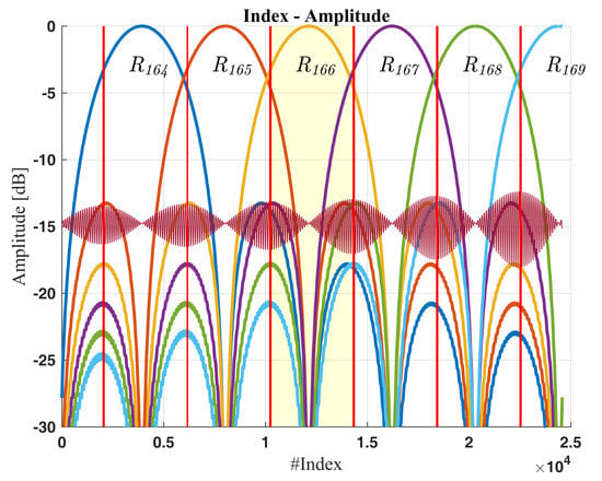
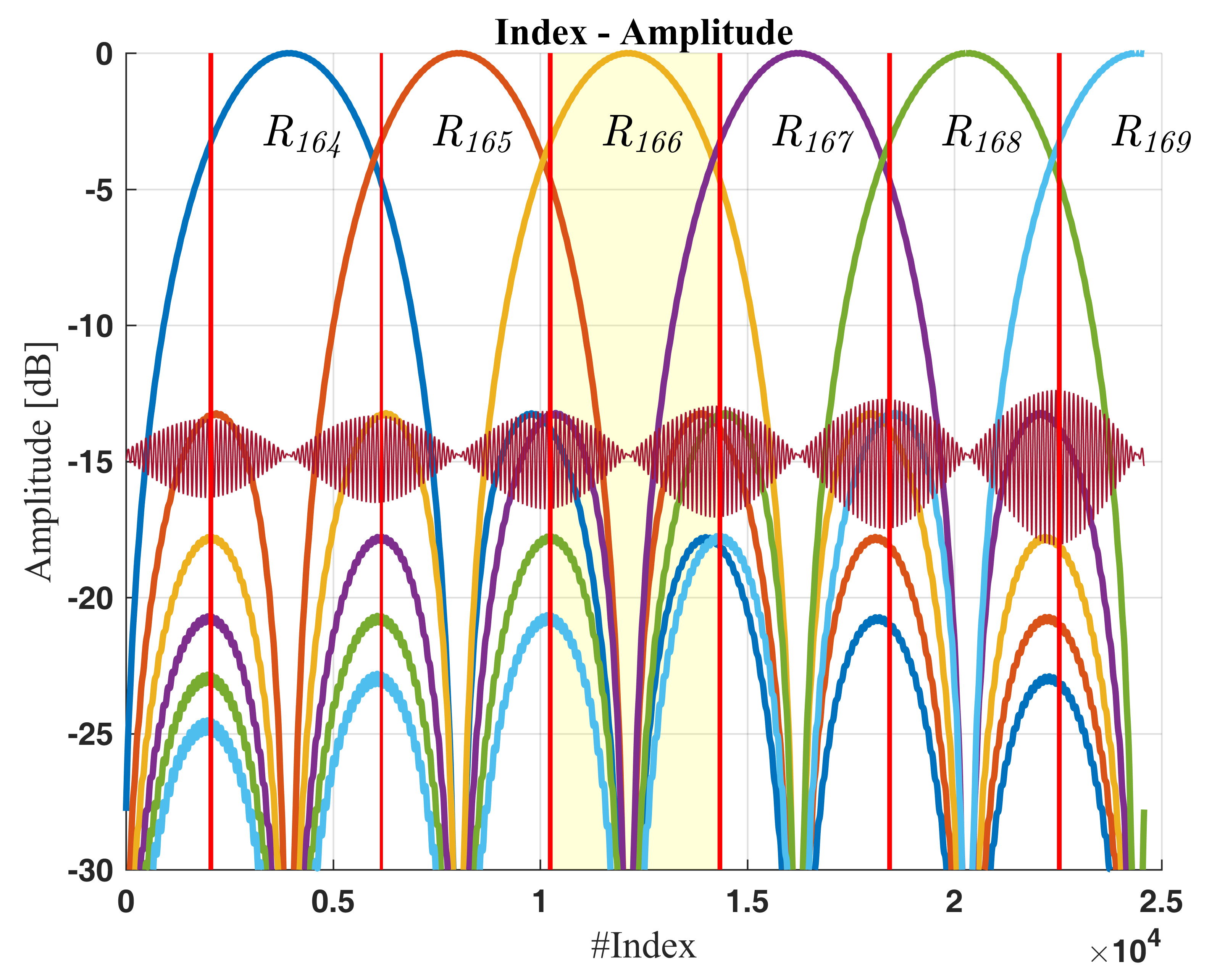
Figure 5a shows how the amplitude of the reflected energy from the towed reflector changes as it is moved away from the radar. The reflector starts in range index 164 and ends in range index 169. The reference reflector remains stationary in range index 177. The amplitude of the stationary reflector is approximately five times lower than the towed reflector due to its smaller size; see Table 1. Figure 5b shows the computed backscatter from the numerical model.

Figure 6a,b shows a cut through Figure 5a,b following the maximum amplitude of the backscattered energy.

The measurements and the computed results correlate to some extent, but major differences are observed, like the reduction in amplitude as the towed reflector is moved away from the radar. The theoretical attenuation from the FSPL, see Equation (16), is approximately 0.33 dB while we observe a close to 3 dB attenuation. This missing 2.7 dB is, as discussed in the next section, believed to be caused by ground reflection or multipath interference. Another difference is the amplitude level of the stationary reflector, which starts 7 dB below the theoretic value and drops in amplitude as the towed reflector gets closer. This is partly believed to be caused by shadowing which will be addressed in Appendix A. The oscillations in the amplitude of the backscatter from the reference reflector are observed in both Figure 6a,b. This oscillation is believed to be caused by constructive and destructive interference between the two reflectors which is discussed in Section 4.3.

4.2. Multipath Interference

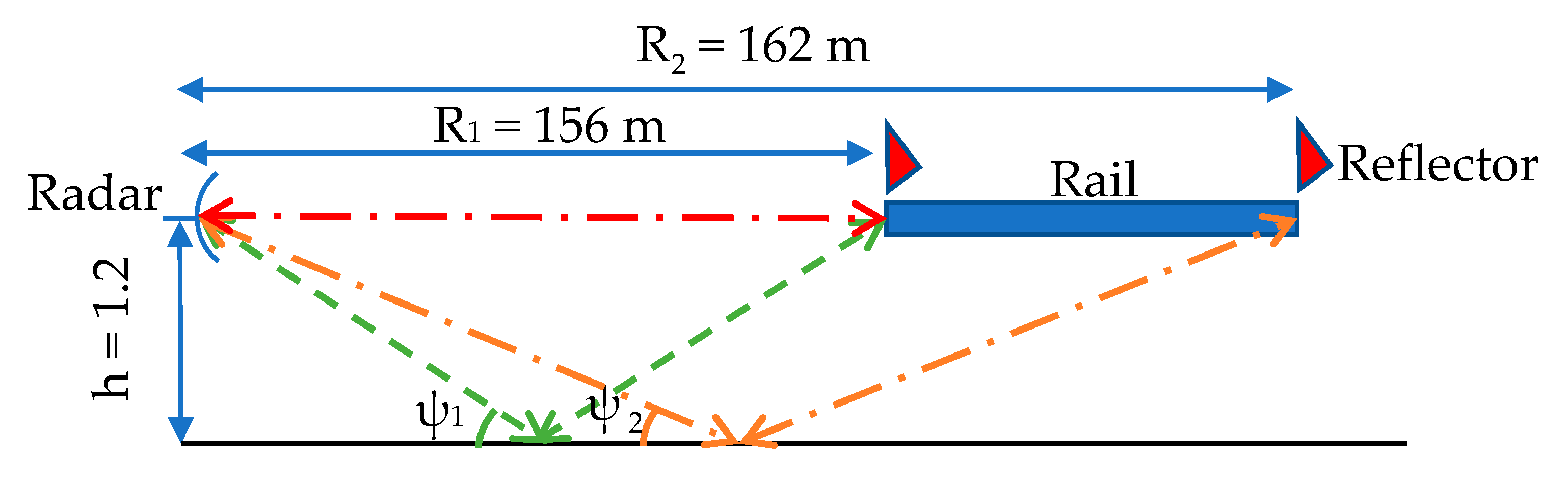
To assess whether the excess damping of the amplitude of the towed reflector was caused by multipath interference, the geometry of the measurement setup was analyzed. During the measurements, the ground was covered by windswept compact snow, which provided a smooth reflecting surface. The difference between the direct path and the indirect path of the backscatter varies with the grazing angle ${\mathsf{\psi }}_{\mathrm{g}}$. In the measurements, the change in grazing angle comes from the towing of the reflector as illustrated in Figure 7.

The geometrical change in range and angle, when towing the reflector, will produce an alternating constructive and destructive pattern according to Equation (13). This pattern is proportional to the wavelength and is inversely proportional to the height of the radar above the ground. In this measurement setup, the first four maxima will occur for a grazing angle of ψ = 0.63°, 1.89°, 3.15°, and 4.41° likewise the four first minima will occur at ψ = 0°, 1.26°, 2.52°, and 3.78°. 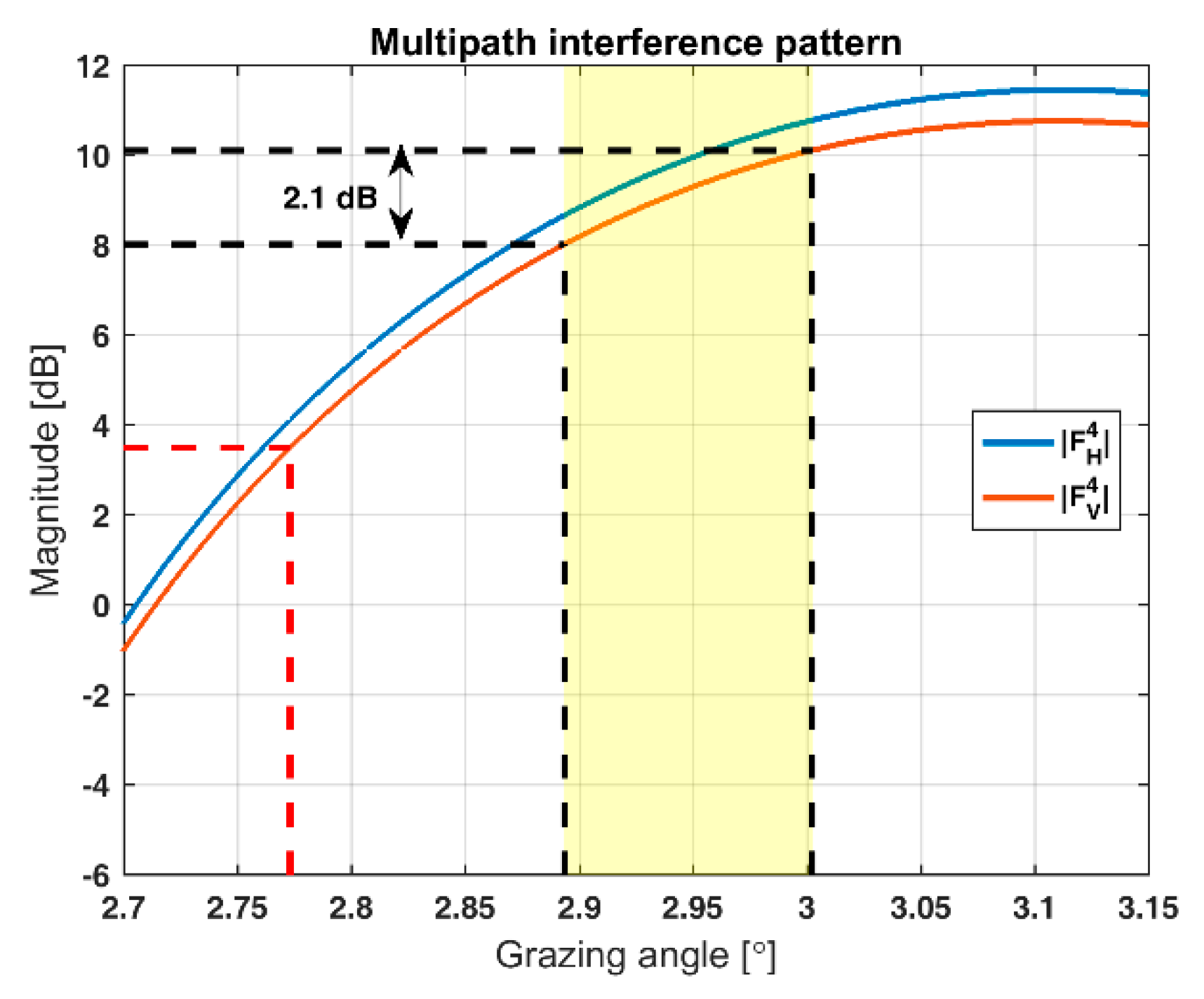Figure 8 shows the variation in amplitude as a function of the grazing angle relevant for the measurement geometry.

Figure 8 shows that a 2.1 dB attenuation of the backscattered energy from the towed reflector due to the change in measurement geometry. By adding the multipath interference loss to the FSPL of 0.3 dB, the total loss is 2.4 dB, which correlates well with the measured 2.7 dB attenuation of the towed reflector. Based on this analysis it is believed that multipath interference is the main cause of the damping of the reflected energy from the towed reflector.

4.3. Constructive and Destructive Interference between Reflectors in the Measurement Scene

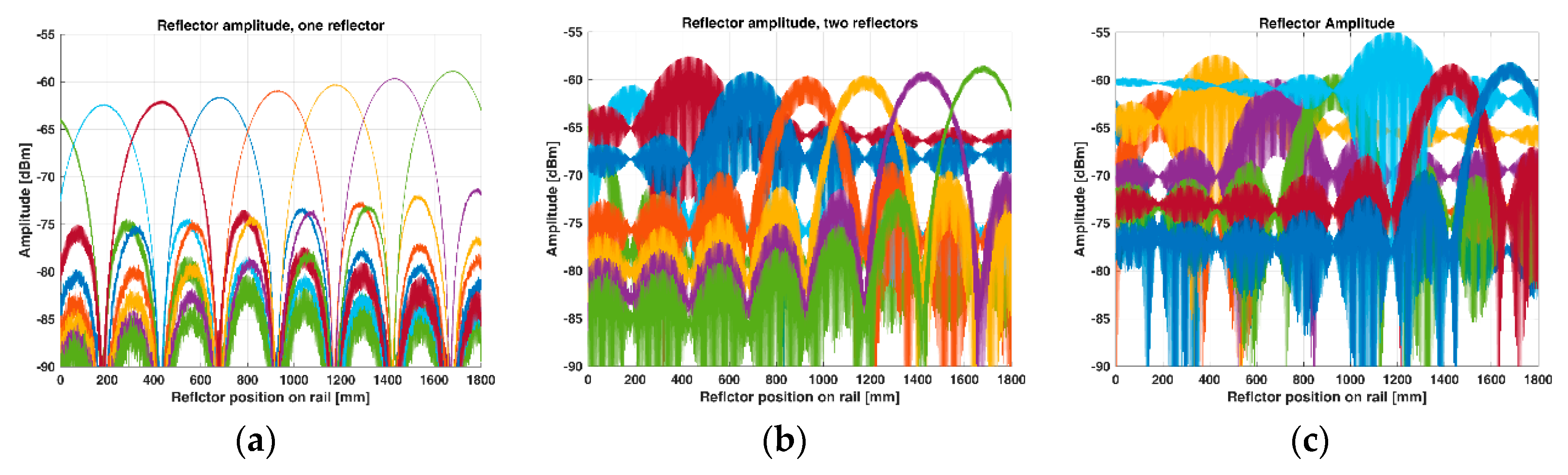
The amplitude oscillations in the backscatter from the stationary reflector in Figure 6 are believed to be caused by inter-reflector interference. The distance to the stationary reflector is constant, hence the frequency of its demodulated signal is constant. The distance to the towed reflector changes proportionally with the tow-speed and the demodulated signal will produce a time-varying increasing frequency. To verify the inter-reflector interference, a laboratory experiment was undertaken, and the measurements are presented in Figure 9.

Figure 9a shows little variation in amplitude of the backscatter from the towed reflector apart from the 3 dB variation which is a function of the reflector’s position within the range cell and the FSPL attenuation of approximately 2 dB. When a second and third reflector are introduced, as shown in Figure 9b,c, there is a noticeable increase in the amplitude variation of the moved reflector. The amplitude decreases with the distance to the stationary reflector, and the peak occurs when they are in the same range cell. In Figure 9b, the stationary reflector is located 0.4 times the distance from the center of the range cell, while in Figure 9c it is located at the center. Based on this experiment, the amplitude variations observed in Figure 6a are believed to be caused by inter-reflector interference.

4.4. Comparison of Measured and Numerically Calculated Inerferometric and Differentail Interferometric Motion

During the outdoor experiment, the actual position of the towed reflector was not recorded. To find the extent of the range cells, the point where the maximum amplitude has fallen by $\sqrt{2}$ or the 3 dB-point is used. However, since there are several environmental effects affecting the amplitude it was simply recorded when the maximum returned energy was shifted from one range cell to the next. 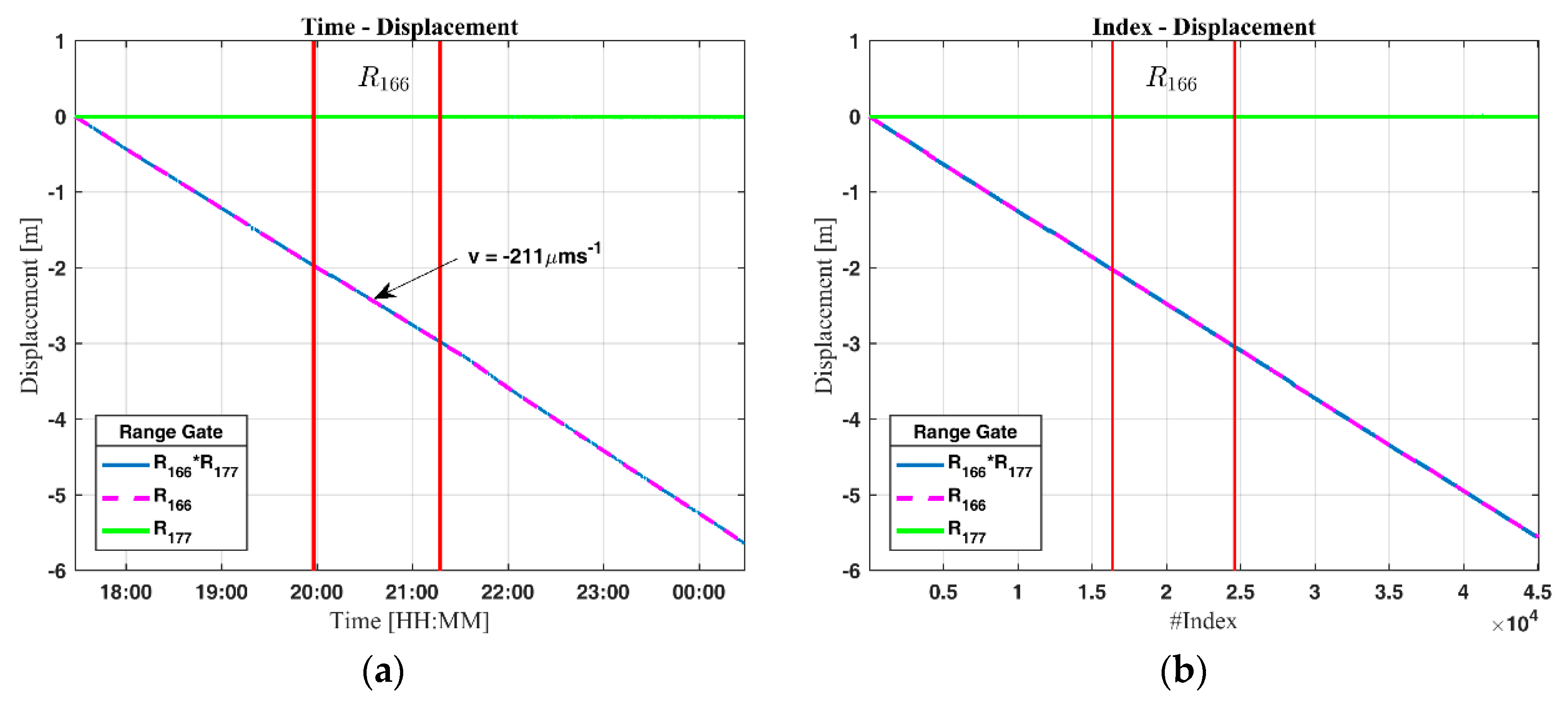The distance between the two amplitude intersections is the range cell resolution, as indicated by the vertical red lines in Figure 6. The measured motion from the outdoor measurement is shown in Figure 10a and the computed motion is show in Figure 10b.

Figure 10a shows the measured displacement of the towed reflector, and Figure 10b shows the computed displacement. As expected, the reference reflector remains stationary while the towed reflector shows a displacement of approximately 5.61 m. The calculated velocity of the motion is −211 µm/s, which corresponds well with the theoretical speed of the winch, which is 220 µm/s. 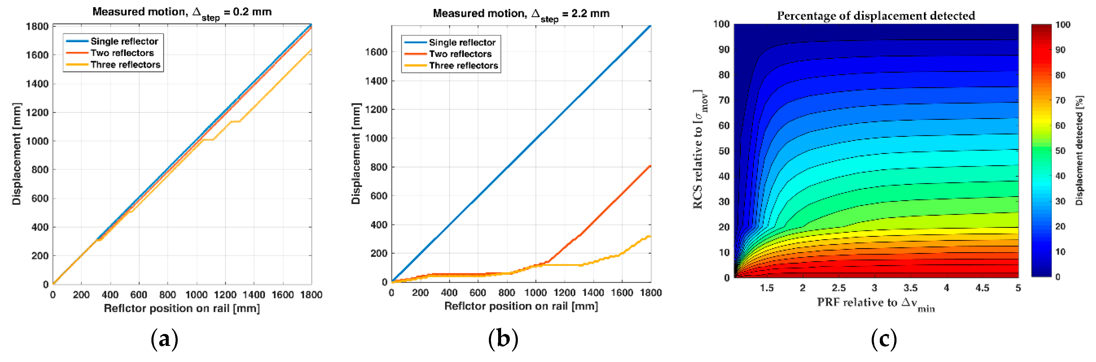The measured displacement from the second laboratory experiment is presented for two different step increments in Figure 11.

Figure 11 shows the measured motion from the three laboratory experiments for two different sampling intervals. In both experiments, the reflector was moved 1800 mm. The blue line shows the single reflector displacement, and the red and yellow lines show the displacement when one and two stationary reflectors are added to the measurement scene. The data is from the same measurement, the only difference is the step-size between the measurements which is equal to a radar setup with three different PRFs. Both measurements fulfill the maximum unambiguous velocity (${\mathrm{V}}_{\max }=0.25\mathsf{\lambda }·\mathrm{PRF}$) as can be seen from the single-reflector displacement (the blue line in Figure 11a,b). When stationary reflectors are introduced, the displacement is partly masked. Figure 11c shows the result of a simulation where a reflector is moved past a stationary reflector. The RCS of the stationary reflector is varied from 0 to 100 times the RCS of the moved reflector, and the PRF is varied from λ/4 to λ/20. The total motion is collected in 20 range cells from the stationary reflector, and the displacement is presented as a percent of the total motion.

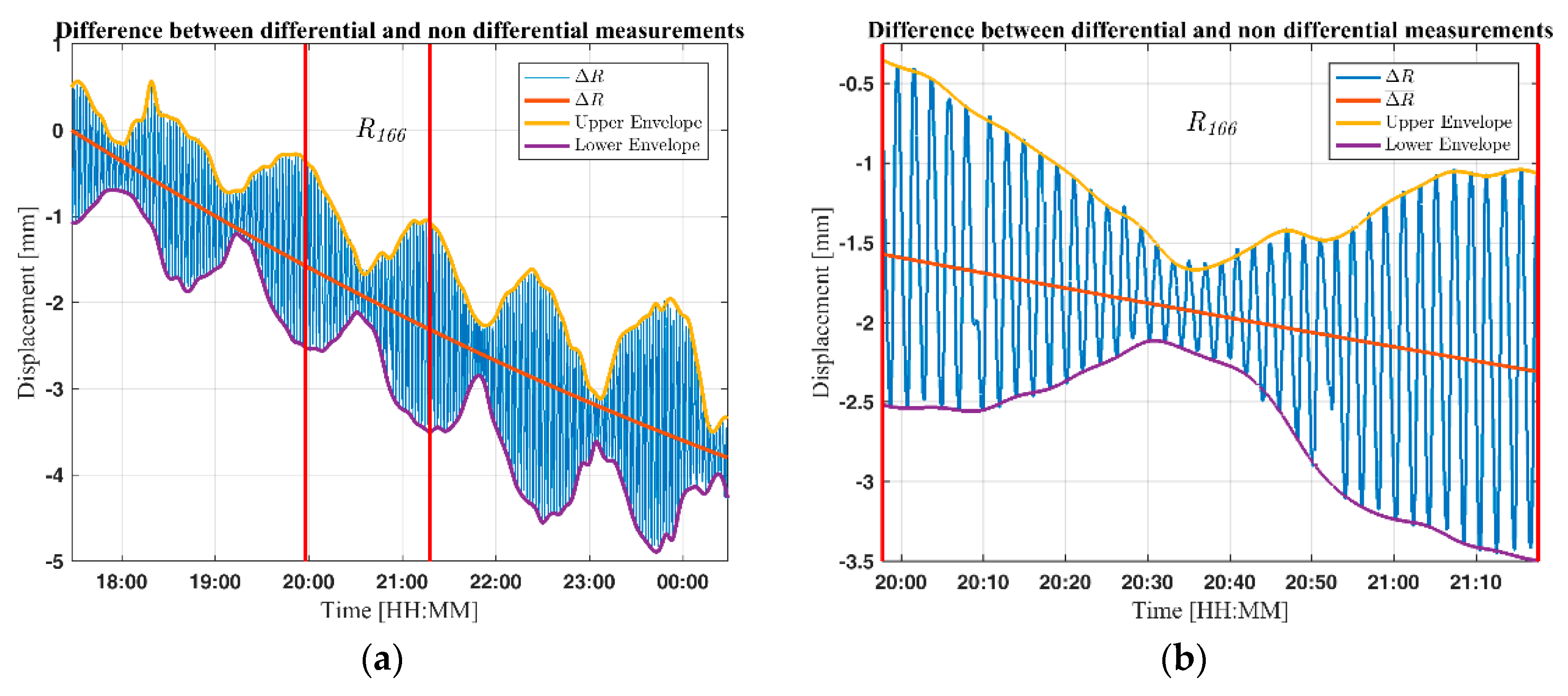
In Figure 12, the determined displacements from the outdoor experiment based on interferometric and differential interferometric measurements are compared.

Figure 12a highlights the difference between the interferometric and differential interferometric measured displacement. Most noticeable are the oscillations in the differential measurements, which reach an amplitude of approximately ±1.5 mm, this oscillation is due to inter-reflector interference. The difference between the two methods is approximately 3.9 mm, which corresponds to 0.7‰ of the total motion. Figure 12b highlights the oscillations in the differential displacement for range index 166. The number of wavelengths per range cell corresponds to the range resolution divided by the wavelength, see Equation (13), which in this setup is 38 wavelengths per range cell.

4.5. Geometric, Environmental and Hardware Influence on Interferometric and Differential Interferometric Measurements

In this section, we assess the deviations in the interferometric and differential interferometric displacements. We analyze the effect the environment, measurement geometry and radar hardware have on the measurement accuracy.

4.6. Radio Refractivity

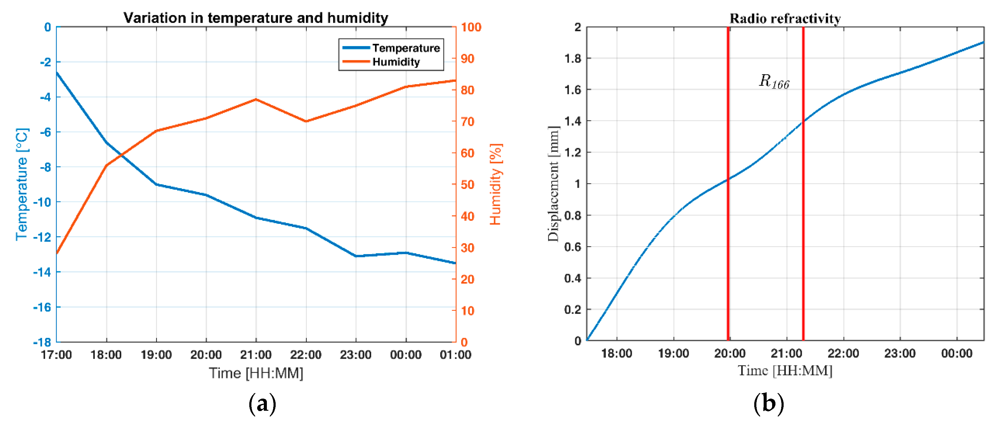
To compensate for the variations in the radio refractivity, an empirical model based on temperature, humidity and pressure may be used ([33]; p. 304). To compensate for atmospheric decorrelation, metrological data was downloaded from the Norwegian Metrological Institutes Station in Ås, located 2.7 km from the measurement site. During the measurements, the temperature dropped from −1.9 °C at 17:00 to −13.1 °C at 01:00 at the same time the relative air humidity increased from 26 to 81%, see Figure 13a. The pressure was not recorded but the mean air pressure was 990 mbar. This gives a change in the refractivity index from n = 298 to n = 314 resulting in an apparent motion of approximately 1.9 mm, see Figure 13b.

By adjusting the displacement for the estimated variation in refractivity the deviation is reduced by 1.9 mm. This is an improvement of nearly 50%, even when the metrological data is not acquired locally.

4.7. Multipath Interference

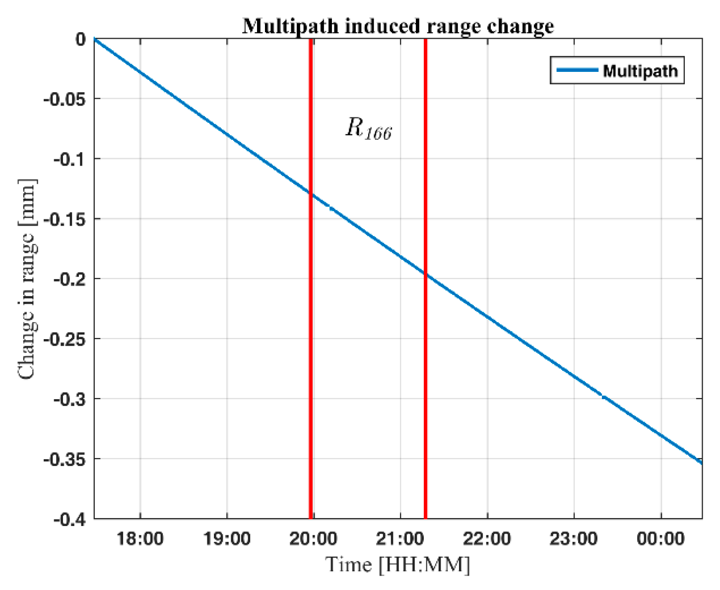
In Section 4.2, multipath interference was found to affect the amplitude of the backscatter from the reflectors. Multipath interference will also affect the phase of the received signal as shown in Figure 14.

The change in distance due to multipath interference during the measurement is estimated to be 0.35 mm.

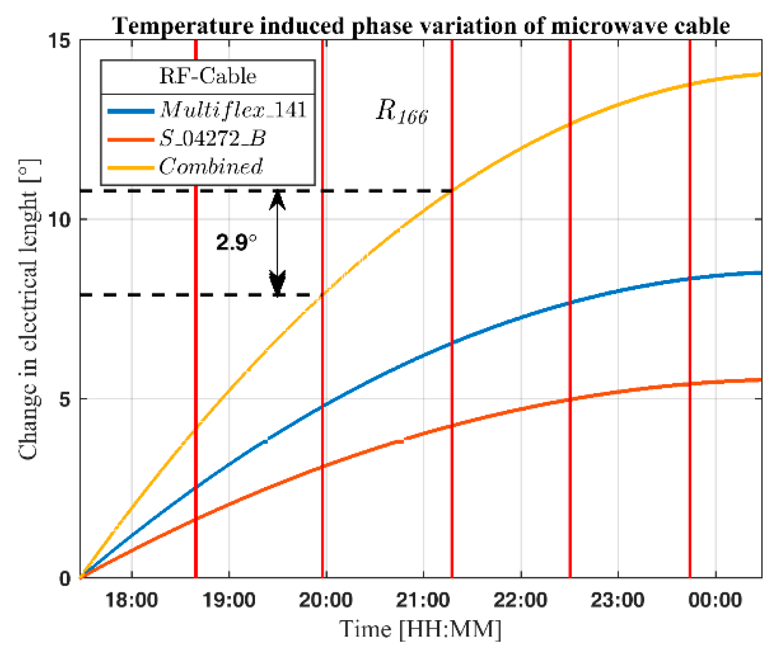
4.8. Electrical Length of the Microwave Cables and Velocity Factor

Varying temperature and/or any change in the path of the electromagnetic waves will affect the accuracy of high precision radar measurements. Two types of microwave cables were used, Huber & Suhner Multiflex_141 and S_04272_B. The total length of the cables was 10.5 m, 4.5 m of Multiflex_141 and 6 m of S_04272_B. The temperature phase variation used for the two cables is Multiflex_141 = 1500 ppm and S_04272_B = 400 ppm [34]. Estimated change in electrical length of the cables used during the measurement based on the same temperature data as used in Section 4.6 is shown in Figure 15.

Applying the estimated change in electrical length of the microwave cable further reduces the difference by approximately 2 mm.

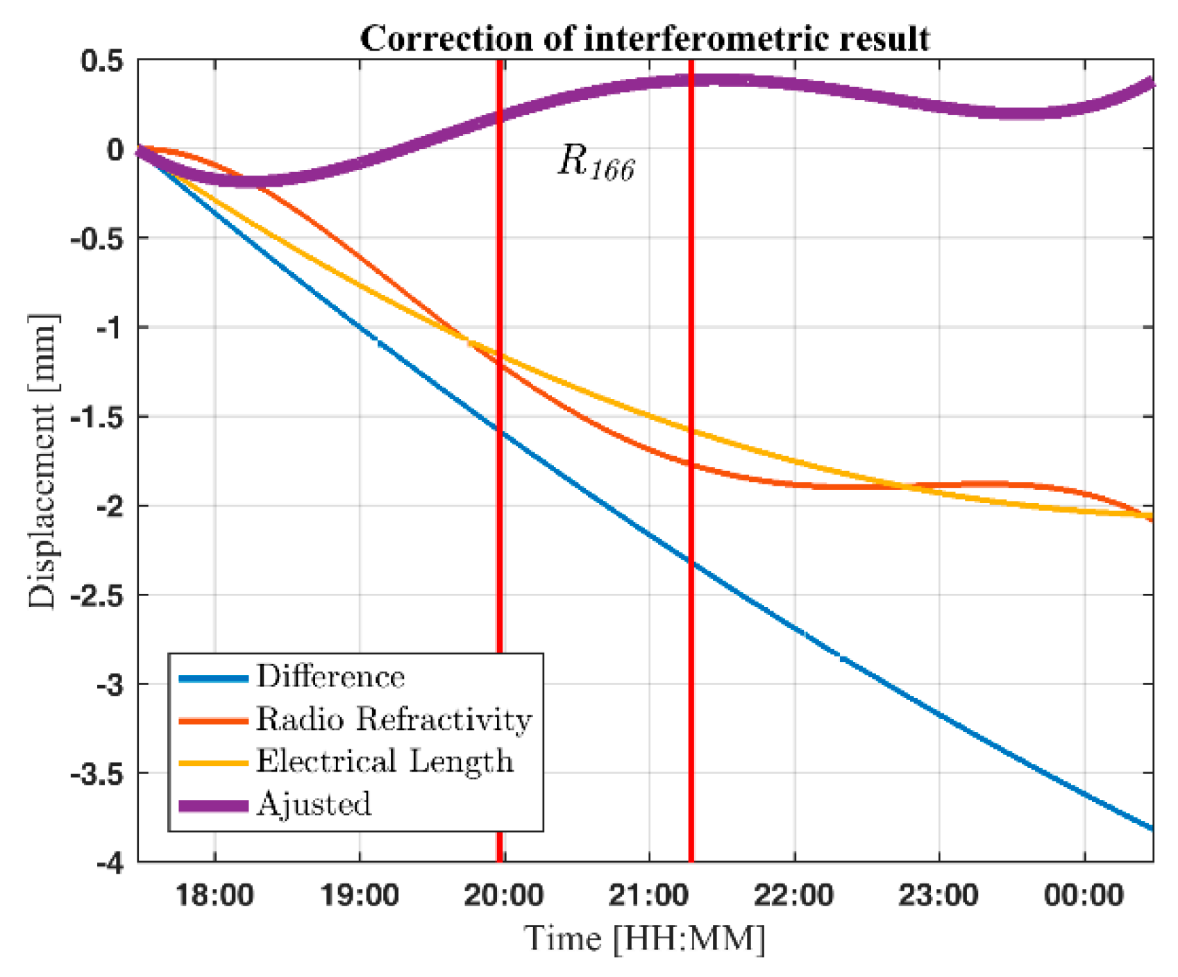
4.9. Result of Compensation

Figure 16 sums up the combined effect of radio refractivity and change in electrical length of the microwave cable. To avoid the effect of inter-reflector interference, the moving mean of the differential displacement is used for comparison.

In Figure 16 the blue line is the difference between the mean differential displacement and the interferometric displacement. The red line is the estimated displacement due to variation in the radio refractivity, the yellow line is the variation in distance due to the change in electrical length of the microwave cables, and the purple line shows the resulting interferometric displacement when the corrections are applied.

4.10. Summary of the Interferometric Experiment

Table 3. Measured and adjusted displacement per range cell in mm. The four center range cells where the motion covers the full extent of the range-cell are marked with gray color.

Range [m]	157	158	159	160	161	162	Sum all range-cells	Sum R158 to R161
Range-index [#]	164	165	166	167	168	169
Interferometry	927.17	1008.20	1005.94	1007.71	1007.38	602.37	5558.8	4029.23
Differential Interferometry	927.30	1007.87	1005.63	1006.98	1006.61	600.43	5554.8	4027.09
Measurement Geometry	1.96	1.94	1.93	1.91	1.89	1.88	11.51	7.67
Radio Refraction	0.10	0.15	0.25	0.37	0.38	0.65	1.90	1.15
Multipath Interference	0.036	0.061	0.061	0.067	0.067	0.062	0.35	0.26
Shadowing	3.87	3.85	3.87	3.48	3.02	2.47	20.57	14.23
Electrical Change in Cable Length	0.61	0.54	0.42	0.27	0.16	0.04	2.05	1.40
Adjusted Interferometry	-	1005.51	1003.28	1005.10	1004.89	-	-	4018.78
Adjusted Differential Interferometry	-	1002.07	999.75	1001.30	1001.43	-	-	4004.52

summarizes geometrical, environmental and electrical effects on the measurement accuracy.

Note that the change in electrical length of the microwave cable only applies to the interferometric computation while shadowing only applies to the differential interferometry. The radio refractivity applies to all computations but for the differential interferometry only by a fraction varying from ¹³/₁₅₇ to ⁷/₁₆₂. Multipath interference and the measurement geometry applies to both methods. The average range cell length measured is 1004.69 mm for interferometry and 1001.13 mm for differential interferometry.

5. Discussion

The experiment shows that the accuracy of both interferometry and differential interferometry depends on the measurement geometry, variations in radio refractivity, multipath interference, interference between scatterers, and the radar hardware. In this chapter, the influence of these effects are discussed. The discussion is divided into three sections: Amplitude, phase and radar hardware. Some general advice is then given on how to minimize the impact of these effects in an operational system.

5.1. Amplitude

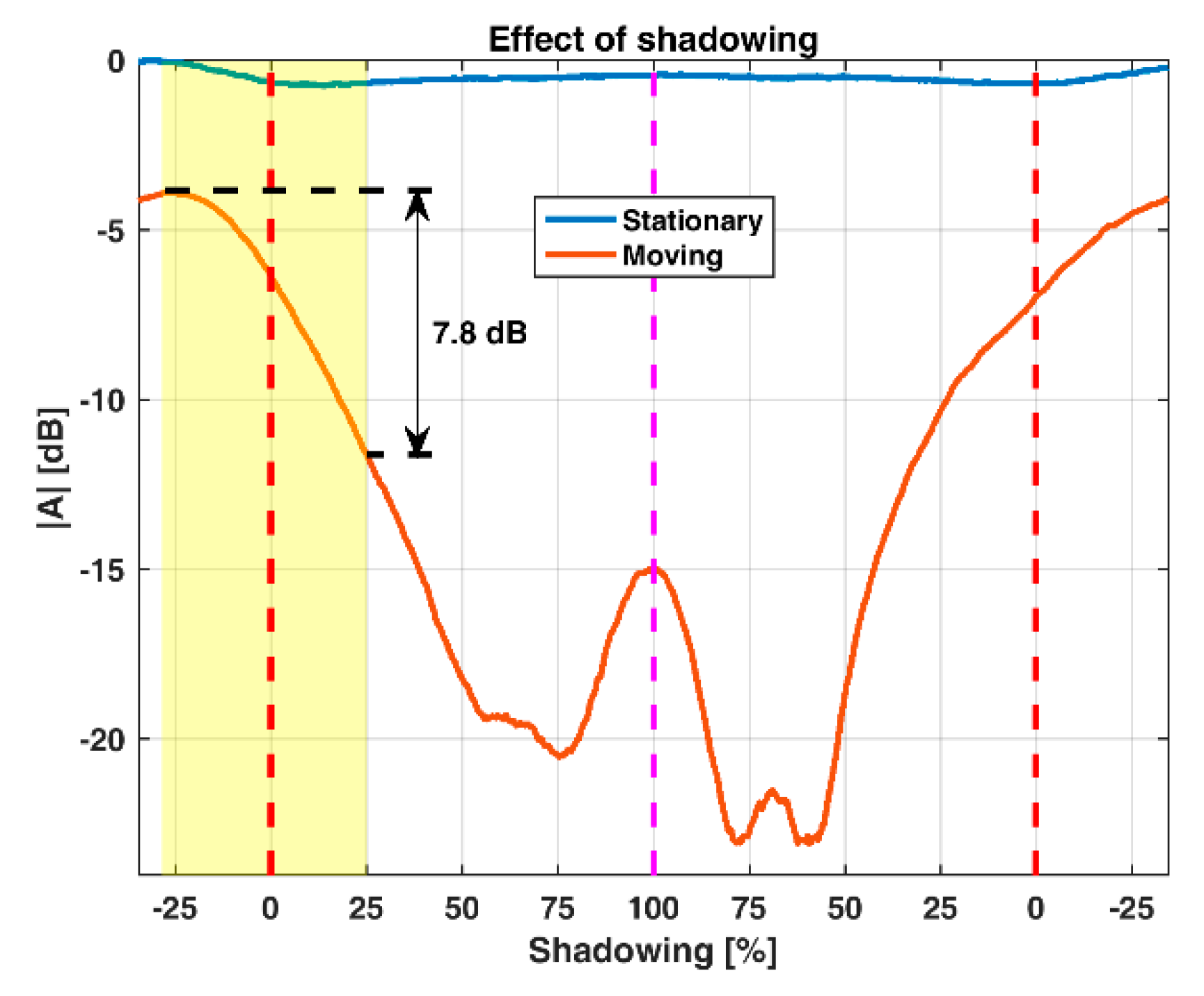
The amplitude data is often the first information to assess when analyzing radar measurements. Any deviations in backscattered energy from reflectors compared to what is expected from theoretical values are easily detectable. Two effects were observed, damping and oscillations. The theoretical RCS of the towed reflector is 20.4 dBsm and the theoretical RCS of the stationary reflector is 13.1 dBsm. This gives a difference in backscatter between the two reflectors of 7.3 dB, while the measured difference was approximately 21.7 dB when the towed reflector was at the far end of the rail. Three major effects may explain this difference: Multipath interference, shadowing (for details see Appendix A) and propagation loss. First, the multipath interference-induced gain of the towed reflector, which is estimated to 8 dB when the towed reflector is at the end of the rail, and the multipath interference-induced gain of the stationary reflector, which is estimated to be 3.5 dB, see Figure 8. This gives a 4.5 dB multipath interference gain. Second, the contribution from shadowing which is estimated to be 7.8 dB (see Appendix A). Third, the FSPL that is 0.7 dB. The combined total of these three effects are 13 dB. Subtracting the combined contribution from the measured value gives a difference of 8.9 dB, which agrees with the theoretical difference of 7.3 dB. The deviation of 1.6 dB might come from using uncalibrated corner reflectors, by misalignment of one or both reflectors, and inaccurate measuring of reflector and radar antenna height. The results show that the combined effect of measurement geometry, multipath interference and shadowing may give large time variations in the backscattered energy from scatterers in the measurement scene. In a measurement scene with many moving scatterers, tracking of natural scatterers can be challenging as they may disappear and reappear depending on geometry, shadowing and motion.

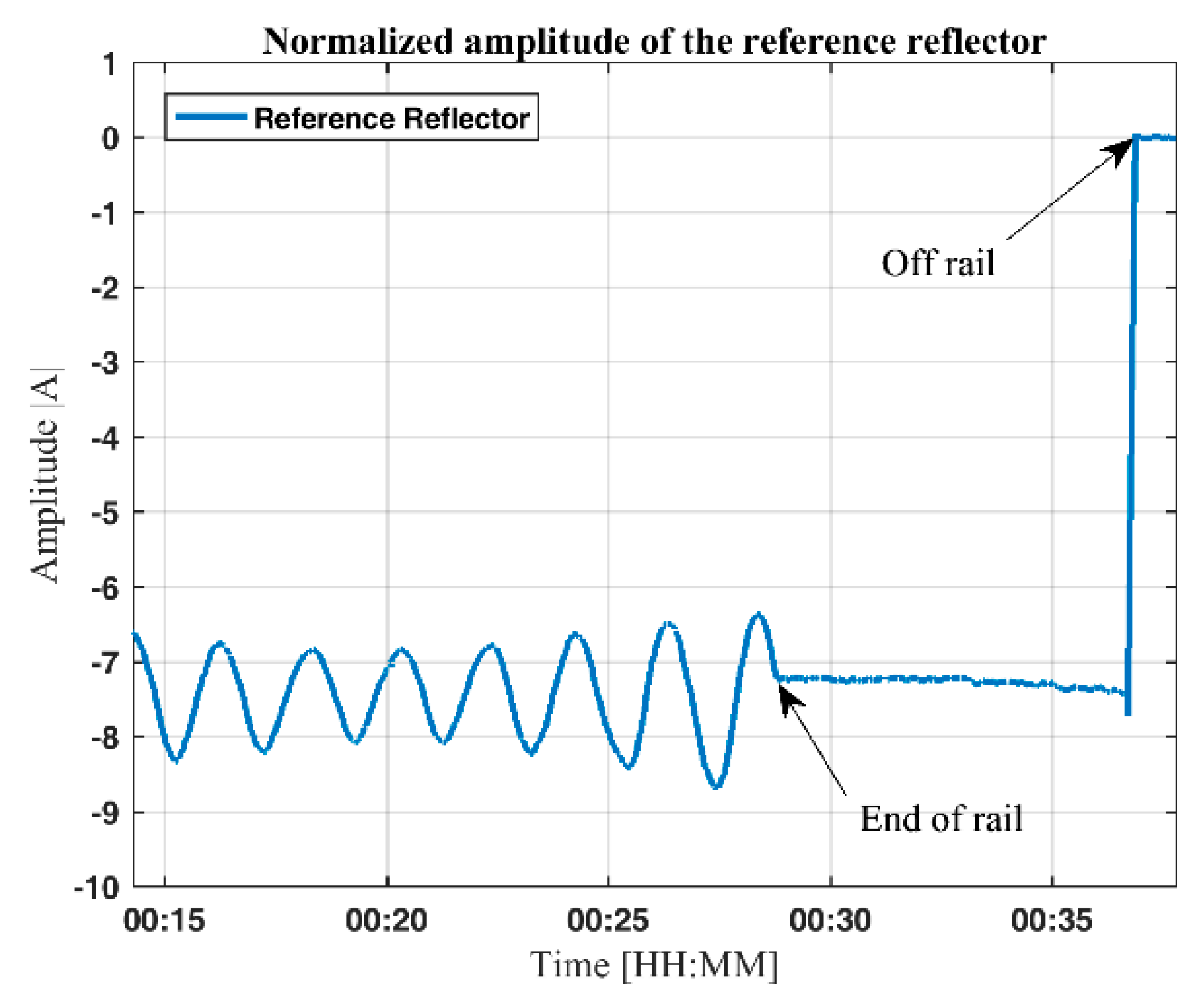
The shadowing of the stationary reflector was found to be the main cause of the damping of the reflected energy. This is supported both by observing the increase in reflected energy backscattered from the reference reflector as the towed reflector was towed beyond the end of the rail, see Figure A1, and by the reflector shadowing experiment in the laboratory, see Figure A3.

The oscillations observed in the amplitude of the backscatter from the reference reflector are caused by inter-reflector interference between the two reflectors in the measurement scene. The oscillation increase as the towed reflector gets closer to the stationary reflector, see Figure 9a. The interference is visible in both Figure 9a,b, however, the amplitude of the oscillations is higher for the stationary reflector than for the towed reflector. This is due to the mutual size difference, i.e., the largest reflector has a greater influence on the small reflector than the small reflector on the large reflector. Maximum constructive interference between two reflectors occurs when the mutual distance, ΔR, is equal to integer multiples of the wavelength of the transmitted signal and maximum destructive interference that occurs when the mutual distance is equal to integer multiples of half the wavelength. The amplitude of the interference will follow a sine cardinal pattern due to the Fourier transform when going from the time domain to frequency domain. The maximum and minimum amplitude will occur when the two reflectors are in the same range cell, see Figure 9. This shows that all scatterers within the measurement scene may affect each other and the magnitude of the interference depends on the reflected energy of the scatterers according to the exponent in Equation (13).

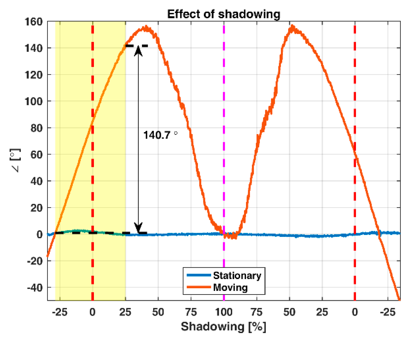
5.2. Phase

As discussed in the previous section, the effect of radio refractivity, multipath interference, inter-reflector interference, and shadowing affects the amplitude. In addition, it affects the phase of the reflections, see Figure 13, Figure 14 and Figure 15.

The variation in radio refractivity during the measurements was estimated based on meteorological data and was found to contribute to almost 50% of the deviation between the interferometric and the differential interferometric displacement. The temporal sampling rate of the meteorological data was 1 h. This gives a relatively large uncertainty in the computations. Another factor adding to the uncertainty is the distance between the radar site and the meteorological station that is 2.7 km. However, we show that the corrections of radio refractivity improve the results. The influence of the variation in radio refractivity increases with distance; hence, in real-life setups the contribution may be substantially higher.

The effect of multipath interference depends on the geometry of the measurement setup and since the height of the antennas and reflectors were recorded manually, a fair amount of tolerance in the result is to be expected. The change of 0.35 mm for the 6 m tow of the reflector in this setup might seem to be insignificant, but given another setup geometry, the effect might be significantly higher. The effect of multipath interference should therefore always be considered as a source of measurement error in high-precision measurements. The estimation of multipath interference is a challenging task in real-life measurements due to temporal variation in the reflection coefficient as the backscatter depends on surface roughness, moisture and texture [35].

The effect of shadowing was, based on the laboratory measurements, found to contribute to 14.2 mm of the measured displacement of the differential result. The laboratory experiment was based on the measured geometry of the field experiment and some uncertainty is expected in the result. The effect of shadowing was an unintended result of an unfortunate measurement setup and is only added to explain the measured deviations. In some remote sensing scenarios, shadowing might be unavoidable, leading to low coherence and consequently, could be detrimental for the monitoring [24].

The laboratory experiment shows that inter-reflector interference can mask the motion. To avoid this, the backscatter of the moving object should be higher than the backscatter of the stationary object, see Figure 11c. This follows directly from Equation (13), which states that the energy backscatter of a range cell is the coherent sum of all the scatterers within the range cell. In GB-SAR, this applies both in the down and cross range [24] (Figure 7b). This result indicates that it is beneficial to introduce reflectors to the measurement scene to follow the motion of point objects. The introduction of a reflector is artificial, but it can be viewed without loss of generality as natural stationary clutter or infrastructure like rockfall catch fences in a real-life measurement scene either in the mainlobe or in the sidelobe. This indicated that in a measurement scene without a distinct scatterer, care should be exercised when analyzing the displacement.

The variation in radio refractivity applies to both interferometry and differential interferometry, but for differential interferometry only by a fraction equal to the length between the reflectors. The multipath interference applies to both interferometry and differential interferometry.

5.3. Radar Hardware

A part of the difference between the interferometric and differential interferometric results may be explained by variations in the radar hardware. If the variations due to the radar hardware can be measured or predicted, the measurements can be corrected. The main source affecting the modulation bandwidth is the accuracy of the reference clock of the signal generator. Inside the radar used during this experiment there are two oscillators, one for the local oscillator, one for the sweep generator (DDS). Fluctuations in any of these oscillators will affect the measurements. The total uncertainty of the DDS reference oscillator is used in the GB-InRAR ±23 ppm, disregarding any aging effects. This may lead to variations in the transmitted bandwidth. Due to programming technicalities, the effective bandwidth from the DDS multiplier chain was 149,912,000 MHz. This will give a maximum decrease in range cell length by approximately 0.6 mm, giving a total of 3.5 mm for the 6 m tow of the reflector further reducing the deviation between the measured and computed movement. This effect is independent of distance and applies to all range cells.

The temperature-induced change in electrical length of the microwave cables contributed to a variation in range, which is visible in the measurements. The total effect of this change was approximately 2 mm. This estimate is based on meteorological data from a station 2.7 km away from the radar, leading to uncertainties in the calculations. The estimated change in electrical length of the microwave cables are based on coarse values from data sheets; a fair amount of tolerance in the calculations are expected. The temperature–phase relationship of a microwave cable is complex, and it is usually measured and not numerically modelled. To minimize error, the microwave cables used should be temperature cycled to get the correct temperature–phase variation.

5.4. Measured Displacement

The measured difference in displacement between interferometry and the mean differential motion is approximately 3.9 mm, see Figure 12a. The mean displacement was used for the differential interferometric displacement to avoid the inter-reflector interference to influence the interferometric result. The average range cell size was estimated to be 1007.3 mm for interferometry and 1006.8 mm for differential interferometry. After adjusting the interferometric displacement for measurement geometry, variation in radio refractivity, multipath interference, change in electric length of the microwave cable, and actual bandwidth, the average range-cell size was reduced to 1004.1 mm. The differential displacement was adjusted for measurement geometry, multipath interference, shadowing, and actual bandwidth, resulting in an average range cell size of 1000.5 mm. The major part of the difference between the two methods are believed to come from inaccuracy in the data used to calculate the variation in radio refractivity and change in electric length of the microwave cable as the temperature and humidity data was not recorded locally. There is some measurement uncertainty with the geometry of the measurement setup, but this will affect both methods equally except for the shadowing, which only applies to the differential method.

The differential displacement is closer to the theoretical range cell length of 1 m, but this is the mean motion. The inter-reflector interference displayed in Figure 12a shows a range variation of approximately ±1.5 mm, which is a product of the measurement setup and not a physical motion. This effect will diminish by increasing the distance between the reflectors, but care should be exercised when placing a reference reflector.

5.5. Minimizing the Influence of Geometic, Environmental, and Radar Hardware Effects in Operational Monitoring

In this section, we summarize the findings and give general advice on how to avoid or reduce the impact of the effects presented in this chapter.

The impact of radio refractivity is frequency dependent and it is stated in Reference [14] that the longest radar waves possible should be used to minimize the effect of atmospheric variations. Using a lower frequency has the inherent consequence of a larger antenna to achieve the same beamwidth as the beamwidth is approximately given as λ/L, where L is the physical size of the antenna ([22]; p. 6.8). Applying meteorological data collected locally has been shown in a number of studies to be an efficient way to compensate for atmospheric decorrelation [8,13,17,18,19,20].

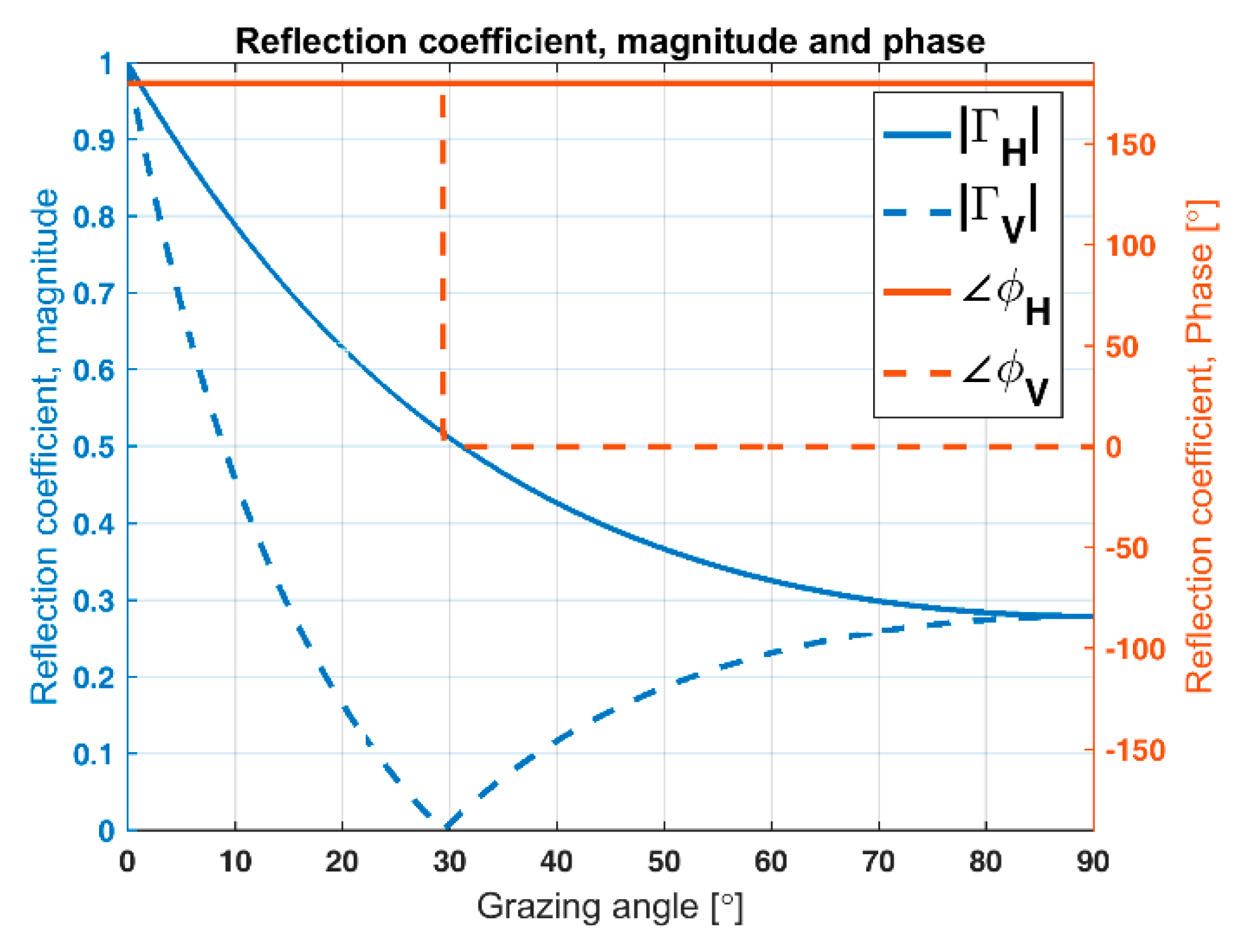
To minimize the effect of multipath interference, the vertical part of the antenna lobe should not illuminate the ground. This can be controlled by adjusting the elevation angle of the antenna and by using an antenna with a narrow elevation beam. If the installation geometry prohibits this, vertical polarization is preferable as it generates less multipath interference than horizontal polarization. This can be seen from Figure 1 where the magnitude of the reflection coefficient for VV-polarization is significantly lower than for HH-polarization. Hence, multipath interference is less at VV-polarization than at HH-polarization. This was also one of the main findings in Reference [21]. Another way of reducing multipath interference is by adding shielding of the antennas, preventing the radar waves from illuminating the reflective surface as presented in Reference [21]. They state in their experiment that this greatly reduced the problem, but it did not eliminate the interference. They also recommend installing the radar at an elevated area if possible. If none of the above measures is possible, this study has shown that the effect of multipath interference can be reduced by applying corrections based on analysis of the measurement geometry and the reflective surface.

Unless the backscatter from the object or surface in motion is stronger than the backscatter from the surroundings, inter-reflector interference can mask the motion as shown in Figure 11. One way to avoid this effect is by introducing an artificial reflector. The laboratory experiment also showed that a high PRF partly helps to resolve the problem. Both the outdoor and laboratory experiments showed that the interference between strong reflections where one object is in motion results in oscillations in the amplitude of the backscatter. This indicated that care should be taken when measuring objects in strong clutter, so that the motion of the monitored object or area is not suppressed by backscatter from stationary clutter. The general solution is to use a large antenna with a narrow beam to reduce the illuminated area and reduce the range cell size i.e., use a wideband radar.

The reference oscillator should be of high quality and preferably both temperature and voltage compensated.

The temperature-induced phase shift in the microwave cables may be reduced by keeping the cables as short as possible and by using high performance cables with low a temperature–phase coefficient. In Reference [23] it is suggested to use active temperature stabilization of the cables to minimize the phase–temperature variation. They also recommend using PTFE-free cables for operating temperatures below 22 °C. One solution to monitor the major variations in phase due to radar hardware is to measure the phase of the antenna cross-talk and to adjust the measurements accordingly.

6. Conclusions

A GB-InRAR system is used for experimental interferometric and differential interferometric measurement experiments in the field and laboratory with a moving trihedral corner reflector. A theoretical model is developed to asses measurement uncertainties for the geometry of the measurement setup, atmospheric effects i.e., radio refractivity and the effect of ground reflections i.e., multipath interference, radar target interference and the radar hardware.

It is shown that major deviations between interferometric and differential interferometric calculated displacement can be explained by variations in environmental and geometrical effects. The accuracy of interferometry can be comparable to the differential accuracy when adjusted for environmental variations. For the analyzed experiment, the major contributing environmental effects are radio refractivity and temperature-induced change in electrical length of the microwave cables. The major geometrical effects are multipath interference and inter-reflector interference.

The experiments show inter-reflector interference, which for the differential method resulted in oscillations in measured displacement. The amplitude of these oscillations increased inversely with distance peaking when they were in the same range cell. It is shown that the motion can be masked when the backscatter from the stationary object is equal or higher than the backscatter from the moving object. It was also shown that the effect of inter-reflector interference could be reduced by using a high PRF.

The accuracy of both methods can be improved by adjusting for offsets in the radar hardware. The temperature-induced change in the electrical length of the microwave cables can be significant, and it should be considered separately to avoid mixing the effect with the radio refractivity, which is also influenced by variation in temperature.

The results derived from the experiment verify that the GB-InRAR can detect and monitor small displacements. The analysis suggests that differential interferometry is close to unaffected by radio refractivity but vulnerable to inter-reflector interference.

The compensated average interferometric displacement is within 4‰ of the theoretical range cell size while the compensated average differential displacement is within 1‰ of the theoretical range cell size. Validation of the experiments is based on general radar theory, and the calculations and results should be valid for other radar systems.

References

1. Mecatti, D.; Macaluso, G.; Barucci, A.; Noferini, L.; Pieraccini, M.; Atzeni, C. Monitoring open-pit quarries by interferometric radar for safety purposes. In Proceedings of the 7th European Radar Conference, Paris, France, 30 September–1 October 2010. [Google Scholar]
2. Di Pasquale, A.; Nico, G.; Pitullo, A.; Prezioso, G. Monitoring strategies of earth dams by ground-based radar interferometry: How to extract useful information for seismic risk assessment. Sensors 2018, 18, 244. [Google Scholar] [CrossRef] [PubMed]
3. Lukin, K.; Anatoliy, M.; Palamarchuk, V.P.; Vyplavin, P.L.; Kozhan, E.; Lukin, S. Monitoring of St. Sophia Cathedral interior using Ka-band Ground Based Noise Waveform SAR. In Proceedings of the 2009 European Radar Conference (EuRAD), Rome, Italy, 30 September–2 October 2009; pp. 215–217, ISBN 9781424447473. [Google Scholar]
4. Liu, X.; Lu, Z.; Yang, W.; Huang, M.; Tong, X. Dynamic monitoring and vibration analysis of ancient bridges by ground-based microwave interferometry and the ESMD method. Remote Sens. 2018, 10, 770. [Google Scholar] [CrossRef]
5. Luzi, G.; Crosetto, M.; Fernández, E. Radar interferometry for monitoring the vibration characteristics of buildings and civil structures: Recent case studies in Spain. Sensors 2017, 17, 669. [Google Scholar] [CrossRef] [PubMed]
6. Gundersen, R.; Norland, R.; Denby Rolstad, C. Ground-Based Differential interferometric radar monitoring of unstable mountain blocks in a coastal environment. Remote Sens. 2018, 10, 914. [Google Scholar] [CrossRef]
7. Norland, R. Differential Interferometric Radar for Mountain Rock Slide Hazard Monitoring. In Proceedings of the 2006 IEEE International Symposium on Geoscience and Remote Sensing, Denver, CO, USA, 31 July–4 August 2006; pp. 3293–3296. [Google Scholar] [CrossRef]
8. Norland, R. Improving Interferometric Radar Measurement Accuracy using local Meteorological Data. In Proceedings of the IGARSS 2007 IEEE International Geoscience and Remote Sensing Symposium, Barcelona, Spain, 23–28 July 2007; pp. 3293–3296. [Google Scholar] [CrossRef]
9. Norland, R.; Gundersen, R. Use of radar for landslide hazard monitoring. In Landslides and Avalanches: ICFL 2005 Norway: Proceedings of the 11th International Conference and Field Trip on Landslides, Norway, 1–10 September 2005; Taylor & Francis: London, UK, 2005. [Google Scholar]
10. Luzi, G.; Pieraccini, M.; Mecatti, D.; Noferini, L.; Macaluso, G.; Galaro, A.; Atzeni, C. Advances in ground-based microwave interferometry for landslide survey: A case study. Int. J. Remote Sens. 2006, 27, 2331–2350. [Google Scholar] [CrossRef]
11. Rolstad, C.; Norland, R. Ground-based interferometric radar for velocity and calving-rate measurements of the tidewater glacier at Kronebreen, Svalbard. Ann. Glaciol. 2009, 50, 47–54. [Google Scholar] [CrossRef]
12. Gundersen, R.; Norland, R.; Denby Rolstad, C. Monitoring glacier flow with ground-based interferometric radar in Ny-Ålesund, Svalbard. Polar Res. 2018. under review. [Google Scholar]
13. Luzi, G.; Dematteis, N.; Zucca, F.; Monserrat, O.; Giordan, D.; Lopez Moreno, J. Terrestrial radar interferometry to monitor glaciers with complex atmospheric screen. In Proceedings of the 2018 International Geoscience and Remote Sensing Symposium, Valencia, Spain, 22–27 July 2018; pp. 6243–6246. [Google Scholar]
14. Zebker, H.; Rosen, P.; Hensley, S. Atmospheric effects in interferometric synthetic aperture radar surface deformation and topographic maps. J. Geophys. Res. 1997, 102, 7547–7563. [Google Scholar] [CrossRef] [Green Version]
15. Ferretti, A.; Prati, C.; Rocca, F. Nonlinear Subsidence Rate Estimation Using permanent scatterers in differential SAR interferometry. IEEE Trans. Geosci. Remote Sens. 2000, 38, 2202–2212. [Google Scholar] [CrossRef]
16. Kempes, B. Radar Interferometry, Persistent Scatterer Technique; Springer: Munich, Germany, 2006; ISBN 9781402045769. [Google Scholar]
17. Luzi, G.; Pieraccini, M.; Mecatti, D.; Noferini, L.; Guidi, G.; Moia, F.; Atzeni, C. Ground-based radar interferometry for landslides monitoring: Atmospheric and instrumental decorrelation sources on experimental data. IEEE Trans. Geosci. Remote Sens. 2004, 42, 2454–2466. [Google Scholar] [CrossRef]
18. Noferini, L.; Pieraccini, M.; Mecatti, D.; Luzi, G.; Atzeni, C.; Tamburini, A.; Broccolato, M. Permanent scatterers analysis for atmospheric correction in ground-based SAR interferometry. IEEE Trans. Geosci. Remote Sens. 2005, 43, 1459–1471. [Google Scholar] [CrossRef]
19. Pipia, L.; Fàbregas, X.; Aguasca, A.; López-Martínez, C. Atmospheric artifact compensation in ground-based DInSAR applications. IEEE Geosci. Remote Sens. Lett. 2008, 5, 88–92. [Google Scholar] [CrossRef]
20. Monti Guarnieri, A.; Iannini, L.; Giudici, D. Atmospheric phase screen in ground-based radar: Statistics and compensation. IEEE Geosci. Remote Sens. Lett. 2011, 8, 537–541. [Google Scholar] [CrossRef]
21. Lucas, C.; Leinss, S.; Bühler, Y.; Marino, A.; Hajnsek, I. Multipath interferences in ground-based radar data: A case study. Remote Sens. 2017, 9, 1260. [Google Scholar] [CrossRef]
22. Skolnik, M. (Ed.) Radar Handbook, 2nd ed.; McGraw-Hill Education: Boston, MA, USA, 1990; p. 1200. ISBN 9780070579132. [Google Scholar]
23. Czuba, K.; Sikora, D. Temperature stability of coaxial cables. ACTA Phys. Pol. 2011, 119, 553–557. [Google Scholar] [CrossRef]
24. Frukacz, M.; Wieser, A. On the impact of rockfall catch fences on ground-based radar interferometry. Landslides 2017, 14, 1431–1440. [Google Scholar] [CrossRef] [Green Version]
25. Frukacz, M.; Wieser, A. Terrestrial radar interferometry with objects observed through protection fences. In Proceedings of the 18 Internationaler Ingenieurvermessungskurs Graz, Graz, Austria, 25–29 April 2017. [Google Scholar]
26. Gurgel, K.; Schlick, T. Remarks on Signal Processing in HF Radars Using FMCW Modulation; International Radar Symposium IRS: Hamburg, Germany, 2009. [Google Scholar]
27. Levanon, N. Radar Principles; John Wiley & Sons: Tel-Aviv, Israel, 1988; ISBN 0471858811. [Google Scholar]
28. Stiles, W.; Ulaby, F. Dielectric Properties of Snow; University of Kansas: Lawrence, KS, USA, 1980. [Google Scholar]
29. Frolov, A.D.; Macheret, Y.Y. On dielectric properties of dry and wet snow. Hydrol. Process. 1999, 13, 1755–1760. [Google Scholar] [CrossRef]
30. Mahafza, B.R. Radar Systems & Analysis and Design Using Matlab; Chapman & Hall: Huntsville, AL, USA, 2000; p. 772. ISBN 978-158-488-182-7. [Google Scholar]
31. Pozar, D. Microwave Engineering, 4th ed.; John Wiley & Sons Inc.: Amherst, MA, USA, 2012; p. 732. ISBN 9780470631553. [Google Scholar]
32. ITU. RECOMMENDATION ITU-R P.525-3, Calculation of Free-Space Attenuation; International Telecommunication Union: Geneva, Switzerland, 2016. [Google Scholar]
33. Morchin, W. Radar Engineer’s Sourcebook; Artech House Publisher: Northwood, MA, USA, 1992; p. 496. ISBN 9780890065594. [Google Scholar]
34. Fosli, E.; Bredengen AS, Oslo, Norway. Personal communication, 2018.
35. Ulaby, F.; Batlivala, P.; Dobson, M. Microwave backscatter dependence on surface roughness, soil moisture, and soil texture: Part I-bare soil. IEEE Trans. Geosci. Electron. 1978, 16, 286–295. [Google Scholar] [CrossRef]
Figure 1. The Fresnel reflection coefficient as a function of grazing angle. The dielectric constant used for snow is ε = 3.15 and ε = 0.003 at 6 GHz. The blue lines are the magnitude of the reflection coefficients and the red lines are the phase of the reflection coefficients. Dotted lines are vertical polarization and the unbroken lines are horizontal polarization.
Remotesensing 10 02070 g001
Figure 2. Picture showing the setup of the field experiment. The square trihedral corner reflector is in the front on top of the rail and in the rear is the reference triangular trihedral corner reflector on the tripod. Both the rail and the reference reflector were radially aligned to the look angle of the radar.
Remotesensing 10 02070 g002
Figure 3. Illustration of the measurement setup. The angles and distances are exagerated compared to the real-life setup to highlight the geometry. A marks the close end of the rail, B marks the far end of the rail and L is the length of the rail. The angle αA and αB are referred to as angle of depression. The red lines mark the centerline path of the electromagnetic waves while the green and orange lines mark the actual path of the electromagnetic waves due to the distance between the transmitting and receiving antennas.
Remotesensing 10 02070 g003
Figure 4. Pictures showing the setup of the laboratory experiments. (a) In front is the square trihedral corner reflector on a Styrofoam support. In the rear is the triangular trihedral corner reflector mounted on a linear actuator. Microwave absorbers were used to suppress unwanted reflections from the measurement fixture. (b) Triangular corner reflector at the far end of the linear actuator.
Remotesensing 10 02070 g004
Figure 5. Time-Range plot, (a) measured as a function of time and (b) simulated as a function of the numerical simulation (#index). Likewise in other captions, such as Figures 6 and 10. The figure shows how the energy is shifted from range cell to range cell as the reflector is towed away from the radar. The reference remains stationary at range index 177. (b) The x-axis shows the simulation step index.
Remotesensing 10 02070 g005
Figure 6. Normalized amplitude of backscattered energy, (a) measured as a function of time and (b) simulated as a function of numerical simulation #index. The range index is marked at the peak of each range cell. The range-resolution is indicated with the vertical red lines.
Remotesensing 10 02070 g006
Figure 7. Vertical geometry of the measurement setup. When the reflector is towed along the rail, the grazing angle will change from ψ1 = 3.01° to ψ2 = 2.89° due to the change in the measurement geometry. The red line indicates the direct path between the radar and the towed reflector and the green and orange line is the indirect path respectively at the near and far end of the rail.
Remotesensing 10 02070 g007
Figure 8. Variation in magnitude as a function of grazing angle. At the near end of the rail, the grazing angle is close to ψ = 3° and at the far end ψ = 2.88° as indicated by the yellow patch. This multipath interference-induced modification of the propagation will lead to an additional damping of the reflection by approximately 2.1 dB. The red line indicates the multipath interference gain of the stationary reflector.
Remotesensing 10 02070 g008
Figure 9. Measured amplitude as a function of reflector position on the rail. (a) Amplitude of the single reflector. (b) Same as (a) but with a stationary reflector at 520 mm, which is equal to 0.4 times the range cell extent from the center of the range cell. (c) Same as (b) but now with an additional stationary reflector at 1170 mm, which is at the center of the range cell.
Remotesensing 10 02070 g009
Figure 10. Displacement, (a) measured as a function of time and (b) simulated as function of numerical simulation #index. The magenta line is measured displacement, the blue line is the differential measured displacement, and the green line is the displacement of the reference reflector. The red lines mark the extent of range index 166.
Remotesensing 10 02070 g010
Figure 11. Displacement as a function of reflector position on the rail for step increments of (a) 0.2 mm (~λ/45) and (b) 2.2 mm (~λ/4). The blue line is the measured motion of the single reflector. The red line is the measured motion when a stationary reflector was introduced at 520 mm from the start of the rail. The yellow line is the measured motion when two stationary reflectors were introduced at 520 mm and 1170 mm from the start of the rail. (c) Simulated detection of displacement as a function of RCS and PRF.
Remotesensing 10 02070 g011
Figure 12. Difference in determined displacement using interferometric or differential interferometric measurements as a function of time. (a) The blue line shows the oscillations in the differential measured displacement; the red line shows the moving mean of the differential displacement. The accumulated difference in displacement between the two methods is 3.9 mm; (b) shows how the differential measured displacement oscillated due to constructive and destructive interference within range cell 166. The number of wavelengths per range cell corresponds to the range resolution divided by the wavelength Equation (13), which in this setup is 38 wavelengths per range cell.
Remotesensing 10 02070 g012
Figure 13. (a) Air temperature and humidity as a function of time. (b) Variation in radio refractivity estimated from the meteorological data as a function of time. Range index 166 is indicated by the two vertical lines.
Remotesensing 10 02070 g013
Figure 14. Multipath interference induced range variation as a function of time. The multipath interference induced a shift in range proportional to the motion of the towed reflector. Range index 166 is indicated by the two vertical lines.
Remotesensing 10 02070 g014
Figure 15. Estimated phase variation as a function of time during the experiment. The temperature-induced change in phase during the measurements is approximately 14°, which equals an increase in electrical length of approximately 2 mm. The 2.9° phase variation during the tow through range index 166 resulted in a 0.4 mm longer range cell.
Remotesensing 10 02070 g015
Figure 16. Displacement as a function of time. The blue line shows the difference between interferometric and moving mean of the differential interferometric displacement. The red line shows the estimated effect of the variation in radio refractivity and the yellow line shows the estimated change in electrical length of the microwave cable. The purple line shows the adjusted interferometric result i.e., the combined effect of the corrections. By applying these corrections, the deviation is reduced by approximately 96%.
Remotesensing 10 02070 g016