The Development of a GIS Methodology to Identify Oxbows and Former Stream Meanders from LiDAR-Derived Digital Elevation Models

Abstract

Anthropogenic development of floodplains and alteration to natural hydrological regimes have resulted in extensive loss of off-channel habitat. Interest has grown in restoring these habitats as an effective conservation strategy for numerous aquatic species. This study developed a process to reproducibly identify areas of former stream meanders to assist future off-channel restoration site selections. Three watersheds in Iowa and Minnesota where off-channel restorations are currently being conducted to aid the conservation of the Topeka Shiner (Notropis topeka) were selected as the study area. Floodplain depressions were identified with LiDAR-derived digital elevation models, and their morphologic and topographic characteristics were described. Classification tree models were developed to distinguish relic streams and oxbows from other landscape features. All models demonstrated a strong ability to distinguish between target and non-target features with area under the receiver operator curve (AUC) values ≥ 0.82 and correct classification rates ≥ 0.88. Solidity, concavity, and mean height above channel metrics were among the first splits in all trees. To compensate for the noise associated with the final model designation, features were ranked by their conditional probability. The results of this study will provide conservation managers with an improved process to identify candidate restoration sites.

1. Introduction

Restoring floodplain habitat complexity and lateral connectivity with the adjacent stream through the enhancement and creation of off-channel habitats has been recognized as increasingly important for the conservation of both native and endangered aquatic species [1,2,3,4,5]. Off-channel habitats provide refuge from high flow and predation as well as provide increased foraging opportunities. In addition, off-channel habitats have been shown to increase fish recruitment as well as overall aquatic biodiversity [6,7]. Anthropogenic alterations to streams such as channelization, stream diversion, and impoundment have dramatically slowed the natural creation of off-channel habitats, limited lateral connectivity of the stream to its floodplain, and diminished instream water quality [8,9,10]. Due to the value of these habitats and the growing interest in their restoration, there has been a need to develop tools that support the identification and selection of suitable floodplain restoration locations.

Off-channel habitats are often created through the natural, dynamic movement of the stream channel. A common type of off-channel habitat is the oxbow lake that is naturally created through the long-term process of sediment deposition and erosion within a stream/river channel resulting in sinusoidal migration. Eventually, a meander is cut off and isolated from the main channel during normal flow conditions [11,12,13]. Oxbow lakes may also be artificially created after the channelization of a stream bisects its natural meander to then isolate it from the new channel. Flooding events allow reconnection of oxbow lakes to the stream, facilitating movement of aquatic species between the two habitats [14,15,16]. Though oxbow lakes receive much of their water volume during periodic flooding events of the main channel, groundwater percolation is also important as it helps protect these habitats from complete desiccation during extended periods of low-flow and disconnection from the stream [17]. Relic stream channels, abandoned oxbows, and stream meanders that were either naturally or artificially disconnected from the channel through processes such as stream channelization or infrastructure development are primary candidates for off-channel habitat restoration as they provide natural depressions that are often closely connected to the groundwater and thus minimize restoration cost [4,10].

Remotely sensed, high resolution light detection and ranging (LiDAR) data have become increasingly available through many federal and state initiatives including, but not limited to, the U.S. Geological Survey (USGS) 3D Elevation Program (3DEP), Iowa’s LiDAR Mapping Project (GeoTREE), and Minnesota’s Elevation Mapping Project (MNTOPO) [18,19,20,21]. LiDAR data acquisition involves the use of lasers to measure accurate distances from the lasers’ source to the earth’s surface, and these data are thus often used for the development of high-resolution digital elevation models (DEMs) that characterize the earth’s bare surface. The increasing availability of these high-resolution digital elevation models have assisted a variety of disciples to identify and characterize many specific landscape features such as karst depressions, vernal pools, prairie potholes, coastal notches, and tidal creeks [22,23,24,25,26]. The characterization of these features often involves training models to describe and identify unique combinations of morphometric and/or topographic signatures that characterize them. Following the successful implementation of similar methodologies, we developed a model to specifically identify former stream channels and former oxbow lakes which are often quality aquatic restoration locations. Additionally, this model was converted to a user-friendly ArcGIS toolbox that requires minimum data preprocessing in order to assist conservation managers in locating potential off-channel restoration locations using the built-in parameters.

To demonstrate the applicability of this process to advance aquatic conservation efforts we conducted this study in Iowa and southern Minnesota, states that have lost much of their native hydrological complexity due to intensive anthropogenic landscape alterations [27]. These states provide unique systems to study, design, and implement effective floodplain restoration strategies that both support native species and are compatible with the current agricultural use of the landscape. Following the growing pool of available high-resolution DEMs, both states have available statewide, high resolution, LiDAR-derived DEM coverage. Our study focuses on three sub-basin watersheds within these two states: the Rock River watershed, the North Raccoon River watershed, and Boone River watershed. LiDAR data acquisition for the North Raccoon and Boone River watersheds was conducted by aircraft flown between 2006 and 2010. Flights were conducted between April and June in all years. The LiDAR data for the Rock River watershed in the Iowa portion was collected in the spring of 2006 and in April 2010 for the Minnesota portion. The DEMs used for this study have 2 m horizontal resolution and have vertical positional accuracy of ~18.5 cm and have vertical units of cm. DEMs characterizing Iowa were hydro-conditioned via an automated process described in [28] then re-examined manually to ensure proper hydro-conditioning by the authors of this paper. The Minnesota DEMs were not hydro-conditioned before acquisition, and so these data were processed via the methodology described in Section 2.3 of this manuscript.

These sub-basin watersheds were selected as the focus of this study as they comprise the known extant populations within Iowa, and all three areas are of current off-channel restorations to support the conservation of the Topeka Shiner (Notropis topeka) [28,29,30,31]. The Topeka Shiner is a small cyprinid federally listed as endangered by the U.S. Fish and Wildlife Service (USFWS). It was historically widespread across six Midwestern and Great Plains states of the United States. At the time of its federal listing as an endangered species in 1998, the Topeka Shiner was thought to only occupy 20% of its historical range, and many populations were in decline [29]. Following their listing, Topeka Shiners were found to frequently use off-channel habitats such as cattle ponds and oxbows [31,32,33,34,35,36,37,38]. It is possible that Topeka Shiners use these habitats as nurseries, and their tolerance of warm water temperatures, low dissolved oxygen concentrations, and shallow depths afford the species a competitive advantage in off-channel habitats during prolonged periods of isolation from the stream channel [39]. Beginning in 2002, the USFWS began construction of oxbows to support the conservation of Topeka Shiners in Iowa. Post-restoration sampling yielded evidence of Topeka Shiner reproduction and overwintering survival [31,32,40,41]. In response to perceived success of these oxbow restorations Iowa has continued restorations, and this conservation strategy has spread to Minnesota [42].

The USFWS currently identifies candidate restoration sites through examination of historical and present-day aerial imagery to identify areas of historical stream meanders. Potential candidate sites are then digitized by hand using a Geographic Information System (GIS), making efforts to identify candidate sites across large landscapes time-consuming and highly subjective among personnel that in turn leads to error and lack of repeatability [43]. The development of our methodology that semi-automatically identifies specific target features will reduce the need for manual interpretation of other data sources such as aerial imagery. As the popularity of oxbow restorations as a technique for habitat management continues to grow, the methodology described in this manuscript meets the corresponding need of the development of a consistent, rapid methodology to identify potential off-channel restoration sites across large areas. This methodology also aims to reduce the need for time-intensive examination of historical and present-day aerial imagery by allowing users to implement our model parameters in their management units and it demonstrates a novel use of widely available products derived from high resolution, remotely sensed data [43,44,45].

2. Materials and Methods

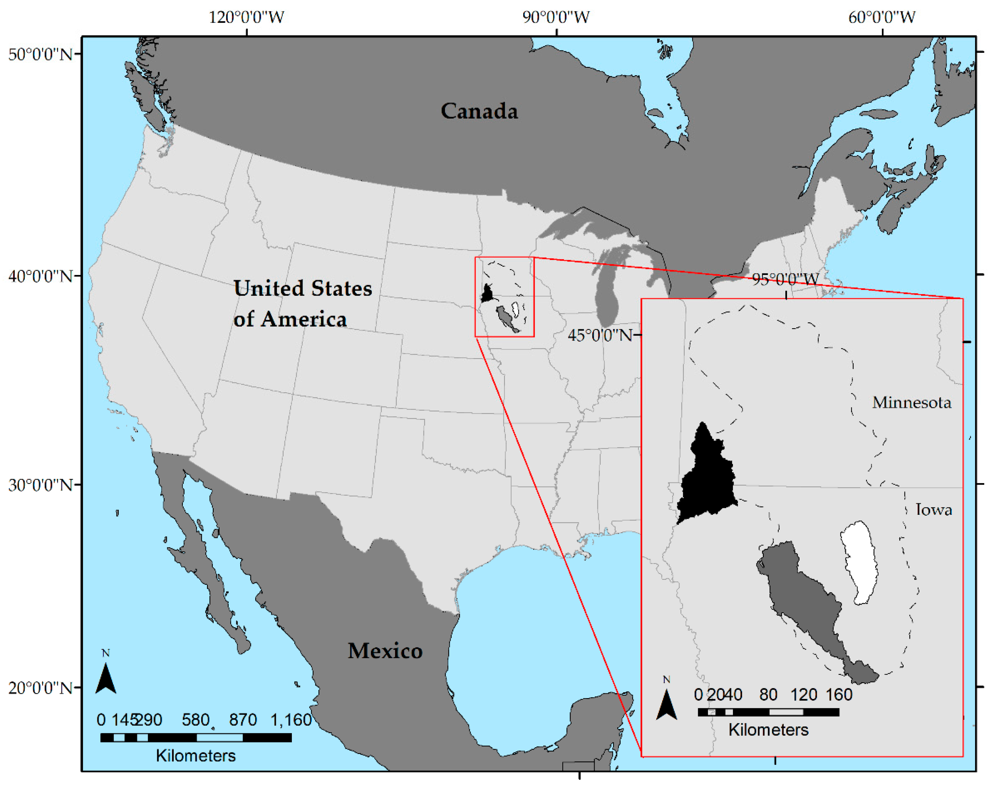
2.1. Study Area

Three 8-digit hydrologic unit code (HUC 8) watersheds were selected as case studies for this process: the North Raccoon River watershed (HUC 07100006), the Boone River watershed (HUC 07100005), and the Rock River watershed (HUC 10170204; Figure 1). Hydrological unit codes (HUC)s are hierarchical numeric identifiers assigned by the U.S. Geological Society (USGS) to watersheds in the United States of America. The number of digits comprising the HUC is representative of the size of the watershed with increasing digits representing smaller sub-watersheds. HUC 8 watersheds represent sub-basins. The multiple HUC 8 scales were selected for this study as they represent the areas at which managers are currently conducting oxbow restorations in Iowa and Minnesota. These watersheds were selected because they are the focus of ongoing oxbow restoration activities for Topeka Shiner conservation. The North Raccoon and Boone River watersheds are in west-central Iowa in the Des Moines Lobe ecoregion that is characterized by low-relief topography as a result of glacial retreat following the last ice age [45]. Both watersheds are heavily altered by intensive row crop agriculture and channelization of streams; many headwater streams in the Midwestern United States have been altered to extend into drainage ditches to support row crop agriculture [10]. The Rock River watershed is bisected by the Iowa/Minnesota state boundary, and it is located within the Loess Prairies ecoregion. Like the North Raccoon and Boone River watersheds, the Rock River watershed has low relief topography and is dominated by row crop agriculture [45].

2.2. Data Acquisition

The original DEMs for each watershed were obtained as bare earth LiDAR-derived DEMs with 2 m horizontal resolution organized by local basins within the HUC 8 sub-basins (HUC 12) watershed geodatabases. These HUC 12 DEMs were merged into HUC 8 DEMs for preprocessing. DEMs all had a vertical positional accuracy of ~18.5 cm, and they were obtained through Iowa State University. DEMs that represented area within the Iowa state boundary were hydrologically enforced prior to acquisition to ensure proper hydrological flow via an automated process developed at Iowa State University [28]. DEMs that represented area within Minnesota state boundaries had not previously undergone a hydroconditioning process. To enforce proper hydrological flow in all watersheds, we implemented a hydroconditioning process as described below in Section 2.3. Field boundaries and use characteristics for all watersheds were downloaded from the agricultural conservation and planning framework (ACPF) Watershed Database Land Use Viewing and Data Downloading website [46]. The field boundaries dataset was digitized for many of the Midwestern states through examination of aerial imagery by ACPF users. In the field boundaries dataset, a general land use attribute (IsAG) was assigned to each field boundary shapefile. Broadly, a value of 1 designates fields used for crop agriculture, a value of 2 designates a field used for pasture, and a value of 0 designates a non-agricultural field [47,48].

2.3. Preprocessing

The methodology described in this paper requires a DEM, corresponding stream network, field boundary dataset, and a relative elevation raster dataset. If these data are unavailable, some preprocessing is required and is described in detail in this section. All processing for this study was completed using ArcGIS 10.4.1 by ESRI ©. Minnesota DEMs were hydroconditioned using the ACPF toolbox by manually correcting the DEM to force stream networks to flow underneath structures such as bridges or culverts instead of backing up behind them [49]. Though Iowa DEMs had undergone an automated hydroconditioning process, these DEMs were quality controlled using the ACPF toolbox to ensure proper flow. Stream networks were delineated again using the ACPF toolbox and using a 40.47 ha drainage threshold for all watersheds [47]. The 40.47 ha drainage threshold was selected as it generated a stream network that accurately captured the total extent of perennial streams and drainage ditches in all three watersheds as verified by aerial imagery examination. The ACPF toolbox preprocessing methodology begins by creating a filled DEM using the default Fill tool in ESRI ArcGIS without predetermined thresholds. The Fill tool eliminates depressions across the landscape by filling sinks. Next, the ACPF toolbox generates a D8 Flow Direction and D8 Flow Accumulation raster dataset that allows for the generation of a stream network. D8 Flow direction and D8 flow accumulation considers elevation difference and slope to assign hydrological movement to one of 8 directions: East, Northeast, North, Northwest, West, Southwest, South, and Southeast [50]. The ACPF hydroconditioning process involves the iterative creation of stream networks, identification of incorrect flow, and manual editing of the DEM to force proper flow. Once a hydrologically accurate flow network is created, stream segments are manually coded using the editor toolbar as either false flowpaths/intermittent streams (0), perennial streams (1), or drainage ditches (4). Areas in which the flow path extended past the terminus of a perennial stream or drainage ditch were split and the excess line was coded as a 0. Final designations of perennial streams and drainage ditches were created with the ACPF tool “Stream Reach & Catchments” to generate a final stream network for each watershed. Finally, a relative elevation dataset, hereafter referred to as “height above channel,” was calculated from the DEMs so each cell resulted in height (cm) above the nearest stream cell to which it would flow.

2.4. Riparian Depression Identification

Search radius for depressions was limited to a 500 m buffer around stream segments coded as perennial to comply with USFWS restoration practice. A distance of 500 m was chosen after visual examination of the study area determined it was an appropriate distance to consistently incorporate all oxbows and former meanders within the floodplains of all watersheds within both ecoregions. The original hydroconditioned DEM (oDEM), the Filled DEM (fDEM), and the height above channel (HAC) dataset were extracted to the 500 m buffer. Depressions were identified by subtracting the oDEM from the fDEM and then converting the contiguous areas not equal to 0 to shapefiles representing depressions across the landscape. Depressions with areas ≤ 100 m² were eliminated from the analysis because they were considered too small to represent target features. Depressions intersecting the stream network were also eliminated from consideration because oxbow habitats are typically isolated from the main stream channel during base flows. The USFWS does not perform restorations in active row crop agricultural fields as these areas could be impacted by additional nutrient run-off [40]. However, depressions within pasture fields were retained because restorations in pastures do not interfere with cattle grazing and Topeka Shiners appear to co-exist with cattle in these environments [37,40]. Field boundary shapefiles were converted to raster datasets and reclassified to only include row crop agricultural fields. Using the “Tabulate Area” tool in ArcGIS area covered by a row crop agricultural field was calculated for each depression. If less than 100 m² of the feature was outside an agricultural field, the depression was excluded as a potential restoration site.

2.5. Model Creation and Evaluation

Each of the depression features identified within 500 m of the perennial streams in the three watersheds of study were assigned several morphometric and topographic characteristics that were all considered in the development of classification tree models to discriminate between target and non-target features. Topographic characteristics included: mean depth, maximum depth, mean slope, mean surface roughness, and mean relative height above channel. These variables were calculated for each depression using the “Zonal Statistics as Table” tool in ArcGIS. Surface roughness was also included as a topographic characteristic and was determined by using a 5 cell moving focal window to calculate the standard deviation of the depression’s slope [51]. Circularity, solidity, convexity, concavity, rectangularity, area, and perimeter were calculated to describe the morphometric characteristics of each depression (

Table 1. Morphometric features calculated for each depression to characterize its shape. Circularity (CIR) compares the shape to a circle; values approaching 1 indicate a more circular depression. Solidity describes the extent to which a shape is concave or convex. Rectangularity compares how closely the depression resembles a rectangle. Concavity is the extent that a shape is concave. Convexity is the extent a shape is convex.

Morphometric Characteristic	Formula	Shapes Representing the Extremes of Each Metric
Circularity (CIR)	$=\frac{P_d}{2\sqrt{\pi A_d}}$
Solidity (SLD)	$=\frac{A_d}{A_{ch}}$
Rectangularity (REC)	$=\frac{A_d}{\left(2L\ast 2W\right)}$
Convexity (CVX)	$=\frac{P_{ch}}{P_d}$
Concavity (CON)	$=\sqrt{{\left(1-SLD\right)}^2+{\left(1-CVX\right)}^2}$

Abbreviations: $A_d$: Area of the depression; $P_d$: Perimeter of the depression; $A_{ch}$: Area of the minimum bounding convex hull; $P_{ch}$: Perimeter of the minimum bounding convex hull; L: Length of the minimum bounding rectangle by width; W: Width of the minimum bounding rectangle by width.

).

To build and evaluate a classification tree model that would assess the ability of the variables to differentiate target riparian features (oxbows, oxbow scars, and relic stream meanders) we created a pool of target and non-target features by manually coding each depression as either a 0 (non-target features) or a 1 (target features; Figure 2). Depressions were coded by two researchers independently using both historical and recent USDA orthoimagery from the 1930s, 1950s, 1960s, 1970s, 1980s, 1990s, and 2015 [52]. Disagreements in feature designation were re-examined, and a final decision was made. Criteria for coding a depression as a target feature included:

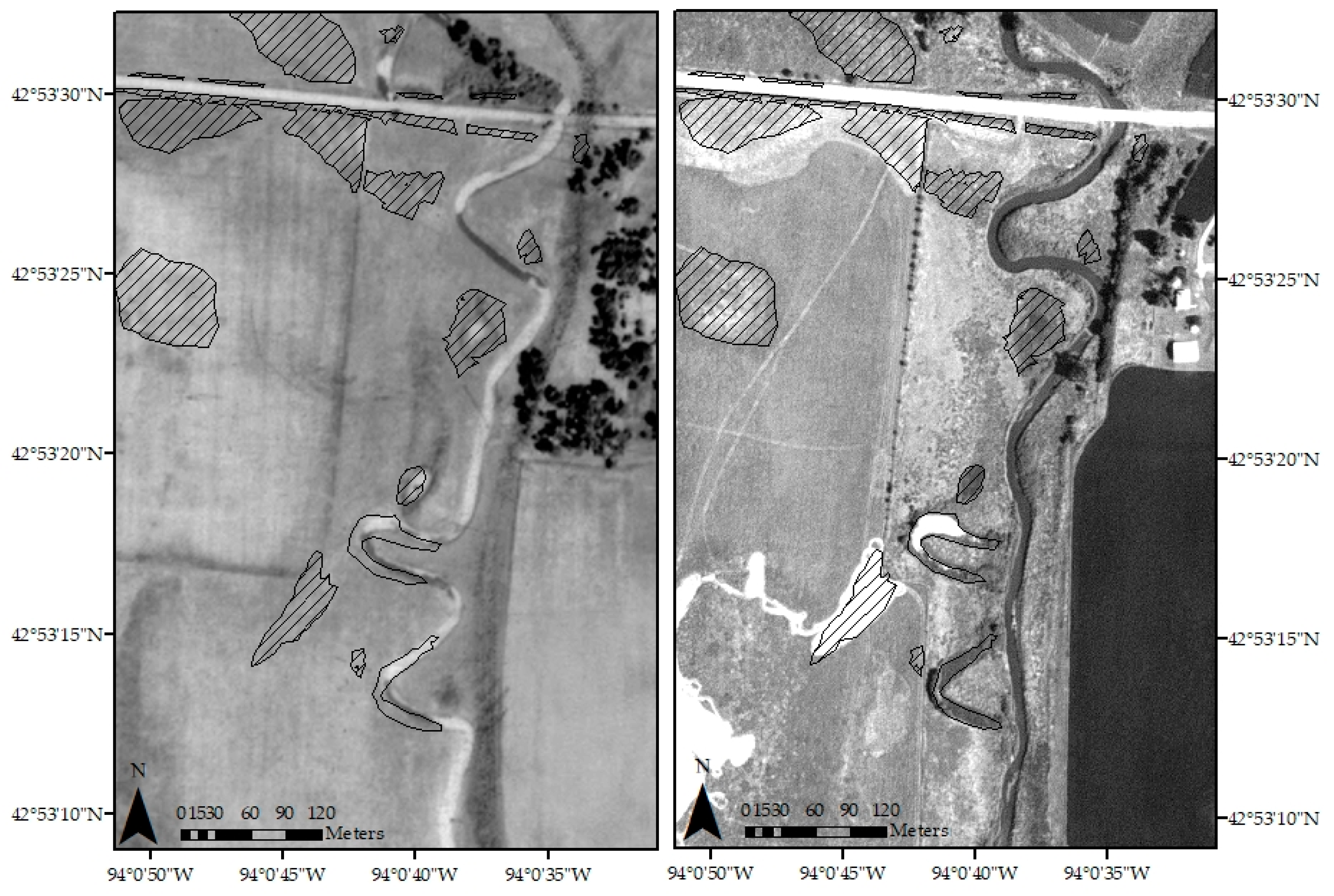
• Intersection with either a stream channel, oxbow, or oxbow scar within one aerial image
• Maintenance of the original shape of the historical channel, oxbow, or oxbow scar

Though time intensive, this manual coding was necessary to capture a pool of data large enough to develop robust models as target features were rare in all watersheds comprising only ~2–4% of all depressions initially identified (

Table 2. The initial number of depressions identified within 500 m buffer of perennial streams by watersheds. The depressions that had <100 m² area outside an agricultural field and depressions that intersect the stream were excluded from analyses.

Watershed/Watershed Combination	Total Depressions	Non-target Features	Target Features	% Target Features
Boone River Watershed	9278	9047	231	2.49
North Raccoon River Watershed	33,485	32,719	766	2.29
Des Moines Lobe Watersheds	42,763	41,766	997	2.33
Rock River Watershed	22,411	21,491	920	4.11
All-watersheds combined	65,174	63,257	1917	2.94

).

Data from watersheds were analyzed by individual watersheds, by ecoregion, and by watersheds combined to assess both the overall accuracy of separating oxbow features from other riparian depressions as well as to analyze how oxbow identification varied among study area. Thus, a training dataset and testing dataset were generated by randomly splitting the data without replacement so 80% was apportioned to a training dataset to train a classification tree model. The remaining 20% of the data was used to test the performance of the generated model.

Imbalanced datasets, such as ours, with target features representing only a small portion of all features identified, are problematic as most modeling algorithms are designed to minimize total error and are more accurate with even splits between classes [53]. To account for the unbalanced dataset the training data were further split so that all target features were preserved and set as 50% of the final training data while the majority non-target features were randomly under-sampled without replacement to comprise the remaining 50% of the final training dataset. This final training dataset underwent a 10-fold cross-validation process before final model creation. The performance of each model was evaluated by its specificity (true negative rate), sensitivity (true positive rate), precision (rate at which target feature designations were correct), correct classification rate, and area under the curve (AUC) of the receiver operator curve [54,55]. To overcome the effect of noise, target features were ranked on how likely they were to be an oxbow by normalizing each node’s conditional probability. Conditional probabilities were calculated for each depression based on percentage of correctly classified depressions at the terminus of all target feature nodes. Conditional probabilities were then reclassified to range between 0–7. Depressions with a 0 value were classified by the model as a target depression, however, they were more likely to be noise than depressions with a value of 7 which had the greatest likelihood of being a target feature.

3. Results

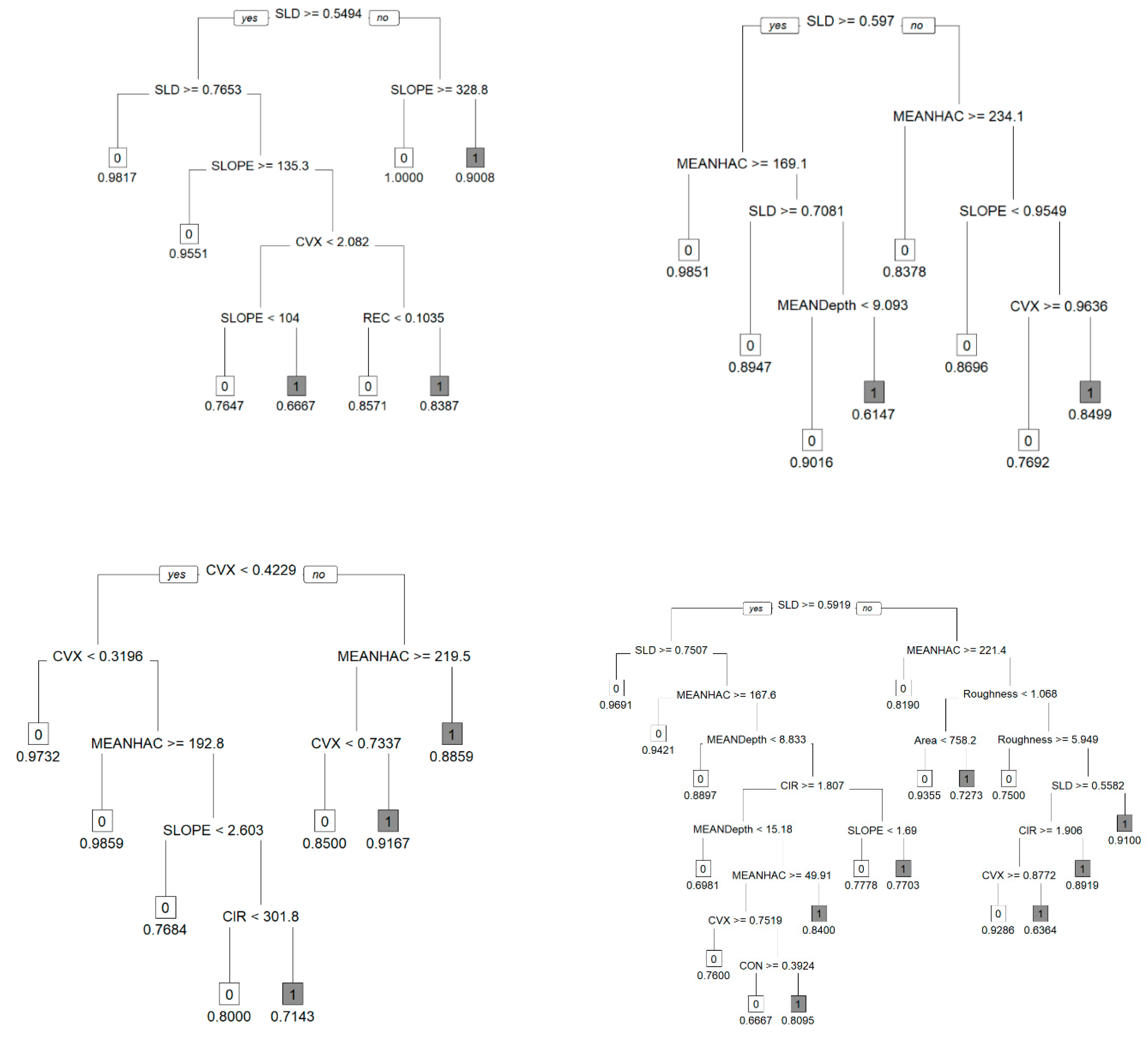
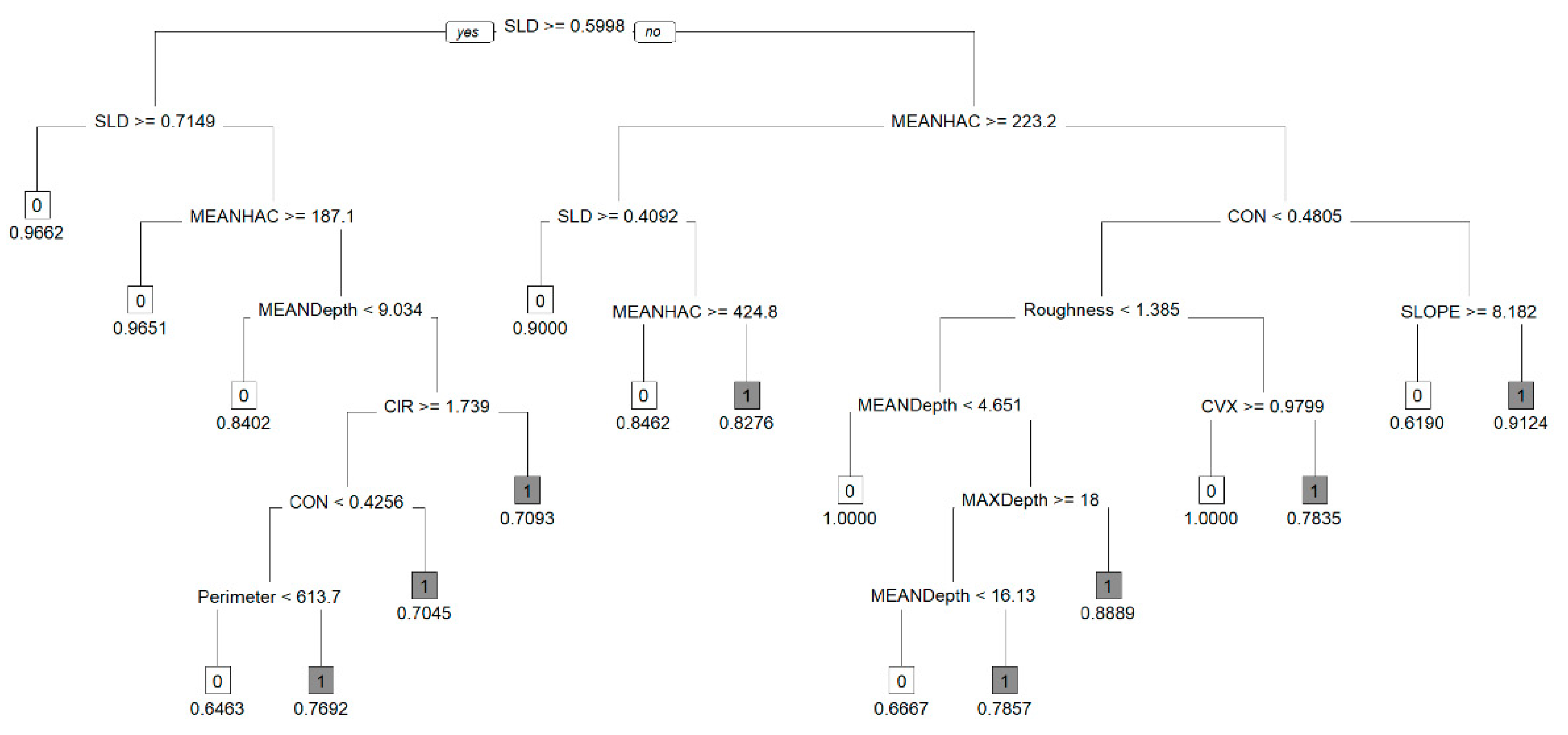
3.1. Model Accuracies

Classification trees were created for all watersheds individually, watersheds by ecoregion, and all watersheds combined (Figure 3). The morphometric characteristic solidity represented the first split in all models except the Rock River watershed model. Generally, features with low solidity values were classified as target features. Mean relative HAC was one of the second tier splits in all models except the Boone River watershed and suggested that features with a lower mean relative HAC were classified as target features. Mean depth of each feature was present in the North Raccoon River, Des Moines Lobe ecoregion, and the all-combined watershed models. Perimeter was only used to classify features in the all-watershed combined models. Depression feature area was included in the Des Moines Lobe ecoregion watershed models, but absent in the others. Mean roughness of the depression’s surface was included in the Des Moines Lobe ecoregion and all-watershed combined model. Circularity was included in the Rock River, Des Moines Lobe ecoregion, and the all-watershed combined models. Convexity and mean slope were included all models.

Confusion matrices were created for all models to calculate specificity, sensitivity, precision, and correct classification rate for all model combinations (

Table 3. The specificity (true negative rate), sensitivity (true positive rate), precision (rate at which features classified as a target feature were true target features), correct classification rate, and area under the receiver operator curve (AUC) of each model.

Watershed	Specificity	Sensitivity	Precision	Correct Classification Rate	AUC
Boone	0.89	0.75	0.16	0.88	0.82
North Raccoon	0.91	0.83	0.19	0.91	0.87
Des Moines Lobe	0.92	0.80	0.20	0.91	0.86
Rock River	0.94	0.89	0.39	0.94	0.91
All-watershed	0.93	0.82	0.26	0.92	0.87

). All models had specificity values greater than 0.89 indicating that the models were successful in correctly classifying non-target features. Sensitivity rates ranged from 0.75 in the Boone River watershed to 0.89 in the Rock River watershed indicating that though the models were less successful at correctly classifying true target features than correctly classifying non-target features, the models still performed well. Precision, or the expression of how often a feature that was classified by the model as a target feature was a true target feature, varied widely across watersheds with the lowest precision in the Boone River watershed and the greatest precision in the Rock River watershed. Correct classification rates (CCR) of all models ranged between 0.88–0.94.

AUC scores range from 0 to 1 with higher scores representing more accurate models and models with an AUC score of 0.5 indicate the model performs no better than random choice. Overall, the Rock River watershed had the highest AUC score of 0.91 followed by the North Raccoon River, all-watershed combined models, and Des Moines Lobe ecoregion with AUC scores of 0.87, 0.87, and 0.86 respectively (Table 3). The Boone River watershed model had the lowest AUC value of 0.82. All models performed well, receiving AUC scores considered good or excellent.

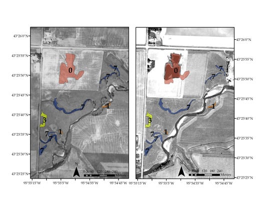
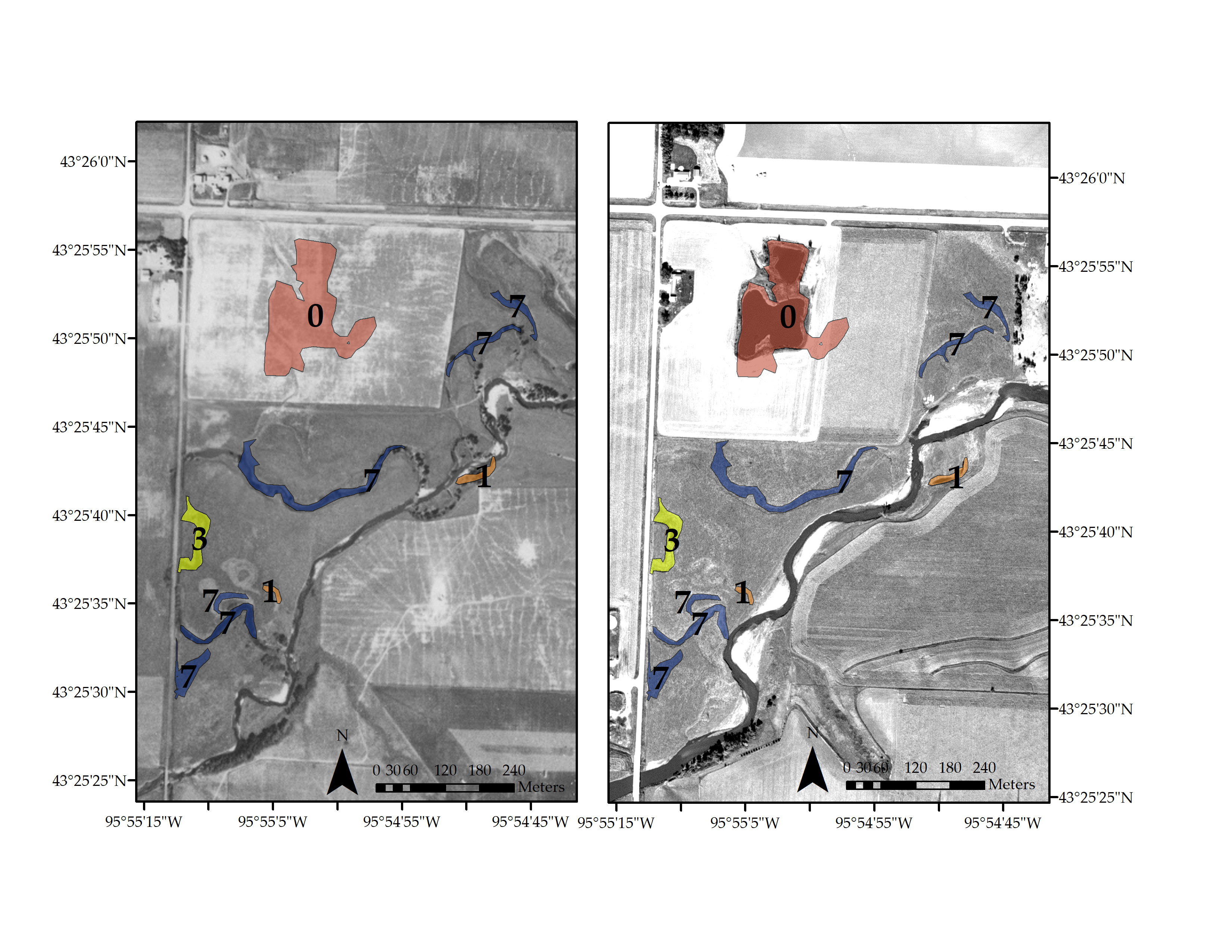
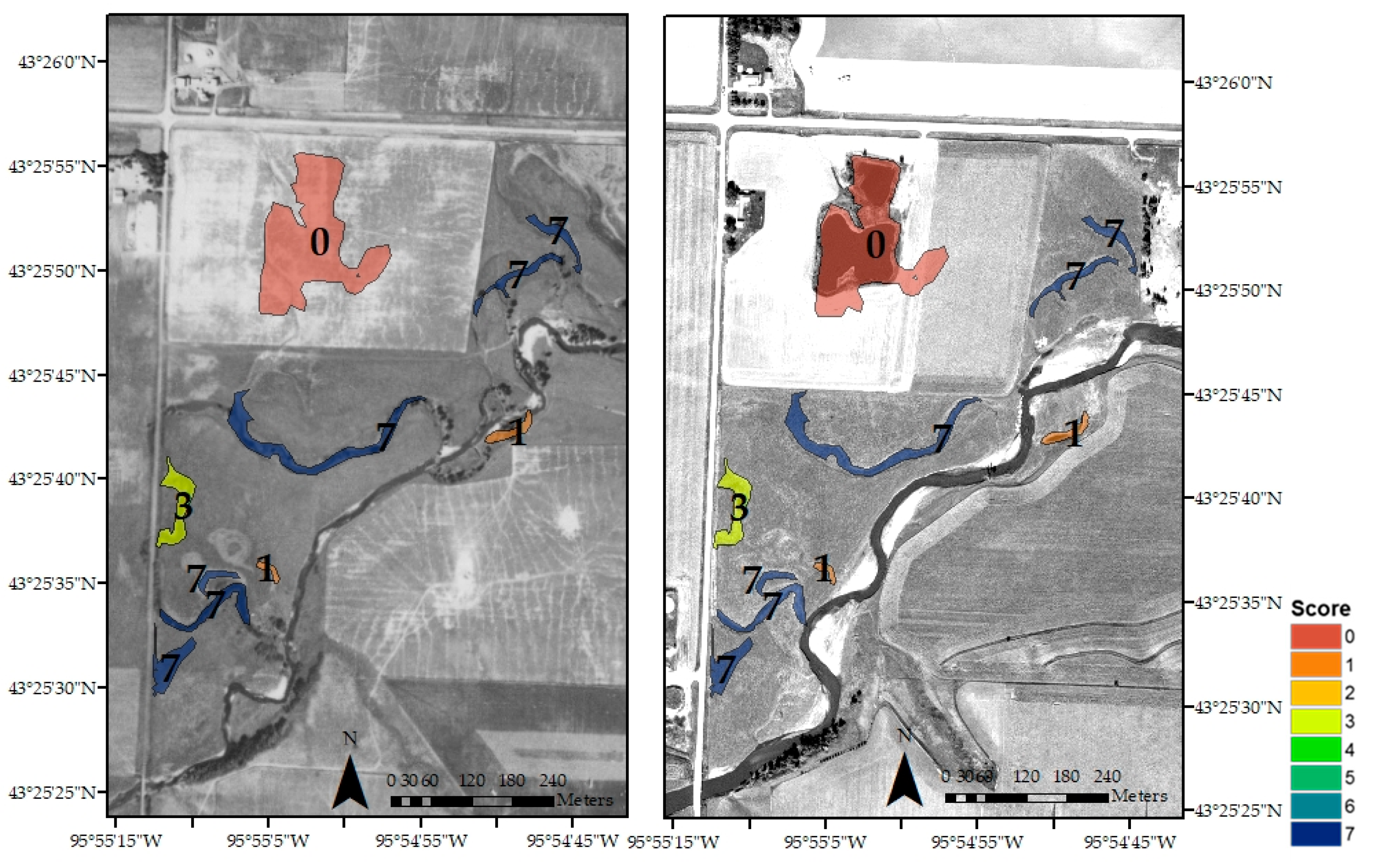
3.2. Model Accuracy at Identifying Chosen Restoration Sites

Because the all-watershed combined model performed well in most evaluation characteristics, its results were chosen to compare to the locations of restored sites for Topeka Shiner conservation. Locations of 127 restoration sites constructed between 2002 and 2017 were compared to the model. Restored sites that were within a 50 m radius of an identified depression were considered part of the same feature as the modeled sites. Sixty-four (50%) restored oxbows habitats in all watersheds were identified as candidate sites by using the all-watershed combined model. The model was most successful at selecting sites that had been chosen for restoration in the Boone River watershed by identifying ten out of seventeen sites (59%). The overall model identified nineteen out of forty-four (43%) restored sites in the Rock River watershed and thirty-five out of sixty-six restored sites (53%) in the North Raccoon River watershed. Non-selection of restored sites by the model was primarily related to either the omission of a detected depression, or the direct connection of a depression to the stream channel which caused it to be excluded from the initial depression pool.

3.3. Ranking Sites

The all combined watershed model classified eight terminal nodes on the classification trees as target features (Figure 4). All features associated with the target feature nodes were selected as potential oxbow restoration sites. Of the 65,174 originally identified riparian depressions, the all-watershed model identified 7650 (11.74%) of those depressions as target features across all three watersheds of study. Though the possible sites were reduced drastically, we further chose to rank identified features to identify top candidate sites by how likely they were to be our classified target features. Conditional probabilities of each node were calculated by the probability of the node’s fitted class. Target feature nodes’ conditional probability ranged from 0.7093 to 0.9124. Because eight nodes were identified, features were ranked from 0 to 7 with the lowest rank corresponding to the lowest conditional probability (Figure 4). The highest rank of features (Rank 7) accounted for 3521 (46.03%) of the identified target features and thus was able to further reduce the top candidate sites for managers to consider for restoration. Sites with lower ranks may be low-lying landscape features that have irregular shapes such as constructed ponds or wetlands while higher ranked features were more likely to be historical stream meanders (Figure 4). Though this ranking methodology did help further identify the best target sites, it did highlight an area of noise of irregular shapes created by proximity to roads, leading to curved shapes that may be inaccurately identified as a relic stream channel or oxbow (Figure 4).

4. Discussion

The growing availability of high-resolution LiDAR-derived digital elevation models has allowed for the development of methodologies to classify target features across wide swathes of the earth’s surface. Oxbows and other off-channel habitats are important floodplain features that provide habitat for fish species at a variety of life stages [6,56,57]. Following European settlement, the Midwestern United States lost much of its historical hydrological complexity to the creation of drainage ditches and tile installation to support expansive row crop agriculture [58,59,60]. Restoration of off-channel habitats for the conservation of the endangered Topeka Shiner began in 2002 and continues to be a conservation strategy of USFWS to increase suitable habitat. This methodology follows the similar efforts of other studies to develop parameters that will identify potential target landscape features and help guide restoration site selection by providing an objective, repeatable practice [28,61,62,63]. Our study demonstrated our ability to extract the unique features of relic stream channels, oxbow scars, and oxbows from other riparian depressions across the landscape from LiDAR-derived digital elevation models.

Overall model accuracy in correctly labeling features as either target or non-target was above 88% in all models. Previous literature demonstrates the utility of shape characteristics such as ellipticity, circularity, form factor, area, volume, and solidity [64,65,66,67,68]. Because former stream meanders and oxbows have unique shape characteristics, we aimed to identify parameters that would characterize this pattern. Both solidity and relative height above channel variables were important in identifying oxbows and relic channels. Solidity is an intuitive defining characteristic, as oxbows have a classic horseshoe shape and relic streams are often naturally meandering with alternating concave and convex segments. Mean relative height above channel was also expected to be important in discriminating target features from non–target features because former meanders were once part of the stream network and their relative elevation to the channel is similar until sediment deposition eventually fills them with silt [69]. Older features, such as older oxbow scars, will have a greater relative elevation than a newly formed oxbow that was recently isolated from the stream. Occasionally, we observed that classic oxbow shapes were formed when drainage ditches artificially bisected a natural, meandering stream. Improved classification rates may be achieved by expanding response variables from a binary target/non-target classification to additional classes to discriminate relic streams, oxbows, and oxbow scars separately. The model did not separate target features into their individual classifications because the highly modified nature of the landscape proved difficult to visually separate these features for validation.

Though our models correctly classified target features, we observed that when applied to large areas the process produced numerous features that were false positive detections. This observation in part was due to the enormous quantity of depressions identified in the riparian zone as the pool of initial candidate sites. Though only a small percentage of misclassification of non-target features (~7%) were observed in the all-watershed combined model, this small percentage of 63,257 non-target features yielded many physical features that were falsely identified on the landscape as potential restoration sites. To compensate for this we believe the addition of the ranking system aids in the practical application of this process as it allows managers to sift through some of the misclassified features. Additionally, though we did not specifically address human classification accuracy for oxbows, so the prevalence of misclassification in the model could also be due to human error while classifying target versus non-target features. This human error could stem from the difficulty of identifying historical stream meanders in highly modified environments as well as the fact that our aerial imagery data was only available after the 1930s despite modification of the Midwestern landscape beginning many decades earlier.

Through visual comparison of the features identified with this model to those sites previously selected as restoration locations, we observed that several restoration sites were missed by our model because they intersected with the stream and were thus eliminated from consideration. A recent methodology that shows promise to mitigate this issue is the delineation of nested depressions, or the extraction of depressions that are within larger depressed areas such as highly connected stream channel [70]. Additionally, the timing and collection of aerial LiDAR could impact the conditions sensed on the earth’s surface, so while the availability of LiDAR data has facilitated much interest in conservation planning, its use should be accompanied by knowledge that conditions can change post-sampling to alter the reality on the surface. The use of this methodology could be integrated into our process for future updates of the tool, and more research is needed to assess its contribution to increasing the accuracy of the model. Though the Normalized Difference Water Index (NDWI) [71] has been used to identify wetland features [28], we elected to limit the scope of this analysis to LiDAR-derived digital elevation models as we aimed to deliver a methodology that are user friendly to managers with limited data processing capacity and/or knowledge of GIS workflows.

Our study demonstrates the utility and feasibility of accurately extracting former stream meander and oxbow lake features from the riparian landscape. Although we observed some misclassification, many of those features were low-lying sinuous areas that included areas of stream swale or other natural riparian depressions. Though not relic meanders or oxbow scars, the misclassified features may present additional opportunities for restoration. This process identifies potential restoration sites and provides information to managers to select appropriate restoration locations, but final site selection should be accompanied by local knowledge, proximity to known Topeka Shiner populations, potential risks to infrastructure such as flooding and erosion, and landowner permission. There is a natural risk to fish that inhabit ephemeral off-channel habitats as extended periods of dry weather can lead to complete desiccation and total fish mortality [11]. Therefore, features with lower elevations relative to the stream channel may be priority sites for restoration as they are more likely to be closely connected to the groundwater via the hyporheic zone. Groundwater percolation into the restored off-channel habitat may be critical for fish survival during extended periods of little or no precipitation. The features identified with our process maintain their relative height above channel data, and this data may be useful for further site selection depending on restoration planners’ goals.

This method provides the initial steps to identify these unique riparian features. This methodology demonstrates that the parameters provided allow for accurate implementation across multiple ecoregions within the Midwestern United States. While our parameters captured the unique and defining sinusoidal pattern of former stream meanders and oxbow lakes, further research is needed to confirm that these parameters can be transferred to other regions. Though this analysis for riparian feature classification was intended to support aquatic species conservation, it may have applications for other conservation efforts. Oxbows restorations have been constructed outside of the Topeka Shiner range in Iowa to help support nutrient reduction efforts. Oxbows significantly reduce nitrate concentrations inputs to the stream from crop fields [72]. This process for identifying candidate sites for oxbow restoration has the potential to not only promote conservation for species such as the Topeka Shiner, but may also support efforts to identify suitable locations to construct oxbow lakes intended to improve regional water quality.

5. Conclusions

A methodology using high-resolution LiDAR-derived digital elevation models was created to identify former stream meanders, oxbows, and oxbow scars. Riparian depression’s solidity, concavity, and mean height above channel were found to be particularity important characteristics in identifying these riparian features, and models performed with AUC scores ≥ 0.82. This methodology was intended to replace time-intensive examination of multi-year aerial imagery and digitization of these features on the landscape. To facilitate widespread use and expand the utility of increasingly available high-resolution LiDAR-derived digital elevation models this methodology was converted into an ArcGIS toolbox. Pre-processing is minimal for this methodology to be implemented, and the preprocessing steps outside of the provided toolbox implementation are described in detail so as to guide future users. Although success in modeling these riparian features by capturing the unique sinusoidal shape and relative elevation to the stream channel was demonstrated across different ecoregions of the Midwestern United States of America, further testing of this process in other regions is an opportunity for further research. This process was developed to support endangered species conservation planning, specifically for Topeka Shiner conservation in Midwestern floodplains, but there are many other species that benefit from floodplain restoration and it may have the potential for application for other species in other regions. Supporting files to this manuscript include a user’s guide and the oxbow identification ArcGIS add-in toolbox are available online in the Supplementary Materials.

References

1. Cramer, M.L. Stream Habitat Restoration Guidelines; Washington Department of Fish and Wildlife: Olympia, WA, USA; Washing Department of Natural Resources: Olympia, WA, USA; Washington Department of Transportation: Olympia, WA, USA; Washington Department of Ecology: Olympia, WA, USA; Washington State Recreation and Conservation Office: Olympia, WA, USA; Puget Sound Partnership: Olympia, WA, USA; U.S. Fish and Wildlife Service: Olympia, WA, USA, 2012.
2. Gallardo, B.; Cabezas, Á.; Gonzalez, E.; Comín, F.A. Effectiveness of a newly created oxbow lake to mitigate habitat loss and increase biodiversity in a regulated floodplain. Restor. Ecol. 2012, 20, 387–394. [Google Scholar] [CrossRef]
3. Landress, C.M. Fish assemblage associations with floodplain connectivity following restoration to benefit an endangered catostomid. Trans. Am. Fish. Soc. 2016, 145, 83–93. [Google Scholar] [CrossRef]
4. Richards, C.; Cernera, P.J.; Ramey, M.P.; Reiser, D.W. Development of off-channel habitats for use by juvenile chinook salmon. N. Am. J. Fish Manag. 1992, 12, 721–727. [Google Scholar] [CrossRef]
5. Scheerer, P.D. Implications of floodplain isolation and connectivity on the conservation of an endangered minnow, Oregon Chub, in the Willamette River, Oregon. Trans. Am. Fish. Soc. 2002, 131, 1070–1080. [Google Scholar] [CrossRef]
6. Junk, W.J.; Bayley, P.B.; Sparks, R.E. The flood pulse concept in river-floodplain systems. Proc. Int. Large River Symp. Can. Spec. Publ. Fish. Aquat. Sci. 1989, 106, 11–127. [Google Scholar]
7. Zeug, S.C.; Winemiller, K.O. Relationships between hydrology, spatial heterogeneity, and fish recruitment dynamics in a temperate floodplain river. River Res. Applic. 2008, 24, 90–102. [Google Scholar] [CrossRef]
8. Zimmer, D.W.; Bachmann, R.W. Effects of Stream Channelization and Bank Stabilization on Warmwater Sport Fish in Iowa: Subproject No. 4. The Effects of Long-Reach Channelization on Habitat and Invertebrate Drift in Some Iowa Streams; U.S. Fish and Wildlife Service: Washington, DC, USA, 1976.
9. Lau, J.K.; Lauer, T.E.; Weinman, M.L. Impacts of channelization on stream habitats and associated fish assemblages in East Central Indiana. Am. Midl. Nat. 2006, 156, 319–330. [Google Scholar] [CrossRef]
10. Urban, M.A.; Rhoads, B.L. Catastrophic human-induced change in stream-channel planform and geometry in an agricultural watershed, Illinois, USA. Ann. Am. Assoc. Geogr. 2003, 93, 783–796. [Google Scholar] [CrossRef]
11. Constantine, J.A.; Dunne, T. Meander cutoff and the controls on the production of oxbow lakes. Geology 2008, 36, 23–26. [Google Scholar] [CrossRef]
12. Ishii, Y.; Hori, K. Formation and infilling of oxbow lakes in the Ishikari lowland, northern Japan. Quat. Int. 2016, 397, 136–146. [Google Scholar] [CrossRef]
13. Gay, G.R.; Gay, H.H.; Gay, H.H.; Martinson, H.A.; Meade, R.H. Evolution of cutoffs across meander necks in Powder River, Montana, USA. Earth Surf. Process. Landf. 1998, 23, 651–662. [Google Scholar] [CrossRef]
14. Fischer, J.R.; Bakevich, B.D.; Shea, C.P.; Pierce, C.L.; Quist, M.C. Floods, drying, habitat connectivity and fish occupancy dynamics in restored and unrestored oxbows of West-Central Iowa, USA. Aquat. Conserv. Mar. Freshw. Ecosyst. 2018, 1–11. [Google Scholar] [CrossRef]
15. Lyon, J.; Stuart, I.; Ramsey, D.; O’Mahony, J. The effect of water level on lateral movements of fish between river and off-channel habitats and implications for management. Mar. Freshw. Res. 2010, 61, 271–278. [Google Scholar] [CrossRef] [Green Version]
16. Miranda, L.E. Fish assemblages in oxbow lakes relative to connectivity with the Mississippi River. Trans. Am. Fish. Soc. 2005, 134, 1480–1489. [Google Scholar] [CrossRef]
17. Hudson, P.F.; Heitmuller, F.T.; Leitch, M.B. Hydrologic connectivity of oxbow lakes along the lower Guadalupe River, Texas: The influence of geomorphic and climatic controls on the “flood pulse concept”. J. Hydrol. 2012, 414–415, 174–183. [Google Scholar] [CrossRef]
18. Buckley, S.J.; Howell, J.A.; Enge, H.D.; Kurz, T.H. Terrestrial laser scanning in geology: Data acquisition, processing, and accuracy. J. Geol. Soc. 2008, 165, 625–638. [Google Scholar] [CrossRef]
19. USGS 3D Elevation Program. Available online: https://www.usgs.gov/core-science-systems/ngp/3dep (accessed on 1 December 2018).
20. Iowa LiDAR Mapping Project. Available online: http://www.geotree.uni.edu/lidar/ (accessed on 1 December 2018).
21. Minnesota Department of Natural Resources. MnTOPO. Available online: https://www.dnr.state.mn.us/maps/mntopo/index.html (accessed on 1 December 2018).
22. Li, S.; MacMillian, R.A.; Lobb, D.A.; McConkey, B.G.; Moulin, A.; Fraser, W.R. Lidar DEM error analysis and topographic depression identification in a hummocky landscape in the prairie region of Canada. Geomorphology 2011, 129, 263–275. [Google Scholar] [CrossRef]
23. Millard, K.; Redden, A.M.; Webster, T.; Stewart, H. Use of GIS and high resolution LiDAR in salt marsh restoration site suitability assessment in the upper Bay of Fundy, Canada. Wetl. Ecol. Manag. 2013, 21, 243–262. [Google Scholar] [CrossRef]
24. Wu, Q.; Lane, C.; Liu, H. An effective method for detecting potential woodland vernal pools using high-resolution LiDAR data and aerial imagery. Remote Sens. 2014, 6, 11444–11467. [Google Scholar] [CrossRef]
25. Wu, Q.; Lane, C.R. Delineation and quantification of wetland depressions in the prairie pothole region of North Dakota. Wetlands 2016, 36, 215–227. [Google Scholar] [CrossRef]
26. Terefenko, P.; Wziatek, D.Z.; Dalyot, S.; Boski, T.; Lima-Filho, F.P. A High-Precision LiDAR-Based Methodology for Surveying and Classifying Coastal Notches. J. Geol. Soc. 2018, 7, 295. [Google Scholar] [CrossRef]
27. Whitney, G.G. From Coastal Wilderness to Fruited Plain: A History of Environmental Change in Temperate North America from 1500 to the Present; Cambridge University Press: Cambridge, UK, 1996; ISBN 0 521 57658 X. [Google Scholar]
28. Gelder, B.K. Automation of DEM Cutting for Hydrologic/Hydraulic Modeling; Technical Report; Iowa State University Institution for Transportation: Ames, IA, USA, 2015. [Google Scholar]
29. Tabor, V.M. Final Rule to List the Topeka Shiner as Endangered; Federal Register 63:240; U.S. Department of the Interior, U.S. Fish and Wildlife Service: Manhattan, KS, USA, 1998; pp. 69008–69021. 26p. Available online: https://www.gpo.gov/fdsys/pkg/FR-1998-12-15/pdf/98-33100.pdf (accessed on 13 August 2017).
30. Bakevich, B.D.; Pierce, C.L.; Quist, M.C. Status of the Topeka Shiner in West-Central Iowa. Am. Midl. Nat. 2015, 174, 350–358. [Google Scholar] [CrossRef] [Green Version]
31. Zambory, C.L.; Bybel, A.P.; Pierce, C.L.; Roe, K.J.; Weber, M.J. Habitat Improvement Projects for Stream and Oxbow Fish of Greatest Conservation Need; Annual Progress Report; Iowa State University: Ames, IA, USA, 2017; Available online: https://www.cfwru.iastate.edu/files/project/files/2016_swgc_annualreport_final.pdf (accessed on 20 January 2017).
32. Simpson, N.T.; Pierce, C.L.; Roe, K.J.; Weber, M.J. Boone River Watershed Stream Fish and Habitat Monitoring, IA; Annual Progress Report; Iowa State University: Ames, IA, USA, 2016; Available online: https://www.cfwru.iastate.edu/files/project/files/2016_brw_annualreport_final.pdf (accessed on 20 January 2017).
33. Clark, S.J. Relationship of Topeka Shiner Distribution to Geographical Features of the Des Moines Lobe in Iowa. Master’s Thesis, Iowa State University, Ames, IA, USA, 2000. [Google Scholar]
34. Berg, J.A.; Petersen, T.A.; Anderson, Y.; Baker, R. Hydrogeology of the Rock River Watershed, Minnesota and Associated Off-Channel Habitats of the Topeka Shiner. Final Report Submitted by the Minnesota Department of Natural Resources 2004. Available online: http://files.dnr.state.mn.us/eco/nongame/projects/consgrant_reports/2004/2004_berg_etal.pdf (accessed on 13 November 2017).
35. Bakevich, B.D.; Pierce, C.L.; Quist, M.C. Habitat, fish species, and fish assemblage associations of the Topeka Shiner in West-Central Iowa. N. Am. J. Fish Manag. 2013, 33, 1258–1268. [Google Scholar] [CrossRef]
36. Hatch, J.T. What we know about Minnesota’s first endangered fish species: The Topeka shiner. J. Minn. Acad. Sci. 2001, 65, 39–46. [Google Scholar]
37. Thomson, S. Dugouts and stream fishes, especially the endangered Topeka Shiner; U.S. Department of Agriculture, Natural Resources Conservation Service: Washington, DC, USA, 2010. Available online: https://directives.sc.egov.usda.gov/OpenNonWebContent.aspx?content=29145.wba (accessed on 1 November 2018).
38. Thomson, S.K.; Berry, C.R., Jr.; Niehs, C.A.; Wall, S.S. Constructed impoundments in the floodplain: A source or sink for native prairie fishes, in particular the endangered Topeka shiner (Notropis topeka)? In Proceedings of the 2005 Watershed Management Conference, Williamsburg, VA, USA, 19–22 July 2005. [Google Scholar] [CrossRef]
39. Koehle, J.J.; Adelman, I.R. The effects of temperature, dissolved oxygen, and Asian tapeworm infection on growth and survival of the Topeka shiner. Trans. Am. Fish. Soc. 2007, 136, 1607–1613. [Google Scholar] [CrossRef]
40. Kenny, A. The Topeka Shiner: Shining a Spotlight on an Iowa Success Story. Endangered Species Program News Bulletin. 2013. Available online: https://www.fws.gov/endangered/news/episodes/bu-01-2013/story3/. (accessed on 13 November 2017).
41. Kenny, A.; United States Fish and Wildlife Service, Rock Island, IL, USA. Personal communication, 2017.
42. Ralston, S.; United States Fish and Wildlife Service, Windom, MN, USA. Personal communication, 2016.
43. Heit, M.; Parker, H.; Shortreid, A. GIS Applications in Natural Resources; GIS World Books: Fort Collins, CO, USA, 1991; ISBN 1882610172. [Google Scholar]
44. Wilson, J.P.; Gallant, J.C. Terrain Analysis: Principles and Applications; Wiley: New York, NY, USA, 2000; ISBN 0471321885. [Google Scholar]
45. Griffith, G.E.; Omernik, J.M.; Wilton, T.F.; Pierson, S.M. Ecoregions and subregions of Iowa: A framework for water quality assessment and management. J. Iowa Acad. Sci. 1994, 101, 5–13. [Google Scholar]
46. Iowa State University Geographic Information Systems Facility ACPF DEM Download. Available online: https://www.gis.iastate.edu/gisf/projects/acpf. (accessed on 4 August 2016).
47. ACPF Watershed Database Land Use Viewing and Data Downloading. Available online: https://www.nrrig.mwa.ars.usda.gov/st40_huc/dwnldACPF.html (accessed on 25 July 2017).
48. Tomer, M.D.; James, D.E.; Sandoval-Green, M.J. Agricultural Conservation Planning Framework: 3. Land Use and Field Boundary Database Development and Structure. J. Environ. Qual. 2017, 46, 676–686. [Google Scholar] [CrossRef] [PubMed]
49. Watershed Planning Tool: Agricultural Conservation Planning Framework (ACPF). Available online: http://northcentralwater.org/acpf/ (accessed on 4 August 2016).
50. Tarboton, D.G. Terrain Analysis Using Digital Elevation Models (Taudem). Utah Water Research Laboratory, Utah State University. 2016. Available online: http://hydrology. usu.edu/taudem/taudem5/support.html (accessed on 1 December 2018).
51. Grohmann, C.H.; Smith, M.J.; Riccomini, C. Multiscale Analysis of Topographic Surface Roughness in the Midland Valley, Scotland. IEEE Trans. Geosci. Remote Sens. 2011, 49, 1200–1213. [Google Scholar] [CrossRef] [Green Version]
52. Iowa Geographic Map Server. Available online: https://ortho.gis.iastate.edu/ (accessed on 13 November 2017).
53. Japkowicz, N.; Stephen, S. The class imbalance problem: A systematic study. Intelligent Data Analysis. Intell. Data Anal. 2002, 6, 429–449. [Google Scholar] [CrossRef]
54. Duda, R.O.; Hart, P.E.; Stork, D.G. Pattern Classification, 2nd ed.; Wiley: New York, NY, USA, 2001; ISBN 0471056693. [Google Scholar]
55. Bradley, A.P. The use of the area under the ROC curve in the evaluation of machine learning algorithms. Pattern Recognit. 1997, 30, 1145–1159. [Google Scholar] [CrossRef] [Green Version]
56. Górski, K.; De Leeuw, J.J.; Winter, H.V.; Vekhov, D.A.; Minin, A.E.; Buijse, A.D.; Nagelkerke, A.J. Fish recruitment in a large, temperate floodplain: The importance of annual flooding, temperature and habitat complexity. Freshw. Biol. 2011, 56, 2210–2225. [Google Scholar] [CrossRef]
57. Johnson, G.E.; Ploskey, G.R.; Sather, N.K.; Teel, D.K. Residence times of juvenile salmon and steelhead in off-channel tidal freshwater habitats, Columbia River, USA. Can. J. Fish. Aquat. Sci. 2015, 72, 684–696. [Google Scholar] [CrossRef]
58. Bishop, R.A. Iowa’s wetlands. Proc. Iowa Acad. Sci. 1981, 88, 11–16. [Google Scholar]
59. Smith, D.D. Iowa prairie—An endangered ecosystem. Proc. Iowa Acad. Sci. 1981, 88, 7–10. [Google Scholar]
60. Zucker, L.A.; Brown, L.C. Agricultural Drainage: Water Quality Impacts and Subsurface Drainage Studies in the Midwest; Ohio State University Extension: Columbus, OH, USA, 1998. [Google Scholar]
61. Chirol, C.; Haigh, I.D.; Pontee, N.; Thompson, C.E.; Gallop, S.L. Parametrizing tidal creek morphology in mature saltmarshes using semi-automated extraction from lidar. Remote Sens. Environ. 2018, 209, 291–311. [Google Scholar] [CrossRef]
62. Waz, A.; Creed, I.F. Automated Techniques to Identify Lost and Restorable Wetlands in the Prairie Pothole Regions. Wetlands 2017, 37, 1079–1091. [Google Scholar] [CrossRef]
63. McDeid, S.M.; Green, D.L.; Crumpton, W.G. Morphology of Drained Upland Depressions on the Des Moines Lobe of Iowa. Wetlands 2018, 1–14. [Google Scholar] [CrossRef]
64. Conger, C.L.; Fletcher, C.H.; Hochberg, E.H.; Frazer, N.; Rooney, J.J.B. Remote sensing of sand distribution patterns across an insular shelf: Oahu, Hawaii. Mar. Geol. 2009, 267, 175–190. [Google Scholar] [CrossRef]
65. Doctor, D.H.; Young, J.A. An Evaluation of Automated GIS Tools for Delineating Karst Sinkholes and Closed Depressions from 1-Meter LiDAR-Derived Digital Elevation Data. In Proceedings of the NCKRI Symposium 13th Sinkhole Conference, Carlsbad, NM, USA, 6–10 May 2013; pp. 449–458. [Google Scholar]
66. Zhu, J.; Pierskalla, W.P., Jr. Applying a weighted random forests method to extract karst sinkholes from LiDAR data. J. Hydrol. 2016, 533, 343–352. [Google Scholar] [CrossRef]
67. Chen, H.; Oguchi, T.; Wu, P. Morphometric analysis of sinkholes using a semi-automatic approach in Zhijin County, China. Arab. J. Geosci. 2018, 11, 1–14. [Google Scholar] [CrossRef]
68. Stout, J.C.; Belmont, P. TerEx Toolbox for semi-automated selection of fluvial terrace and floodplain features from lidar. Hydrol. Earth Syst. Sci. 2013, 39, 569–580. [Google Scholar] [CrossRef]
69. Fink, D.F.; Mitsch, W.J. Hydrology and nutrient biogeochemistry in a created river diversion oxbow wetland. Ecol. Eng. 2006, 30, 93–102. [Google Scholar] [CrossRef]
70. Wu, Q.; Lane, C.R.; Wang, L.; Vanderhoof, M.K.; Christensen, J.R.; Liu, H. Efficient delineation of nested depression hierarchy in digital elevation models for hydrological analysis using level-set method. J. Am. Water Resour. Assoc. 2018, 1–15. [Google Scholar] [CrossRef]
71. McFeeters, S.K. The use of the normalize difference water index (NDWI) in the delineation of open water features. Int. J. Remote Sens. 1996, 17, 1425–1432. [Google Scholar] [CrossRef]
72. Schilling, K.E.; Kult, K.; Wilke, K.; Streeter, M.; Vogelgesang, J. Nitrate reduction in a reconstructed floodplain oxbow fed by tile drainage. Ecol. Eng. 2017, 102, 98–107. [Google Scholar] [CrossRef]
Figure 1. Rock River watershed (black), North Raccoon River watershed (dark grey), and Boone River watershed (white) located in southwestern Minnesota and northwest and central Iowa, USA where off-channel restoration is currently being conducted to support the conservation of Topeka Shiner populations (Notropis topeka). The Des Moines Lobe ecoregion is outlined by the dashed line.
Remotesensing 11 00012 g001
Figure 2. Target (unfilled) and Non-Target (hatched) features identified using (Left) historical 1930s aerial imagery; (Right) 2015 aerial imagery.
Remotesensing 11 00012 g002
Figure 3. Classification trees for the Boone River watershed (Top Left); North Raccoon River watershed (Top Right); Rock River watershed (Middle Left); watersheds within the Des Moines Lobe Ecoregion (Middle Right); all watersheds together (Bottom). Terminal nodes that classified target features are within grey boxes. Values representing the conditional probability of the fitted class are underneath boxes at terminal nodes.
Remotesensing 11 00012 g003aRemotesensing 11 00012 g003b
Figure 4. Ranked candidate sites based on the conditional probabilities of each feature defined by the model for all-watersheds in historical 1930 aerial imagery (Left); recent 2015 aerial imagery (Right). Depressions that were ranked as oxbows but had the lowest conditional probability were given lower scores than depressions that had greater conditional probabilities. A score of 0 represents depressions less likely to be a target feature and a score of 7 is most likely to be a target feature.
Remotesensing 11 00012 g004