Extraction of Leaf Biophysical Attributes Based on a Computer Graphic-based Algorithm Using Terrestrial Laser Scanning Data

Abstract

Leaf attribute estimation is crucial for understanding photosynthesis, respiration, transpiration, and carbon and nutrient cycling in vegetation and evaluating the biological parameters of plants or forests. Terrestrial laser scanning (TLS) has the capability to provide detailed characterisations of individual trees at both the branch and leaf scales and to extract accurate structural parameters of stems and crowns. In this paper, we developed a computer graphic-based 3D point cloud segmentation approach for accurately and efficiently detecting tree leaves and their morphological features (i.e., leaf area and leaf angle distributions (leaf azimuthal angle and leaf inclination angle)) from single leaves. To this end, we adopted a sphere neighbourhood model with an adaptive radius to extract the central area points of individual leaves with different morphological structures and complex spatial distributions; meanwhile, four auxiliary criteria were defined to ensure the accuracy of the extracted central area points of individual leaf surfaces. Then, the density-based spatial clustering of applications with noise (DBSCAN) algorithm was used to cluster the central area points of leaves and to obtain the centre point corresponding to each leaf surface. We also achieved segmentation of individual leaf blades using an advanced 3D watershed algorithm based on the extracted centre point of each leaf surface and two morphology-related parameters. Finally, the leaf attributes (leaf area and leaf angle distributions) were calculated and assessed by analysing the segmented single-leaf point cloud. To validate the final results, the actual leaf area, leaf inclination and azimuthal angle data of designated leaves on the experimental trees were manually measured during field activities. In addition, a sensitivity analysis investigated the effect of the parameters in our segmentation algorithm. The results demonstrated that the segmentation accuracy of Ehretia macrophylla (94.0%) was higher than that of crape myrtle (90.6%) and Fatsia japonica (88.8%). The segmentation accuracy of Fatsia japonica was the lowest of the three experimental trees. In addition, the single-leaf area estimation accuracy for Ehretia macrophylla (95.39%) was still the highest among the three experimental trees, and the single-leaf area estimation accuracy for crape myrtle (91.92%) was lower than that for Ehretia macrophylla (95.39%) and Fatsia japonica (92.48%). Third, the method proposed in this paper provided accurate leaf inclination and azimuthal angles for the three experimental trees (Ehretia macrophylla: leaf inclination angle: ${\mathrm{R}}^2$ = 0.908, RMSE = 6.806° and leaf azimuth angle: ${\mathrm{R}}^2$ = 0.981, RMSE = 7.680°; crape myrtle: leaf inclination angle: ${\mathrm{R}}^2$ = 0.901, RMSE = 8.365° and leaf azimuth angle: ${\mathrm{R}}^2$ = 0.938, RMSE = 7.573°; Fatsia japonica: leaf inclination angle: ${\mathrm{R}}^2$ = 0.849, RMSE = 6.158° and leaf azimuth angle: ${\mathrm{R}}^2$ = 0.947, RMSE = 3.946°). The results indicate that the proposed method is effective and operational for providing accurate, detailed information on single leaves and vegetation structure from scanned data. This capability facilitates improvements in applications such as the estimation of leaf area, leaf angle distribution and biomass.

1. Introduction

As the main organs of vegetation, leaves play a crucial role in vegetation growth [1]. Leaf attributes are critical to describing the interactions between the land surface and the atmosphere, particularly in close relation to many biological and physical processes, such as photosynthesis, respiration, transpiration, and carbon and nutrient cycling [2]. Therefore, the estimation of leaf structural and biophysical parameters is important for vegetation growth monitoring [3]. The leaf attributes extracted in this paper include leaf area, and leaf angle distributions [4]. Leaf angle distributions can be described by the leaf inclination angle and leaf azimuthal angle, which are defined as the angle between the leaf surface normal and the zenith [5] and the clockwise angle between the north direction and the projection of the principal axis of foliage on the horizontal plane [6], respectively.

The two major approaches for estimating leaf area involve the use of either direct or indirect methods. Methods have been devised to facilitate the direct measurement of leaf area and included image analysis [7] and the use of a conventional planimeter or an electronic leaf area metre [8,9]. Direct methods for measuring the leaf area yield accurate results but are extremely laborious and time-consuming. Therefore, indirect methods have been developed and are typically preferred for this measurement. Indirect methods, by which the leaf area is inferred via measurements of other variables, such as gap probability [10] or light transmission through canopies, are efficient, non-destructive, and amendable to automation [11]; most indirect methods rely on optical instruments, such as the LAI-2000 Plant Canopy Analyser [12], Architecture of Canopies TRAC [13], Hemispherical Photography [14], and HemiView [15] instruments. Numerous attempts have been made to indirectly estimate LAI using aerial or satellite remote sensing imagery [16,17]. Most of these attempts use approaches based on light reflectance from the canopy [18], and virtually all provide canopy-level estimates of LAI. These methods have had limited success, but estimates are often not precise enough to support site-specific forest management decisions. However, existing methods for estimating leaf angle distributions also involve direct or indirect approaches. A simple device consisting of a ruler, magnetic compass, and protractor [19] and a mechanical instrument consisting of high-precision potentiometers with three protruding arms [20] are commonly used to directly measure leaf inclination and azimuthal angles. Although direct methods can produce highly accurate results, they are extremely laborious and time-consuming [21]. An indirect method to estimate leaf inclination and azimuthal angles based on digital photography was introduced [22] and has shown the potential to overcome the disadvantages of direct methods. However, this photographic method is difficult to automate, and substantial user interaction is required to identify suitable leaves upon which to measure leaf inclination angles [23]; in addition, this method must be carried out on towers, poles, ladders, unmanned aerial vehicles, and other conventional platforms [24].

Terrestrial laser scanning (TLS), which is used in measuring vegetation structure information, has advantages, such as a favourable directivity, high angular resolution, and strong anti-interference capability. In recent decades, laser scanning measurements techniques have enabled centimetre-level-accurate information to be acquired for individual trees. TLS is also a popular tool in forest ecology. The use of TLS has been intensively studied, e.g., for the estimation of leaf area index [25], crown structure [26], tree height [27] and diameter at breast height (DBH) [28], leaf area distributions and leaf angle distributions. This research has led to the development of accurate and effective leaf area extraction methods [29] and a leaf angle distribution estimation technique [30]. The individual tree 3D modelling methods [31,32] from laser scanning data were also applied for the detection of various tree attributes. LiDAR-based leaf attribute retrieval has become an appealing concept due to its ability to capture the structural information of canopies as 3D point cloud data. The point cloud data acquired using this technique record geometrical information for each leaf, which has greatly improved the accuracy of leaf attribute estimation and has been used in numerous studies to retrieve leaf areas [33] and leaf angle distributions [34] from various vegetation types. A number of statistical models have been used to estimate leaf area, including the Leaf Area Constant Model [35], a statistical model based on linear measurements such as leaflet length and width [36], and allometric models that use non-destructive measurements of leaf length and/or width for estimating the leaf area [37]. The regression-based method is used to estimate the leaf area of an individual tree on the basis of a regression model with LiDAR-derived tree dimensions [38]. Computer graphics and different space partitioning methods are applied for point cloud processing. For example, the leaf area and leaf edge are accurately estimated by calculating the number of pixels of the RGB image [39], a voxel-based approach to retrieve the leaf area distribution for individual trees [40,41], and a voxel-based gap size algorithm to retrieve forest canopy clumping index [42]. For leaf area deduction, the projected outer surface or projected tree row surface (PTRS) is linearly related to the leaf area [43]. In addition, the non-destructive estimation of leaf area based on an artificial neural network approach has also been studied [44,45]. Furthermore, a number of methods have been developed to estimate the leaf angle distributions. Multi-angular spectral data have been applied for identifying vegetation leaf angle distributions either from the structure sensitive index [46] or by model inversion [47]. The information on leaf inclination angles from measurements of radiation penetration of the canopy can be retrieved at different view angles [48]. A new method, the photographic method, was developed based on the analysis of levelled digital camera images of canopies consisting of flat leaves, which allows a rapid, non-contact and accurate estimation of leaf angle distributions [49]. Leaf normals can be estimated using an algorithm that fits a plane to neighbouring LiDAR leaf intersection points [50]. Furthermore, average leaf normals can be calculated by manually identifying leaves within LiDAR point cloud data and using planar fits [51]. The method triangulates laser-leaf intersection points recorded by the LiDAR scan to calculate normal vectors [34]. The non-photosynthetic and photosynthetic parts of the tree be separated to more accurately estimate leaf attributes and tree crown characteristics via approaches such as the geometric method using the 3D coordinates of each point [52] and the use of a series of features for each point [53]. With these methods, progress has been made in the estimation of individual leaf areas and leaf angle distributions, but the description of tree crown details using the LiDAR technique still needs further improvement.

Although many studies have been performed using tree leaf attribute estimation based on TLS data, initial TLS data points are extremely numerous and unorganised [54]. The current research faces the following problems upon obtaining the forestry parameters from scanning data. (1) The scanning data always experience a significant occlusion effect, which results in a large error in leaf attribute estimation. (2) Because the point cloud data contain a large number of noise points and because of the limitations of the performance of the instrument itself, it is complicated to extract parameters from tree scanning point cloud data. (3) For individual leaf-scale information, it is still necessary to design a computer graphic-based algorithm to accurately extract individual leaves from massive point clouds.

Considering leaves with different morphological structures and complex spatial distributions, we aimed to devise a computer graphic-based 3D point cloud segmentation approach to automatically detect single leaves by processing the whole point cloud of the tree crown to obtain individual leaf-scale information, including leaf area and leaf angle distributions. The specific objectives of this study are as follows. (1) Based on computer graphics methods, a sphere neighbourhood model with an adaptive radius and four auxiliary defined criteria was adopted, enabling the centre points of every individual leaf surface for three different tree species to be extracted efficiently. (2) Based on the extracted centre point of each leaf combined with a 3D watershed algorithm, the segmentation of each leaf was achieved. (3) After the segmentation of each leaf, the area of each leaf was calculated by triangulation, and leaf inclination and azimuthal angles were calculated by computing the vector angle of each leaf surface. A qualitative comparison verification was carried out between the manual data and the data obtained using our methods for investigating the usability of leaf segmentation and verifying the effectiveness of the algorithm.

2. Materials and Methods

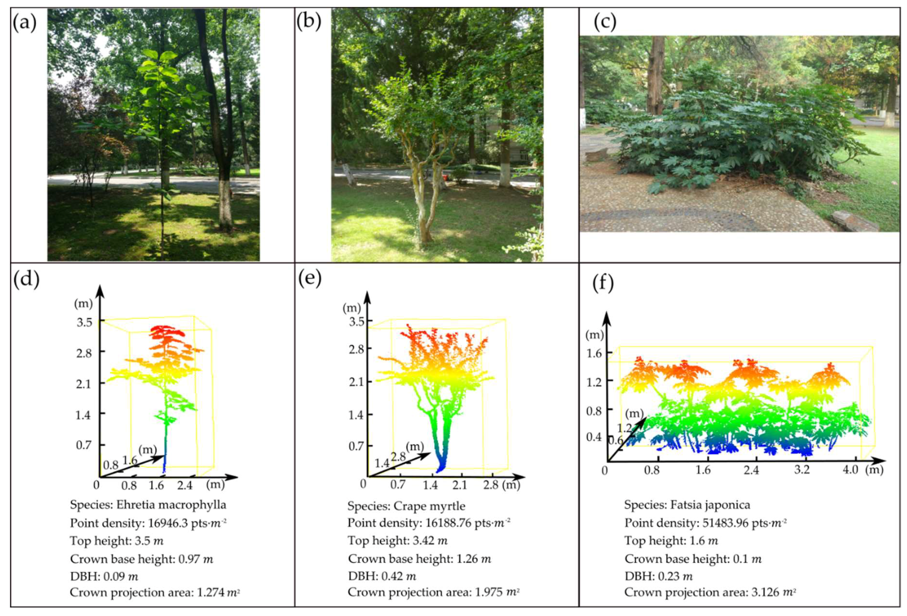
2.1. Study Site and Data Collection

The experimental trees were selected on the campus of Nanjing Forestry University (32°08’N, 118°81’E, WGS-84) and included many well-isolated individual Ehretia macrophylla (Ehretia macrophylla Wall), crape myrtle (Lagerstroemia indica L) and Fatsia japonica (Fatsia japonica (Thunb.) Decne. et Planch.) trees. All object trees with broad leaves and canopies with varying densities were scanned using a TLS (Leica C10) instrument, and one side-lateral scan was used to obtain the data.

The data were collected with a Leica C10 TLS system on May 2018. The Leica C10 instrument is a 532-nm phase-based scanner with a 360° × 270° upward field-of-view and laser rate of 50,000 points per second. The range measurement accuracy is ±1.5 mm at a distance of 3 m. The circular laser beam diameter and beam divergence at the scanner exit are 3 mm and 0.22 mrad, respectively, yielding a minimum distance between consecutive beams of approximately 0.4 mm at a distance of 3 m from the instrument. For the Ehretia macrophylla, crape myrtle and Fatsia japonica trees, the distances of the experimental trees and TLS were 5 m, 5 m and 3 m respectively, depending on tree height, in order to get the phenotypic characteristics of the whole tree in one scan within the viewing window. The height of the scanner was 1.57 m, 1.5 m and 0.8 m respectively. In this study, the normal scanning precision of the Leica C10 instrument was employed.

Three experimental trees, i.e., one Ehretia macrophylla, one crape myrtle and one Fatsia japonica tree, were selected for testing. Their structures represented by TLS point clouds are illustrated in Figure 1. The structural features of these trees, specifically tree height, crown base height and canopy projection area are listed in Figure 1. The LiDAR point density values were 16,946.3 points $\left(\mathrm{pts}\right)\cdot {\mathrm{m}}^{-2}$, 16,188.76 $\mathrm{pts}\cdot {\mathrm{m}}^{-2}$ and 51,483.96 $\mathrm{pts}\cdot {\mathrm{m}}^{-2}$ for the Ehretia macrophylla, crape myrtle and Fatsia japonica trees, respectively; the heights of the trees were 3.5 m, 3.42 m and 1.6 m respectively; the crown base heights of the trees were 0.97 m, 1.26 m and 0.1 m, respectively; the projected areas of the crowns were 1.274 ${\mathrm{m}}^2$, 1.975 ${\mathrm{m}}^2$ and 3.126 ${\mathrm{m}}^2$, respectively. The diameter at breast height (DBH) statistics for the trees are also listed in Figure 1, where DBH is defined as the sum of the diameter of each branch chest height. These comparisons indicate that the basic structural parameters of the sample trees were similar among all three tree species. Overall, there were no extreme cases of falling leaves and noise point increases due to the occurrence of strong winds for the selected trees. Thus, the selected experimental trees were appropriate for leaf attribute estimation.

To obtain the true leaf area and leaf angle distributions and demonstrate the validity of our method, the single-leaf area and leaf inclination and azimuthal angle of all target trees were measured using an LI-3000C portable area metre and angle measurement device. To validate the final results, we sampled the three experimental trees with different leaf numbers and manually measured the leaf inclination and azimuthal angles of all their leaves using an angle measurement device. For each experimental tree, the number of sampled leaves accounted for 40% of the total number of leaves in the crown, and the randomly sampled leaves were evenly distributed in the crown. Taking Ehretia macrophylla as an example, the crown was divided into upper, middle and lower portions. Each portion was divided into the eastern, western, northern and southern parts. Then, the tree crown was divided into 12 parts, with the sampled leaves distributed evenly in each part. The leaf angle distribution box plots (see Figure 2) show that the analytic dataset accounted for 40% of the total number of leaves in the tree crown, and the leaf inclination angle and leaf azimuth angle values tended to be relatively stable.

2.2. Wood-leaf Separation

Wood-leaf separation, which aims to classify LiDAR points into wood and leaf components, is an essential prerequisite for achieving leaf separation and deriving individual tree leaf characteristics. An unknown degree of wood components likely causes errors in leaf area estimates [55]. Considering the importance of wood-leaf separation results, in the current study, a series of features for each point [53] was used to separate the leaves of the experimental trees. These features were the normal vector, the structure tensor and the distribution of the point normal vector. Figure 3 shows the wood-leaf separation results, including the wood points and the leaf points for each of the three experimental trees.

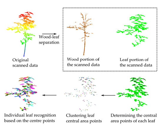
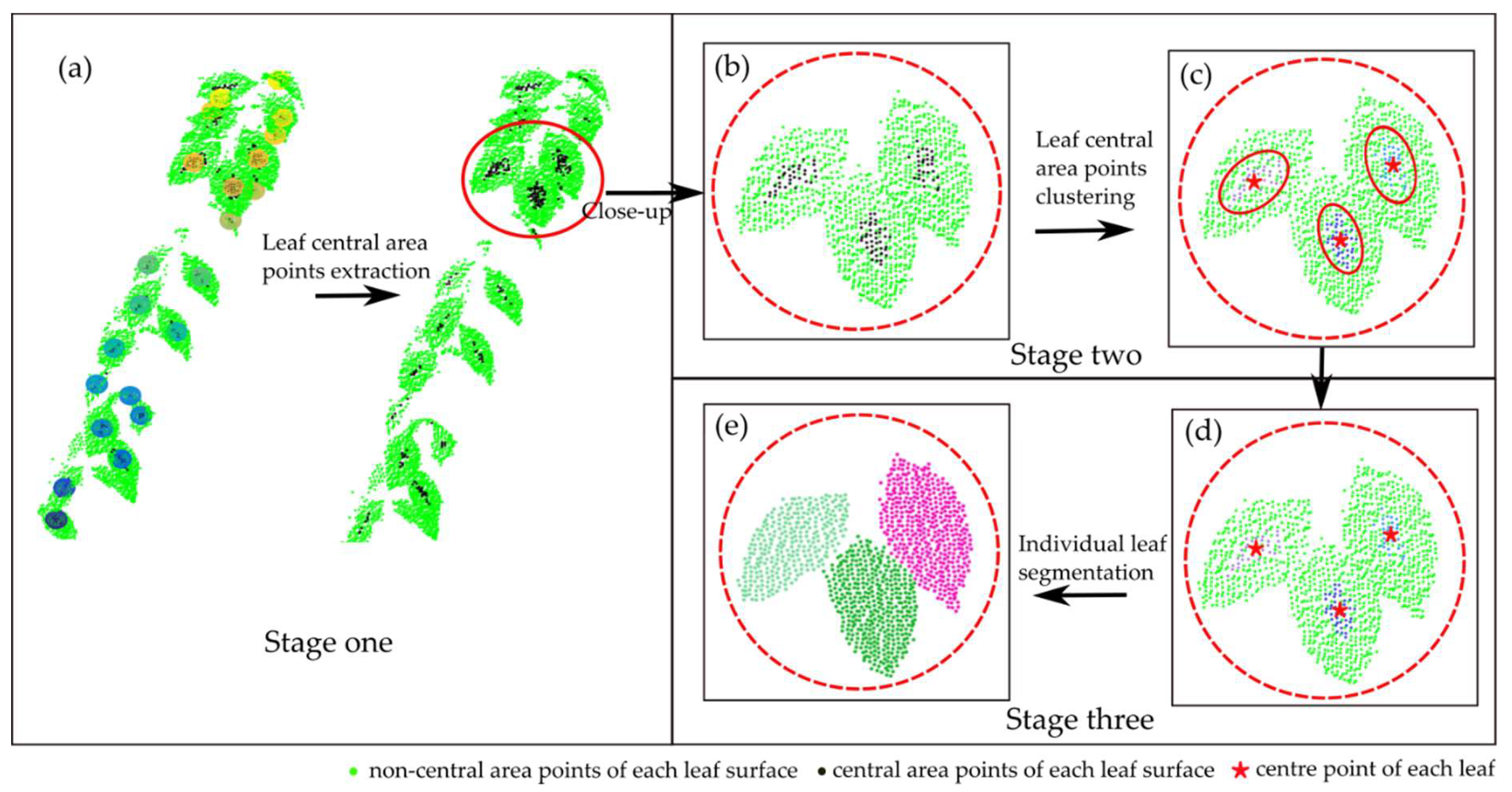
2.3. Individual Leaf Segmentation

The leaf blade is the main part of the tree crown and is mostly a green flat body with a large surface area, which is conducive to gas exchange and the absorption of light energy; this is of great relevance for studying leaf structure parameters. The sizes and shapes of leaves vary with different tree species. However, leaf morphology is relatively stable among leaves in the same plant and can be used as a basis for identifying plant species and individual leaf segmentation. The leaf blade width of the same plant has a relatively stable numerical range. The leaves of the three experimental trees studied in this paper have plane features; therefore, the corresponding scanned points of each leaf also have plane features.

Based on the above features, the proposed algorithm of individual leaf segmentation consists of three main stages, which are shown in Figure 4. The first stage is the extraction of the point clouds of the leaf central with a sphere neighbourhood model with an adaptive radius; four auxiliary criteria are defined to ensure the accuracy of the extracted central area points of each leaf surface. In the second stage, the density-based spatial clustering of applications with noise algorithm (DBSCAN) is used to cluster the central area points of the leaves, thereby obtaining the centre point corresponding to each leaf surface. In the third stage, individual leaf segmentation is realized by an advanced leaf blade segmentation algorithm combined with a 3D watershed algorithm.

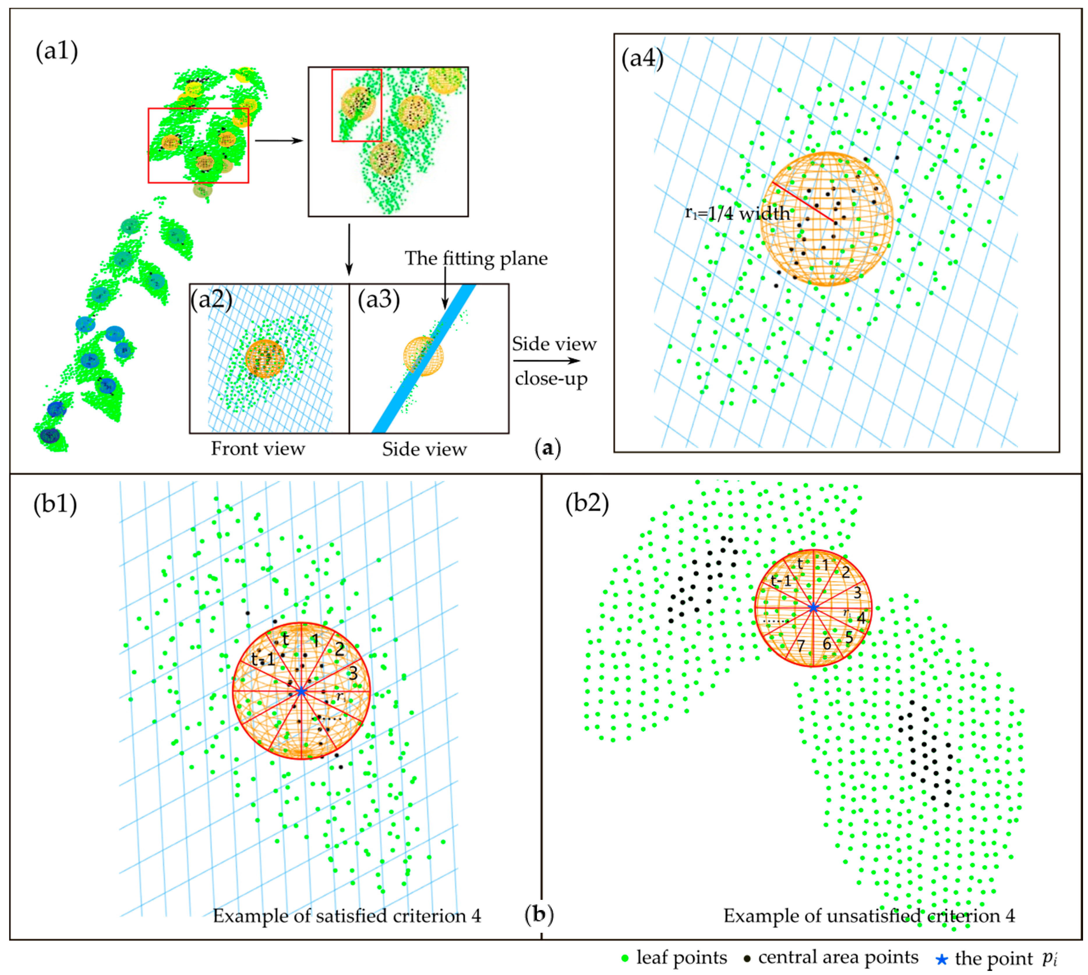
2.3.1. Extracting the Central Area Points of Individual Leaves

For leaves of different morphological structures and complex spatial distributions, it is especially important to determine the spatial plane where each leaf blade is located. Through analysis, the leaves of the three experimental trees can be approximately treated as a surface, and each leaf has its own centre point, which is usually at the centre of the leaf. However, each leaf has a different zenith angle and azimuth angle, making it difficult to directly express the plane of each leaf. However, central points must be able to extend in a certain spatial direction across the entire leaf blade to form a plane, which can always be found in 3D space, that is, the plane where the point cloud of the leaf blade is located. In the sphere neighbourhood model of the adaptive radius proposed in this paper, when the leaf blade point cloud uniformly fills the great circle plane in the whole sphere model, the centre of the sphere is the central area point of the leaf. Randomly distributed scanned points lie on a plane in 3D space on each leaf surface. The ternary equation $S_{\zeta }\left(x,y,z\right)=0$ is applicable to this situation, and any point $p_i\left(x_i,y_i,z_i\right),\left(i=1,2,3,\dots ,n_1\right)$ on the leaf blade satisfies $p_i\left(x_i,y_i,z_i\right)\in S_{\zeta },\left(\zeta =1,2,3,\dots ,n_2\right)$. $n_1$ represents the total number of scanned points in each tree crown. $n_2$ represents the total number of leaves in each tree crown, and the value of $n_2$ is unkown. $S_{\zeta }$ represents each leaf surface in 3D space. However, each leaf surface is irregular and cannot be easily expressed by a mathematical equation. To present the surface equation for each leaf, $S_{\zeta }$ can be represented by the central area points of each leaf surface. The extraction of points in the centre area of each leaf is also the basis for the subsequent individual leaf segmentation. Therefore, this paper primarily uses the sphere neighbourhood model to extract the central area points of each leaf, as shown in Figure 5a.

From the above analysis, each leaf blade is approximately in the plane distribution, and for the central area points of each leaf, the neighbourhood points must be uniformly distributed on a certain great circle of the sphere neighbourhood model. This paper defines four auxiliary criteria, and a point $p_i\left(x_i,y_i,z_i\right)$ that satisfies these auxiliary criteria is a leaf central area point. The point-to-point verification method is used to extract the centre area points of each leaf.

In this study, the extraction of leaf central area points by the point-to-point through the sphere neighbourhood model is the key step in individual leaf segmentation. First, the following variables must be defined: the radius of each sphere neighbourhood model is $r_1$, and the centre of each sphere is $p_i$, as shown in Figure 5(a4). The determination of the sphere neighbourhood model radius $r_1$ is a critical step in the pointwise classification because this variable can affect the classification accuracy. In this paper, the radius of the searching ball was set to $r_1=W_{tree}/4$ based on our sensitivity analysis to balance the classification accuracy and computational efficiency. $W_{tree}$ represents the average leaf width in the whole tree crown of the current process tree. For a point $p_i\left(x_i,y_i,z_i\right)$ in the point cloud $\mathrm{P},\mathrm{P}\subset R^3$, the neighbourhood points of $p_i$ within the radius $r_1$ were defined as $p_{i,j}\left(x_{i,j},y_{i,j},z_{i,j}\right)\left(j=1,2,3,\dots ,n_3\right)$ and satisfied the condition $p_{i,j}-p_i\le r_1$. $n_3$ is the number of neighbourhood points $p_{i,j}$ for the point $p_i$ (i.e., the number of points in the sphere neighbourhood model). The value of $n_3$ is should greater than $thresholds0$. The $thresholds0$ for the three experimental trees (Ehretia macrophylla, crape myrtle and Fatsia japonica) is set at 15, 10 and 30, respectively, according to the apparent characteristics of plants, leaf size and leaf area density.

$$\overline{p_i}=\frac{1}{n_3}{\displaystyle \sum }_{j=0}^{n_3}{p}_{i,j}$$

(1)

where $\overline{p_i}$ denotes the mean of the neighbourhood points $p_{i,j}$ for the point $p_i$.

Criterion 1:

Find the point $p_i$ that satisfies Equation (2). Equation (2) represents the distance between the current point $p_i$ and point $\overline{p_i}$, which is less than the $thresholds1$. Equation 2 ensures that the current point $p_i$ is close to its centre of the neighbourhood points.

$$\parallel p_i\overline{p_i}\parallel \ll thresholds1$$

(2)

Criterion 2:

Find the point $p_i$ that satisfies Equation (3). Equation (3) expresses that the current point $p_i$ must be close to the fitting plane $\overline{S_i}$. $\overline{S_i}$ is generated using the least squares method from the current point $p_i$ and its neighbourhood points $p_{i,j}$. The fitting plane is defined as $\overline{S_i}:A{x}_i+B{y}_i+C{z}_i+D=0$. The distance between the current point $p_i$ and the fitting plane $\overline{S_i}$ is less than $thresholds2$.

$$\frac{\left|A{x}_i+B{y}_i+C{z}_i+D\right|}{\sqrt{A^2+B^2+C^2}}<thresholds2$$

(3)

where the value of $thresholds2$ is half of the $thresholds1$ value.

Criterion 3:

Ensure that the distribution composed of the current point $p_i$ and its neighbourhood points has spatial planar features. Equation (4) guarantees that the distance between all the neighbourhood points $p_{i,j}$ of the current point $p_i$ and the fitting plane $\overline{S_i}$ are less than the $thresholds2$, which ensures that all the neighbourhood points $p_{i,j}$ are close to the fitting plane $\overline{S_i}$, i.e., the mean value of the distance from each neighbourhood point $p_{i,j}$ of the current point $p_i$ to the fitting $\overline{S_i}$ is less than the $thresholds2$.

$$\frac{1}{n_3}{\displaystyle \sum }_{j=1}^{n_3}\frac{\left|A{x}_{i,j}+B{y}_{i,j}+C{z}_{i,j}+D\right|}{\sqrt{A^2+B^2+C^2}}<thresholds2$$

(4)

where $n_3$ is the number of neighbourhood points $p_{i,j}$ for point $p_i$.

Criterion 4:

$S_i^c$ represents the great circle obtained by the intersection of the fitting plane $\overline{S_i}$ and the sphere neighbourhood model of the current point $p_i$, as shown in Figure 5(b1,b2). The great circle plane $S_i^c$ is divided into the $t$ block area as shown in Figure 5(b1,b2). The projection points of $p_i$ and $p_{i,j}$ on the great circle plane $S_i^c$ are $p_i^{\prime }$ and $p_{i,j}^{\prime }$, respectively. It is reasonable that the points $p_{i,j}^{\prime }$ should be uniformly distributed around point $p_i^{\prime }$ on the great circle plane $S_i^c$. The variation ratio is used to measure the degree by which the point $p_i^{\prime }$ and its neighbourhood points $p_{i,j}^{\prime }$ are distributed on the great circle plane $S_i^c$. $(Nu{m}_{p_{i,j}^{,}}-Nu{m}_v)/Nu{m}_{p_{i,j}^{,}}$ denotes the variation ratio of discrete points in each $v\left(v=1,2,\dots ,t\right)$ block area. $Nu{m}_{p_{i,j}^{,}}$ denotes the total number of projection points on the great circle plane, and $Nu{m}_v$ is the number of the projection points in the $vth$ block area Equation (5) guarantees that the point $p_i^{\prime }$ and its neighbourhood points $p_{i,j}^{\prime }$ are evenly distributed in each block area. This criterion eliminates candidate points at the leaf edge that overlap with other leaves, which can be mistakenly classified as the central area point (Figure 5(b1,b2)). The values of 0.6 and 1.4 are empirical values of individual leaf segmentation in our program.

$$0.6/t<Nu{m}_v/Nu{m}_{p_{i,j}^{,}}<1.4/t$$

(5)

Figure 5(b1) shows an example of satisfied criterion 4, and Figure 5(b2) shows an example of unsatisfied criterion 4.

The central area points $p_{\xi }^{carea}\left(\xi =1,2,3,\dots ,n_4\right)$ satisfying Equations (1)–(5) are extracted as black dots shown in Figure 5(a1). $n_4$ is the total number of central area points of each tree.

2.3.2. Clustering of Leaf Central Area Points

In real situations, the central area points of the leaves in each tree crown are divided into a large number of clusters. Therefore, we adopted the cluster algorithm proposed by Ester et al. [56], DBSCAN, to determine the central points of leaf segmentation. DBSCAN requires two input parameters containing the minimum number of points ($MinPts$) needed to form a cluster and the maximum radius of the neighbourhood from the core point ($MaxR$) (the maximum distance between clusters, here). The determination of the two input parameters is a critical step in the leaf central area points clustering process since these parameters can affect the accuracy of the clustering result. In this paper, the parameter $MinPts$ for the three experimental trees (Ehretia macrophylla, crape myrtle and Fatsia japonica) was set at 15, 10 and 30, respectively, according to the scanned point density and area of each leaf surface, which can be adopted to obtain the appropriate parameter $MaxR$ and achieve the classification result. The extracted data of the central area points of each leaf have a uniform distribution; then, $MaxR$ can be calculated from $MinPts$ and the size of the point cloud using the following equations [57]:

$$MaxR=\sqrt{\frac{T\cdot MinPts\cdot \Gamma \left[\left(1/2\right)\cdot n+1\right]}{n_4\sqrt{{\pi }^n}}}$$

(6)

$$T=\left[Max\left(x\left(p_{\xi }^{carea}\right)\right)-Min\left(x\left(p_{\xi }^{carea}\right)\right)\right]\left[Max\left(y\left(p_{\xi }^{carea}\right)\right)-Min\left(y\left(p_{\xi }^{carea}\right)\right)\right]\left[Max\left(z\left(p_{\xi }^{carea}\right)\right)-Min\left(z\left(p_{\xi }^{carea}\right)\right)\right]$$

(7)

where $n_4$ denotes the number of central area points of each tree crown. The value of n is 3 in this study, representing the dimensionality of the points. $\Gamma$ is the gamma function, and $T$ is the volume of the experimental space formed by m points. $p_{\xi }^{carea}$ denotes the data set of the central area points, and $x\left(p_{\xi }^{carea}\right),y\left(p_{\xi }^{carea}\right),z\left(p_{\xi }^{carea}\right)$ are the $x,y$ and $z$ values of $p_{\xi }^{carea}$, respectively.

$MaxR$ was obtained by Equation (6), calculated as half of the average leaf width for each tree crown. Then, the central area points were clustered based on the two input parameters $MaxR$ and $MinPts$. After the clustering analysis using the DBSCAN algorithm, the central area points of each leaf were segmented into different clusters, as shown by the coloured dots in Figure 4d. After the central area points $p_{\xi }^{carea}$ were divided into $n_2$ clusters, $p_{\xi ,k}^{carea}\left(\xi =1,2,3,\dots ,n_4,k=1,2,3,\dots ,n_2\right)$ was obtained to represent the central area points of each leaf blade surface, where $k$ indicates that the $\xi th$ centre area point belongs to the $kth$ cluster. The centre point for central area points $p_{\xi ,k}^{carea}$ of each leaf blade is denoted as $c_k\left(k=1,2,3\dots n_2\right)$ and is labelled by red stars in Figure 4d. $c_k$ represents the centre point of each leaf in the tree crown. These points serve as the seed point for the 3D watershed algorithm (Section 2.3.3). Each cluster of central area points $p_{\xi ,k}^{carea}$ corresponds to one centre point of each leaf $c_k$.

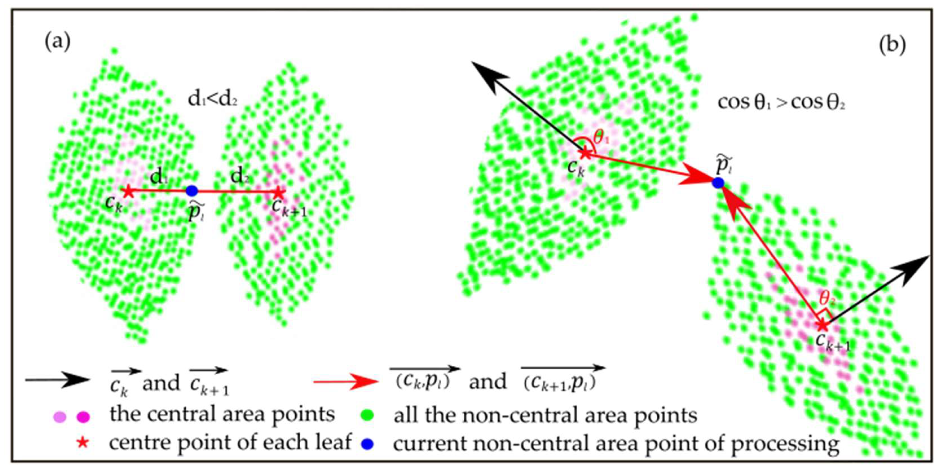
2.3.3. Individual Leaf Segmentation

The 3D watershed algorithm [58,59] is used to segment the remaining leaf point cloud of the tree crown, that is, the non-central area points $\widetilde{p_l}\left(l=1,2,3\dots n_5\right)$, where $\widetilde{p_l}{\displaystyle \cup }{p}_{\xi }^{carea}=p_i$. $n_5$ is the total number of non-central area points of each tree. In our method, the watershed algorithm starting points are the centre points of each leaf $c_k$, which were determined using our methods. The two morphology-related parameters, namely, the Euclidean distance between the centre point and the non-central area point and the cosine of the angle between the vector composed of the centre point and the non-central area point and the normal vector of the leaf blade, were used to segment individual leaves, which reduced the leaf oversegmentation problem and improved the precision of segmentation in the leaf edge detection. The ultimate goal of Equation (8) is to find the minimal value for each non-central area point $\widetilde{p_l}$, thereby completing the classification of each $\widetilde{p_l}$ value with the corresponding centre point $c_k$.

$$p_{l,k}^{leaf}=\mathrm{argmin}(a_1\parallel \widetilde{p_l}-c_k{\parallel }_2^2+a_2\cos (\angle (\overrightarrow{(c_k,\widetilde{p_l})},\overrightarrow{c_k})))$$

(8)

where $p_{l,k}^{leaf}\left(l=1,2,3\dots n_5,k=1,2,3\dots n_2\right)$ represents the point after classifying, as shown by coloured dots shown in Figure 4f. The first term on the right-hand side of equation $\parallel \widetilde{p_l}-c_k{\parallel }_2^2$ represents the Euclidean distance between the centre point $c_k$ and the non-centre point $\widetilde{p_l}$. The second term on the right-hand side of the equation $\cos (\angle (\overrightarrow{(c_k,\widetilde{p_l})},\overrightarrow{c_k}))$ calculates the cosine of the included angle between the vector composed of the centre point $c_k$ and the non-central area point $\widetilde{p_l}$ and the normal vector of the leaf blade surface $\overrightarrow{c_k}$. To balance the two terms, the parameters $a_1$ and $a_2$ should be adjusted. The equivalent relationship of the parameters $a_1$ and $a_2$ is $a_1+a_2=1$. In the experiment, the values of $a_1$ and $a_2$ were set to 0.7 and 0.3, respectively. Figure 6 illustrates Equation (8).

2.4. Leaf Attributes Calculation Based on Classified Leaf Points

After single-leaf segmentation via our method, Delaunay triangulation was adopted to deduce the area of each leaf. For segmented single-leaf scanning data, the normal vector of each leaf surface was obtained by fitting the leaf blade plane with the least squares method. For the known single-leaf point cloud data, the leaf inclination angle was used to calculate the included angle between the vector of the leaf surface normal and the zenith angle. According to the definition of the leaf azimuth angle, it is important to extract the principal axis of foliage. In this paper, the principal axis of each leaf blade is defined as the line between the most distant two points in a single-leaf point cloud. Thus, the leaf azimuthal angle can be obtained by calculating the clockwise angle between the north direction and the projection of the principal axis of foliage on the horizontal plane.

3. Results

3.1. Plant Leaf Classification

After applying our classification method to the preliminary scanned datasets of the experimental trees, we acquired an excellent consistency between the point clouds and real plant dimensions. These good results can be largely attributed to the proper selection of features, including the normal vector, the structure tensor and the distribution of the point normal vector. The quantitatively assessed classification accuracies of each target tree class are listed in

Table 1. Overall accuracy assessment of the classification of different tree species.

Tree Species	Ehretia Macrophylla	Crape Myrtle	Fatsia Japonica
Total number of points	36,604	107,914	247,133
Tree height (m)	3.5	3.42	1.6
Crown projection area (m2)	1.274	1.975	3.126
Average spatial sampling (cm)	0.55	0.45	0.42
Leaf point number (classified/actual)	27,841/29,387	72,639/78,564	184,721/201,648
Branch point number (classified/actual)	8763/7217	35,275/29,350	62,412/45,485
Overall accuracy	94.73%	92.46%	91.61%

. The tree height is a field measurement. The crown projection area is calculated by convex hull algorithms [60] of the single trees based on the scanned points. One result for leaf point number and the branch point number is obtained by the wood-leaf separation method in this study and the other using the manual measurement results. The overall accuracy is the ratio of the results produced by the classification method in this paper to the benchmark results derived using manual measurements.

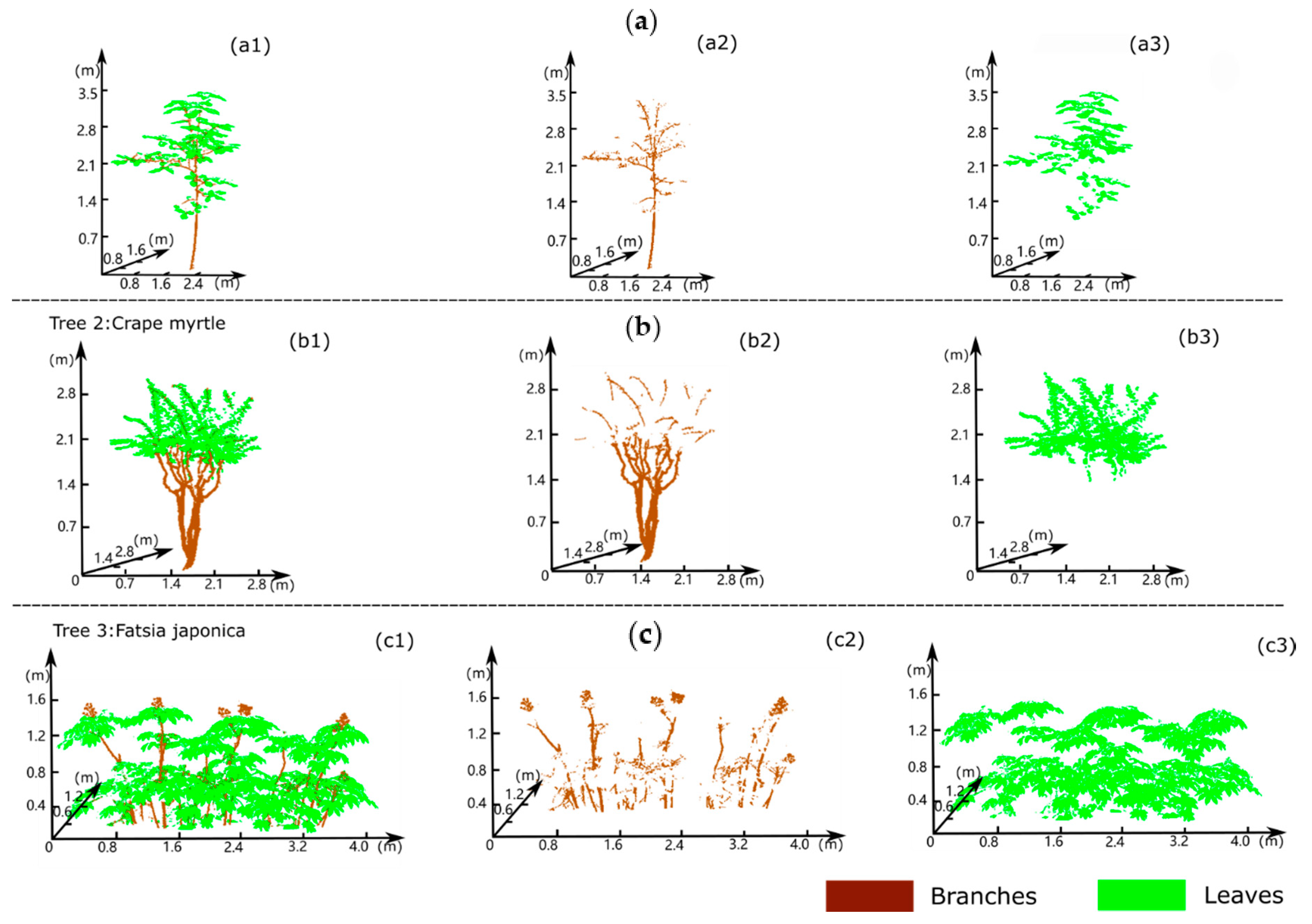
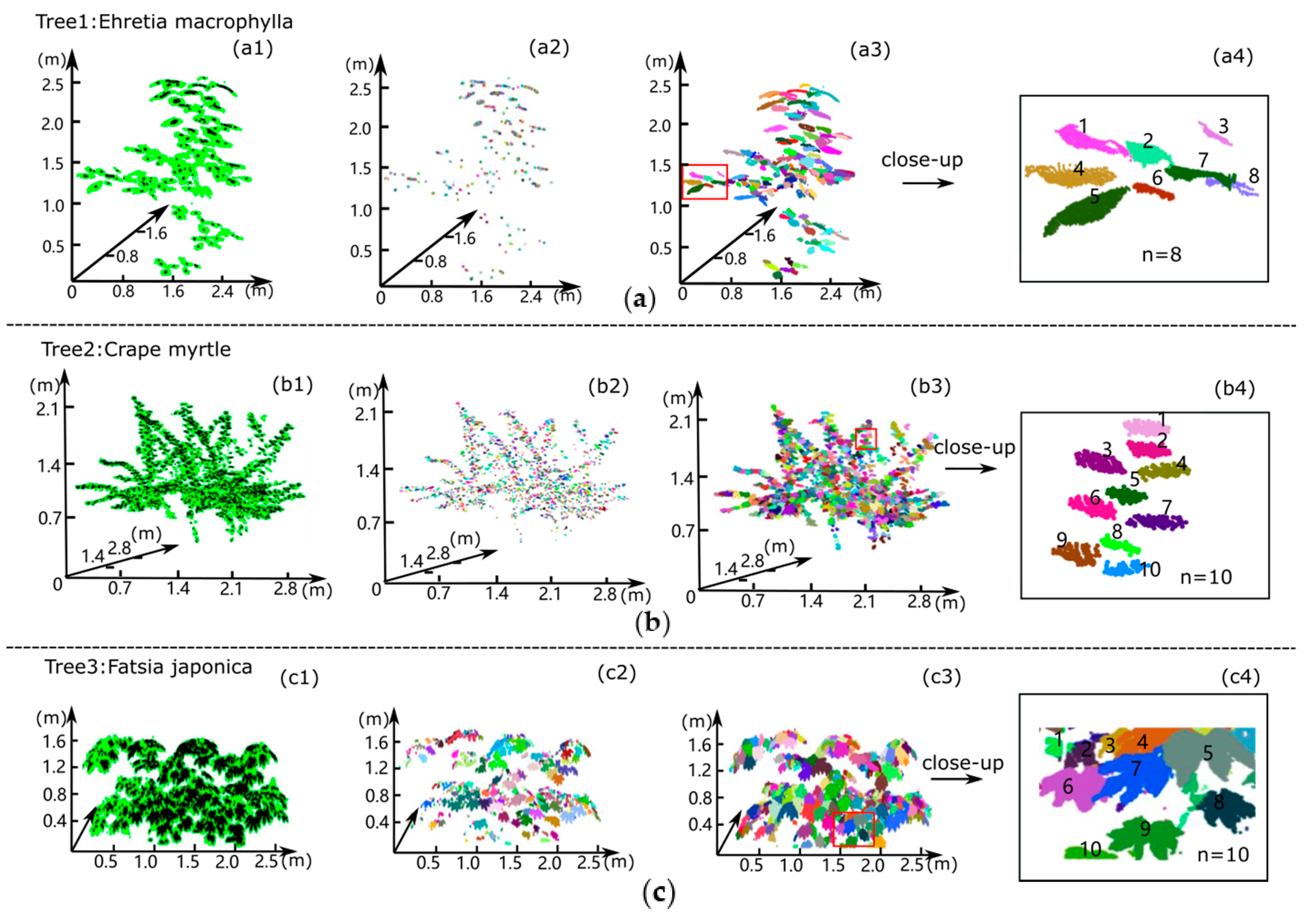
3.2. Leaf Segmentation

Three experimental trees were segmented using our method. The detailed results are shown in Figure 7 and demonstrate the classification results for Ehretia macrophylla (Figure 7a), crape myrtle (Figure 7b) and Fatsia japonica (Figure 7c). The accuracy of leaf segmentation is 94.0%, 90.6% and 88.8% for the Ehretia macrophylla, crape myrtle and Fatsia japonica trees, respectively. The accuracy of leaf segmentation in the upper tree crown (97.7%) was found for the Ehretia macrophylla trees than for the middle tree crown (90.6%) and lower tree crown (93.1%). The accuracy of leaf segmentation in the upper tree crown (92.2%) than for the lower tree crown (88.8%) was found for the crape myrtle trees. The central area points of each leaf for the experimental trees were accurately extracted by our method, and the extraction results are shown as black dots in Figure 7(a1,b1,c1). Then, the extracted central area points of the experimental trees were clustered using the DBSCAN algorithm, and the central area points of individual leaves were segmented into different clusters, as shown by the coloured dots in Figure 7(a2,b2,c2). The best segmentation effect was obtained for Ehretia macrophylla, which has relatively flat leaves in the overall canopy and an occlusion effect that is not obvious. The second best results were obtained for crape myrtle, which has a small leaf size and high leaf density; this tree type also achieved a good segmentation effect. Finally, Fatsia japonica, with the most complicated blade shape structure, also had a good segmentation effect.

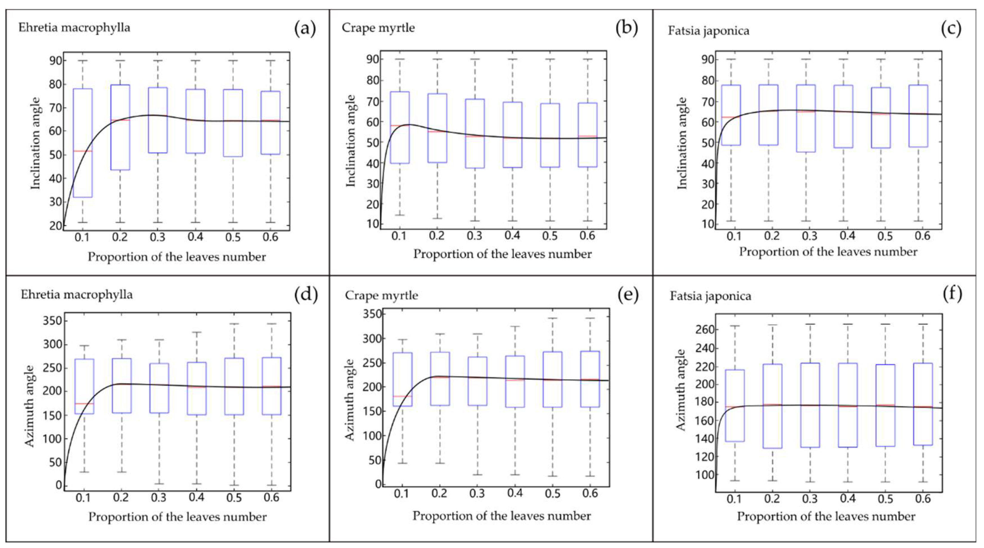
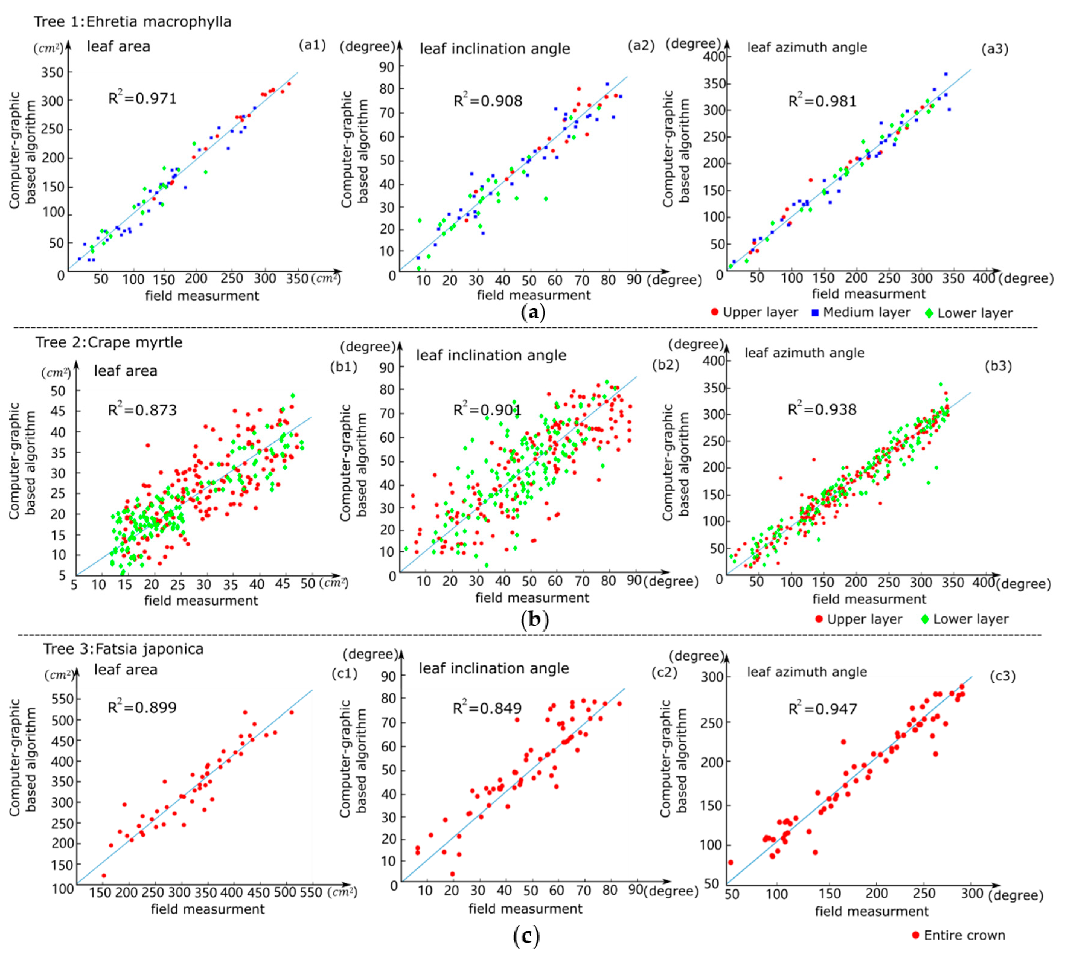
3.3. Leaf Attribute Calculation

After segmentation via our method, Ehretia macrophylla was divided into upper, middle and lower sections with three different horizontal layers, crape myrtle was divided into upper and lower sections with 2 different horizontal layers, and Fatsia japonica was not stratified. The segmented leaf points in the crowns were used as preliminary data and were randomly chosen as the analytic dataset. For each target tree, the leaves in the analytic dataset were evenly distributed in four directions, east, west, north and south, and the number of leaves in the analytic dataset accounted for 40% of the total number of leaves in the crown of the target tree. In this study, Delaunay triangulation was adopted to estimate each designated leaf area, and vector angles were computed to obtain leaf azimuthal angle and leaf inclination angle values. The specific leaf parameters obtained (e.g., leaf length, leaf width, leaf area, leaf azimuthal angle and leaf inclination angle) using our methods for different tree species are listed in

Table 2. Statistics of leaf attributes estimate for the three individual trees using our method and manual measurement.

Tree Species	Ehretia Macrophylla			Crape Myrtle		Fatsia Japonica
	Upper	Middle	Lower	Upper	Lower	Tree Crown
NP	12,477	14,316	3438	35,028	37,639	103,177
PD (pts·m−2)	4320	6260	6531	5844	9410	51,484
NLUM/ NLMM	44/ 43	87/ 96	27/ 29	501/ 543	440/ 495	187/ 166
RELN	2.33%	9.38%	6.90%	7.73%	11.11%	12.65%
RELL	5.57%	3.48%	1.16%	1.75%	15.1%	1.44%
RELW	2.75%	10.85%	3.55%	0.55%	0.93%	0.93%
RELA	2.67%	6.98%	4.67%	2.26%	16.12%	7.7%
LIAUM/ LIAMM (°)	28.4–88.0/ 25.1–86.8	9.1–89.8/ 7.5–89.0	9.3–81.2/ 2.7–77.8	7.9–89.7/ 11.7–88.2	5.2–84.0/ 1.2–89.8	9.6–87.8/ 6.8–89.2
LAAUM/ LAAMM (°)	44.8–322.0/ 31.3–313.5	11.8–349.6/ 3.3–353.6	14.7–324.5/ 15.6–323.8	18.6–227.0/ 12.7–269.4	19.7–295.7/ 23.0–309.3	53.3–268.8/ 50.9–266.3

NP: number of points; PD: point density; NLUM: number of leaves using our method; NLMM: number of leaves from manual measurements; RELN: the ratio of error for the number of leaves; RELL: the ratio of error for the average leaf length; RELW: the ratio of error for the average leaf width; RELA: the ratio of error for the average leaf area; LIAUM: leaf inclination angle using our method; LIAMM: leaf inclination angle from manual measurements; LAAUM: leaf azimuth angle using our method; LAAMM: leaf azimuth angle from manual measurements.

. A comparison of the number of leaves in each crown obtained via manual measurements and using our method is presented in Table 2, which indicates that our method obtained satisfactory estimates of the number of individual tree leaves. Table 2 shows that the leaf areas determined by the Delaunay triangulation algorithm are very similar to the actual leaf areas obtained by manual measurements. In addition, the values of the angle distribution calculated directly on the point clouds were effectively highly correlated with the measurements of the actual angles taken in the field.

Figure 8 depicts the measured vs. estimated individual leaf attribute values, including leaf area, leaf azimuthal angle, and leaf inclination angle, obtained using our method and manual measurements. The leaf attribute estimations of the correctly detected trees using our method fall close to the 1:1 line on, the scatterplots of field-measured and method-estimated leaf attributes for cross-validation (Figure 8). The widths of the confidence intervals for Ehretia macrophylla are relatively narrow, indicating the high quality of Ehretia macrophylla’s leaf segmentation and attribute estimation result. In general, there were no significant mean differences between the field-measured and method-estimated values for leaf area, inclination and azimuthal angles (see

Table 3. Statistics for the overall results of the leaf morphological features (leaf area, leaf azimuthal angle and leaf inclination angle).

Tree species	Position	R2			RMSE
		LA	LIA	LAA	LA (cm2)	LIA (°)	LAA (°)
Ehretia macrophylla	Upper	0.987	0.894	0.990	8.805	5.686	7.709
	Middle	0.959	0.914	0.978	7.596	6.489	7.316
	Lower	0.888	0.831	0.982	9.357	7.841	8.151
	All	0.971	0.908	0.981	8.508	6.806	7.680
Crape myrtle	Upper	0.934	0.864	0.941	7.042	8.459	7.011
	Lower	0.801	0.905	0.934	4.579	8.260	8.180
	All	0.873	0.901	0.938	6.001	8.365	7.573
Fatsia japonica	All	0.899	0.849	0.947	5.744	6.158	3.946

LA: leaf area; LIA: leaf inclination angle; LAA: leaf azimuthal angle.

). This result indicated that the individual leaf area estimation was in good agreement with values obtained from actual measurements and that the individual leaf area in the upper tree crown was larger than that in the middle and lower tree crown (Figure 8(a1,b1)). The leaf inclination angle estimations were in good agreement with values obtained from actual measurements for the three experimental trees (${\mathrm{R}}^2$ = 0.908, RMSE = 6.806°, ${\mathrm{R}}^2$ = 0.901, RMSE = 8.365° and ${\mathrm{R}}^2$= 0.849, RMSE = 6.158°, respectively; Figure 8(a2,b2,c2)). A higher probability of large inclination angles in the upper crown was found for the Ehretia macrophylla and the crape myrtle trees than for the middle tree crown and lower tree crown (Figure 8(a2,b2)). One explanation for this result could be that upper crown leaves grow more vertically than lower crown leaves to increase the amount of solar radiation penetrating through the plant canopy, ultimately increasing the possibility of light penetration and benefiting the growth of lower foliage elements [23]. Similarly, lower leaf elements tend to grow more horizontally than upper leaf elements to optimize the absorbed solar radiation. The leaf azimuthal angles of the estimations were in good agreement with values obtained from actual measurements of the three experimental trees for Ehretia macrophylla, crape myrtle and Fatsia japonica. (${\mathrm{R}}^2$ = 0.981, RMSE = 7.680°, ${\mathrm{R}}^2$ = 0.938, RMSE = 7.573° and ${\mathrm{R}}^2$ = 0.947, RMSE = 3.946°, respectively; Figure 8 c1–(c3)). The variations in the leaf azimuthal angle distributions with tree height were very small. In the Ehretia macrophylla tree, leaf azimuthal angles were randomly distributed from 3.3° to 353.6° across the whole crown (Figure 8(a3)). The azimuthal angle distribution of the crape myrtle tree from the upper to lower layers was very similar (Figure 8(b3)). In addition, the Fatsia japonica azimuthal angle probability ranged from 50.9° to 266.3°, which might be attributed to the light source orientation of vegetation leaves or the incomplete data collection of the one side-lateral TLS (Figure 8(c3)). These findings demonstrate that the segmentation method allows the robust determination of the distribution of orientation values.

4. Discussion

For the optimization of plant cultivation, the monitoring of crop growth and productivity, successive leaf attribute measurements are necessary [61,62]. It is well established that leaf area is pivotal for light interception, photosynthesis and transpiration and leaf angle distribution is an important canopy structure parameter that has a great influence on the transmission of radiation within vegetation canopies and the distribution of incident photosynthetically active radiation [63,64]. Thus these features are key parameters in several agronomic and physiological studies [65,66,67]. TLS has emerged as among the most promising remote sensing technologies, providing detailed, spatially explicit, 3D information on plant structure, for operational applications in a wide range of disciplines related to the extraction of plant morphological features. These applications include, as reported in previous literature, the estimation of forest biophysical parameters such as gap fraction [68] and leaf area index [69,25]. These methods mostly aim to extract the vertical and horizontal distributions of biophysical variables or to determine an empirical correlation formula between laser scanning and in situ data sets. The literature [70,71] has reported that the non-photosynthetic and photosynthetic parts of trees should be separated to achieve more accurate biomass estimations. The specific analysis of the photosynthetic part of trees by TLS improves leaf area index estimations. Gaussian mixture models [72] are successfully used for separating leaf and non-leaf classes of individual trees, and a support vector machine classification technique [53] has been presented to extract the leaves of trees. On this basis, the leaf separation of the canopy was successfully achieved in the present study, and parameter analysis at the single-leaf scale was completed. The following points must be considered to apply this method to leaf segmentation and leaf attribute measurements.

4.1. Tree Species Effects

Tree species showed a negligible effect on the final classification accuracy using the proposed method. For the experimental trees, the final accuracy for Ehretia macrophylla was 94.0% (see Table 2), the final accuracy for crape myrtle was 90.6% (see Table 2) and the final accuracy for Fatsia japonica was 88.8% (see Table 2). The Fatsia japonica tree, with the most complicated blade shape structure, also had good segmentation results. The study results show that our method is not suitable for coniferous trees because it is difficult to determine the centre points of coniferous leaves by using sphere neighbourhood model, but the phenotypic traits of broad leaves with wide surfaces are suitable for our algorithms. Although different species have varying leaf inclination angles and leaf density distributions, resulting in different degrees of occlusion and the need for different search radii and thresholds to be set, our method can still provide a valuable and reasonable approach for assessing the real leaf area. However, for TLS, there are more occlusions and a greater lack of scanned data in the upper part of the tree crown in tall trees, which leads to low accuracy in the segmentation of individual leaves by the algorithm. We can consider the combination of airborne laser scanning (ALS) [73] and TLS scan modes to obtain complete scanned data and use the method proposed in this study to calculate each leaf attribute in the whole tree crown. Thus, our proposed method can accurately and efficiently detect individual tree leaves and their morphological attributes from scanned point cloud data.

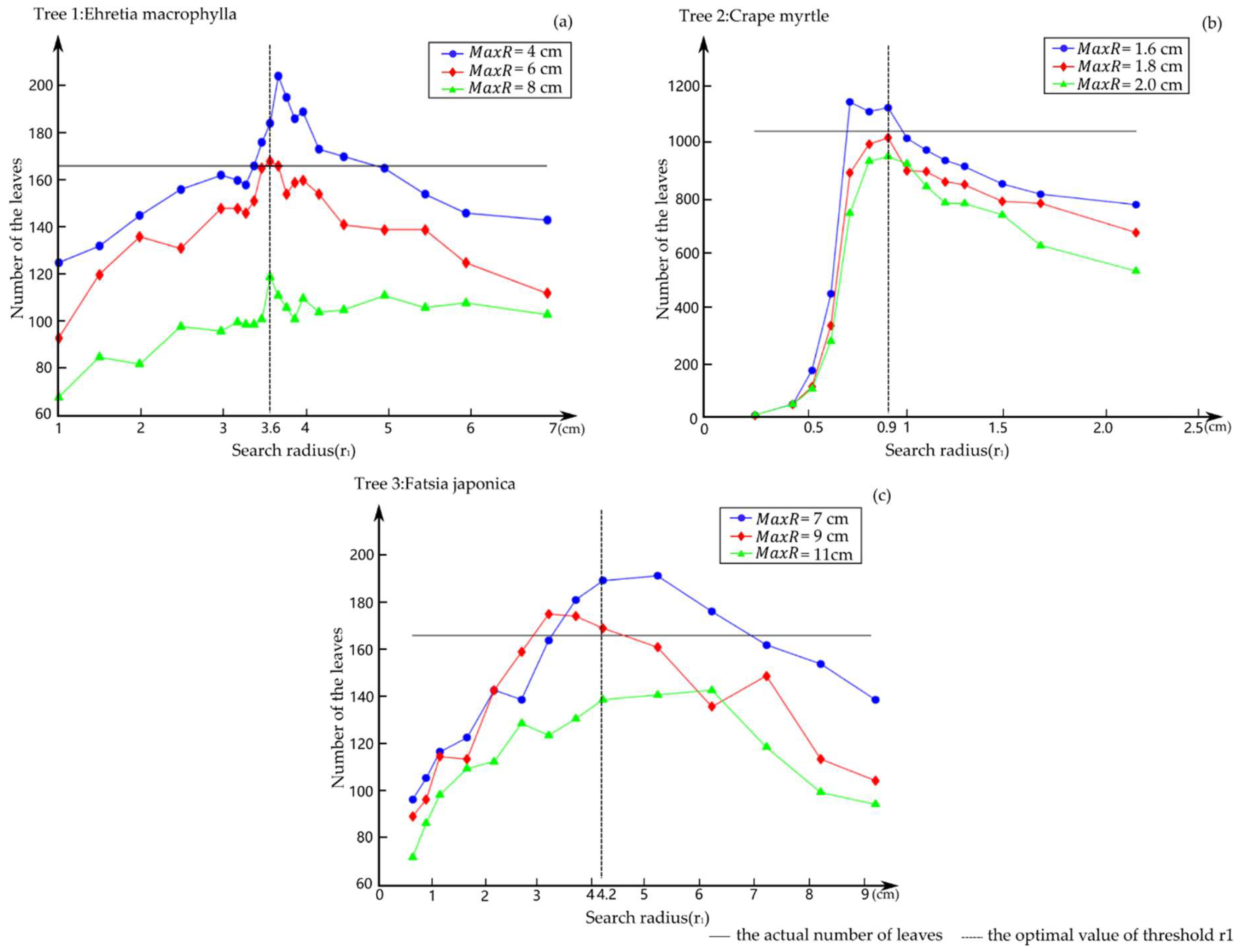
4.2. Sensitivity Analysis of Search Radius ($r_1$)

The search radius $r_1$ affected both the preliminary and final individual leaf segmentation results. To better understand the effect of the search radius $r_1$ on the central area point extraction accuracy, a sensitivity analysis was conducted using the data from the three experimental trees. The sensitivity analysis showed that the correctly segmented leaf number (CSLN) curves for all experimental tree crowns changed as the search radius increased. As shown in Figure 9, the CSLN increased as the search radius $r_1$ increased for all experimental trees. The highest individual leaf segmentation accuracy was obtained when the search radius $r_1$ reached 3.6 cm, 0.9 cm and 4.2 cm for Ehretia macrophylla, crape myrtle and Fatsia japonica, respectively. In this case, the values of search radius $r_1$ (3.6 cm, 0.9 cm and 4.2 cm) were approximately equal to one quarter of the average leaf width in each tree crown. The average widths of the leaves in the tree crown for Ehretia macrophylla, crape myrtle and Fatsia japonica were 12.8 cm, 3.6 cm and 17.2 cm, respectively; in addition, the CSLN for the experimental tree crowns provided increasingly lower segmentation accuracy when the search radius $r_1$ was greater than 3.6 cm, 0.9 cm and 4.2 cm, respectively. In the case in which the scanning precision remain unchanged, the shorter the search radius, the fewer the points in the sphere neighbourhood model. When the number of points in the sphere neighbourhood model was greater than the thresholds0 and the four auxiliary criteria (discussed in Section 2.3.1) defined were satisfied, the point $p_i$ satisfied the conditions to be considered the central area point of the leaf. Therefore, when the radius of the sphere neighbourhood model decreases, the number of points in the great circle plane will be decreased and the number of calculated central area points will be gradually reduced, resulting in a downtrend in the recognition of leaves using our program. The value of the input parameter $MaxR$ also affected the final individual leaf segmentation when leaf central area points were clustered using the DBSCAN algorithm. As shown in Figure 9, when the value of $MaxR$ was larger, the number of leaf blades segmented was smaller; when the value of $MaxR$ was smaller, the number of leaf blades segmented was larger. Overall, when the value of $MaxR$ was approximately half of the average leaf width in the tree crown, the results showed the highest segmentation accuracy (see Figure 9). The intersection of two lines for each figure in Figure 9 represents the optimal detected leaf number result, which is closest to the true value.

Our results suggest that for the three experimental trees, the CSLN changed as the search radius $r_1$ increased, and the highest segmentation accuracy was obtained when $r_1$ was one-quarter of the average width of the leaves of each tree crown. In addition, the best selected value of the input parameter $MaxR$ was approximately half of the average leaf width for the crowns of the different tree species.

4.3. Recommendations

The occlusion of forest trees is determined by various factors such as leaf area index, the location of the scanner, scanning parameter setting [74], brand of the scanner [75] and tree topological structure. These factors deserve further exploration. The TLS setup could affect the classification accuracy, and the TLS-measured data were scanned from one perspective which might cause the representation accuracy of the leaves to be relatively low and not homogeneous, with the shadow effect on the other side of the tree. Considering that the occlusion inside the tree crown of the three experimental trees in this study is not serious, only one-sided scanning was sufficient to obtain nearly overall information of the tree crown and acquire the corresponding high-density point cloud. Furthermore, the spatial resolution of the point clouds decreased as the acquisition distance between the TLS instrument and the experimental tree increased, causing leaves or branches to be misclassified and tree stems or branches surrounded by shrubs or grasses to often be misclassified as random leaf points. As a result, the wood-leaf separation and leaf point occlusion were greater, which reduced the leaf segmentation accuracy. Finally, the noise points caused by wind had a great influence on the leaf segmentation and the calculation of the area of individual leaves. Thus, it was very important to remove noise points for the direct estimation of individual leaf areas. To increase the accuracy of the segmentation of individual leaves, we recommend using multiple scan locations to better capture the 3D structural characteristics of experiment trees. In addition to the above factors, the quality of the point cloud data (including accuracy and completeness) was another important factor that increased the algorithm accuracy of single leaf blade segmentation. The low segmentation precision rate for the leaf blade in the TLS-based data was primarily caused by the incompleteness of the wood-leaf separation. The quality of the TLS-based data was affected by three factors: outliers, woody phytoelement points, and occlusion. Although we removed outliers and woody phytoelement points, the influence of these three factors could not be completely eliminated. The quality of the TLS-based data still has room to improve. Therefore, the need to achieve better denoising and the separation of woody points from foliage points represents a great challenge to accurate leaf segmentation in future studies.

Our method’s final individual leaf segmentation accuracy increased as the occlusion of the tree crown decreased. The results showed that the leaf recognition ratio decreased for TLS-based data as the leaf numbers and point cloud density increased (see Table 2). This phenomenon could be explained by the fact that the degree of overlapping in the leaf distribution increased as the leaf number increased, and a high degree of leaf overlapping increased the difficulty of leaf segmentation and decreased the leaf recognition ratio. The individual leaf segmentation accuracy was as low as 88.80% for Fatsia japonica, which was characterized by a high point cloud density (51,483.96 $\mathrm{pts}\cdot {\mathrm{m}}^{-2}$). Among the three experimental trees, Fatsia japonica showed the lowest final leaf segmentation accuracy. This result was likely due to the more severe occlusion within the tree crown, leading to the incomplete wood-leaf separation, and the complicated leaf blade shape structure inherent in Fatsia japonica. In the case of the crape myrtle, which was characterized by a medium point cloud density (16,188.76 $\mathrm{pts}\cdot {\mathrm{m}}^{-2}$), the individual leaf segmentation was as high as 93.62%. The leaf segmentation accuracy of the crape myrtle in two different horizontal layers was also negatively correlated with point density (see Table 2). Finally, for Ehretia macrophylla, which was characterized by a low point cloud density (16,946.3 $\mathrm{pts}\cdot {\mathrm{m}}^{-2}$), the final individual leaf segmentation reached up to 94.0%. For the upper, middle and lower layers of the Ehretia macrophylla tree, which represented three different horizontal layers, the internal occlusion and point density of the upper tree crown were lower than those of the other layers, so the individual leaf segmentation accuracy was the highest; the middle tree crown had the highest number of leaves, and the individual leaf segmentation accuracy of the middle layer was slightly lower than the segmentation accuracy of the other layers of the tree crown (see Table 2).

5. Conclusions

This study developed a computer graphic-based 3D point cloud segmentation approach for accurately and efficiently detecting tree leaves and their morphological features, including leaf area, leaf azimuthal angle and leaf inclination angle, from individual leaves. First, based on the proposed computer graphics methods, the sphere neighbourhood model with an adaptive radius was used to extract the central area points of each leaf blade. In addition, four auxiliary criteria were defined to ensure the accuracy of the extracted central area points of each leaf surface. Second, DBSCAN was used to cluster the central area points of individual leaves. Third, based on the extracted centre point of each leaf combined with the advanced 3D watershed algorithm, individual leaf segmentation was achieved. Finally, leaf morphological features (leaf area and leaf angle distributions) were calculated from the single-leaf point cloud data of the segmented leaves to derive single-leaf-scale information and investigate the usability of leaf segmentation.

The results demonstrated that the segmentation accuracy for Ehretia macrophylla (94.0%) was higher than that for crape myrtle (90.6%) and Fatsia japonica (88.8%). The segmentation accuracy for Fatsia japonica was the lowest of the three experimental trees. Second, the single-leaf area estimation accuracy was the highest for Ehretia macrophylla (95.39%), and the single-leaf area estimation accuracy for crape myrtle (91.92%) was lower than that for Ehretia macrophylla (95.39%) and Fatsia japonica (92.48%). Third, the method proposed in this paper provided accurate leaf inclination and azimuthal angles for three experimental trees (Ehretia macrophylla: leaf inclination angle: ${\mathrm{R}}^2$ = 0.908, RMSE = 6.806° and leaf azimuth angle: ${\mathrm{R}}^2$ = 0.981, RMSE = 7.680°; crape myrtle: leaf inclination angle: ${\mathrm{R}}^2$ = 0.901, RMSE = 8.365° and leaf azimuth angle: ${\mathrm{R}}^2$ = 0.938, RMSE = 7.573°; Fatsia japonica: leaf inclination angle: ${\mathrm{R}}^2$= 0.849, RMSE = 6.158° and leaf azimuth angle: ${\mathrm{R}}^2$ = 0.947, RMSE = 3.946°). Our method provides a novel method for appraising individual leaf-scale information including leaf area and leaf angle distributions and has promising potential for more accurate biomass, or LAI calculation and for analysing vegetation structure.

References

1. Han, W.T.; Sun, Y.; Xu, T.F.; Chen, X.W.; Su, K.O. Detecting maize leaf water status by using digital RGB images. Int. J. Agric. Biol. Eng. 2014, 7, 45–53. [Google Scholar] [CrossRef]
2. Harley, P.C.; Baldocchi, D.D. Scaling carbon dioxide and water vapour exchange from leaf to canopy in a deciduous forest. I. Leaf model parametrization. Plant Cell Environ. 2010, 18, 1146–1156. [Google Scholar] [CrossRef]
3. Huang, J.; Sedano, F.; Huang, Y.; Ma, H.; Li, X.; Liang, S.; Tian, L.; Zhang, X.; Fan, J.; Wu, W. Assimilating a synthetic Kalman filter leaf area index series into the WOFOST model to improve regional winter wheat yield estimation. Agric. For. Meteorol. 2016, 216, 188–202. [Google Scholar] [CrossRef]
4. Strebel, D.E.; Goel, N.S.; Ranson, K.J. Two-Dimensional Leaf Orientation Distributions. IEEE Trans. Geosci. Remote Sens. 1985, 23, 640–647. [Google Scholar] [CrossRef]
5. Ross, J. The Radiation Regime and Architecture of Plant Stands; Springer: Cham, The Netherlands, 1981. [Google Scholar] [CrossRef]
6. Lugg, D.G.; Youngman, V.E.; Hinze, G. Leaf Azimuthal Orientation of Sorghum in Four Row Directions. Agron. J. 1981, 73, 497–500. [Google Scholar] [CrossRef]
7. Chianucci, F.; Cutini, A.; Corona, P.; Puletti, N. Estimation of leaf area index in understory deciduous trees using digital photography. Agric. For. Meteorol. 2014, 198–199, 259–264. [Google Scholar] [CrossRef]
8. Peper, P.J.; Mcpherson, E.G. Evaluation of four methods for estimating leaf area of isolated trees. Urban For. Urban Green. 2004, 2, 19–29. [Google Scholar] [CrossRef]
9. Colaizzi, P.D.; Evett, S.R.; Brauer, D.K.; Howell, T.A.; Tolk, J.A.; Copeland, K.S. Allometric Method to Estimate Leaf Area Index for Row Crops. Agron. J. 2017, 109. [Google Scholar] [CrossRef]
10. Xie, D.; Wang, Y.; Hu, R.; Chen, Y.; Yan, G.; Zhang, W.; Wang, P. Modified gap fraction model of individual trees for estimating leaf area using terrestrial laser scanner. J. Appl. Remote Sens. 2017, 11. [Google Scholar] [CrossRef]
11. Macfarlane, C.; Ryu, Y.; Ogden, G.N.; Sonnentag, O. Digital canopy photography: Exposed and in the raw. Agric. For. Meteorol. 2014, 197, 244–253. [Google Scholar] [CrossRef]
12. Stenberg, P. Correcting LAI-2000 estimates for the clumping of needles in shoots of conifers. Agric. For. Meteorol. 1996, 79, 1–8. [Google Scholar] [CrossRef]
13. Chen, J.M.; Cihlar, J. Quantifying the effect of canopy architecture on optical measurements of leaf area index using two gap size analysis methods. IEEE Trans. Geosci. Remote Sens. 1995, 33, 777–787. [Google Scholar] [CrossRef]
14. Yun, T.; Li, W.; Sun, Y.; Xue, L. Study of Subtropical Forestry Index Retrieval Using Terrestrial Laser Scanning and Hemispherical Photography. Math. Probl. Eng. 2015, 2015, 206108. [Google Scholar] [CrossRef]
15. Mason, E.G.; Diepstraten, M.; Pinjuv, G.L.; Lasserre, J.P. Comparison of direct and indirect leaf area index measurements of Pinus radiata D. Don. Agric. For. Meteorol. 2012, 166–167, 113–119. [Google Scholar] [CrossRef]
16. Asner, G.P.; Scurlock, J.M.O.; Hicke, J.A. Global synthesis of leaf area index observations: Implications for ecological and remote sensing studies. Glob. Ecol. Biogeogr. 2010, 12, 191–205. [Google Scholar] [CrossRef]
17. Zhao, K.; García, M.; Liu, S.; Guo, Q.; Chen, G.; Zhang, X.; Zhou, Y.; Meng, X. Terrestrial lidar remote sensing of forests: Maximum likelihood estimates of canopy profile, leaf area index, and leaf angle distribution. Agric. For. Meteorol. 2015, 209–210, 100–113. [Google Scholar] [CrossRef]
18. Ali, A.M.; Darvishzadeh, R.; Skidmore, A.K.; van Duren, I. Specific leaf area estimation from leaf and canopy reflectance through optimization and validation of vegetation indices. Agric. For. Meteorol. 2017, 236, 162–174. [Google Scholar] [CrossRef]
19. Norman, J.M.; Campbell, G.S. Canopy Structure-in Plant Physiological Ecology: Field Methods Instrumentation; Chapman and Hall: London, UK, 1989; pp. 301–325. [Google Scholar]
20. Lang, A.R.G. Leaf orientation of a cotton plant. Agric. Meteorol. 1973, 11, 37–51. [Google Scholar] [CrossRef]
21. Zou, X.; Mõttus, M. Retrieving crop leaf tilt angle from imaging spectroscopy data. Agric. For. Meteorol. 2015, 205, 73–82. [Google Scholar] [CrossRef]
22. Pisek, J.; Ryu, Y.; Alikas, K. Estimating leaf inclination and G-function from leveled digital camera photography in broadleaf canopies. Trees 2011, 25, 919–924. [Google Scholar] [CrossRef]
23. Raabe, K.; Pisek, J.; Sonnentag, O.; Annuk, K. Variations of leaf inclination angle distribution with height over the growing season and light exposure for eight broadleaf tree species. Agric. For. Meteorol. 2015, 214–215, 2–11. [Google Scholar] [CrossRef]
24. Daughtry, C.S.T. Direct measurements of canopy structure. Remote Sens. Rev. 1990, 5, 45–60. [Google Scholar] [CrossRef]
25. Zheng, G.; Moskal, L.M.; Kim, S.H. Retrieval of Effective Leaf Area Index in Heterogeneous Forests With Terrestrial Laser Scanning. IEEE Trans. Geosci. Remote Sens. 2013, 51, 777–786. [Google Scholar] [CrossRef]
26. Bayer, D.; Seifert, S.; Pretzsch, H. Structural crown properties of Norway spruce (Picea abies L. Karst.); and European beech (Fagus sylvatica L.) in mixed versus pure stands;revealed by terrestrial laser scanning. Trees 2013, 27, 1035–1047. [Google Scholar] [CrossRef]
27. Wezyk, P.; Koziol, K.; Glista, M.; Pierzchalski, M. Terrestrial laser scanning versus traditional forest inventory first results from the polish forests. In Proceedings of the ISPRS Workshop on Laser Scanning, 12–14 September 2007, Espoo, Finland.
28. Liu, G.; Wang, J.; Dong, P.; Chen, Y.; Liu, Z. Estimating Individual Tree Height and Diameter at Breast Height (DBH) from Terrestrial Laser Scanning (TLS) Data at Plot Level. Forests 2018, 9, 398. [Google Scholar] [CrossRef]
29. Zheng, G.; Moskal, L.M. Retrieving Leaf Area Index (LAI) Using Remote Sensing: Theories, Methods and Sensors. Sensors 2009, 9, 2719–2745. [Google Scholar] [CrossRef] [Green Version]
30. Hosoi, F.; Nakai, Y.; Omasa, K. Estimating the leaf inclination angle distribution of the wheat canopy using a portable scanning lidar. Agric. Meteorol. 2009, 65, 297–302. [Google Scholar] [CrossRef] [Green Version]
31. Janowski, A.; Bobkowska, K.; Szulwic, J. 3D modelling of cylindrical-shaped objects from lidar data—An assessment based on theoretical modelling and experimental data. Metrol. Meas. Syst. 2018, 25, 47–56. [Google Scholar]
32. Janowski, A. The circle object detection with the use of Msplit estimation. E3S Web Conf. 2018, 26, 00014. [Google Scholar] [CrossRef] [Green Version]
33. Liang, X.; Kankare, V.; Hyyppä, J.; Wang, Y.; Kukko, A.; Haggrén, H.; Yu, X.; Kaartinen, H.; Jaakkola, A.; Guan, F.; et al. Terrestrial laser scanning in forest inventories. ISPRS J. Photogramm. Remote Sens. 2016, 115, 63–77. [Google Scholar] [CrossRef] [Green Version]
34. Bailey, B.N.; Mahaffee, W.F. Rapid measurement of the three-dimensional distribution of leaf orientation and the leaf angle probability density function using terrestrial LiDAR scanning. Remote Sens. Environ. 2017, 194, 63–76. [Google Scholar] [CrossRef]
35. Sala, F.; Arsene, G.G.; Iordănescu, O.; Boldea, M. Leaf area constant model in optimizing foliar area measurement in plants A case study in apple tree. Sci. Hortic. 2015, 193, 218–224. [Google Scholar] [CrossRef]
36. Keramatlou, I.; Sharifani, M.; Sabouri, H.; Alizadeh, M.; Kamkar, B. A simple linear model for leaf area estimation in Persian walnut (Juglans regia L.). Sci. Hortic. 2015, 184, 36–39. [Google Scholar] [CrossRef]
37. Pompelli, M.F.; Antunes, W.C.; Ferreira, D.T.R.G.; Cavalcante, P.G.S.; Wanderley-Filho, H.C.L.; Endres, L. Allometric models for non-destructive leaf area estimation of Jatropha curcas. Biomass Bioenergy 2012, 36, 77–85. [Google Scholar] [CrossRef]
38. Roberts, S.D.; Dean, T.J.; Evans, D.L. Family influences on leaf area estimates derived from crown and tree dimensions in Pinus taeda. For. Ecol. Manag. 2003, 172, 261–270. [Google Scholar] [CrossRef]
39. Liang, W.Z.; Kirk, K.R.; Greene, J.K. Estimation of soybean leaf area, edge, and defoliation using color image analysis. Comput. Electron. Agric. 2018, 150, 41–51. [Google Scholar] [CrossRef]
40. Béland, M.; Widlowski, J.L.; Fournier, R.A.; Côté, J.F.; Verstraete, M.M. Estimating leaf area distribution in savanna trees from terrestrial LiDAR measurements. Agric. For. Meteorol. 2011, 151, 1252–1266. [Google Scholar] [CrossRef]
41. Béland, M.; Baldocchi, D.D.; Widlowski, J.L.; Fournier, R.A.; Verstraete, M.M. On seeing the wood from the leaves and the role of voxel size in determining leaf area distribution of forests with terrestrial LiDAR. Agric. For. Meteorol. 2014, 184, 82–97. [Google Scholar] [CrossRef]
42. Ma, L.; Zheng, G.; Wang, X.; Li, S.; Lin, Y.; Ju, W. Retrieving forest canopy clumping index using terrestrial laser scanning data. Remote Sens. Environ. 2018, 210, 452–472. [Google Scholar] [CrossRef]
43. Sanz, R.; Llorens, J.; Escolà, A.; Arnó, J.; Planas, S.; Román, C.; Rosell-Polo, J.R. LIDAR and non-LIDAR-based canopy parameters to estimate the leaf area in fruit trees and vineyard. Agric. For. Meteorol. 2018, 260–261, 229–239. [Google Scholar] [CrossRef]
44. Kishor, K.M.; Senthil, K.R.; Sankar, V.; Sakthivel, T.; Karunakaran, G.; Tripathi, P.C. Non-destructive estimation of leaf area of durian (Durio zibethinus)—An artificial neural network approach. Sci. Hortic. 2017, 219, 319–325. [Google Scholar] [CrossRef]
45. Shabani, A.; Ghaffary, K.A.; Sepaskhah, A.R.; Kamgar-Haghighi, A.A. Using the artificial neural network to estimate leaf area. Sci. Hortic. 2017, 216, 103–110. [Google Scholar] [CrossRef]
46. Huang, W.; Niu, Z.; Wang, J.; Liu, L.; Zhao, C.; Liu, Q. Identifying Crop Leaf Angle Distribution Based on Two-Temporal and Bidirectional Canopy Reflectance. IEEE Trans. Geosci. Remote Sens. 2006, 44, 3601–3609. [Google Scholar] [CrossRef]
47. Bacour, C.; Jacquemoud, S.; Leroy, M.; Hautecœur, O.; Weiss, M.; Prévot, L.; Bruguier, N.; Chauki, H. Reliability of the estimation of vegetation characteristics by inversion of three canopy reflectance models on airborne POLDER data. Agronomie 2002, 22, 555–566. [Google Scholar] [CrossRef]
48. Lang, A. Leaf area and average leaf angle from transmission of direct sunlight. Aust. J. Bot. 1986, 34, 349–355. [Google Scholar] [CrossRef]
49. Ryu, Y.R.; Sonnentag, O.; Nilson, T.; Vargas, R.; Kobayashi, H.; Wenk, R.; Baldocchi, D.D. How to quantify tree leaf area index in an open savanna ecosystem: A multi-instrument and multi-model approach. Agric. For. Meteorol. 2010, 150, 63–76. [Google Scholar] [CrossRef]
50. Zheng, G.; Moskal, L.M. Leaf Orientation Retrieval From Terrestrial Laser Scanning (TLS) Data. IEEE Trans. Geosci. Remote Sens. 2012, 50, 3970–3979. [Google Scholar] [CrossRef]
51. Hosoi, F.; Omasa, K. Estimating leaf inclination angle distribution of broad-leaved trees in each part of the canopies by a high-resolution portable scanning lidar. J. Agric. Meteorol. 2015, 71, 136–141. [Google Scholar] [CrossRef] [Green Version]
52. Tao, S.; Guo, Q.; Su, Y.; Xu, S.; Li, Y.; Wu, F. A Geometric Method for Wood-Leaf Separation Using Terrestrial and Simulated Lidar Data. Photogramm. Eng. Remote Sens. 2015, 81, 767–776. [Google Scholar] [CrossRef]
53. Yun, T.; An, F.; Li, W.; Sun, Y.; Cao, L.; Xue, L. A Novel Approach for Retrieving Tree Leaf Area from Ground-Based LiDAR. Remote Sens. 2016, 8, 942. [Google Scholar] [CrossRef]
54. Piayda, A.; Dubbert, M.; Werner, C.; Correia, A.V.; Pereira, J.S.; Cuntz, M. Influence of woody tissue and leaf clumping on vertically resolved leaf area index and angular gap probability estimates. For. Ecol. Manag. 2015, 340, 103–113. [Google Scholar] [CrossRef]
55. Woodgate, W.; Disney, M.; Armston, J.D.; Jones, S.D.; Suarez, L.; Hill, M.J.; Mellor, A. An improved theoretical model of canopy gap probability for Leaf Area Index estimation in woody ecosystems. For. Ecol. Manag. 2015, 358, 303–320. [Google Scholar] [CrossRef]
56. Ester, M.; Kriegel, H.P.; Xu, X. A Density-Based Algorithm for Discovering Clusters in Large Spatial Databases with Noise. In Proceedings of the International Conference on Knowledge Discovery and Data Mining, Portland, OR, USA, 2–4 August 1996; pp. 226–231. [Google Scholar]
57. Daszykowski, M.; Walczak, B.; L, D. Massart Looking for Natural Patterns in Analytical Data. 2. Tracing Local Density with OPTICS. J. Chem. Inf. Comput. Sci. 2016, 42, 500. [Google Scholar] [CrossRef]
58. Quesada-Barriuso, P.; Heras, D.B. Efficient 2D and 3D Watershed on Graphics Processing Unit: Block-Asynchronous Approaches Based on Cellular Automata; Pergamon Press Inc.: New York, NY, USA, 2013. [Google Scholar] [CrossRef]
59. Moumoun, R.; El Far, L.; Chahhou, M.; Gadi, M.; Benslimane, T. Solving the 3D watershed over-segmentation problem using the generic adjacency graph. In Proceedings of the 2010 5th International Symposium On I/V Communications and Mobile Network, Rabat, Morocco, 30 September–2 October 2010. [Google Scholar] [CrossRef]
60. Lin, W.; Meng, Y.; Qiu, Z.; Zhang, S.; Wu, J. Measurement and calculation of crown projection area and crown volume of individual trees based on 3D laser-scanned point-cloud data. Int. J. Remote Sens. 2017, 38, 1083–1100. [Google Scholar] [CrossRef]
61. Fiorani, F.; Schurr, U. Future scenarios for plant phenotyping. Annu. Rev. Plant Biol. 2013, 64, 267. [Google Scholar] [CrossRef] [PubMed]
62. Fiorani, F.; Rascher, U.; Jahnke, S.; Schurr, U. Imaging plants dynamics in heterogenic environments. Curr. Opin. Biotechnol. 2012, 23, 227–235. [Google Scholar] [CrossRef]
63. Houborg, R.; Soegaard, H.; Boegh, E. Combining vegetation index and model inversion methods for the extraction of key vegetation biophysical parameters using Terra and Aqua MODIS reflectance data. Remote Sens. Environ. 2007, 106, 39–58. [Google Scholar] [CrossRef]
64. Asner, G.P. Biophysical and Biochemical Sources of Variability in Canopy Reflectance. Remote Sens. Environ. 1998, 64, 234–253. [Google Scholar] [CrossRef]
65. Fanourakis, D.; Heuvelink, E.; Carvalho, S.M.P. Spatial heterogeneity in stomatal features during leaf elongation: An analysis using Rosa hybrida. Funct. Plant Biol. 2015, 42, 737–745. [Google Scholar] [CrossRef]
66. Fanourakis, D.; Bouranis, D.; Giday, H.; Carvalho, D.R.; Rezaei, N.A.; Ottosen, C.O. Improving stomatal functioning at elevated growth air humidity: A review. J. Plant Physiol. 2016, 207, 51–60. [Google Scholar] [CrossRef]
67. De Oliveira Silva, F.M.; Lichtenstein, G.; Alseekh, S.; Rosado-Souza, L.; Conte, M.; Suguiyama, V.F.; Lira, B.S.; Fanourakis, D.; Usadel, B.; Bhering, L.L.; et al. The Genetic Architecture of Photosynthesis and Plant Growth Related Traits in Tomato. Plant Cell Environ. 2017, 41, 327–341. [Google Scholar] [CrossRef] [PubMed]
68. Danson, F.M.; Hetherington, D.; Morsdorf, F.; Koetz, B.; Allgower, B. Forest Canopy Gap Fraction From Terrestrial Laser Scanning. IEEE Geosci. Remote Sens. Lett. 2007, 4, 157–160. [Google Scholar] [CrossRef] [Green Version]
69. Bremer, M.; Wichmann, V.; Rutzinger, M. Calibration and Validation of a Detailed Architectural Canopy Model Reconstruction for the Simulation of Synthetic Hemispherical Images and Airborne LiDAR Data. Remote Sens. 2017, 9, 220. [Google Scholar] [CrossRef]
70. Watt, P.J. Measuring forest structure with terrestrial laser scanning. Int. J. Remote Sens. 2005, 26, 1437–1446. [Google Scholar] [CrossRef]
71. Kankare, V.; Holopainen, M.; Vastaranta, M.; Puttonen, E.; Yu, X.; Hyyppä, J.; Vaaja, M.; Hyyppä, H.; Alho, P. Individual tree biomass estimation using terrestrial laser scanning. ISPRS J. Photogramm. Remote Sens. 2013, 75, 64–75. [Google Scholar] [CrossRef]
72. Ma, L.; Zheng, G.; Eitel, J.U.H.; Moskal, L.M.; He, W.; Huang, H. Improved Salient Feature-Based Approach for Automatically Separating Photosynthetic and Nonphotosynthetic Components Within Terrestrial Lidar Point Cloud Data of Forest Canopies. IEEE Trans. Geosci. Remote Sens. 2016, 54, 679–696. [Google Scholar] [CrossRef]
73. Cao, L.; Gao, S.; Li, P.; Yun, T.; Shen, X.; Ruan, H. Aboveground Biomass Estimation of Individual Trees in a Coastal Planted Forest Using Full-Waveform Airborne Laser Scanning Data. Remote Sens. 2016, 8, 729. [Google Scholar] [CrossRef]
74. Ferrara, R.; Virdis, S.G.P.; Ventura, A.; Ghisu, T.; Duce, P.; Pellizzaro, G. An automated approach for wood-leaf separation from terrestrial LIDAR point clouds using the density based clustering algorithm DBSCAN. Agric. For. Meteorol. 2018. [Google Scholar] [CrossRef]
75. Putmana, G.W.M.E.B.; Popescub, S.C.; Erikssonc, M.; Zhoua, T.; Klockowd, P.; Vogele, J. Detecting and quantifying standing dead tree structural loss with reconstructed tree models using voxelized terrestrial lidar data. Remote Sens. Environ. 2018, 209, 52–65. [Google Scholar] [CrossRef]
Figure 1. Experimental tree selection and scanning data collection. Terrestrial laser scanning (TLS) was used to scan the different tree species, namely (a) Ehretia macrophylla, (b) crape myrtle and (c) Fatsia japonica; (df) show the scanned point clouds and structural features of the experimental trees.
Remotesensing 11 00015 g001
Figure 2. Box plot showing the distributions of the true leaf inclination angles and leaf azimuth angles of the three experimental trees. (ac): the distributions of the true leaf inclination angles of three experimental trees with proportion of sampled leaves number increasing. (df): the distributions of the true leaf azimuth angles of three experimental trees with proportion of sampled leaves number increasing. The plots show that when the number of leaves analysed reaches 40% of the total number of leaves in the tree crown, the leaf inclination angle and leaf azimuth angle values tend to be relatively stable. Therefore, in the verification below, the analytic dataset accounted for 40% of the total number of leaves in the experimental tree.
Remotesensing 11 00015 g002
Figure 3. Results of wood-leaf separation with a series of features for each point, i.e., the normal vector, the structure tensor and the distribution of the point normal vector, for Ehretia macrophylla (first row), crape myrtle (second row) and Fatsia japonica (third row). (a) Initial point clouds, (b) wood points and (c) leaf points.
Remotesensing 11 00015 g003
Figure 4. Flowchart of the proposed algorithm of individual leaf segmentation. The entire experimental method consists of three stages. (a) The first stage is the extraction of the central area points of each leaf using a sphere neighbourhood model with an adaptive radius and four auxiliary criteria. The black dots extracted from the first stage comprise the central area points of each leaf. (bd) In the second stage, the central area points of each leaf are clustered using the density-based spatial clustering of applications with noise algorithm (DBSCAN) algorithm, and the centre point of each leaf is obtained, as labelled by the red star. (de) In the third stage, individual leaf separation is achieved using a spatial watershed algorithm based on the centre point of each extracted leaf surface and the two morphology-related parameters.
Remotesensing 11 00015 g004
Figure 5. Schematic illustrating the extraction of the centre point of each leaf. (a) The radius of the sphere is r 1 = width / 4 . Black dots indicate the central area points extracted from each leaf. (a2a4) show that criteria 2 and 3 are satisfied, i.e., the distance of point p i and its neighbourhood points p i , j to the fitting plane S i ¯ is less than the thresholds. Criterion 4 guarantees that the neighbourhood points p i , j are uniformly distributed around point p i on the great circle plane S i c . (b1) shows a case that satisfies criterion 4; (b2) shows a case that does not satisfy criterion 4.
Remotesensing 11 00015 g005
Figure 6. Figure 6 depicts the role of Equation (8) in the segmentation of an individual leaf, where the distance (i.e., the Euclidean distance between the centre point and the non-central area point) and the included angle (i.e., the included angle between the vector composed of the centre point and the non-central area point and the normal vector of the leaf blade) are used for leaf segmentation. (a) The distance is the main contributing factor to completing individual leaf segmentation, which means that the non-central area point p l ˜ is closer to the real leaf centre point c k . (b) The included angle between the vector ( c k , p l ˜ ) and the normal vector c k of each leaf is the main contributing factor to completing individual leaf segmentation. The included angle of the two vectors noted above composed of points belonging to the same leaf surface is nearly 90 degrees, which decreases the value of the second term on the right-hand side of Equation (8).
Remotesensing 11 00015 g006
Figure 7. Scatter plots of point cloud canopy data obtained using our proposed method to automatically segment and randomly colour leaves. The obtained individual foliage points were prepared for leaf parameter estimates. (a) Ehretia macrophylla; (b) crape myrtle; and (c) Fatsia japonica. (a1,b1,c1): The black dots indicate the central area points of each leaf extracted by the sphere neighbourhood model, and the green dots represent the entire leaf points of each leaf. (a2,b2,c2): The central area points were clustered using density-based spatial clustering with the noise algorithm and visualized with random colours. (a3,b3,c3): The leaf segmentation results, with partial close-up images presented in (a4,b4,c4), respectively.
Remotesensing 11 00015 g007
Figure 8. Comparisons of the estimated leaf attributes between our algorithm and the manual method for the three target trees: (a1,b1,c1): scatter plots of the reference values obtained using LI-3000C versus the LiDAR-estimated individual tree leaf areas obtained using our method; (a2,b2,c2): scatter plots of the reference values obtained by manual measurements and individual tree leaf inclination angles obtained using our method; (a3,b3,c3): scatter plots of the reference values obtained by manual measurements and the individual tree leaf azimuth angles obtained using our method.
Remotesensing 11 00015 g008
Figure 9. Sensitivity analysis of the effect of the search radius on the segmentation accuracy of individual leaves for the three experimental tree plots: (a) Ehretia macrophylla; (b) crape myrtle; and (c) Fatsia japonica. The intersection of two lines in each figure represents the optimal results for the detected leaf number, indicating the value that was closest to the true value. The experiments show that an r 1 value of one quarter of the average leaf width of each tree crown, and a M a x R value of half of the average leaf width of each tree crown obtain the optimal individual leaf segmentation precision.
Remotesensing 11 00015 g009