Analysis of Precise Orbit Predictions for a HY-2A Satellite with Three Atmospheric Density Models Based on Dynamic Method

Abstract
:
1. Introduction
2. Models and Strategies Employed in Orbit Prediction for HY-2A Satellite
2.1. Atmospheric Drag Model
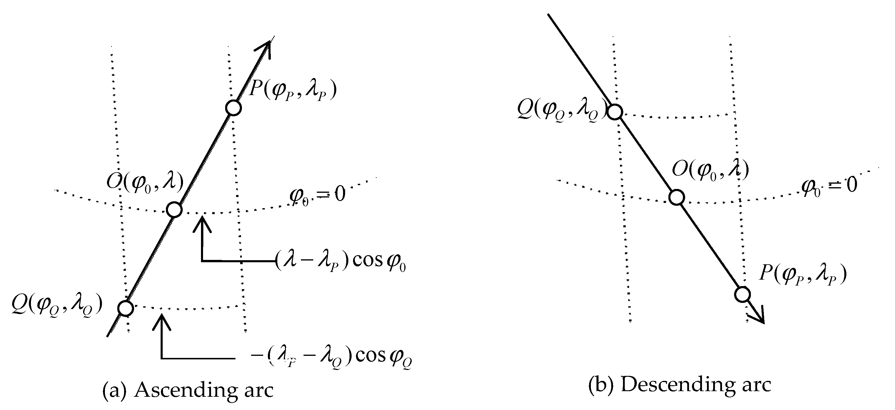
2.2. Interpolation Methods of Ground Track
2.3. The Orbit Prediction Strategy
3. Tests and Results
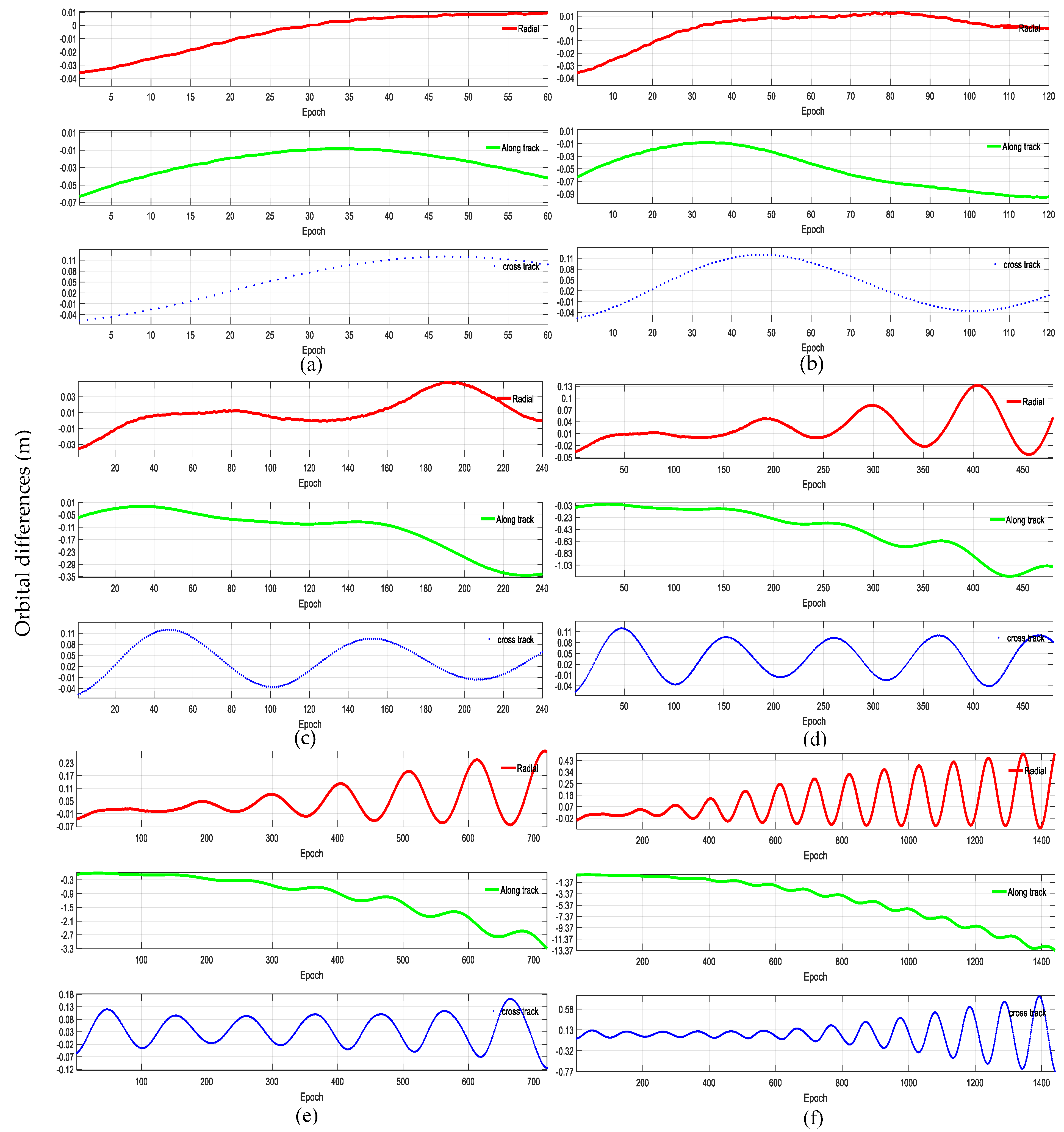
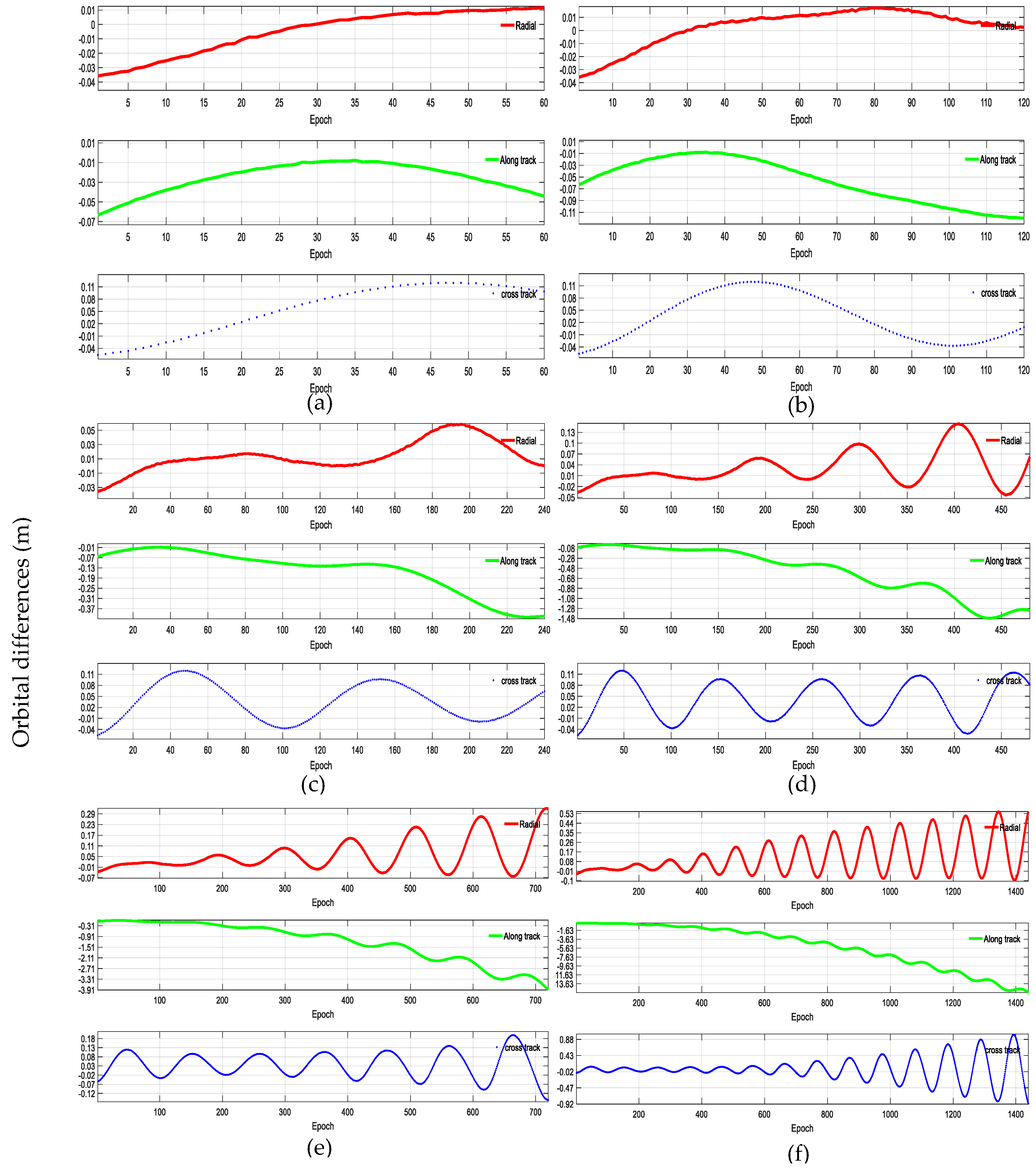
3.1. Predicted Orbit and SSALTO Orbit Comparison within Short-Term and Long-Term Arc Periods
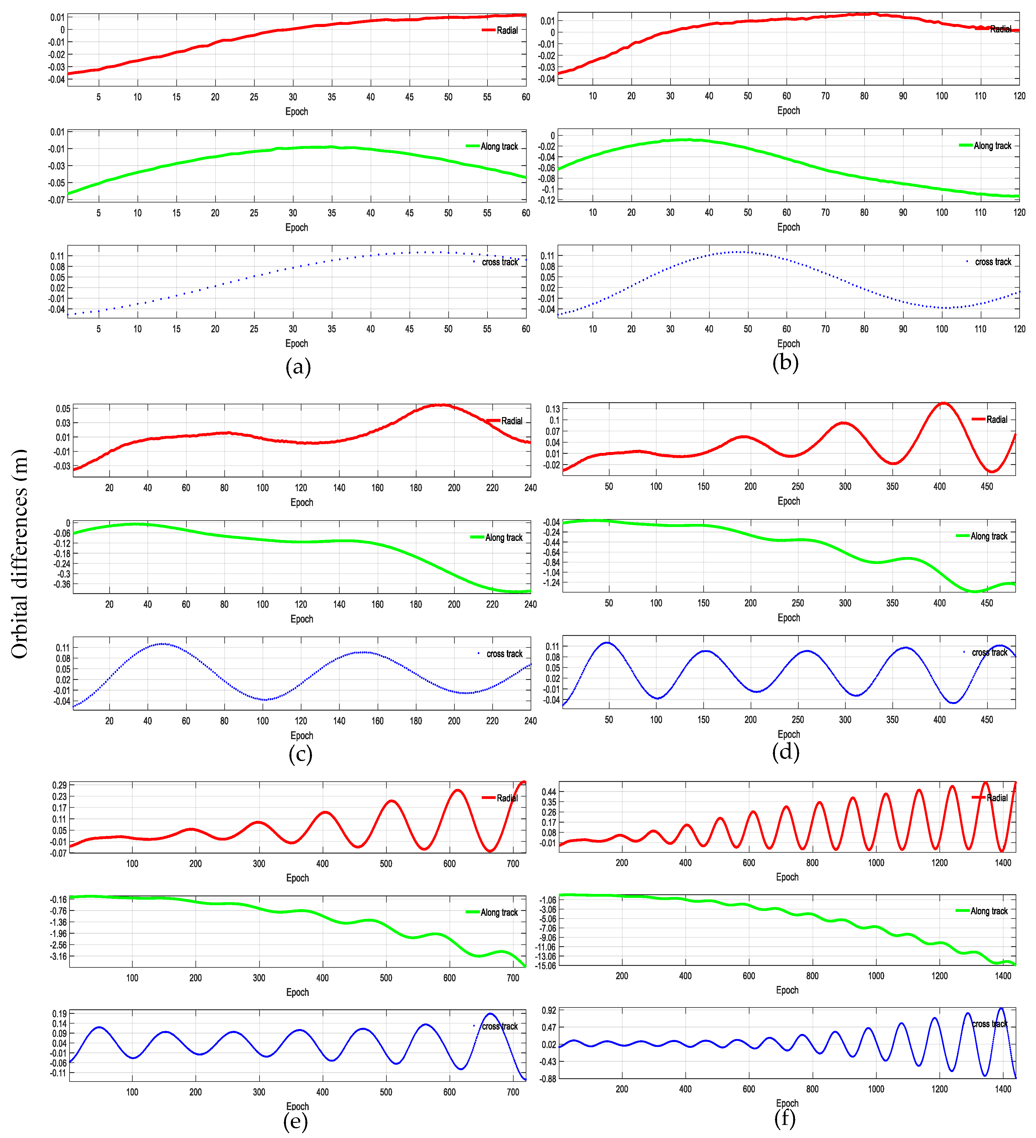
3.1.1. Orbital Comparison within Short-Term Arc Period
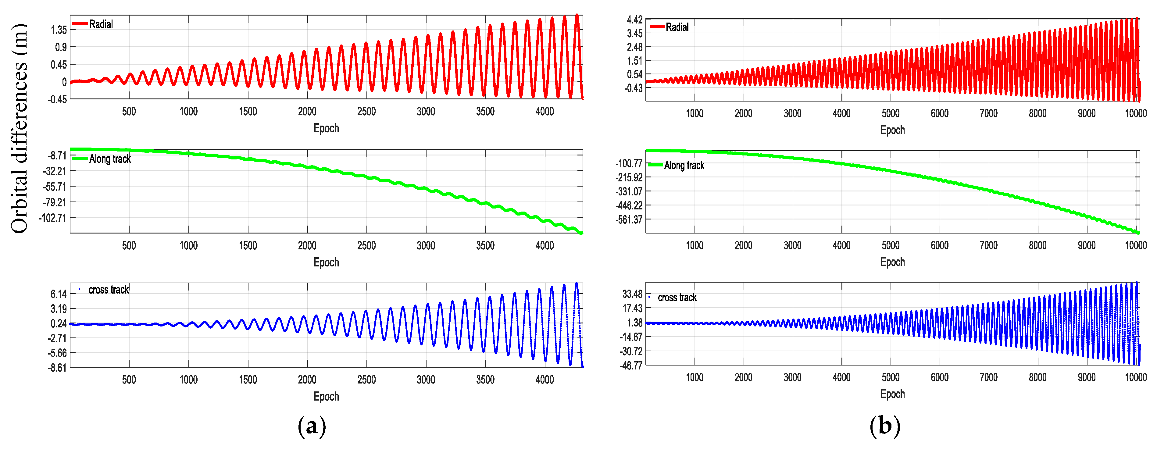
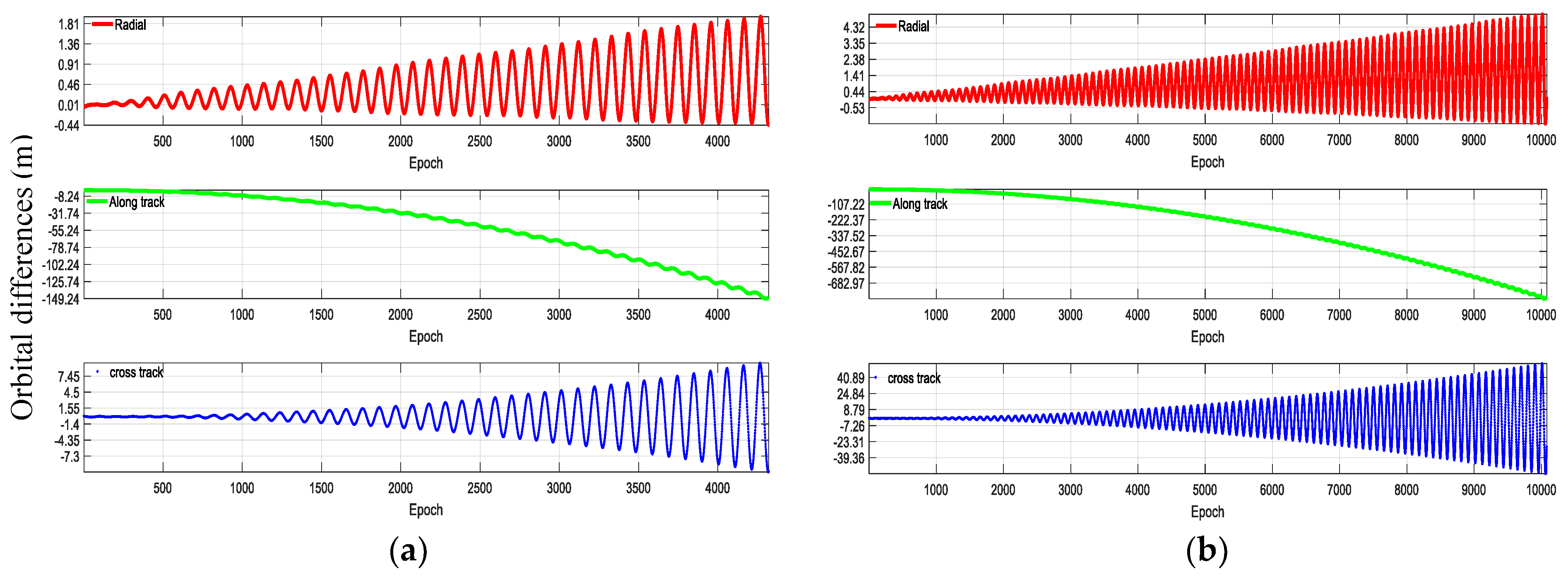
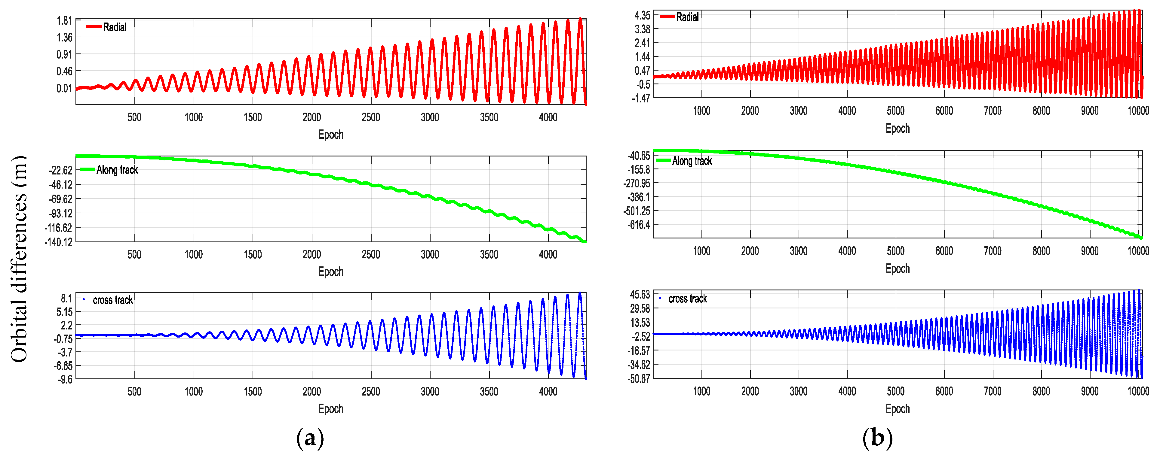
3.1.2. Orbital Comparison within a Long-Term Arc Period
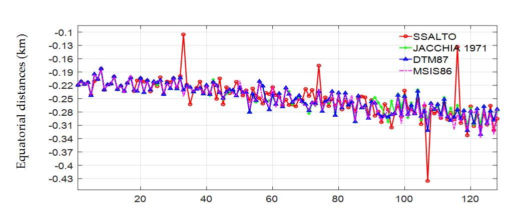
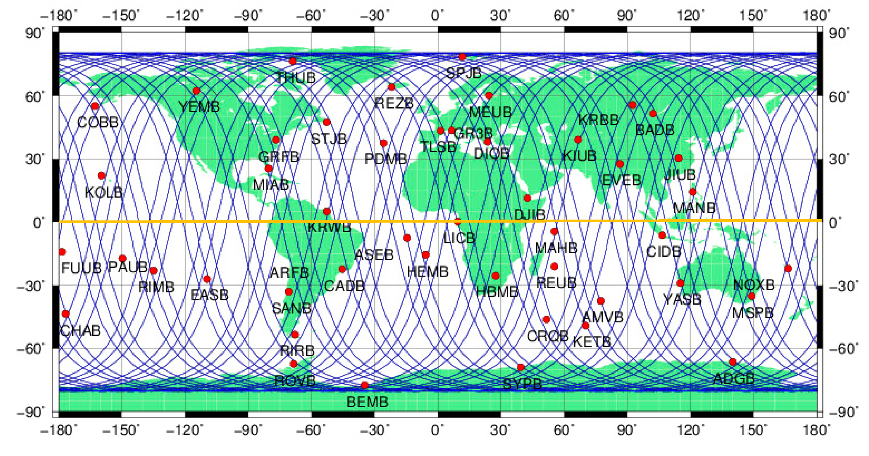
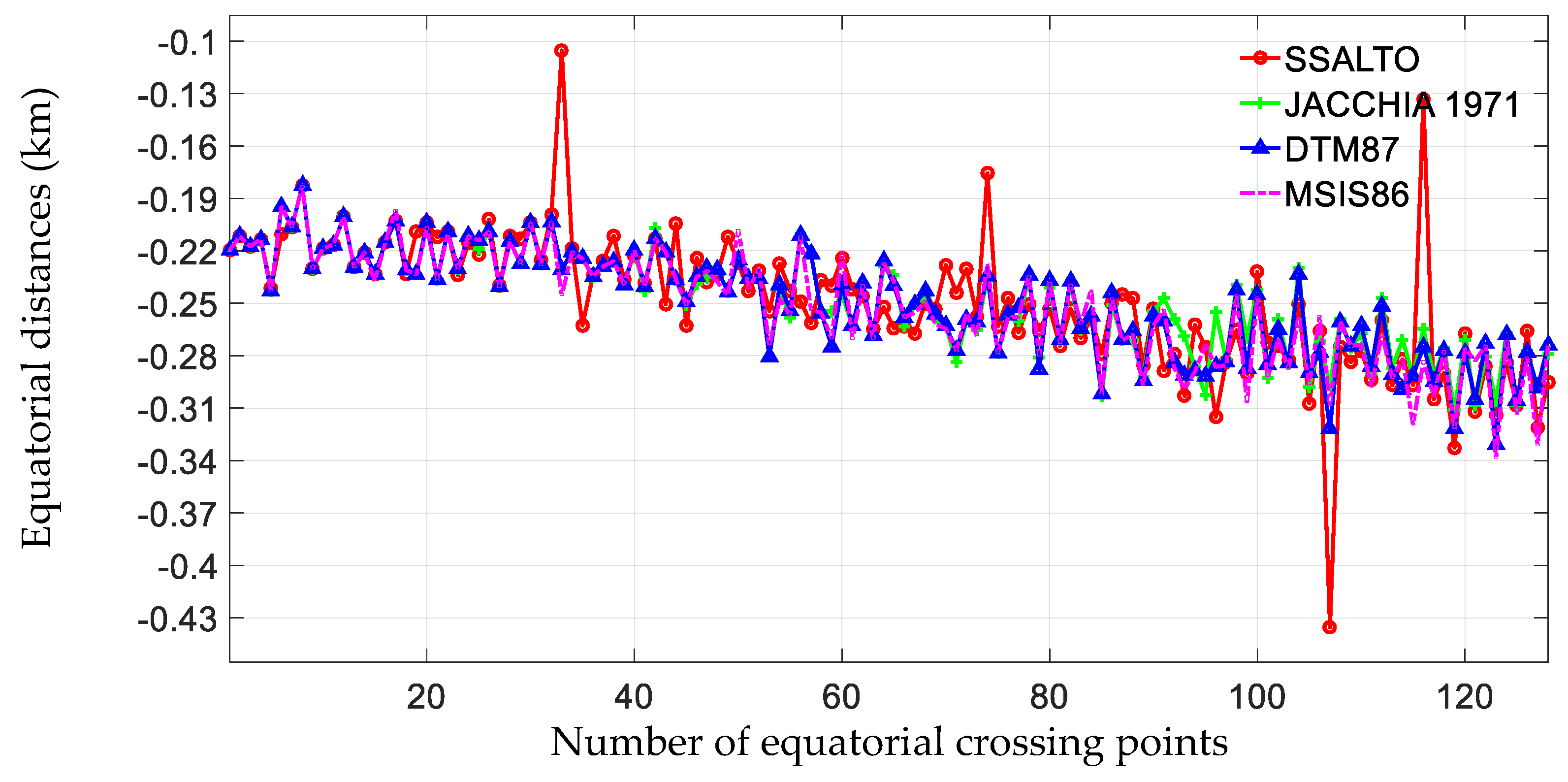
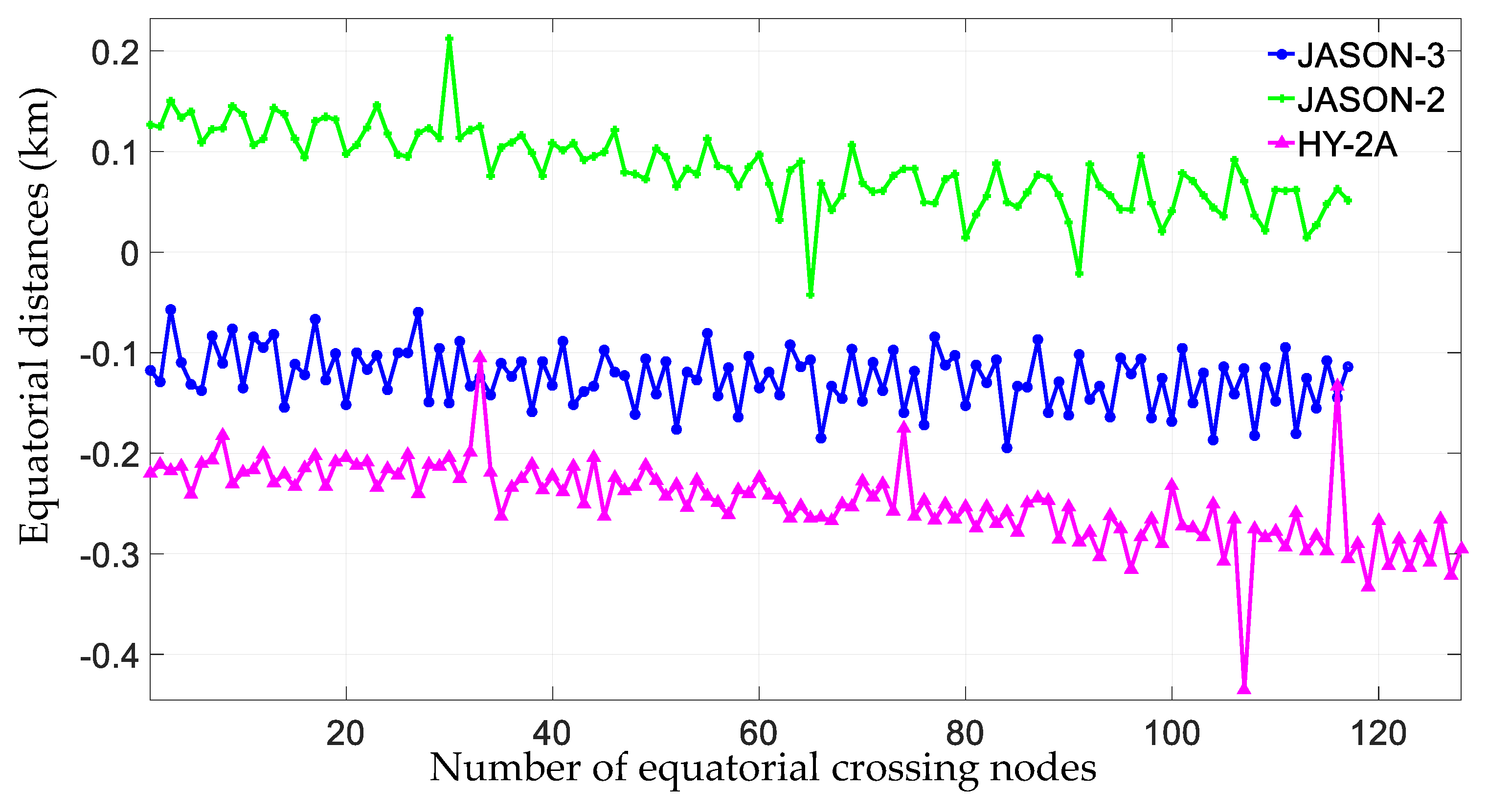
3.2. Analysis of Repeated Ground Track
4. Discussion
5. Conclusions
Author Contributions
Acknowledgments
Conflicts of Interest
References
- Meng, X.Q. Research and Application of Satellite Orbit Prediction Method Based on Osculating Kepler Element. Master’s Thesis, University of Chinese Academy of Sciences, Beijing, China, 2017. (In Chinese). [Google Scholar]
- Circi, C.; Ortore, E.; Bunkheila, F. Satellite constellations in sliding ground track orbits. Aerosp. Sci. Technol. 2014, 39, 395–402. [Google Scholar] [CrossRef]
- Wu, X.Y. Research and Application on Remote Sensing Satellite High Precision to Cover the Distributed Algorithm Based on the Geometric Topology. Master’s Thesis, Henan University, Zhengzhou, China, 2016. (In Chinese). [Google Scholar]
- Mur, T.J.M.; Springer, T.; Bar-Sever, Y. Orbit predictions and rapid products. In Proceedings of the 1998 Analysis Centre Workshop of the International GPS Service for Geodynamics (IGS), Darmstadt, Germany, 9–11 February 1998. [Google Scholar]
- Romay, M.M.; Lainez, M.D. Generation of precise long-term orbit and clock prediction products for A-GNSS. In Proceedings of the International Technical Meeting of the Satellite Division of the Institute of Navigation, Nashville, TN, USA, 17–21 September 2012. [Google Scholar]
- Polle, B.; Sidorov, D.; Marie, S.; Dach, R.; Gonzalez, F. Orbit/SRP modelling for long term prediction. In Proceedings of the IGS Workshop 2017, Paris, France, 3–7 July 2017. [Google Scholar]
- Wang, Y.; Zhong, S.; Wang, H.; Ou, J. Precision analysis of LEO satellite orbit prediction. Acta Geod. Cartogr. Sin. 2016, 45, 1035–1041. (In Chinese) [Google Scholar]
- Zhu, Y.H.; Chao, X.; Cai, C.L. Method and analysis of medium and long term satellite orbit prediction based on satellite broadcast ephemeris parameters. Int. J. Future Gener. Commun. Netw. 2015, 8, 187–196. [Google Scholar] [CrossRef]
- Tang, J.; Liu, L.; Cheng, H.; Hu, S.; Duan, J. Long-term orbit prediction for TianGong-1 spacecraft using the mean atmosphere model. Adv. Space Res. 2015, 55, 1432–1444. [Google Scholar] [CrossRef]
- Hartikainen, J.; Seppanen, M.; Sarkka, S. State-space inference for non-linear latent force models with application to satellite orbit prediction. In Proceedings of the 29th International Conference on Machine Learning, Edinburgh, Scotland, UK, 26 June–1 July 2012; pp. 1206–1215. [Google Scholar]
- Jacchia, L.G. Revised Static Models of the Thermosphere and Exosphere with Empirical Temperature Profiles; Special Report in Smithsonian Astrophysical Observatory; SAO: Cambridge, MA, USA, 1971. [Google Scholar]
- Hedin, A.E. MSIS-86 thermospheric model. J. Geophys. Res. 1987, 92, 4649–4662. [Google Scholar] [CrossRef]
- Gaposchkin, E.M.; Coster, A.J. Analysis of satellite drag. Lincoln Lab. J. 1988, 1, 203–224. [Google Scholar]
- Martin, T. MicroCosm System Description; Van Martin Systems Inc.: Green Bay, WI, USA, 2011. [Google Scholar]
- Montenbruck, O.; Gill, E. Satellite Orbits: Models Methods Applications, 2nd ed.; Springer: Heidelberg, Germany, 2001; pp. 91–102. ISBN 3-540-67280-X. [Google Scholar]
- Vallado, D.A.; Finkleman, D. A critical assessment of satellite drag and atmospheric density modeling. Acta Astronaut. 2014, 95, 141–165. [Google Scholar] [CrossRef]
- Fattig, E.; McLaughlin, C.; Lechtenberg, T. Comparison of Density Estimation for CHAMP and GRACE Satellites. In Proceedings of the AIAA/AAS Astrodynamics Specialist Conference, Toronto, ON, Canada, 2–5 August 2010. [Google Scholar]
- Thaheer, A.S.M.; Ismail, N.A. Orbit Design and Lifetime Analysis of MYSat: A 1U CubeSat for Electron-density Measurement. In Proceedings of the 4th NatGrad Conference, Uniten, Malaysia, 26–27 April 2017. [Google Scholar]
- Berger, C.; Biancale, R.; Ill, M.; Barlier, F. Improvement of the empirical thermospheric model DTM: DTM-94—A comparative review of various temporal variations and prospects in space geodesy applications. J. Geodesy 1998, 72, 161–178. [Google Scholar] [CrossRef]
- Knudsen, P.; Brovelli, M. Collinear and cross-over adjustment of Geosat ERM and Seasat altimeter data in the Mediterranean Sea. Surv. Geophys. 1993, 14, 449–459. [Google Scholar] [CrossRef]
- Scharroo, R.; Visser, P. Precise orbit determination and gravity field improvement for the ERS satellites. J. Geophys. Res. Oceans 1998, 103, 8113–8127. [Google Scholar] [CrossRef] [Green Version]
- Montenbruck, O.; Gill, E. Satellite Tracking and Observation Models, Satellite Orbits, 1st ed.; Springer: Heidelberg, Germany, 2000; pp. 87–98. ISBN 978-3-642-58351-3. [Google Scholar]
- Balmino, G.; Barriot, J.P. Numerical integration techniques revisited. Manuscr. Geod. 1990, 15, 1–10. [Google Scholar]
- Pavlis, N.K.; Holmes, S.A.; Kenyon, S.C.; Factor, J.K. The development and evaluation of the Earth Gravitational Model 2008 (EGM2008). J. Geophys. Res. Solid Earth 2012, 117, 1–38. [Google Scholar] [CrossRef]
- Standish, E.M. JPL Planetary and Lunar Ephemerides, DE405/LE405; Jet Propulsion Laboratory, InterOffice Memorandum (IOM): Pasadena, CA, USA, 1998; pp. 1–18. [Google Scholar]
- Petit, G.; Luzum, B. IERS Conventions (2010); Bureau International des Poids et Mesures: Sèvres, France, 2010. [Google Scholar]
- Lyard, F.; Lefevre, F.; Letellier, T.; Francis, O. Modeling the global ocean tides: Modern insights from FES2004. Ocean Dyn. 2006, 56, 394–415. [Google Scholar] [CrossRef]
- McCarthy, D.D.; Petit, G. Equations of Motion for an Artificial Earth Satellite; IERS Technical Note 32; IERS Conventions: Paris, France, 2003. [Google Scholar]
- Rim, H.J. TOPEX Orbit Determination Using GPS Tracking System. Ph.D. Thesis, University of Texas at Austin, Austin, TX, USA, 1992. [Google Scholar]
- Knocke, P.C.; Ries, J.C.; Tapley, B.D. Earth radiation pressure effects on satellites. In Proceedings of the AIAA/AAS Astrodynamics Conference, Guidance, Navigation, and Control and Co-Located Conferences, Reston, VA, USA, 15–17 August 1998; pp. 577–587. [Google Scholar]
- Goad, C.C.; Goodman, L. A modified Hopfield tropospheric refraction correction model. In Proceedings of the American Geophysical Union Annual Fall Meeting, San Francisco, CA, USA, 12–17 December 1974. [Google Scholar]
- Gao, F.; Peng, B.; Zhang, Y.; Evariste, N.H.; Liu, J.; Wang, X.; Zhong, M.; Lin, M.; Wang, N.; Chen, R.; et al. Analysis of HY2A precise orbit determination using DORIS. Adv. Space Res. 2015, 55, 1394–1404. [Google Scholar] [CrossRef]


| Items | Description |
|---|---|
| Coordinates of DORIS beacon stations | http://www.ipgp.fr/~willis/DPOD2008/ |
| Earth gravity model | EGM2008 [24], 80 × 80 |
| N-body | JPL DE403 [25] |
| Solid Earth tides | IERS2010 [26] |
| Ocean tides and ocean tide loading | FES2004 [27] |
| Relativistic effect | IERS2003 [28] |
| Solar radiation pressure | Box-Wing [29] |
| Earth albedo radiation | Knocke–Ries–Tapley [30] |
| Tropospheric model | Hopfied [31] |
| Atmospheric drag | MSIS86 [12], Jacchia 1971 [11], DTM87 [13] |
| Surface (m2) | Normal in Satellite Reference Frame | Optical Properties | Infrared Properties | ||||
|---|---|---|---|---|---|---|---|
| X | Y | Z | Diffuse | Emissivity | Diffuse | Emissivity | |
| 2.50 | 1 | 0.54 | 0.46 | 0.31 | 0.69 | ||
| 2.92 | −1 | 0.54 | 0.46 | 0.31 | 0.69 | ||
| 5.85 | 1 | 0.54 | 0.46 | 0.31 | 0.69 | ||
| 6.74 | −1 | 0.54 | 0.46 | 0.31 | 0.69 | ||
| 4.93 | 1 | 0.54 | 0.46 | 0.31 | 0.69 | ||
| 4.60 | −1 | 0.54 | 0.46 | 0.31 | 0.69 | ||
| 9.06 | −1 | 0.36 | 0.64 | 0.16 | 0.84 | ||
| 9.06 | 1 | 0.06 | 0.94 | 0.06 | 0.94 | ||
| 0.71 | 1 | 0.85 | 0.15 | 0.21 | 0.79 | ||
| 0.60 | 1 | 0.85 | 0.15 | 0.21 | 0.79 | ||
| 0.89 | 1 | 0.73 | 0.27 | 0.13 | 0.87 | ||
| 1.50 | 1 | 0.85 | 0.15 | 0.21 | 0.79 | ||
| 1.80 | 1 | 0.85 | 0.15 | 0.21 | 0.79 | ||
| Radial | Along Track | Cross Track | 3-D | ||||
|---|---|---|---|---|---|---|---|
| (Standard Deviation) STD | RMS | STD | RMS | STD | RMS | RMS | |
| 1 h | 0.015 | 0.016 | 0.015 | 0.029 | 0.061 | 0.082 | 0.089 |
| 2 h | 0.013 | 0.013 | 0.030 | 0.059 | 0.057 | 0.065 | 0.089 |
| 4 h | 0.018 | 0.021 | 0.103 | 0.160 | 0.048 | 0.059 | 0.172 |
| 8 h | 0.039 | 0.045 | 0.382 | 0.579 | 0.048 | 0.062 | 0.584 |
| 12 h | 0.077 | 0.091 | 0.921 | 1.363 | 0.058 | 0.068 | 1.367 |
| 24 h | 0.144 | 0.176 | 4.101 | 6.045 | 0.262 | 0.265 | 6.054 |
| Radial | Along Track | Cross Track | 3-D | ||||
|---|---|---|---|---|---|---|---|
| STD | RMS | STD | RMS | STD | RMS | RMS | |
| 1 h | 0.015 | 0.016 | 0.015 | 0.029 | 0.061 | 0.082 | 0.089 |
| 2 h | 0.014 | 0.014 | 0.038 | 0.068 | 0.057 | 0.065 | 0.095 |
| 4 h | 0.021 | 0.025 | 0.128 | 0.195 | 0.049 | 0.060 | 0.206 |
| 8 h | 0.044 | 0.053 | 0.467 | 0.707 | 0.051 | 0.065 | 0.712 |
| 12 h | 0.086 | 0.103 | 1.102 | 1.639 | 0.069 | 0.078 | 1.644 |
| 24 h | 0.160 | 0.200 | 4.783 | 7.084 | 0.314 | 0.316 | 7.094 |
| Radial | Along Track | Cross Track | 3-D | ||||
|---|---|---|---|---|---|---|---|
| STD | RMS | STD | RMS | STD | RMS | RMS | |
| 1 h | 0.015 | 0.016 | 0.015 | 0.029 | 0.061 | 0.082 | 0.089 |
| 2 h | 0.014 | 0.014 | 0.036 | 0.067 | 0.057 | 0.065 | 0.094 |
| 4 h | 0.020 | 0.024 | 0.124 | 0.191 | 0.049 | 0.060 | 0.201 |
| 8 h | 0.042 | 0.050 | 0.454 | 0.690 | 0.051 | 0.064 | 0.695 |
| 12 h | 0.082 | 0.099 | 1.056 | 1.578 | 0.067 | 0.076 | 1.583 |
| 24 h | 0.153 | 0.191 | 4.591 | 6.800 | 0.300 | 0.302 | 6.809 |
| Radial | Along Track | Cross Track | 3-D | ||||
|---|---|---|---|---|---|---|---|
| STD | RMS | STD | RMS | STD | RMS | RMS | |
| 3 days | 0.475 | 0.573 | 37.488 | 56.006 | 2.664 | 2.664 | 56.073 |
| 7 days | 1.210 | 1.421 | 201.783 | 303.025 | 14.812 | 14.812 | 303.39 |
| Radial | Along Track | Cross Track | 3-D | ||||
|---|---|---|---|---|---|---|---|
| STD | RMS | STD | RMS | STD | RMS | RMS | |
| 3 days | 0.532 | 0.653 | 44.304 | 66.073 | 3.171 | 3.171 | 66.152 |
| 7 days | 1.361 | 1.621 | 238.858 | 358.794 | 17.622 | 17.621 | 359.23 |
| Radial | Along Track | Cross Track | 3-D | ||||
|---|---|---|---|---|---|---|---|
| STD | RMS | STD | RMS | STD | RMS | RMS | |
| 3 days | 0.502 | 0.616 | 41.653 | 62.332 | 2.982 | 2.983 | 62.406 |
| 7 days | 1.272 | 1.506 | 219.122 | 330.629 | 16.202 | 16.202 | 331.029 |
| 3-Day Arc | 7-Day Arc | |||||
|---|---|---|---|---|---|---|
| SSALTO- Jacchia 1971 | SSALTO- MMIS86 | SSALTO- DTM87 | SSALTO- Jacchia 1971 | SSALTO- MSIS86 | SSALTO- DTM87 | |
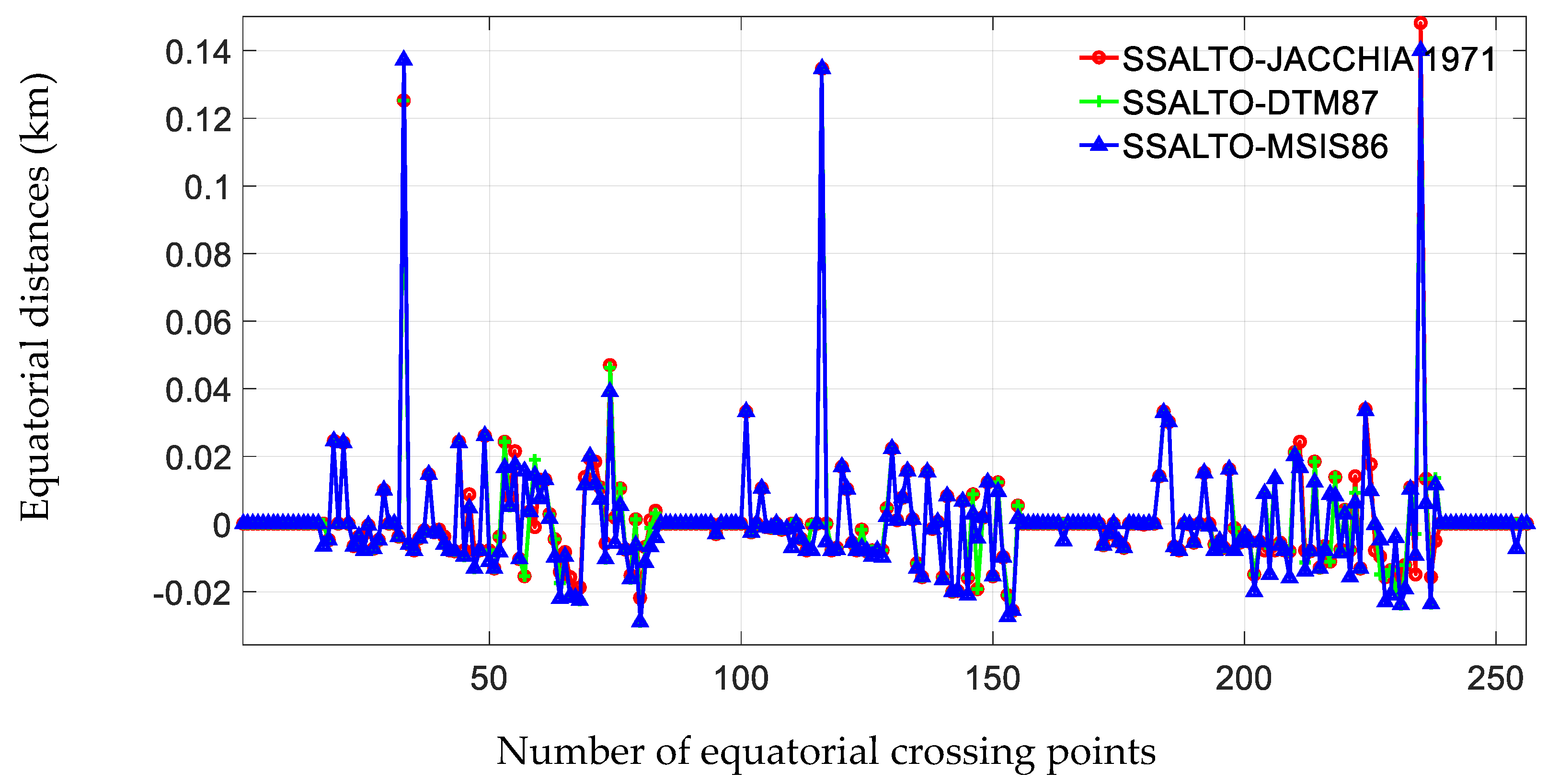
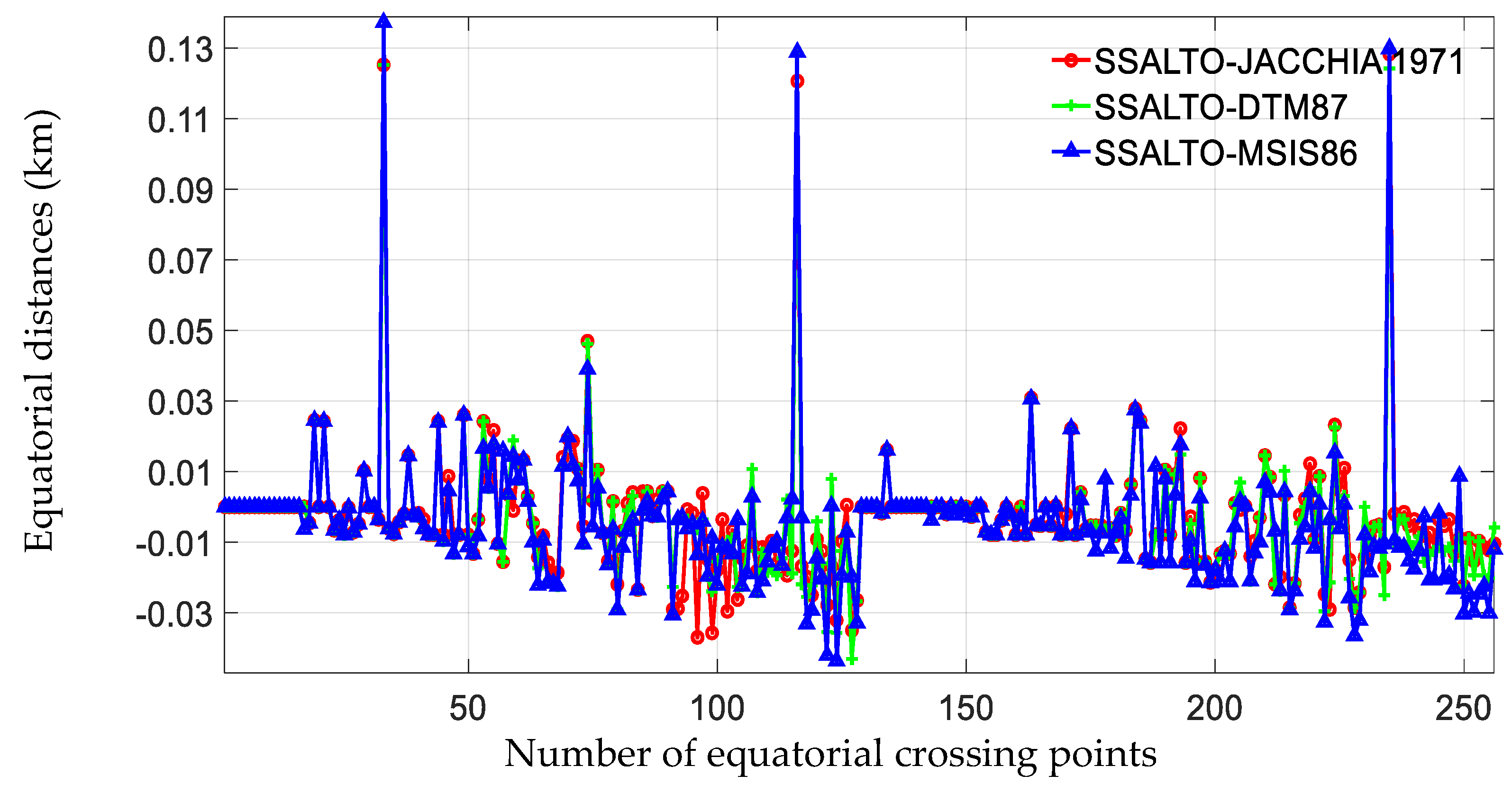
| MAX | 0.1380 | 0.1401 | 0.1381 | 0.1282 | 0.1372 | 0.1289 |
| MIN | −0.0257 | −0.029 | −0.0290 | −0.037 | −0.0437 | −0.043 |
| STD | 0.0171 | 0.0184 | 0.0180 | 0.0186 | 0.0196 | 0.0187 |
| RMS | 0.0171 | 0.0184 | 0.0180 | 0.0188 | 0.0200 | 0.0190 |
| 3-day Arc | 7-day Arc | ||||||
|---|---|---|---|---|---|---|---|
| SSALTO | Jacchia 1971 | MSIS86 | DTM87 | Jacchia 1971 | MSIS86 | DTM87 | |
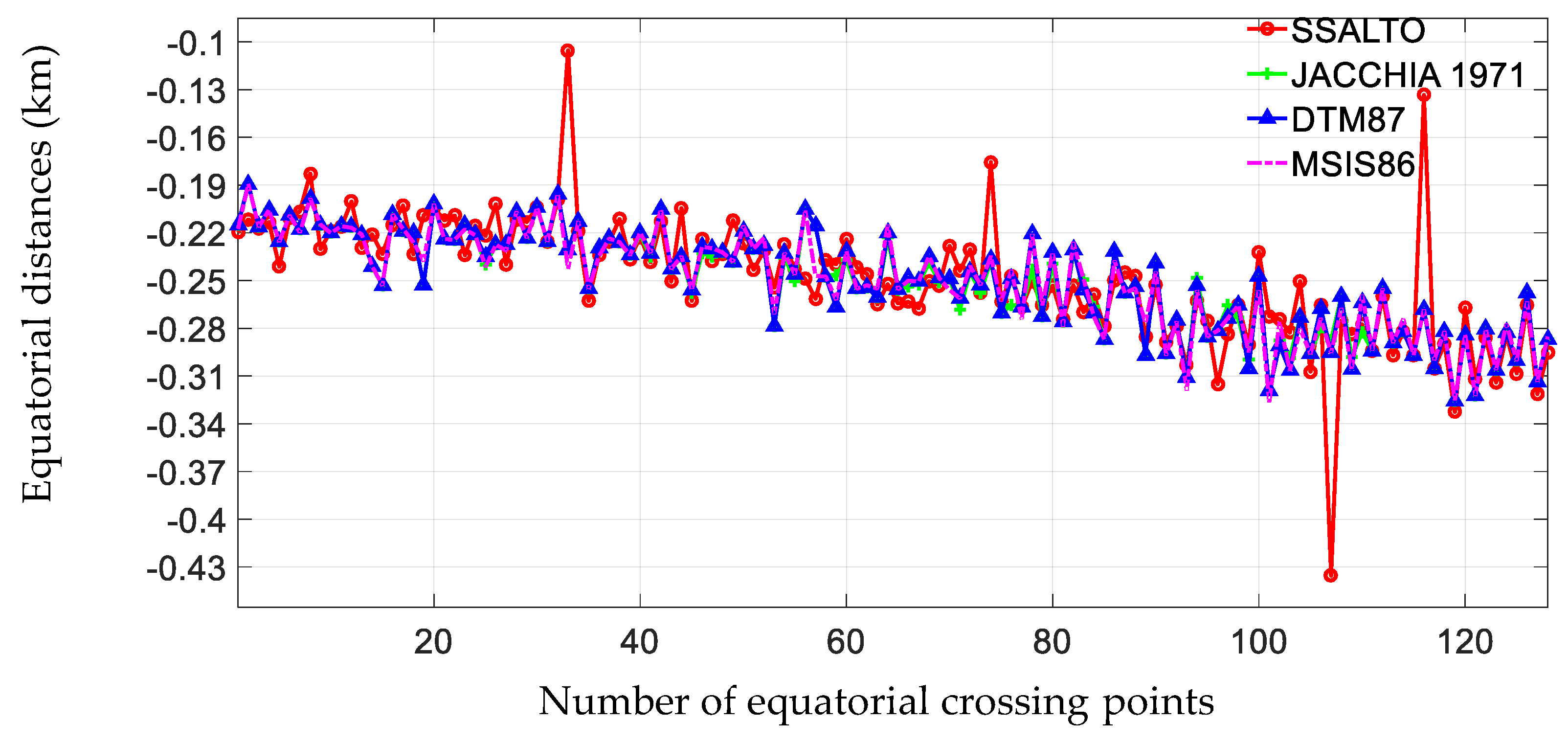
| MAX | −0.1053 | −0.1894 | −0.1894 | −0.1894 | −0.1827 | −0.1827 | −0.1827 |
| MIN | −0.4354 | −0.3251 | −0.3266 | −0.3256 | −0.3112 | −0.3389 | −0.3308 |
| STD | 0.0395 | 0.0311 | 0.0315 | 0.0320 | 0.0290 | 0.0322 | 0.0352 |
| RMS | 0.2515 | 0.2519 | 0.2521 | 0.2521 | 0.2505 | 0.2535 | 0.2526 |
| MAX | MIN | STD | RMS | |
|---|---|---|---|---|
| JASON-3 | −0.0570 | −0.1946 | 0.0281 | 0.1276 |
| JASON-2 | 0.2122 | −0.0426 | 0.0379 | 0.0915 |
| HY-2A | −0.1053 | −0.4354 | 0.0395 | 0.2515 |
© 2018 by the authors. Licensee MDPI, Basel, Switzerland. This article is an open access article distributed under the terms and conditions of the Creative Commons Attribution (CC BY) license (http://creativecommons.org/licenses/by/4.0/).
Share and Cite
Kong, Q.; Gao, F.; Guo, J.; Han, L.; Zhang, L.; Shen, Y. Analysis of Precise Orbit Predictions for a HY-2A Satellite with Three Atmospheric Density Models Based on Dynamic Method. Remote Sens. 2019, 11, 40. https://0-doi-org.brum.beds.ac.uk/10.3390/rs11010040
Kong Q, Gao F, Guo J, Han L, Zhang L, Shen Y. Analysis of Precise Orbit Predictions for a HY-2A Satellite with Three Atmospheric Density Models Based on Dynamic Method. Remote Sensing. 2019; 11(1):40. https://0-doi-org.brum.beds.ac.uk/10.3390/rs11010040
Chicago/Turabian StyleKong, Qiaoli, Fan Gao, Jinyun Guo, Litao Han, Linggang Zhang, and Yi Shen. 2019. "Analysis of Precise Orbit Predictions for a HY-2A Satellite with Three Atmospheric Density Models Based on Dynamic Method" Remote Sensing 11, no. 1: 40. https://0-doi-org.brum.beds.ac.uk/10.3390/rs11010040