Article

A Multi-Platform Hydrometeorological Analysis of the Flash Flood Event of 15 November 2017 in Attica, Greece

by
George Varlas
1,2,
Marios N. Anagnostou
3,4,5,
Christos Spyrou
1,
Anastasios Papadopoulos
2,*,
John Kalogiros
3,
Angeliki Mentzafou
2,
Silas Michaelides
6,
Evangelos Baltas
5,
Efthimios Karymbalis
1 and
Petros Katsafados
1
1
Department of Geography, Harokopio University of Athens, HUA, 17671 Athens, Greece
2
Institute of Marine Biological Resources and Inland Waters, Hellenic Centre for Marine Research, HCMR, 19013 Anavyssos, Greece
3
National Observatory of Athens, IERSD, 15236 Athens, Greece
4
Department of Environmental Sciences, Ionian University, 29100 Zakynthos, Greece
5
Department of Water Resources, School of Civil Engineering, NTUA, 10682 Athens, Greece
6
The Cyprus Institute, 20, Konstantinou Kavafi Str., Aglantzia, CY2121 Nicosia, Cyprus
*
Author to whom correspondence should be addressed.
Submission received: 13 November 2013 / Revised: 17 December 2018 / Accepted: 21 December 2018 / Published: 28 December 2018
(This article belongs to the Special Issue Remote Sensing of Precipitation)

Abstract

:
Urban areas often experience high precipitation rates and heights associated with flash flood events. Atmospheric and hydrological models in combination with remote-sensing and surface observations are used to analyze these phenomena. This study aims to conduct a hydrometeorological analysis of a flash flood event that took place in the sub-urban area of Mandra, western Attica, Greece, using remote-sensing observations and the Chemical Hydrological Atmospheric Ocean Wave System (CHAOS) modeling system that includes the Advanced Weather Research Forecasting (WRF-ARW) model and the hydrological model (WRF-Hydro). The flash flood was caused by a severe storm during the morning of 15 November 2017 around Mandra area resulting in extensive damages and 24 fatalities. The X-band dual-polarization (XPOL) weather radar of the National Observatory of Athens (NOA) observed precipitation rates reaching 140 mm/h in the core of the storm. CHAOS simulation unveils the persistent orographic convergence of humid southeasterly airflow over Pateras mountain as the dominant parameter for the evolution of the storm. WRF-Hydro simulated the flood using three different precipitation estimations as forcing data, obtained from the CHAOS simulation (CHAOS-hydro), the XPOL weather radar (XPOL-hydro) and the Global Precipitation Measurement (GMP)/Integrated Multi-satellitE Retrievals for GPM (IMERG) satellite dataset (GPM/IMERG-hydro). The findings indicate that GPM/IMERG-hydro underestimated the flood magnitude. On the other hand, XPOL-hydro simulation resulted to discharge about 115 m3/s and water level exceeding 3 m in Soures and Agia Aikaterini streams, which finally inundated. CHAOS-hydro estimated approximately the half water level and even lower discharge compared to XPOL-hydro simulation. Comparing site-detailed post-surveys of flood extent, XPOL-hydro is characterized by overestimation while CHAOS-hydro and GPM/IMERG-hydro present underestimation. However, CHAOS-hydro shows enough skill to simulate the flooded areas despite the forecast inaccuracies of numerical weather prediction. Overall, the simulation results demonstrate the potential benefit of using high-resolution observations from a X-band dual-polarization radar as an additional forcing component in model precipitation simulations.

Graphical Abstract

1. Introduction

Floods are considered one of the most frequent natural disasters, causing many fatalities and damages every year. In 2011, six out of 10 of the biggest natural disasters, on a global scale, were flash floods. The frequency of flooding events has increased in recent decades and a warmer climate is expected to aggravate their destruction potential and the effects on human life [1]. All climate model projections show that more frequent precipitation extremes are expected in warmer climates [2], particularly in the populated mid and high latitudes [3]. This is expected in turn to increase the flash flooding risk over urban areas with negative consequences.
Accurate estimation of precipitation has always been one of the most challenging physical based tasks due to its large spatial and temporal variability in regional and global scale [4]. Recent technological advances in ground- and space-borne remote-sensing precipitation measurements allows us to produce near-real-time rainfall estimates at high spatial and temporal resolutions, from hundreds of kilometers up to quasi-global coverage, making this data potentially useful for hydrological and other applications. Ground-based remote-sensing observations are usually performed by either one or a network of meteorological radars, which provide real-time high spatiotemporal-resolution precipitation monitoring. Nevertheless, the weather radars are also suffering from limitations and uncertainties, including limited coverage, variable accuracy, and limited utility in complex terrains [5,6]. Past studies [7,8,9,10,11,12] have shown that locally deployed X-band dual-polarization (XPOL) radar systems can contribute to higher-resolution rain rate estimations and improved rainfall quantification accuracies than the lower frequency (C-band and S-band) long-range operational radar systems. These short-range radar systems could potentially be used to fill in coverage gaps of operational weather radar networks, which is essential for early warning of precipitation driven hydrological hazards (flash floods, landslides, debris flows, etc.) in urban and small mountainous basins [13,14,15].
Technological advances over the past two decades on satellite precipitation products have been developed and extensively used for large-scale hydrological and precipitation studies [16,17,18]. In the past 20 years, two international precipitation missions, the Tropical Rainfall Measuring Mission (TRMM), which launched in 1997 and lasted through 2015, and its successor, the Global Precipitation Measurement (GPM) mission, Core Observatory (CO) satellite, launched in 2014, contributed to provide high-resolution precipitation radar (PR) measurements. The GPM mission initiated by the National Aeronautics and Space Administration (NASA) and the Japan Aerospace Exploration Agency (JAXA) was launched on 27 February 2014 to globally observe rain and snow with improved accuracy [19]. Subsequent to the GPM Core Observatory launch, an advanced high-resolution multi-satellite-based precipitation product that combines the advantages of PERSIANN-CCS (Precipitation Estimation from Remotely Sensed Information using Artificial Neural Networks-Cloud Classification System), CMORPH (Climate Prediction Center MORPHing technique), and TMPA (TRMM Multisatellite Precipitation Analysis) was incrementally released since late 2014, i.e., the Integrated Multi-satellitE Retrievals for GPM (IMERG). Although the accuracy of satellite precipitation products has improved over the past few decades, they always suffer from significant errors associated with indirect measurements of ground precipitation [6]. All these methods cannot provide ground precipitation directly but rely on monitoring or modeling the precipitation-related variables to estimate precipitation indirectly.
Flash floods are frequent over several parts of the Mediterranean region due to the local climate, which is prone to intense storms [20]. The Mediterranean basin is a transitional zone between the cold and wet climates of northern Europe and the hot and dry climates of low latitudes (North Africa). It is also characterized by high diversity in local climatic conditions [21]. Therefore, the types of precipitation that can generate flooding events vary along its coasts [20]. In general, convective thunderstorms and showers, which usually occur during late spring, summer and early autumn, are the main reason of flash flooding episodes [22]. In addition, the morphology of the drainage basins, the geographical characteristics of stream networks, and various anthropogenic interventions modify the response and the physical properties of the catchments [23]. Thus, these factors affect water cycle even exacerbating flash floods and their negative effects.
Greece experiences a variety of catastrophic weather events that are frequently followed by severe consequences on social and economic activity. Flash floods have caused tremendous loss of life and property over the past decades [24]. In Greece, they are primarily connected with strong convective storms developed during the warm season, especially over continental areas. These are mesoscale weather phenomena characterized by small spatial coverage (100 km2) and small-time scales, usually 1–2 h [25]. The potential of these storms to become hazardous for human life and infrastructure depends on whether the convection organizes into mesoscale convective systems which are characterized by spatial coverage of about 9000 km2 and time scales of about 5–8 h over Europe and the Mediterranean [26]. Sometimes, they are upgraded into long-lived mesoscale convective cells (supercells) with spatial coverage even exceeding 10,000 km2 and time scale reaching 2–3 days [27]. In any case, they distribute large amounts of water in a limited area very fast. In some cases, the response of watersheds to this type of rainfall events and their runoff rates are not fast enough, leading to flooding events [20]. The negative effects of these phenomena are aggravated in built riverside areas as prevention is a parameter usually ignored during urban planning [28].
A significant part of the drainage network of Greece consists of mountain torrents and small- to medium-size drainage basins with a limited amount of discharge capabilities for most of the year [29]. Even worse, several parts of the network are diminished, turned into streets or built upon, thus cutting off critical river cross sections [30]. The combination of highly intense convective storms and bad urban planning has led to a series of severe flash flood occurrences in Greece over the past years. In November 1993, several areas of southern Attica (mainly Glyfada and Voula) experienced severe flooding phenomena due to a sudden thunderstorm [31]. The flood caused serious property damage along with the destruction of public infrastructure (roads, bridges etc). Most of the damage was attributed to urbanization and road construction that had not considered the specific conditions around the area. On October 1994 and July 1995, two extreme rainfall events caused extensive flooding, damage to streets, houses and commercial areas, and overflow of water courses in a big part of Athens [32]. On 11 and 12 January 1997 a severe flood event caused loss of life and damage to houses, cultivation and constructions in the broader area of the city of Corinth due to an extreme rainfall and the human interference in the geomorphological characteristics of the local drainage network [33]. Mazi and Koussis [34] studied the overflowing of the Kifissos River in Athens due to a storm on the 8 July 2002, which was attributed to the hydraulic works underway in the lower part of the river at that time. More recently on 22 October 2015, Athens’s suburban areas were affected by a severe storm system, due to the passage of a barometric low associated with a cold front. The rainstorm caused extended flash flood incidents, mainly in the northern part of Athens, and led to the death of four people [35]. Summarizing, Diakakis et al. [29] performed a statistical analysis of available data and showed 686 fatalities due to a total of 545 flood events during the period 1880–2010 in Greece. In general, one of the most important factors for flash floods in Greece is the outbreak of intense rainfalls during the autumn and summer periods [24]. Geomorphology, soil characteristics (such as soil moisture), land use and human interference are also important factors.
Many studies present the efforts to simulate flash flooding events using numerical models, applying a multitude of systems like the hydrological model WRF-Hydro [36], DRiFt (Discharge River Forecast) [37], and CREST (Coupled Routing and Excess Storage) [38], for the hydrological part, and AROME (Applications of Research to Operations at Mesoscale model) [39], WRF (Weather Research and Forecasting model) [40,41], and others for the atmospheric component. The main aim of these models is the successful prediction of high-intensity rainfall often associated with convection and the simulation of channel- and surface-water runoff [22,42,43,44]. There are studies which rely on the combination of rain gauges and meteorological radar data [22,45,46]. Other studies use WRF model results, data assimilation techniques and satellite data to make forcing data for hydrological models like WRF-Hydro [43]. In general, a successful numerical simulation of a flash flood event requires the combination of an accurate atmospheric model, a suitable hydrological model and rainfall data of adequate spatial and temporal resolution [46].
The main aim of this study is to present a hydrometeorological analysis of an extreme flash flood event took place in the suburban area of Mandra, western Attica, Greece, using an integrated remote-sensing and observation-modeling system. This destructive flash flooding event occurred on 15 November 2017 causing 24 fatalities and extensive damage to property and infrastructure. The atmospheric conditions and the hydrological response of the drainage basin during the flood were simulated by the state-of-the-art modeling system CHAOS (Chemical Hydrological Atmospheric Ocean wave System [47,48], including the WRF-Hydro hydrological model [36]). To this end, three sensitivity tests using WRF-Hydro were performed in order to assess its hydrological response to different precipitation forcings. The first precipitation dataset was based on the results of the atmospheric component of CHAOS, the second on X-band dual-polarization experimental ground radar estimations and the third on GMP/IMERG satellite estimations. Post-survey and remote sensing maps were used to compare the extension of the flood [49,50,51]. The rest of the manuscript is organized as follows:
In Section 2, the geographical characteristics of study area and the methodology of remote sensing estimations are presented. Moreover, the set-up of CHAOS modeling system and the design of three different WRF-Hydro simulations are described. In Section 3, the meteorological conditions before and during the flood are analyzed through surface and upper air analysis charts. Section 4 presents the results of the three simulations focusing on the role of spatiotemporal characteristics of precipitation data on the hydrological characteristics of the flood. An evaluation of results using post-survey and satellite remote sensing maps is also presented. In Section 5, the main conclusions of this study are presented.

2. Materials and Methods
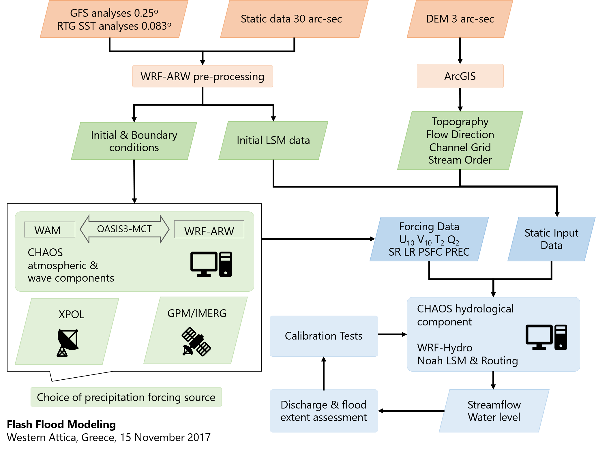
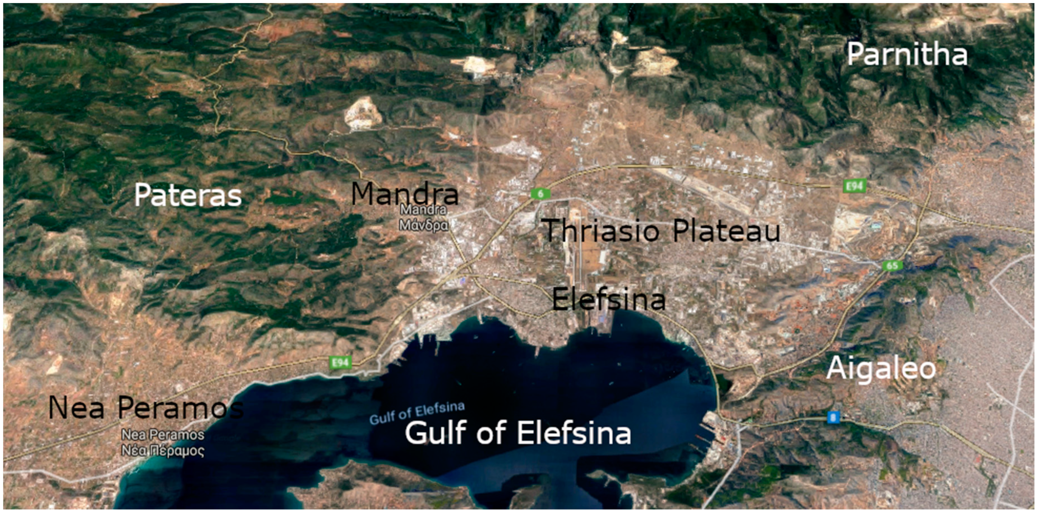
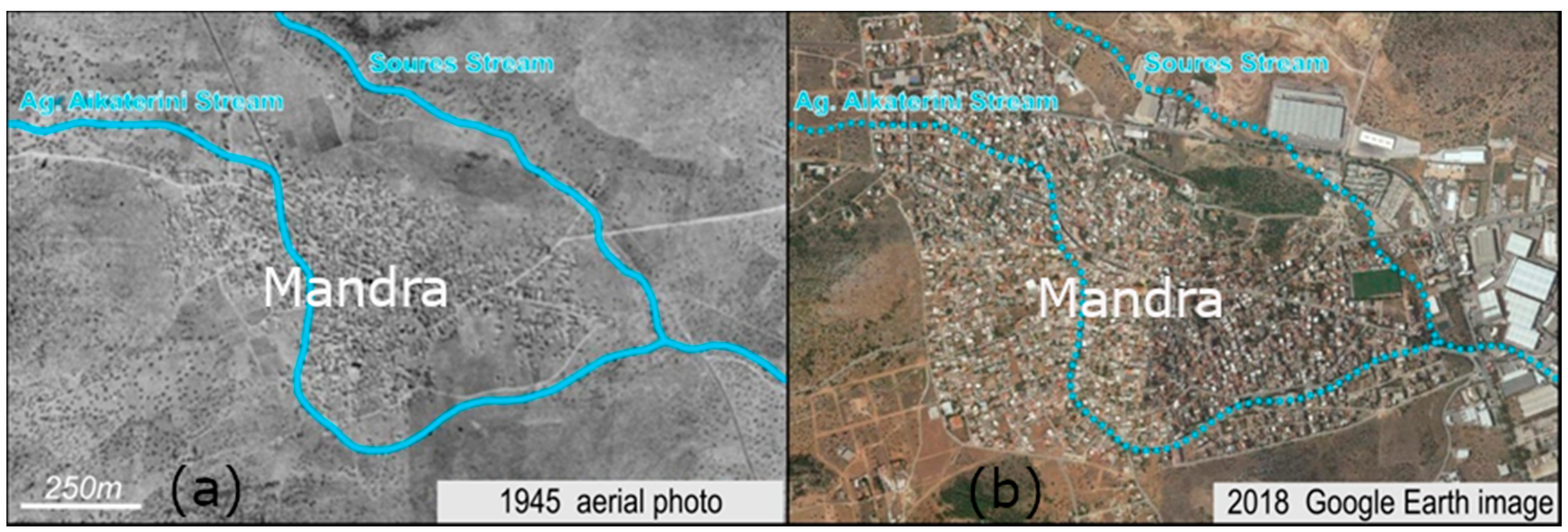
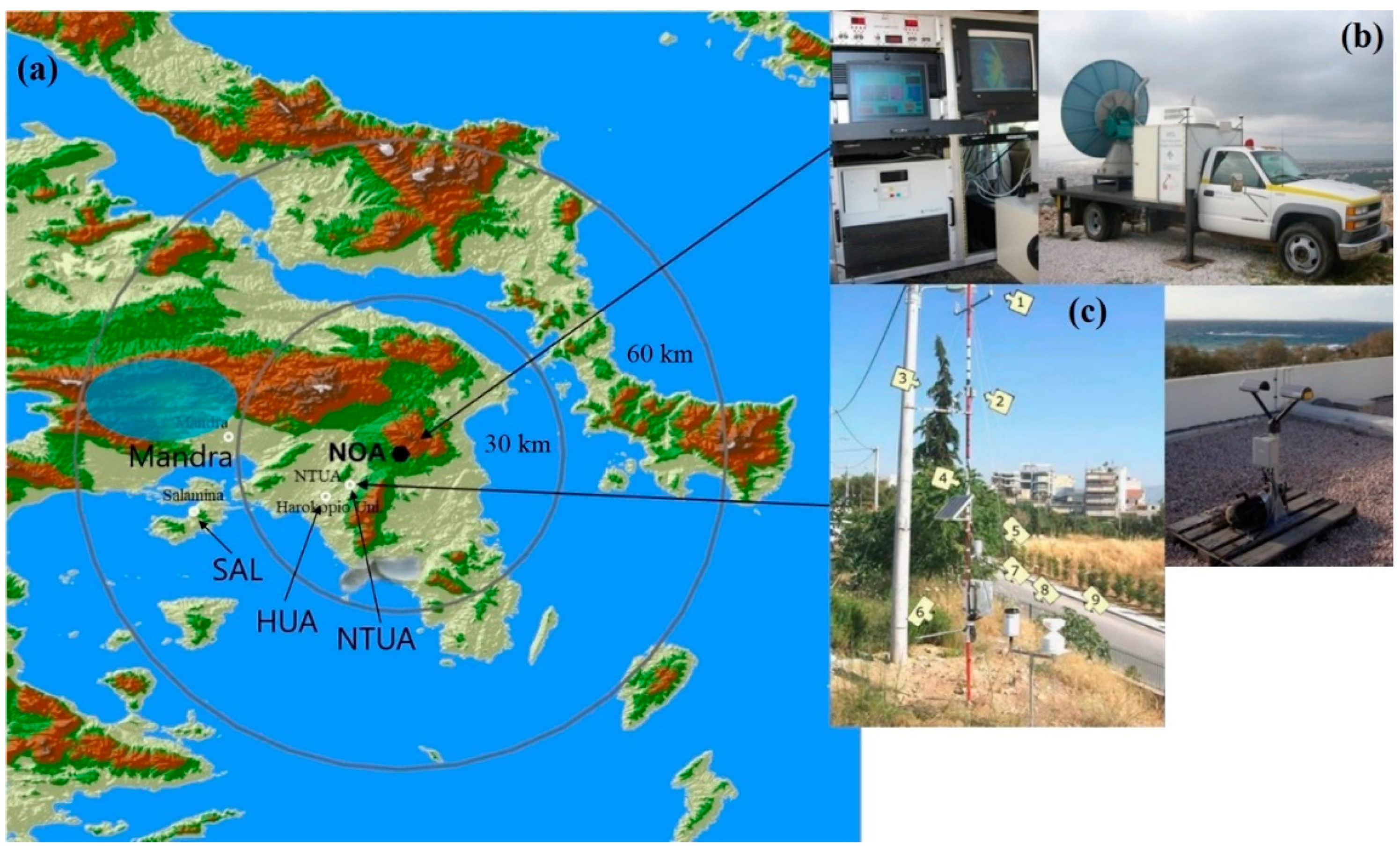
2.1. Study Area

Attica is an administrative region in Greece, situated at the southeasternmost point of central Greece. The whole region covers 3808 km2 and it is currently the most populated region of Greece, reaching 3.8 million inhabitants in 2011, with most of the population living in Athens. Attica experiences a typical Mediterranean climate with the mean annual precipitation ranging between 350 and 390 mm in the southwestern low-lying coastal region and 500 mm in the northeastern mountainous region [52]. Precipitation is distributed relatively unevenly with about 75% of it occurring between the months of October and March.
Western Attica hosts one of the largest industrial units in Greece including refineries, metallurgical industries, factories, shipyards as well as the waste landfill of all Attica prefecture. This industrial zone is included in Thriasio Plateau area covering a total range of 812.95 km2. The area is bounded by Pateras mountain (1016 m) from the west, Parnitha mountain (1413 m) from the north and Aigaleo mountain (468 m) from the east (Figure 1). The intense presence of heavy industry, urbanization and other land changes have worsened environmental pressures increasing the risk for flooding episodes. The residential and industrial development was lacking any appropriate plan regarding the infrastructure network for flood protection and drainage rainwater collection [53].
More specifically, the town of Mandra (Figure 1) is among the most damaged areas by the devastating November 2017 flood event. Mandra is a small industrial town, with a population of about 13,000 people, located 40 km west of Athens, which has significantly grown during recent decades. In term of lithology, the catchments consist exclusively of highly permeable geological formations (limestone and dolomites of Middle-Upper Triassic to Upper Cretaceous age which belong to the Subpelagonic geotectonic zone) [54] and streams of the drainage networks that are developed from alluvial deposits (mainly sands, silt and clays, gravels and pebbles). The town of Mandra is located at the apex of an alluvial fan formed by the two streams at the western part of the Thriassio plain. As depicted in Figure 2, the two main small ephemeral streams of the town are Soures and Agia Aikaterini which drain an area of 23.0 and 22.0 km2 respectively. These two streams meet at the southeastern edge of the town to form a river that discharges into the Gulf of Elefsina. Their drainage basins are elongated along an almost northwestern-southeastern trending axis and reach the elevation of 659 m and 800 m, respectively, at their western ends. Intensive construction activities in the greater area during the last decades resulted in significant morphological changes of the streams’ channels with most important the significant decrease of their available cross-sectional areas while in certain areas the streams practically vanished.
The comparative observation of an aerial photo taken in 1945 (obtained from the Hellenic Military Geographical Service, Figure 2a) with the recent Google Earth image (Figure 2b) of the broader area of Mandra is indicative of the effects of human activities on the streams’ channels. In 1945 the Soures stream has a totally natural channel without human interference, which runs east and out of the city, while Agia Aikaterini stream is already passing through a part of the city and has a natural bed downstream. The recent Google Earth image shows that the Soures stream channel has been affected by major individual buildings, road works, and the eastward extension of the city which sometimes interrupt its flow, while the stream channel of Agia Aikaterini has totally disappeared under the main streets, which have a meandering pattern like the covered, previously natural, channel.

2.2. Ground Precipitation Measurements

During this event, precipitation data were collected from the XPOL experimental ground radar of the National Observatory of Athens located on Penteli mountain (approximately 35 km east of Mandra), as shown in Figure 3.
The XPOL radar operates during rain events in plan position indicator (PPI) mode taking measurements in a sector scan of 180°, at 0.5°, 1.5° and 2.5° elevation sweeps with a range resolution of 120 m for the total range of 65 km. Antenna rotation rate was 6 deg s−1 and the time-period for a full volume scan was less than 3 min. For the current study, two land surface in situ meteorological stations including typical tipping buckets for rainfall (with 0.2 mm resolution) at Salamina Island (SAL) and Harokopio University of Athens (HUA) and one meteorological station including tipping bucket with 0.1 mm resolution (Young and Campbell model) at the National Technical University of Athens (NTUA) are available. The last station is associated with one laser type, Autonomous Parsivel Unit (APU), disdrometer. Figure 4 shows the rainfall rates measured by each rain gauge at the three different sites. These measurements are used as reference for the assessment of the radar rainfall estimation. The period from 14 November to 26 December 2017 was selected for the assessment due to the availability of the XPOL radar observations. Unfortunately, the radar was not available on more days before the flooding event in order to exploit longer time series. It is important to note here that the precipitation rates illustrated in this figure are too low in comparison with the ones observed by XPOL over Pateras mountain. This fact verifies the large variation of precipitation in space and time and amplifies the significance of radar precipitation observations either on ground or from space.

2.3. X-Band Dual Polarization (XPOL) Radar Rainfall Estimation Algorithm

In comparison with in situ measurements, ground radar (GR) observations provide horizontal distribution of the rainfall field including information even over ungauged areas. Due to their smaller size, X-band radars can be deployed in mountainous areas and have better coverage of specific areas than permanently installed long-range operational radars (C- and S-bands). To retrieve precipitation and microphysical estimates, we applied the Self-Consistent Optimal Parameterization-Microphysics Estimation (SCOPE-ME) X-band dual-polarization algorithm, consisting of new polarimetric techniques for bright band identification and vertical profile of reflectivity correction [15,55,56], attenuation correction [7,57] and precipitation microphysics retrievals [58].
The algorithm is based on theoretical analysis of T-matrix electromagnetic simulations in rain and minimizes the parameterization error compared to other parameterizations. It is applied in liquid precipitation and once the radar volume has been quality controlled and then corrected for attenuation (only in the selected liquid precipitation regimes) and bright band effects [55], the precipitation rate is estimated using the parameterization given by [12,59] … The radar precipitation which is estimated by the SCOPE-ME polarimetric algorithm shows good accuracy at the full range of precipitation values [60]. The SCOPE-ME algorithm has been validated in various experimental studies [7,12,56,59] using different radar instruments [61,62]. Radar-precipitation estimates were verified using drop-size distribution and rain rate observations collected by in situ disdrometers and rain gauges.
In this study, before the application of radar algorithms, disdrometer data at a close range from the radar (~10 km from the NTUA disdrometer site) were used for the validation of the calibration of radar reflectivity (horizontal polarization). Differential reflectivity was calibrated using an average theoretical relationship between reflectivity and differential reflectivity as described in [57,59]. After the bias was removed, this algorithm was used to process the raw XPOL data and produce precipitation estimates.
The basic statistical metrics [6,56,59] for the evaluation of the radar rainfall estimates from 14 November to 26 December 2017 are the following:
The correlation coefficient (CR):
CR = i N ( R r e f ( i ) R r e f ¯ ) ( R e s t ( i ) R e s t ¯ ) i N ( R r e f ( i ) R r e f ¯ ) 2 i N ( R e s t ( i ) R e s t ¯ ) 2
between the hourly radar rainfall estimates (Rest) and reference (raingauges) rainfall (Rref), the bias ratio (BR):
BR = i N ( R e s t ( i ) ) i N ( R r e f ( i ) )
which is defined as the ratio of total radar-precipitation estimates during a storm event to the corresponding total reference values and the normalized error (NE):
NE = i N ( R e s t ( i ) R r e f ( i ) ) i N ( R r e f ( i ) )
defined as the mean difference of the estimate minus the reference divided by the mean reference values.
The precipitation observations from the rain gauges that are shown in Figure 5 match with the XPOL precipitation rate estimates. All the statistical metrics are performed only for liquid precipitation, for less than 5% radar beam occlusion from ground clutter and for hourly precipitation greater than or equal to 0.01 mm. Thus, a significant amount of temporal smoothing has been achieved resulting in less random error and higher correlation with rain gauge data. The CR of XPOL precipitation estimates compared to the rain gauge observations are over 0.9 and it is noted that estimates are almost unbiased (BR = 0.91) and with a very small normalized error (NE = 0.05).

2.4. Satellite-Based Precipitation Estimations
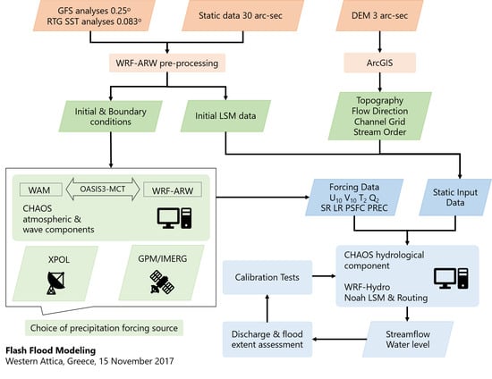
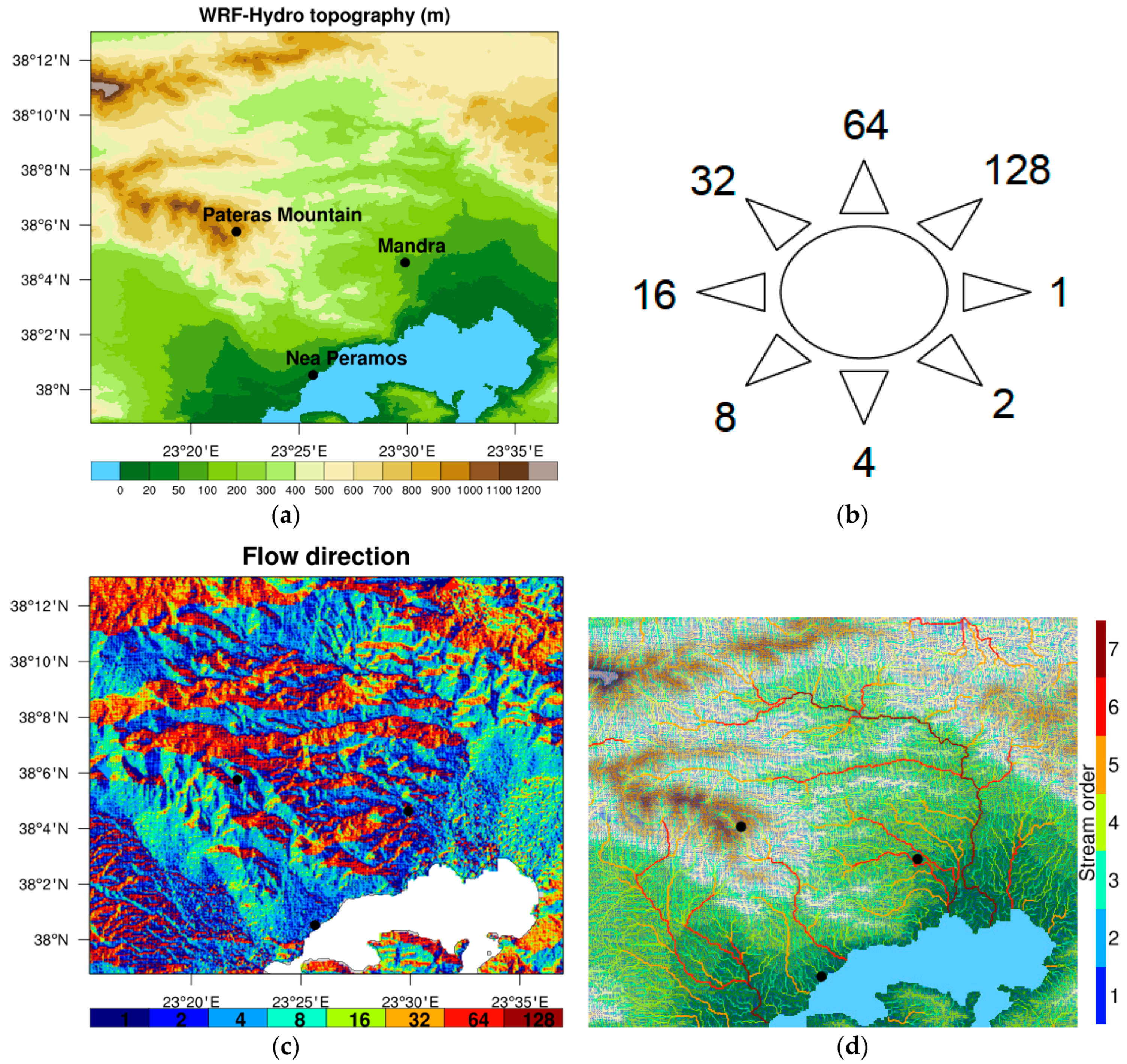
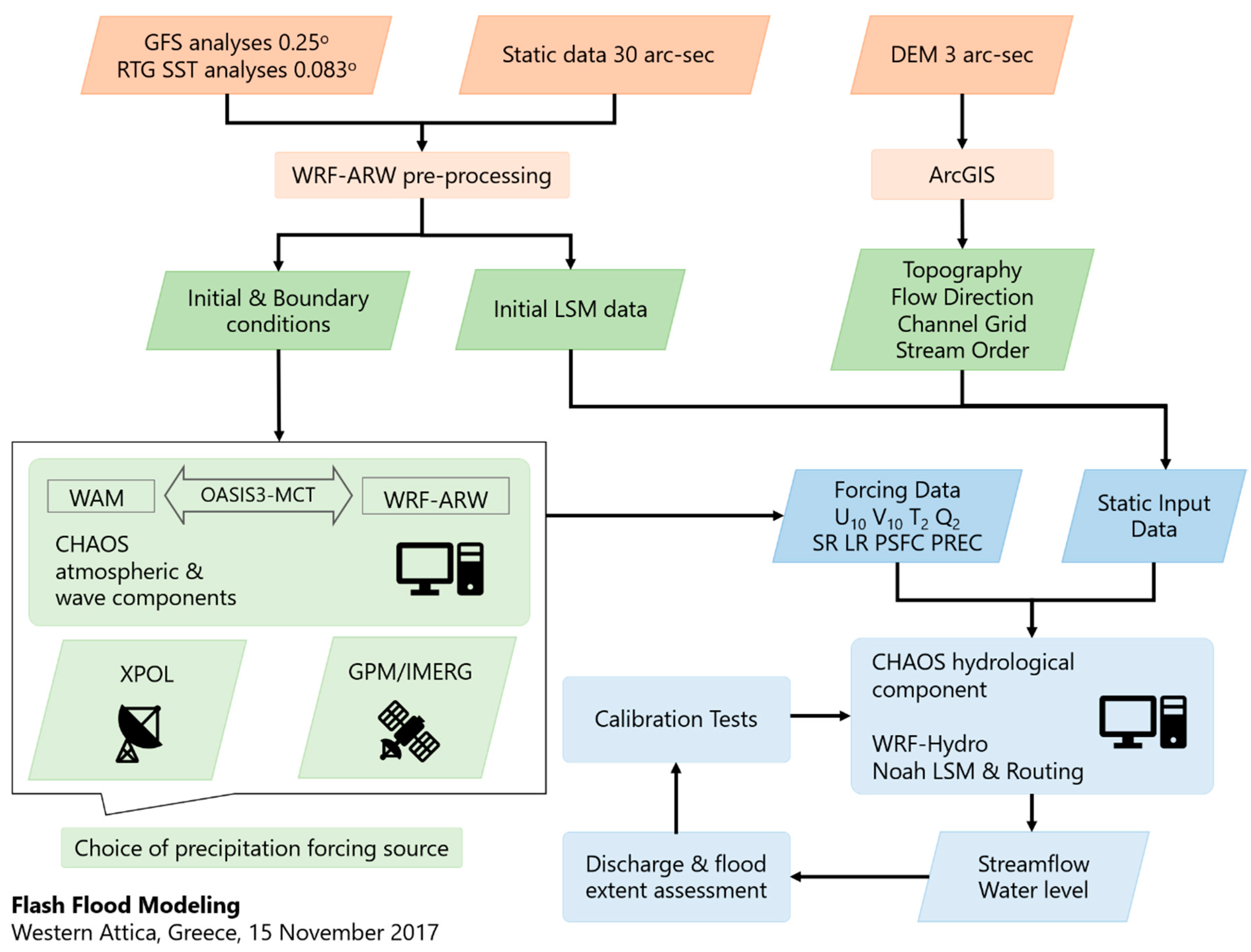
The GPM Core Observatory (CO) is currently the primary rain-measuring satellite equipped with a dual-frequency PR (DPR) (consisting of a Ku-band radar at 13.6 GHz and a Ka-band radar at 35.5 GHz) and the GPM Microwave Imager (GMI), which is a high resolution, conically scanning multichannel (frequencies range 10–183 GHz) MW radiometer [10,63], providing a reference standard to precipitation measurements. The retrieval technique that have been developed, which uses empirical and/or physically-based schemes to estimate precipitation from these satellite observations, are the Integrated Multisatellite Retrievals for Global Precipitation Measurements (IMERG; [64]). The onboard radar on the CO is similar to that on TRMM. The radar scans a swath that is approximately 245 km wide across the satellite track, measuring some 49 footprints of approximately 5 km in diameter and with 250 m vertical resolution at the nadir. The coarsening of the vertical resolution along the distance from the nadir increases from the 250 m up to about 2 km (at 17° from the nadir). The GPM data used in this study is the latest version 5B (V05B) IMERG precipitation product (2.5 months Research/final run) with 0.1° × 0.1° spatial and 30 min temporal resolution. The IMERG is a level 3 gauge-calibrated GPM surface precipitation accumulation estimation product and benefits from the prior precipitation retrieval algorithms including PERSIANN-CCS [65], CMORPH [66], and the TMPA [67].

2.5. Model Set Up

In order to investigate the hydrometeorological characteristics of the flood, the integrated modeling system CHAOS [47,48] is used. The modeling system is configured to perform the simulation from 14 November at 12:00 UTC to 15 November at 12:00 UTC to represent the meteorological conditions during the life-cycle of the severe storm which occurred early in the morning on 15 November. CHAOS consists of two components: the atmospheric model WRF-ARW version 4.0 [40,41] and the ocean wave model WAM version 4.5.4 [68,69]. CHAOS was selected since its atmospheric component offers advanced capabilities in simulating severe weather phenomena [48,70,71,72,73]. The atmospheric component is two-way coupled with the ocean wave component through the OASIS3-MCT version 3.0 coupler [74] to better represent sea surface roughness which plays an important role in the atmospheric surface layer processes offering improvements in forecasting skill [48,75,76,77]. The advantage of CHAOS is the capability to simulate hydrological processes using the WRF-Hydro version 3.0 [36] at defined drainage basins. WRF-Hydro is currently one of the most growing hydrological models. It is noteworthy that WRF-Hydro is used as a framework for connecting atmospheric and hydrologic modeling at the National Water Center of United States [78].
In this study, three experiments using the hydrological component of CHAOS (WRF-Hydro) are performed in order to assess its hydrological response to different precipitation forcing data. The first precipitation dataset is based on the results of the atmospheric component of CHAOS (WRF-ARW), the second on X-band dual-polarization experimental ground radar (XPOL) estimations and the third on GMP/IMERG satellite estimations. CHAOS is configured to produce meteorological forcing fields for the hydrological component with a time step of 1 h. The forcing fields are presented in Table 1. In order to simulate the atmospheric conditions during the flood, the atmospheric component is set up in fine horizontal resolution using multiple nests. This is configured on 4 domains with horizontal resolutions of 9 km × 9 km, 3 km × 3 km, 1 km × 1 km and 0.25 km × 0.25 km (Figure 6). Time steps of 45, 15, 5 and 1 s are employed for the 4 domains, respectively. The initial conditions for 14 November at 12:00 UTC are based on the Global Forecasting System (GFS) operational analyses of the National Centers for Environmental Prediction (NCEP) with a horizontal resolution of 0.25° × 0.25°. The boundary conditions are also based on the GFS operational analyses with a time step of 6 h. The initial sea surface temperature (SST) field is based on the real time global (RTG) SST analyses with a horizontal resolution of 0.083° × 0.083° produced by the NCEP. The Global Multi-resolution Terrain Elevation Data (GMTED 2010 30-arc-sec USGS) [79], the vegetation data MODIS FPAR [80] and the land-use data 21-class IGBP MODIS [81] are used as static input data in the pre-processing stage of WRF model.
The revised Monin–Obukhov scheme [82] is employed to simulate the processes in the atmospheric surface layer, involving a number of modifications to encapsulate wave-dependent sea surface roughness information [47,48]. For the simulation of planetary boundary layer (PBL) processes the Yonsei University scheme (YSU) [65] is used. The ground processes are simulated using the unified Noah land surface model [83]. In order to resolve the long-wave and short-wave radiation processes the rapid radiative transfer model (RRTM) [84] and the Dudhia’s [85] scheme are used, respectively. In order to simulate the microphysics and the convective processes, the Lin [86] and the Grell-Freitas ensemble [87] are used, respectively.
The hydrological model was configured on the extent of the 4th domain of the atmospheric model covering the drainage basin of Mandra on a 5-times finer horizontal resolution (50 m × 50 m). The Shuttle Radar Topographic Mission (SRTM) digital elevation model (DEM) [88] data of NASA in the native horizontal resolution of 90 m × 90 m was used. More specifically, the void-filled version [89] of this dataset distributed by the Hydrological Data and Maps Based on Shuttle Elevation Derivatives at Multiple Scales (HydroSHEDS; https://hydrosheds.cr.usgs.gov/index.php) was selected to be used. The dataset was resampled using nearest-neighbor interpolation on the 50 m × 50 m horizontal grid to introduce information about topography (Figure 7a), flow direction (Figure 7b,c), channel grid and stream order (Figure 7d) in the hydrological model (for more technical details see [36]. Initial conditions for the land surface parameters such as land use, soil type, vegetation, soil moisture and soil temperature required by the land surface model (LSM) NOAH of WRF-Hydro (more information in [36]), were prepared in the pre-processing stage of WRF-ARW model. The land surface data at 30-arc-sec native horizontal resolution was regridded to the grid of the forth domain of WRF-ARW model on horizontal resolution of 250 m × 250 m and, afterwards, to the grid of WRF-Hydro domain at horizontal resolution of 50 m × 50 m. For the two regridding procedures, the bilinear and the nearest-neighbor interpolation methods were used, respectively. As far as land-use is concerned, the USGS 24-category land use categorization was employed.
The hydrographic network (Figure 7d) of the water basin drains surface runoff from the steep mountains to the Thriasio plateau (in the city of Elefsina). In general, the hydrographic network follows a north-south direction, except the Soures and Agia Aikaterini streams (see Figure 2) that initially have a west–east direction and then turns to the north–south direction. A number of smaller streams (5th and 6th order) flowing through the sub-urban area of Elefsina (Figure 7d) drainage from Pateras mountain (Figure 7a) on Sarantapotamos, which functions as the major drainage channel reaching 7th stream order. Sarantapotamos water basin has a length of 31.5 km covering an area of 245.03 km2, surrounded by the mountains Pateras, Pastra (1016 m), Cithaeron (1408 m) and Parnitha (Figure 7d).
For the configuration of the hydrological model, Manning roughness coefficient, channel bottom width, initial water depth and slide slope for channels are set for each stream order as shown in Table 2. These values are chosen after a series of calibration tests which are generally used for a good approximation of river modeling [36]. The initial calibration tests were based on discharge and flood extent assessment.
The hydrographic network of Soures and Agia Aikaterini streams is not monitored at all due to the lack of installed instrumentation. Thus, in order to evaluate the simulated flood extent, post-survey maps created just after the end of the flood event on 15 November and satellite remote sensing images (WorldView-4 in the very high-resolution of 0.31 m) during the period 21–23 November were used; the observed flood extent was mapped by the group of the FloodHub service of BEYOND Center of Excellence for EO-based monitoring of Natural Disasters. The simulated flood extent is delineated using the peak water level along the streams [49]. Regarding the XPOL and Global Precipitation Measurement/Integrated Multi-satellitE Retrievals for GPM (GPM/IMERG) forced hydrological simulations, the water level results on 15 November at 06:00 UTC are used. However, regarding CHAOS forced simulation, the water level results at 03:00 UTC are used because the model predicted the peak of water level 3 h before the 2 other simulations. The topography used for the evaluation procedure is based on the 50 m × 50 m horizontal grid (Figure 7a) produced using nearest-neighbor interpolation for resampling the SRTM DEM 90 m × 90 m data distributed by HydroSHEDS. The interpolation method used for the extraction of the water level surface and consequently the inundated areas is the inverse distance weighted (IDW). Figure 8 illustrates a flowchart summarizing data used, model setup and experimental procedure.

2.6. Evaluation Methodology

Dichotomous forecasts (occurrence or non-occurrence) of the event of interest, in this case a flood, can be considered as “completely confident” forecasts. These forecasts can be treated as categorical forecasts and are usually verified using contingency tables (Table 3) and various scores defined by them [90,91]. A combination of verification measures and scores can be used in comparative evaluation of forecasts, by applying the statistical concept of “sufficiency” [92]. An example of pairs of sufficient statistics for the dichotomous completely confident probability forecasts include probability of detection (PoD) and false alarm ratio (FAR; [93]). In this study, additionally critical success index (CSI) and frequency bias (FB) verification measures was chosen to be included to the evaluation procedure.
The Probability of Detection (PoD or hit rate) and the Critical Success Index (CSI or threat score) range between 0 and 1, with 1 representing a perfect forecast, and can be computed based on Equations (4) and (5), respectively.
PoD = a a + c
CSI = a a + b + c
The FAR ranges between 0 and 1, with 0 representing a perfect forecast. This score is not sensitive to missed events. The FAR can be improved by systematically under forecasting rare events. It also is an incomplete score and should be used in connection with the PoD. FAR can be computed with the following relationship:
FAR = b a + b
The FB is not a true verification measure, as it only compares the forecast and observed frequencies of occurrence of the event in the sample. Frequency bias of 1 represents the best score, values higher than 1 indicate over forecasting and values less than 1 indicate under forecasting. It can be computed using the following relationship [94]:
FB = a + b a + c

3. Results

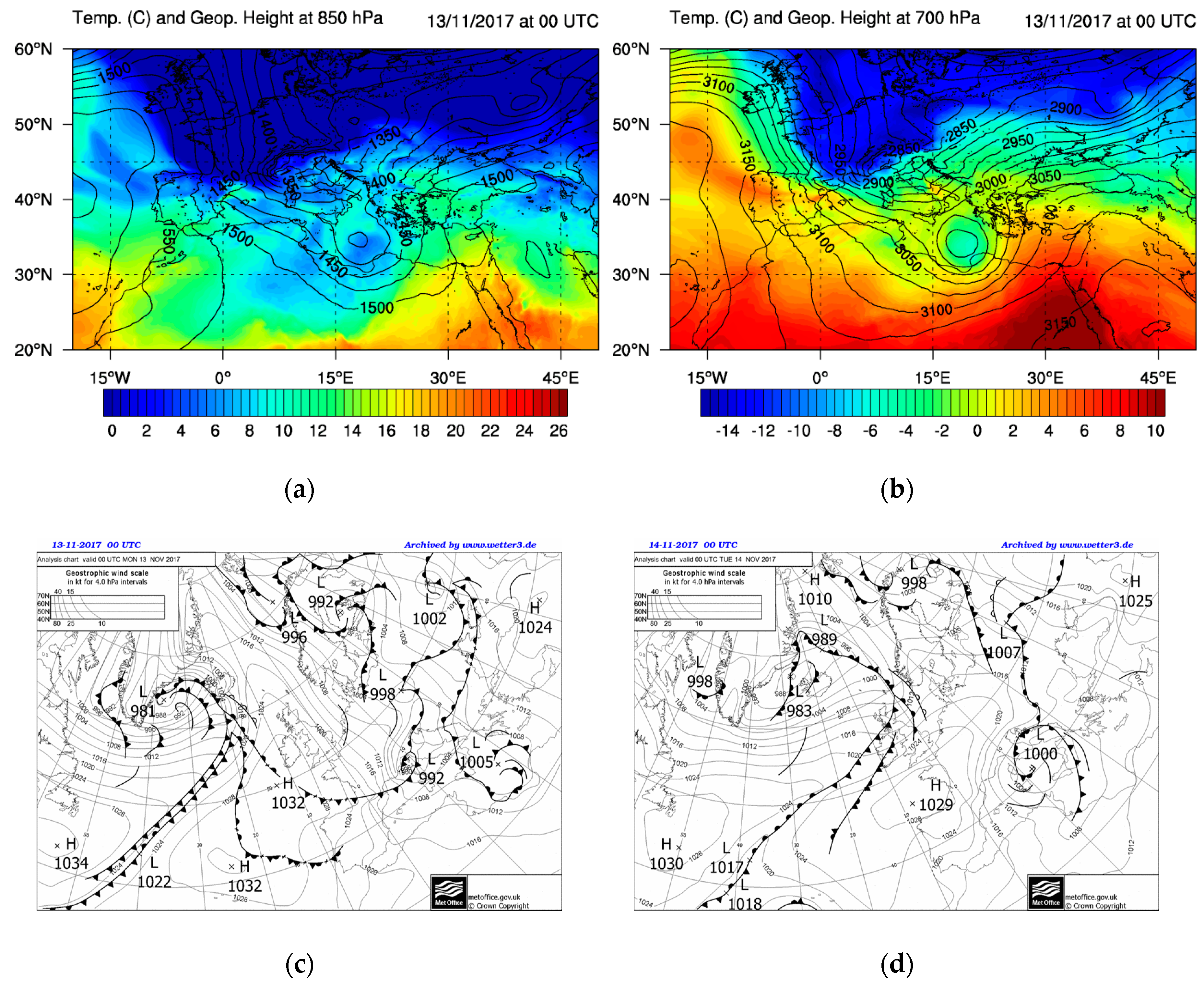
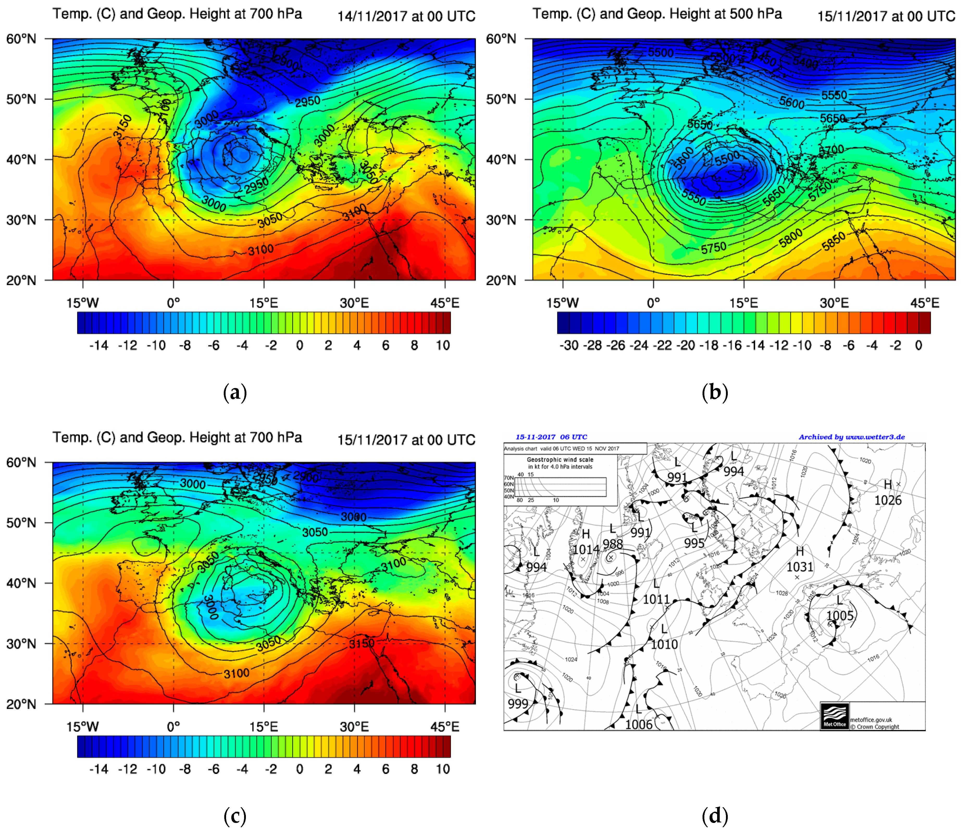
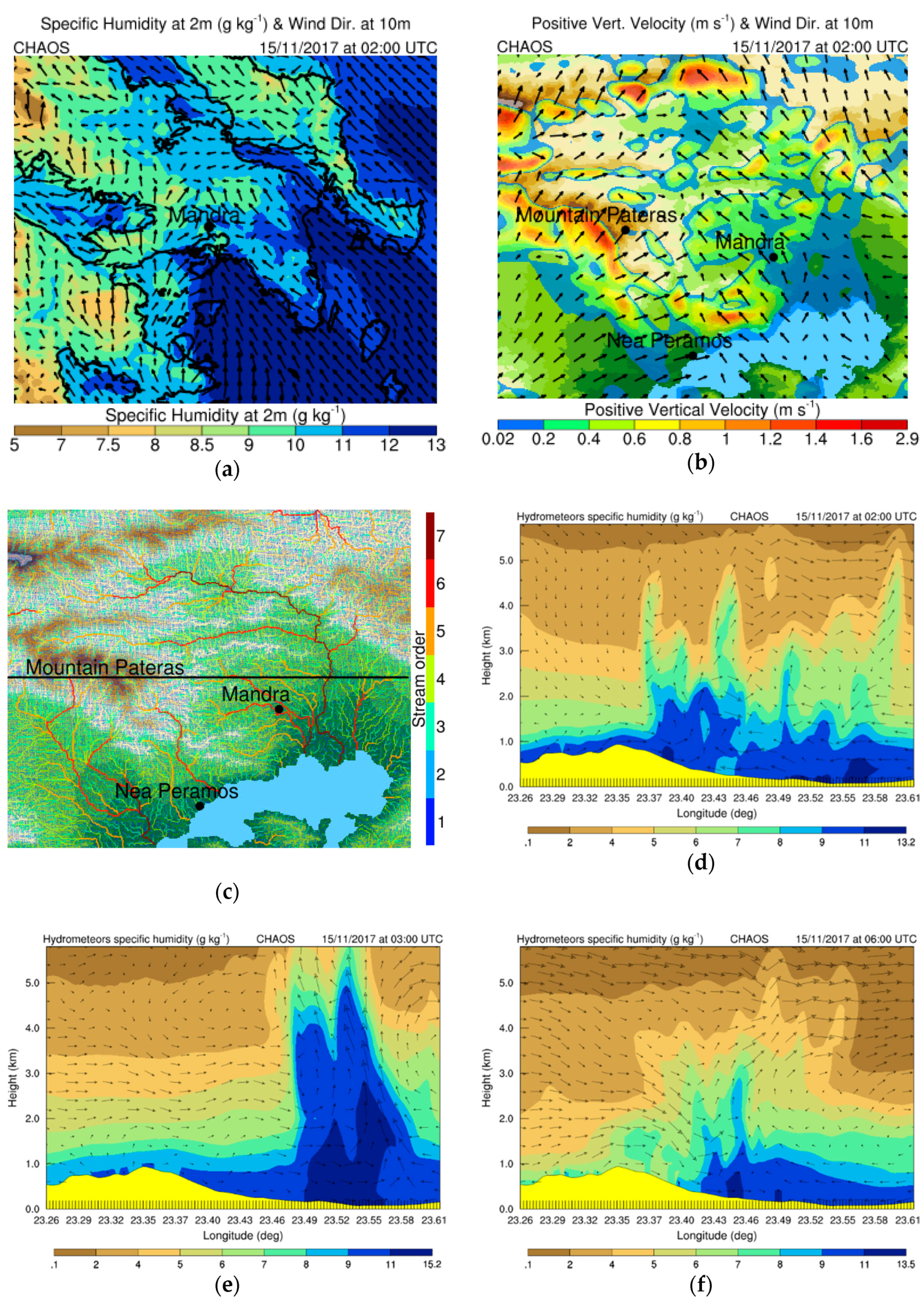
3.1. Meteorological Analysis of the Weather Event

A notable extreme weather event, leading to one of the most devastating flash floods in Attica, occurred on 15 November 2017. The synoptic meteorological conditions over the Mediterranean Sea that led to this destructive flash flood are presented here. On 13 November 2017, a cold air mass was associated with a well-defined trough extending from northwest Europe to the central Mediterranean Sea, as can be seen from the 850 and 700 hPa maps (Figure 9a,b respectively), leading to the generation of a quite deep and extended barometric low centered over northern Italy and a secondary barometric low located to the southeast of Sicily, (Figure 9c). On 14 November, both systems merged into one barometric low over the Tyrrhenian Sea accompanied by widespread warm and cold fronts extending from the Balkan Peninsula to the Gulf of Sirte (Figure 9d).
Subsequently, the barometric system continued to be supported by the upper-level trough. It is important to note that the trough cut off and reinforced the core of the low by introducing very cold air masses over relatively warmer sea (Figure 10a–c). It was stayed almost stagnant during the period from 14 to 19 November under the impact of an upper-air blocking, caused by a well-defined succession of warm air-cold air-warm air (ridge-trough-ridge). This blocking was additionally intensified by the cut-off of the trough forcing the low to stay in place and cause extreme weather phenomena, associated with the floods examined in this study. In the morning of 15 November when the floods at Mandra occurred, the low was well-organized, and it was associated with fronts (Figure 10d).
However, the low and the associated fronts were located far away the flooded area to directly cause storms (Figure 10d). So, it is important to analyze in depth the factors caused such an intense flooding storm. The dominant mechanism is the orographic convergence of humid southeasterly airflow over the southeastern slopes of Pateras mountain (Figure 11a,b). The orographic lifting and the humidity advection are depicted on a vertical cross section up to 6 km for airflow and hydrometeors specific humidity along Pateras mountain and Soures stream head (Figure 11c). Figure 11d–f shows updrafts of humid air over the eastern slopes of Pateras mountain and around Mandra area. The local convergence is collocated with the dry downdrafts over the western slopes of Pateras mountain which are attributed to the middle- and upper-level air circulation. This effect intensified the persistence of rainfall at the east of Pateras mountain increasing surface water runoff and stream discharge as will be shown in the following section. The rainfall was characterized by a long duration of approximately 5 h over this area because it was also indirectly supported by the stagnant spinning barometric low which preserved both the humid southeasterly airflow near the surface and the dry westerly airflow at the middle troposphere. An analysis of the storm focusing on its precipitation characteristics and the hydrological response of the drainage basin of Mandra are presented in the following section.

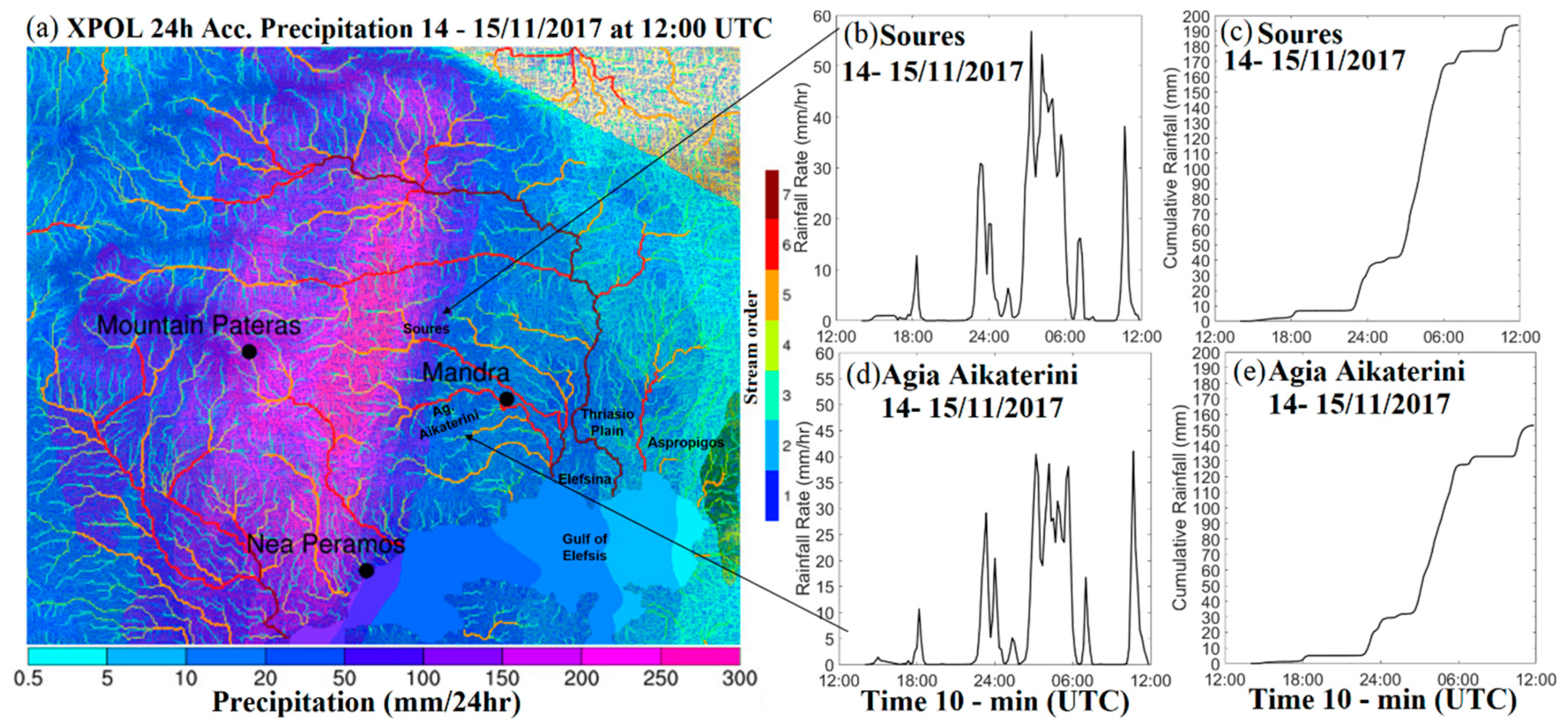
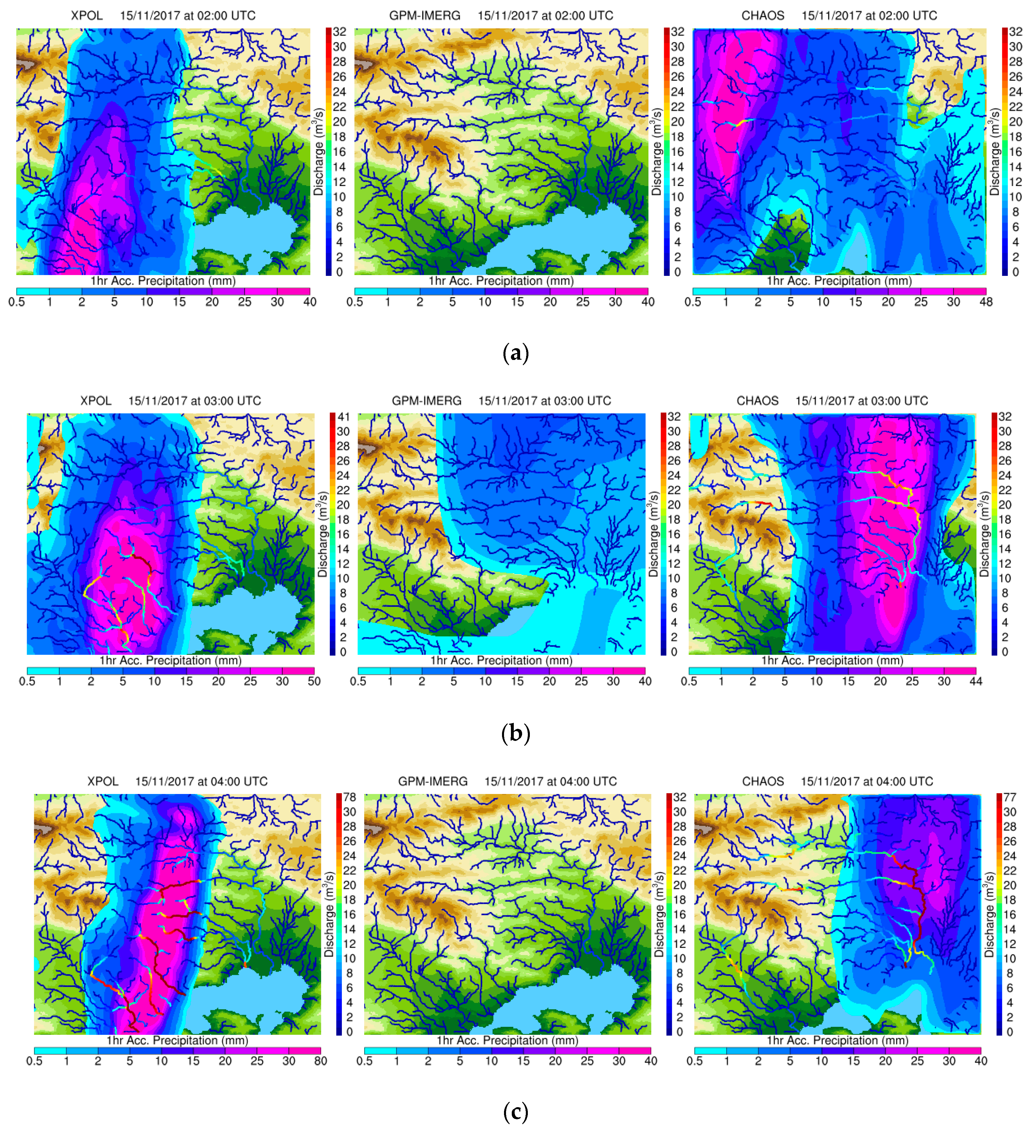
3.2. Quantitative Comparison of Precipitation, Discharge and Water Level

This section presents the quantitative comparison of XPOL, GPM/IMERG and CHAOS precipitation estimates and the respective response of the hydrological model to reproduce the flood event. The high precipitation rates of the 15 November that triggered the high peak runoff at the Agia Aikaterini and Soures streams are analyzed. In addition, this section shows a qualitative comparison between the three different forcing precipitation estimates using hourly simulated discharge maps. Statistics and flood extent maps based on combined simulated data, post-surveys and satellite images as a reference are used.
During the period from 14 November at 12:00 UTC to 15 November at 12:00 UTC, XPOL radar observed up to 300 mm accumulated precipitation in the core of the storm (Figure 12a). During the peak of the storm, from 02:00 to 06:00 UTC, the radar observed basin-average precipitation rates up to 57 mm/h over Soures stream (Figure 12b) and up to 41 mm/h over Agia Aikaterini stream (Figure 12d). Impressive was the fact that the highest precipitation rates in the core of the storm during 02:00–06:00 UTC reached 140 mm/h (not shown here). Moreover, the basin-average 24 h accumulated precipitation reached 194 mm over Soures stream (Figure 12c) and 153 mm over Agia Aikaterini stream (Figure 12e). The local intense rainfall drove the sub-basin network to overflow, flooding the area of Mandra and causing 24 fatalities and extensive million-euro damages to property and infrastructure.
The results of hydrometeorological simulations of the flash flood at western Attica are presented here. Simulated discharge from 02:00 to 04:00 UTC of 15 November is shown in Figure 13a–c, superimposed by the corresponding 1 h accumulated precipitation (mm) estimated by the National Observatory of Athens’ (NOA) XPOL (left), GPM/IMERG (middle) and CHAOS (right). Figure 13 presents different characteristics in the spatial pattern and intensities of the three precipitation estimates, and, subsequently in the simulated discharge. In the case of XPOL precipitation estimate, a persistence over Pateras mountain is observed. This is attributed to the orographic lifting of warm and humid air masses originating from the Aegean Sea (following the southeasterly atmospheric flow which was induced by the stagnant barometric low). It is noteworthy that the spatiotemporal distribution of the precipitation affects the available surface and soil moisture determining surface- and channel-water runoff and, therefore, the streams’ routing [42,43,44]. The relatively increased discharge at Soures and Agia Aikaterini streams at 04:00 UTC presented on the XPOL-hydro simulation is attributed to the increased persistence of intense rainfall over the steep slopes of Pateras mountain (Figure 13c). On the other hand, it seems that the satellite product missed most of the peaks and stage of the storm as it only indicates precipitation at 03:00 UTC (Figure 13b). Yucel et al. [43] also observed an underestimation of WRF-Hydro response on satellite Multi-sensor Precipitation Estimates (MPEs) of EUMETSAT. This may be attributed to poor representation of high precipitation rates by satellites. Possible reasons are the coarse horizontal resolution of satellite data (~11 km for GPM/IMERG and ~4 km for MPEs) which make difficult to capture local extreme weather events as well as various inaccuracies in satellite algorithms. On the other hand, the CHAOS modeling system is closer to the radar precipitation estimates especially in the total duration and the intensity of the rain. An overall comparison of the discharge simulations indicates that the simulation forced by the radar precipitation estimates produced the highest and most accurate in time discharge, which finally led to the flooding.
Concerning the estimated water level, similar outcomes are found from the three differently forced hydrological simulations (Figure 14). Water reaches the level of 130 cm at the Agia Aikaterini and Soures streams when simulated by XPOL-hydro and CHAOS-hydro simulations. However, GPM/IMERG-hydro simulation does not increase water level. Combining Figure 13 and Figure 14, it is obvious that this flash flood event is characterized by a small delay of about 1–2 h after the high precipitation peaks. This is attributed to the limited spatial scale of hydrographic network of the drainage basin of western Attica. Another factor is the high steepness of the eastern slopes of Pateras mountain which accelerates the runoff towards the Agia Aikaterini and Soures streams (see maps in Figure 7).
Simulated discharge and 1 h accumulated precipitation for the period from 05:00 to 07:00 UTC of 15 November are shown in Figure 15. During this period, GPM/IMERG-hydro and CHAOS-hydro simulations underestimate both precipitation and discharge especially at 05:00 UTC when no precipitation was observed or produced. However, CHAOS-hydro has a better performance at Nea Peramos flooding which is not captured by the GPM/IMERG-hydro simulation. XPOL-hydro simulation preserves the storm for hours extending the flooding at Mandra and Nea Peramos areas. XPOL-hydro simulation results in discharge values about 115 m3/s in Soures and Agia Aikaterini streams reaching a peak of 195 m3/s in Sarantapotamos river.
Diakakis et al. [51] estimated a peak discharge for Soures stream about 170 m3/s and for Agia Aikaterini stream about 140 m3/s, using the same XPOL radar rainfall data to force the kinematic local excess model (KLEM; more information in [51]). Diakakis et al. [51] also proposed a semi-empirical method to estimate peak discharge values based on site detailed post-surveys of flood extent and impact, which resulted to wide ranges of peak discharge values (30–40% error based on their analysis) for Soures and Agia Aikaterini streams around the values produced by the KLEM model. The XPOL-based WRF-Hydro simulation is characterized by the minimum difference about 20–30% in the estimated discharge peak with respect to [51]. This difference may be attributed to the configuration of the hydrological models which is usually based on calibration procedures using measured streamflow data [36,43,95,96,97,98] which are not available in this study. It is important to note here that an existing, enclosed rectangular conduit (L = 2.27 km and A = 3.4 m2) in the town has a maximum discharge about 10 m3/s. So, it was inadequate to cope with the extreme discharge during the flash flood event since the minimum required cross sectional area of the streams varies between 20 and 40 m2 [99].
Moreover, Figure 16 shows the simulated water level and 1 h accumulated precipitation for the period from 05:00 to 07:00 UTC of 15 November. During this period, XPOL-hydro simulates water level exceeding 300 cm in Agia Aikaterini and Soures streams as well as in Sarantapotamos river. CHAOS-hydro estimates approximately half the water levels having a good agreement with XPOL-hydro. GPM/IMERG-hydro simulates a weak increase of water level.
Figure 17a depicts the hydrographic and stream order map of the water basin where black dots represent the points used to make hydrograph of each simulation for the period from 14 November at 12:00 UTC to 15 November at 12:00 UTC (Figure 17b). P1 is used to export 1 h accumulated precipitation from the XPOL dataset, while P2 is used for GPM/IMERG and CHAOS datasets. Different points are used here to represent the precipitation maxima of the three datasets avoiding in that manner mismatches of the pattern and the phase speed of the barometric low. P3 is used to export discharge from the datasets that resulted from all three hydrological simulations. As shown in Figure 17b, GPM/IMERG data systematically estimate much less precipitation compared to XPOL while CHAOS hourly precipitation is closer to the XPOL one. The increased underestimation of the GPM/IMERG, comparing to the XPOL and CHAOS, is mainly attributed to its coarser resolution which did not support enough representation of such a local extreme precipitation event. In addition, due to the lack of passive microwave or radar data in this specific area at the time of the event the IMERG algorithm uses interpolation of available data following the feature motion which is estimated from infrared satellite data. As far as the discharge is concerned, CHAOS matches better with the XPOL radar estimations in comparison to the satellite which does not cause flooding. The differences between CHAOS and XPOL precipitation data are attributed to forecast inaccuracies of numerical weather prediction.
As far as streams’ overflow is concerned, Soures and Agia Aikaterini were not enough to carry the extremely high discharges and they overflowed [49]. Various public infrastructure and private constructions were erected over the two streams while the necessary water drainage pipes were either too small or they were not built at all [100]. One of the reasons for the extensive damage during the flood event was the human interference on Mandra’s streams (see Figure 2). Moreover, the artificially confined channels of the streams and the drainage pipes were inefficient at facilitating the flow of the run-off water [99]. As a result, the flood additionally caused significant soil erosion by carrying away large quantities of sediment particles due to high flow and stream-bottom shear stresses. Fine sand, silt and clay of considerable thickness were deposited along the roads of Mandra as well as at the mouth of the streams along the shoreline of the Gulf of Elefsina, indicating the high sediment load of the drainage networks during the event [50]. Additionally, debris and heavy objects, such as cars and trees were carried away by the torrents. The large amounts of solid materials transported by the streams may have resulted in an additional rise of the water level in the streams.

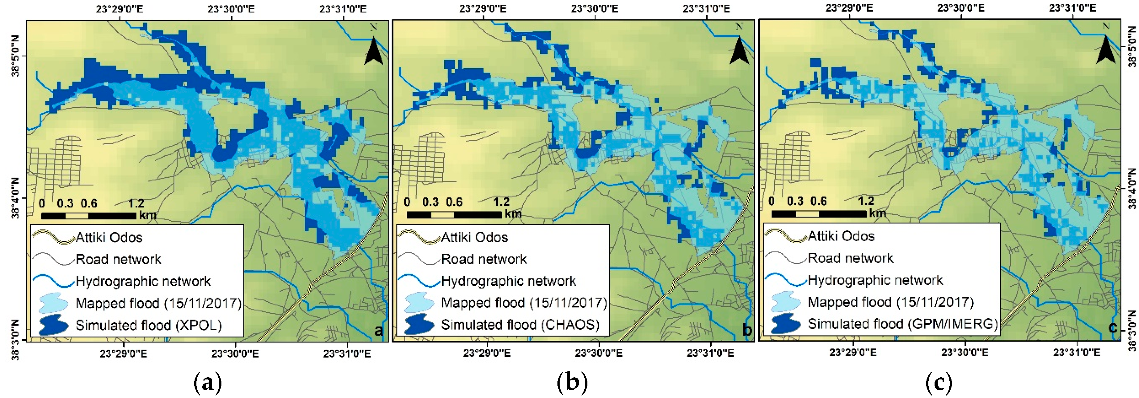
3.3. Qualitative Evaluation of Estimated Flood Extent

In this section a comparison of simulated and observed flood extent is presented. Due to the high inaccuracies of the flooded areas estimation, the assessment of flood extent is qualitative. The evaluation is restricted to the area upstream of the “Attiki Odos” highway (Figure 18), the construction of which has altered the hydro-morphological characteristics of the area but simultaneously provides adequate flood protection at most of the adjacent areas [101]. Only the 6th and 7th order streams are used during this analysis, while the upstream areas are not included in the analysis.
Based on the evaluation of the different statistical scores that are summarized in Table 4, the best PoD score was accomplished by the XPOL rainfall estimation forcing to the hydrological model (0.66), meaning that 66% of the observed flooded area was correctly predicted. The worst PoD score was accomplished by the GPM/IMERG-hydro (0.30). The higher CSI score was again accomplished by XPOL (0.43), indicating that less than half of the flooded area (observed and/or predicted) was correctly forecasted. The worst CSI score was again accomplished by the GPM/IMERG-hydro (0.24). FAR score was practically identical among the three experiments confirming in that manner their similar capabilities to simulate flooded areas that failed to materialize. FAR scores (0.43–0.45) indicate that in less than the half-flooded area simulated, flood was eventually not observed. The FB score was greater than 1 in the case of XPOL-hydro, indicating over-forecast, and lower than 1 in the cases of CHAOS-hydro and GPM/IMERG-hydro, indicating under-forecast, especially in the case of GPM/IMERG-hydro. Overall, XPOL-hydro managed to predict the flood event with satisfactory accuracy, although it over estimated the inundated area (Figure 18a). CHAOS-hydro showed a marginally acceptable skill to simulate the flooded areas despite the fact of the significant uncertainties and forecast errors usually posed by the numerical weather prediction models (Figure 18b). GPM/IMERG-hydro, on the other hand, did not predict the flood event accurately and under estimated the flooded area (Figure 18c).
Possible inaccuracies affected the entire set of simulations can be attributed to the coarse resolution of the digital elevation map (DEM), which does not allow the extraction of detailed cross sections along the streams. Especially upstream where the riverbeds are narrow, the flooded areas could not be predicted with accuracy due to the lack of detailed information concerning the geometry of the streams. It should be also noted that the flood took place in an extremely dense urban fabric that was not properly designed. This information was not possible to be included in the simulation in detail.

4. Discussion

The comparison of the results of the three hydrological simulations reveals XPOL and CHAOS precipitation forcing data estimated water level and discharge in a more efficient way than GMP/IMERG data. The rapid increase of these hydrological parameters indicated a flash flood event, which is attributed to the persistence of high precipitation rates over the steep slopes of Pateras mountain for approximately 5 h (as observed by the XPOL radar). Basin-average precipitation rates reached 57 mm/h over Soures stream, 41 mm/h over Agia Aikaterini stream and 140 mm/h in the core of the storm. Moreover, the XPOL-radar observed 24 h accumulated precipitation up to 300 mm in the core of the storm. Time series of basin-average accumulated precipitation for the two sub-basins of Soures and Agia Aikaterini streams indicated high cumulative precipitation reaching 194 mm and 153 mm, respectively. CHAOS-hydro estimated approximately the half water levels and even lower discharges compared to XPOL-hydro simulation, while, having good agreement in the representation of spatial and temporal characteristics of the storm, and, subsequently of the flooding event. GPM/IMERG-hydro simulated a weak increase of water level and discharge due to the low precipitation estimation. It is noteworthy that XPOL-hydro simulation resulted in discharge values about 115 m3/s and water level values exceeding 3 m in Soures and Agia Aikaterini streams which caused the flash flooding around the Mandra area.
It is difficult to make a comprehensive representation of reference discharge during this flood event, due to lack of instrumentation. Diakakis et al. [51] proposed a semi-empirical method to estimate peak discharge values based on site detailed post-surveys of flood extent and impact, which yielded relatively broad ranges of peak discharge values (30–40% error) for Soures and Agia Aikaterini streams around the values produced by the KLEM model forced by the same XPOL radar rainfall estimates. More specifically, Diakakis et al. [51] estimated a peak discharge for Soures stream about 170 m3/s and for Agia Aikaterini stream about 140 m3/s. All the three experiments based on WRF-Hydro underestimated discharge peak compared with KLEM results. The XPOL-hydro simulation is characterized by the minimum difference in the estimation of discharge peak per 20–30% in respect to the KLEM estimation. The differences may be attributed to inaccuracies in the precipitation estimates and the configuration of the hydrological model, which demands high calibration effort [36,43,96,97,98] using measurements which are not available at this area. Moreover, an explanation for the dominance of the XPOL-hydro simulation is the higher spatial and temporal resolution of precipitation estimates (120 m and 3 min) than the respective resolutions of CHAOS (250 m and 1 h) and GPM/IMERG (~11 km and 30 min) precipitation datasets.
The combination of the increased volume of run-off water with the human pressures on the streams interrupting their flow caused wide flood extent. The flash flood affected almost the entire town of Mandra [49]. Comparing with the observed flooded areas, the XPOL-hydro simulation presented overestimation. On the other hand, GPM/IMERG-hydro did not predict the flood event accurately and underestimated the flooded area while CHAOS-hydro showed sufficient skill to simulate the flooded areas despite the forecast inaccuracies of numerical weather prediction.
Another reason for the extensive damage during this flood event was the fact that the artificially confined channels of the streams and the drainage pipes were inefficient at facilitating the run-off water. An existing, enclosed rectangular conduit with capability of discharge about 10 m3/s was inadequate to cope with the extreme discharge during the flash flood event [99]. Moreover, the streets of Mandra sometimes played the role of the streams of Soures and Agia Aikaterini concentrating large quantities of water and sediments.

5. Conclusions

The aim of this work is to perform a hydrometeorological analysis of the extreme flash flood event of the 15 November 2017 at the sub-urban area of Mandra, western Attica, Greece, applying an integrated remote sensing and data-modeling system. The flood event occurred at Soures and Agia Aikaterini streams and affected the suburban town of Mandra with landslides, extensive damage and a total of 24 fatalities.
This case study has been simulated by the integrated modeling system CHAOS including an advanced hydrological model (WRF-Hydro) able to offer improved simulation of land surface hydrology in a fine spatial resolution. Analyzing CHAOS meteorological results, an intense storm over Pateras mountain during the morning of 15 November resulted in a tremendous flooding event. The dominant meteorological mechanism for this storm was the orographic convergence of warm and humid southeasterly airflow over the steep slopes of Pateras mountain which caused persistent rainfall and increased the volume of surface run-off water. This effect was characterized by a long duration of approximately 5 h over this area as it was indirectly supported by an almost stagnant spinning Mediterranean cyclone over the Tyrrhenian and Ionian Seas.
The WRF-Hydro model simulated this case study using three different precipitation forcing datasets. The first was based on CHAOS hindcasts (CHAOS-hydro), the second one was based on XPOL radar precipitation estimates (XPOL-hydro) and the third one, on GMP/IMERG estimated precipitation rates (GMP/IMERG-hydro). The XPOL precipitation forcings were evaluated against surface rain gauge and disdrometer observations close to the area of interest with encouraging results. The comparison of the precipitation estimation with in situ rain gauge observations revealed high correlations (~0.90) and bias ratio around 10% with a normalized error of 5%.
Overall, the findings of this study from the hydrologic simulations demonstrate the potential benefit of using high-resolution observations from a locally deployed X-band dual-polarization radar as an additional forcing component in model precipitation simulations. The use of X-band weather radars is rapidly increasing with the advance of technology and data correction and processing algorithms, as well as their reduced costs for installation and maintenance with respect to the operational long-range C- and S-band systems. The high resolution and the increased sensitivity of X-band radars make them quite suitable for nowcasting purposes [102,103,104]. The range limitation of X-band radars due to the larger attenuation in rain in this microwave band can be surpassed using radar networks, whose setup improves also the accuracy of radar products [105,106,107].
In future, radar data assimilation in CHAOS modeling system and radar tracking algorithms, which are available for operational radars but are equally applied to X-band radars [103], can be implemented for nowcasting purposes, supporting better estimations of both atmospheric and hydrological characteristics during flash flooding situations.

Author Contributions

G.V., M.N.A. and C.S. contributed to the methodology, formal analysis, investigation, visualization and writing-original draft preparation; A.P., J.K., A.M. and S.M. contributed to the methodology, investigation, writing, review and editing; E.B. and E.K. contributed to the methodology and investigation; P.K. contributed to the conceptualization, methodology, supervision, investigation, review and editing.

Funding

This research received no external funding.

Acknowledgments

The Greek Research and Technology Network (GRNET) is gratefully acknowledged for the access to the high-performance computer (HPC) ARIS (https://hpc.grnet.gr/), where the simulations of this study have been performed. The National Centers for Environmental Prediction (NCEP) is gratefully acknowledged for the provision of the Global Forecasting System (GFS) operational analyses and the real time global (RTG) sea surface temperature (SST) analyses. The National Aeronautics and Space Administration (NASA) and the Hydrological Data and Maps Based on Shuttle Elevation Derivatives at Multiple Scales (HydroSHEDS) are fruitfully acknowledged for the kind provision of the Shuttle Radar Topographic Mission (SRTM) digital elevation model (DEM) data. UK Met Office and www1.wetter3.de are gratefully acknowledged for the kind provision of surface analysis maps.

Conflicts of Interest

The authors declare no conflict of interest.

References

  1. Hirabayashi, Y.; Mahendran, R.; Koirala, S.; Konoshima, L.; Yamazaki, D.; Watanabe, S.; Kim, H.; Kanae, S. Global flood risk under climate change. Nat. Clim. Chang. 2013, 3, 816–821. [Google Scholar] [CrossRef]
  2. Kundzewicz, Z.W.; Mata, L.J.; Arnell, N.W.; Döll, P.; Kabat, P.; Jiménez, B.; Miller, K.A.; Oki, T.; Sen, Z.; Shiklomanov, I.A. Freshwater Resources and Their Management. Climate Change 2007: Impacts, Adaptation and Vulnerability. Contribution of Working Group II to the Fourth Assessment Report of the Intergovernmental Panel on Climate Change; Parry, M.L., Canziani, O.F., Palutikof, J.P., van der Linden, P.J., Hanson, C.E., Eds.; Cambridge University Press: Cambridge, UK, 2007; pp. 173–210. [Google Scholar]
  3. Meehl, G.A.; Arblaster, J.M.; Tebaldi, C. Understanding future patterns of precipitation extremes in climate model simulations. Geophys. Res. Lett. 2005, 32, L18719. [Google Scholar] [CrossRef]
  4. Conti, F.L.; Hsu, K.L.; Noto, L.V.; Sorooshian, S. Evaluation and comparison of satellite precipitation estimates with reference to a local area in the Mediterranean sea. Atmos. Res. 2014, 138, 189–204. [Google Scholar] [CrossRef]
  5. Dinku, T.; Anagnostou, E.N.; Borga, M. Improving radar-based estimation of rainfall over complex terrain. J. Appl. Meteorol. 2002, 41, 1163–1178. [Google Scholar] [CrossRef]
  6. Derin, Y.; Anagnostou, E.N.; Anagnostou, M.N.; Kalogiros, J.; Casella, D.; Marra, A.C.; Panegrossi, G.; Sanò, P. Passive microwave rainfall error analysis using high-resolution X-band dual-polarization radar observations in complex terrain. IEEE Trans. Geosci. Remote Sens. 2018, 56, 2565–2586. [Google Scholar] [CrossRef]
  7. Anagnostou, M.N.; Kalogiros, J.; Anagnostou, E.N.; Papadopoulos, A. Experimental results on rainfall estimation in complex terrain with a mobile X-band polarimetric radar. Atmos. Res. 2009, 94, 579–595. [Google Scholar] [CrossRef]
  8. Wang, Y.; Chandrasekar, V. Quantitative precipitation estimation in the CASA X-band dual-polarization radar network. J. Atmos. Ocean. Technol. 2010, 27, 1665–1676. [Google Scholar] [CrossRef]
  9. Matrosov, S.Y.; Cifelli, R.; Gochis, D. Measurements of heavy convective rainfall in the presence of hail in flood-prone areas using an X-band polarimetric radar. J. Appl. Meteorol. Climatol. 2013, 52, 395–407. [Google Scholar] [CrossRef]
  10. Koffi, A.K.; Gosset, M.; Zahiri, E.-P.; Ochou, A.D.; Kacou, M.; Cazenave, F.; Assamoi, P. Evaluation of X-band polarimetric radar estimation of rainfall and rain drop size distribution parameters in West Africa. Atmos. Res. 2014, 143, 438–461. [Google Scholar] [CrossRef]
  11. Vulpiani, G.; Baldini, L.; Roberto, N. Characterization of Mediterranean hail-bearing storms using an operational polarimetric X-band radar. Atmos. Meas. Tech. 2015, 8, 4681–4698. [Google Scholar] [CrossRef]
  12. Anagnostou, M.N.; Nikolopoulos, E.I.; Kalogiros, J.; Anagnostou, E.N.; Marra, F.; Mair, E.; Bertoldi, G.; Tappeiner, U.; Borga, M. Advancing precipitation estimation and streamflow simulations in complex terrain with X-band dual-polarization radar observations. Remote Sens. 2018, 10, 1258. [Google Scholar] [CrossRef]
  13. Chandrasekar, V.; Chen, H.; Philips, B. DFW urban radar network observations of floods, tornadoes and hail storms. In Proceedings of the IEEE Radar Conference, Oklahoma City, OK, USA, 23–27 April 2018; pp. 765–770. [Google Scholar]
  14. Shakti, P.C.; Maki, M.; Shimizu, S.; Maesaka, T.; Kim, D.; Lee, D.; Iida, H. Correction of Reflectivity in the Presence of Partial Beam Blockage over a Mountainous Region Using X-Band Dual Polarization Radar. J. Hydrometeorol. 2013, 14, 744–764. [Google Scholar]
  15. Chen, H.; Chandrasekar, V. The quantitative precipitation estimation system for Dallas-Fort Worth (DFW) urban remote sensing network. J. Hydrol. 2015, 531, 259–271. [Google Scholar] [CrossRef]
  16. Tobin, K.J.; Bennett, M.E. Adjusting satellite precipitation data to facilitate hydrologic modeling. J. Hydrometeorol. 2010, 11, 966–978. [Google Scholar] [CrossRef]
  17. Cohen Liechti, T.; Matos, J.P.; Boillat, J.L.; Schleiss, A.J. Comparison and evaluation of satellite derived precipitation products for hydrological modeling of the Zambezi River Basin. Hydrol. Earth Syst. Sci. 2012, 16, 489–500. [Google Scholar] [CrossRef]
  18. Anagnostou, E.N. Overview of overland satellite rainfall estimation for hydro-meteorological applications. Surv. Geophys. 2004, 25, 511–537. [Google Scholar] [CrossRef]
  19. Hou, A.Y.; Kakar, R.K.; Neeck, S.; Azarbarzin, A.A.; Kummerow, C.D.; Kojima, M.; Oki, R.; Nakamura, K.; Iguchi, T. The global precipitation measurement mission. Bull. Am. Meteorol. Soc. 2014, 95, 701–722. [Google Scholar] [CrossRef]
  20. Gaume, E.; Borga, M.; Llassat, M.C.; Maouche, S.; Lang, M.; Diakakis, M. Mediterranean extreme floods and flash floods. In The Mediterranean Region under Climate Change—A Scientific Update. IRD Editions; Coll. Synthèses: Marseille, France, 2016; pp. 133–144. ISBN 978-2-7099-2219-7. Available online: https://hal.archives-ouvertes.fr/hal-01465740/document (accessed on 29 November 2018).
  21. Camarasa-Belmonte, A.; Segura, F. Flood events in Mediterranean ephemeral streams (ramblas) in Valencia region, Spain. Catena 2001, 45, 229–249. [Google Scholar] [CrossRef]
  22. Llasat, M.C.; Marcos, R.; Turco, M.; Gilabert, J.; Llasat-Botija, M. Trends in flash flood events versus convective precipitation in the Mediterranean region: The case of Catalonia. J. Hydrol. 2016, 541, 24–37. [Google Scholar] [CrossRef]
  23. Runge, J.; Nguimalet, C.R. Physiogeographic features of the Oubangui catchment and environmental trends reflected in discharge and floods at Bangui 1911–1999, Central African Republic. Geomorphology 2005, 70, 311–324. [Google Scholar] [CrossRef]
  24. Papagiannaki, K.; Lagouvardos, K.; Kotroni, V. A database of high-impact weather events in Greece: A descriptive impact analysis for the period 2001–2011. Nat. Hazards Earth Syst. Sci. 2013, 13, 727–736. [Google Scholar] [CrossRef]
  25. Wallace, J.M.; Hobbs, P.V. Atmospheric Science: An Introductory Survey, 2nd ed.; Academic Press: Cambridge, MA, USA, 2006; ISBN 978-0-12-732951-2. [Google Scholar]
  26. Morel, C.; Senesi, S. A climatology of mesoscale convective systems over Europe using satellite infrared imagery. II. Characteristics of European mesoscale convective systems. Q. J. R. Meteorol. Soc. 2002, 128, 1973–1995. [Google Scholar] [CrossRef]
  27. Kolios, S.; Feidas, H. A warm season climatology of mesoscale convective systems in the Mediterranean basin using satellite data. Theor. Appl. Climatol. 2010, 102, 29–42. [Google Scholar] [CrossRef]
  28. Despiniadou, V.; Athanasopoulou, E. Flood prevention and sustainable spatial planning. The case of the river Diakoniaris in Patras. In Proceedings of the 46th Congress of the European Regional Science Association (ERSA), Volos, Greece, 30 August–3 September 2006; Available online: https://www.econstor.eu/bitstream/10419/118466/1/ERSA2006_672.pdf (accessed on 9 November 2018).
  29. Diakakis, M.; Mavroulis, S.; Deligiannakis, G. Floods in Greece, a statistical and spatial approach. Nat. Hazards 2012, 62, 485–500. [Google Scholar] [CrossRef]
  30. Baltas, E.A.; Mimikou, M.A. Considerations for the optimum location of a C-band weather radar in the Athens area. In Proceedings of the 3rd European Conference on radar Meteorology and Hydrology, ERAD 2002, Delft, The Netherlands, 18–22 November 2002; pp. 348–351. Available online: https://www.copernicus.org/erad/online/erad-348.pdf (accessed on 9 November 2018).
  31. Skilodimou, H.; Livaditis, G.; Bathrellos, G.; Verikiou-Papaspiridakou, E. Investigating the flooding events of the urban regions of Glyfada and Voula, Attica, Greece: A contribution to Urban Geomorphology. Geogr. Ann. A 2003, 85, 197–204. [Google Scholar] [CrossRef]
  32. Mimikou, M.; Baltas, E.; Varanou, E. A Study of Extreme Storm Events in the Greater Athens Area, Greece. The Extremes of the Extremes, Extraordinary Floods; IAHS-AISH Publication: Reykjavik, Iceland, 2002; Volume 271, pp. 161–166. [Google Scholar]
  33. Karymbalis, E.; Katsafados, P.; Chalkias, C.; Gaki-Papanastassiou, K. An integrated study for the evaluation o of natural and anthropogenic causes of flooding in small catchments based on geomorphological and meteorological data and modeling techniques: The case of the Xerias torrent (Corinth, Greece). Z. Geomorphol. 2012, 56, 45–67. [Google Scholar] [CrossRef]
  34. Mazi, K.; Koussis, A.D. The 8 July 2002 storm over Athens: Analysis of the Kifissos River/Canal overflows. Adv. Geosci. 2006, 7, 301–306. [Google Scholar] [CrossRef]
  35. Papagiannaki, K.; Kotroni, V.; Lagouvardos, K.; Ruin, I.; Bezes, A. Urban areas response to flash flood-triggering rainfall, featuring human behavioural factors: The case of 22 October 2015, in Attica, Greece. Weather Clim. Soc. 2017, 9, 621–638. [Google Scholar] [CrossRef]
  36. Gochis, D.J.; Yu, W.; Yates, D.N. The WRF-Hydro Model Technical Description and User’s Guide, version 3.0; NCAR Technical Document; NCAR: Boulder, CO, USA, 2015; Available online: https://ral.ucar.edu/sites/default/files/public/images/project/WRF_Hydro_User_Guide_v3.0.pdf (accessed on 9 November 2018).
  37. Giannoni, F.; Roth, G.; Rudari, R. A semi-distributed rainfall–runoff model based on a geomorphologic approach. Phys. Chem. Earth B 2000, 25, 665–671. [Google Scholar] [CrossRef]
  38. Shen, X.; Hong, Y.; Zhang, K.; Hao, Z.; Wang, D. CREST v2.1 Refined by a Distributed Linear Reservoir Routing Scheme. In Proceedings of the American Geophysical Union, Fall Meeting 2014, San Francisco, CA, USA, 15–19 December 2014. abstract #H33G-0918. [Google Scholar]
  39. Seity, Y.; Brousseau, P.; Malardel, S.; Hello, G.; Benard, P.; Bouttier, F.; Lac, C.; Masson, V. The AROME–France convective-scale operational model. Mon. Weather Rev. 2011, 139, 976–991. [Google Scholar] [CrossRef]
  40. Skamarock, W.C.; Klemp, J.B.; Dudhia, J.; Gill, D.O.; Barker, D.M.; Dudha, M.G.; Huang, X.; Wang, W.; Powers, Y. A Description of the Advanced Research WRF Ver. 3.0; NCAR Technical Note; NCAR: Boulder, CO, USA, 2008; Available online: http://www2.mmm.ucar.edu/wrf/users/docs/arw_v3.pdf (accessed on 9 November 2018).
  41. Powers, J.G.; Klemp, J.B.; Skamarock, W.C.; Davis, C.A.; Dudhia, J.; Gill, D.O.; Coen, J.L.; Gochis, D.J.; Ahmadov, R.; Peckham, S.E.; et al. The weather research and forecasting model: Overview, system efforts, and future directions. Bull. Am. Meteorol. Soc. 2017, 98, 1717–1737. [Google Scholar] [CrossRef]
  42. Senatore, A.; Mendicino, G.; Gochis, D.J.; Yu, W.; Yates, D.N.; Kunstmann, H. Fully coupled atmosphere-hydrology simulations for the central Mediterranean: Impact of enhanced hydrological parameterization for short and long time scales. J. Adv. Model. Earth Syst. 2015, 7, 1693–1715. [Google Scholar] [CrossRef]
  43. Yucel, I.; Onen, A.; Yilmaz, K.K.; Gochis, D.J. Calibration and evaluation of a flood forecasting system: Utility of numerical weather prediction model, data assimilation and satellite-based rainfall. J. Hydrol. 2015, 523, 49–66. [Google Scholar] [CrossRef]
  44. Givati, A.; Gochis, D.; Rummler, T.; Kunstmann, H. Comparing one-way and two-way coupled hydrometeorological forecasting systems for flood forecasting in the Mediterranean region. Hydrology 2016, 3, 19. [Google Scholar] [CrossRef]
  45. Berne, A.; Delrieu, G.; Creutin, J.; Obled, C. Temporal and spatial resolution of rainfall measurements required for urban hydrology. J. Hydrol. 2004, 299, 166–179. [Google Scholar] [CrossRef]
  46. Atencia, A.; Mediero, L.; Llasat, M.C.; Garrote, L. Effect of radar rainfall time resolution on the predictive capability of a distributed hydrologic model. Hydrol. Earth Syst. Sci. 2011, 15, 3809–3827. [Google Scholar] [CrossRef]
  47. Varlas, G. Development of an Integrated Modeling System for Simulating the Air-Ocean Wave Interactions. Ph.D. Dissertation, Harokopio University of Athens (HUA), Athens, Greece, 2017. Available online: https://www.didaktorika.gr/eadd/handle/10442/41238 (accessed on 9 November 2018).
  48. Varlas, G.; Katsafados, P.; Papadopoulos, A.; Korres, G. Implementation of a two-way coupled atmosphere-ocean wave modeling system for assessing air-sea interaction over the Mediterranean Sea. Atmos. Res. 2018, 208, 201–217. [Google Scholar] [CrossRef]
  49. FloodHub. Analysis of the Flood in Western Attica on 15/11/2017 Using Satellite Remote Sensing. Available online: http://www.beyond-eocenter.eu/images/news-events/20180430/Mandra-Report-BEYOND.pdf (accessed on 29 November 2018). (In Greek).
  50. Environmental, Disasters and Crises Management (EDCM). Flash Flood in West Attica (Mandra, Nea Peramos) Newsletter #5. 15 November 2017. Available online: http://www.elekkas.gr/index.php/en/epistimoniko-ergo/edcm-newsletter/1603-edcm-newsletter-5-flash-flood-in-west-attica-mandra-nea-peramos-november-15-2017 (accessed on 9 November 2018).
  51. Diakakis, M.; Andreadakis, E.; Spyrou, N.I.; Gogou, M.E.; Nikolopoulos, E.I.; Deligiannakis, G.; Katsetsiadou, N.K.; Antoniadis, Z.; Melaki, M.; Georgakopoulos, A.; et al. The flash flood of Mandra 2017, in West Attica, Greece—Description of impacts and flood characteristics. Int. J. Disaster Risk Reduct. 2018. [Google Scholar] [CrossRef]
  52. Katsafados, P.; Kalogirou, S.; Papadopoulos, A.; Korres, G. Mapping long-term atmospheric variables over Greece. J. Maps 2012, 8, 181–184. [Google Scholar] [CrossRef]
  53. Mavrakis, A.; Theoharatos, G.; Asimakopoulos, D.; Christides, A. Distribution of the trace metals in sediments of Eleusis Gulf. Mediterr. Mar. Sci. 2004, 5, 151–158. [Google Scholar] [CrossRef]
  54. Institute of Geology and Mineral Exploration (IGME). Geological Map of Greece (scale 1:50,000), Sheet Erithrai. 1971. Available online: http://portal.igme.gr/geoportal/ (accessed on 9 November 2018).
  55. Kalogiros, J.; Anagnostou, M.N.; Anagnostou, E.N.; Montopoli, M.; Picciotti, E.; Marzano, F.S. Optimum estimation of rain microphysical parameters using X-band dual-polarization radar observables. IEEE Trans. Geosci. Remote Sens. 2013, 51, 3063–3076. [Google Scholar] [CrossRef]
  56. Anagnostou, M.N.; Kalogiros, J.; Anagnostou, E.N.; Tarolli, M.; Papadopoulos, A.; Borga, M. Performance evaluation of high-resolution rainfall estimation by X-band dual-polarization radar for flash flood applications in mountainous basin. J. Hydrol. 2010, 394, 4–16. [Google Scholar] [CrossRef]
  57. Kalogiros, J.; Anagnostou, M.N.; Anagnostou, E.N.; Montopoli, M.; Picciotti, E.; Marzano, F.S. Correction of polarimetric radar reflectivity measurements and rainfall estimates for apparent vertical profile in stratiform rain. J. Appl. Meteorol. Climatol. 2013, 52, 1170–1186. [Google Scholar] [CrossRef]
  58. Kalogiros, J.; Anagnostou, M.N.; Anagnostou, E.N.; Montopoli, M.; Picciotti, E.; Marzano, F.S. Evaluation of a new polarimetric algorithm for rain-path attenuation correction of X-band radar observations against disdrometer. IEEE Trans. Geosci. Remote Sens. 2014, 52, 1369–1380. [Google Scholar] [CrossRef]
  59. Anagnostou, M.N.; Kalogiros, J.; Marzano, F.S.; Anagnostou, E.N.; Montopoli, M.; Picciotti, E. Performance evaluation of a new dual-polarization microphysical algorithm based on long-term X-band radar and disdrometer observations. J. Hydrometeorol. 2013, 14, 560–576. [Google Scholar] [CrossRef]
  60. Habib, E.; Krajewski, W.F.; Kruger, A. Sampling errors of tipping bucket rain gauge measurements. J. Hydrol. Eng. 2001, 6, 159–166. [Google Scholar] [CrossRef]
  61. Porcacchia, L.; Kirstetter, P.-E.; Gourley, J.J.; Maggioni, V.; Cheong, B.L.; Anagnostou, M.N.; Kalogiros, J. Toward a radar polarimetric classification scheme for warm-rain precipitation: Application to complex terrain. J. Hydrometeorol. 2017, 18, 3199–3215. [Google Scholar] [CrossRef]
  62. Erlingis, J.M.; Gourley, J.J.; Kirstetter, P.-E.; Anagnostou, E.N.; Kalogiros, J.; Anagnostou, M.N.; Peterseni, W. Evaluation of operational and experimental precipitation algorithms and microphysical insights during IPHEx. J. Hydrometeorol. 2018, 19, 113–125. [Google Scholar] [CrossRef]
  63. Sun, Q.; Miao, C.; Duan, Q.; Ashouri, H.; Sorooshian, S.; Hsu, K.-L. A review of global precipitation datasets: Data sources, estimation, and intercomparisons. Rev. Geophys. 2018, 56, 79–107. [Google Scholar] [CrossRef]
  64. Huffman, G.J.; Bolvin, D.T.; Braithwaite, D.; Hsu, K.L.; Joyce, R.; Xie, P. NASA Global Precipitation Measurement (GPM) Integrated Multi-Satellite Retrievals for GPM (IMERG); Algorithm Theor. Basis Doc. (ATBD) Version 5.1; NASA GSFC: Greenbelt, MD, USA, 2014. Available online: https://pmm.nasa.gov/sites/default/files/document_files/IMERG_ATBD_V5.1b.pdf (accessed on 9 November 2018).
  65. Hong, Y.; Hsu, K.L.; Sorooshian, S.; Gao, X. Precipitation estimation from remotely sensed imagery using an Artificial Neural Network cloud classification system. J. Appl. Meteorol. 2004, 43, 1834–1852. [Google Scholar] [CrossRef]
  66. Joyce, R.J.; Janowiak, J.E.; Arkin, P.A.; Xie, P. CMORPH: A method that produces global precipitation estimates from passive microwave and infrared data at high spatial and temporal resolution. J. Hydrometeorol. 2004, 5, 487–503. [Google Scholar] [CrossRef]
  67. Huffman, G.J.; Bolvin, D.T.; Nelkin, E.J.; Wolff, D.B.; Adler, R.F.; Gu, G.; Hong, Y.; Bowman, K.P.; Stocker, E.F. The TRMM Multisatellite Precipitation Analysis (TMPA): Quasi-global, multiyear, combined-sensor precipitation estimates at fine scales. J. Hydrometeorol. 2007, 8, 38–55. [Google Scholar] [CrossRef]
  68. Hasselmann, S.; Hasselmann, K.; Bauer, E.; Janssen, P.A.E.M.; Komen, G.J.; Bertotti, L.; Lionello, P.; Guillaume, A.; Cardone, V.C.; Greenwood, J.A.; et al. The WAM model—A third generation ocean wave prediction model. J. Phys. Oceanogr. 1988, 18, 1775–1810. [Google Scholar] [CrossRef]
  69. Komen, G.J.; Cavaleri, L.; Donelan, M.; Hasselmann, K.; Hasselmann, S.; Janssen, P.A.E.M. Dynamics and Modeling of Ocean Waves; Cambridge University Press: Cambridge, UK, 1994. [Google Scholar]
  70. Christakos, K.; Varlas, G.; Reuder, J.; Katsafados, P.; Papadopoulos, A. Analysis of a low-level coastal jet off the western coast of Norway. Energy Procedia 2014, 53, 162–172. [Google Scholar] [CrossRef]
  71. Christakos, K.; Cheliotis, I.; Varlas, G.; Steeneveld, G.J. Offshore wind energy analysis of cyclone Xaver over North Europe. Energy Procedia 2016, 94, 37–44. [Google Scholar] [CrossRef]
  72. Cheliotis, I.; Varlas, G.; Christakos, K. The impact of cyclone Xaver on hydropower potential in Norway. In Perspectives on Atmospheric Sciences; Springer: Cham, Germany, 2017; pp. 175–181. [Google Scholar]
  73. Varlas, G.; Papadopoulos, A.; Katsafados, P. An analysis of the synoptic and dynamical characteristics of hurricane Sandy (2012). Meteorol. Atmos. Phys. 2018, 1–11. [Google Scholar] [CrossRef]
  74. Valcke, S.; Craig, T.; Coquart, L. OASIS3-MCT_3.0 Coupler User Guide; CERFACS/CNRS: Toulouse, France, 2015; Available online: http://www.cerfacs.fr/oa4web/oasis3-mct_3.0/oasis3mct_UserGuide.pdf (accessed on 9 November 2018).
  75. Katsafados, P.; Papadopoulos, A.; Korres, G.; Varlas, G. A fully coupled atmosphere-ocean wave modeling system for the Mediterranean Sea: Interactions and sensitivity to the resolved scales and mechanisms. Geosci. Model Dev. 2016, 9. [Google Scholar] [CrossRef]
  76. Katsafados, P.; Varlas, G.; Papadopoulos, A.; Korres, G. Implementation of a Hybrid Surface Layer Parameterization Scheme for the Coupled Atmosphere-Ocean Wave System WEW. In Perspectives on Atmospheric Sciences; Springer: Cham, Germany, 2017; pp. 159–165. [Google Scholar]
  77. Katsafados, P.; Varlas, G.; Papadopoulos, A.; Spyrou, C.; Korres, G. Assessing the implicit rain impact on sea state during hurricane Sandy (2012). Geophys. Res. Lett. 2018, 45, 12015–12022. [Google Scholar] [CrossRef]
  78. Maidment, D.R. Conceptual framework for the national flood interoperability experiment. J. Am. Water Resour. Assoc. 2017, 53, 245–257. [Google Scholar] [CrossRef]
  79. Danielson, J.J.; Gesch, D.B. Global Multi-Resolution Terrain Elevation Data 2010 (GMTED2010) (No. 2011-1073); US Geological Survey: Reston, VA, USA, 2011. Available online: https://pubs.er.usgs.gov/publication/ofr20111073 (accessed on 9 November 2018).
  80. Myneni, R.B.; Hoffman, S.; Knyazikhin, Y.; Privette, J.L.; Glassy, J.; Tian, Y.; Wang, Y.; Song, X.; Zhang, Y.; Smith, G.R.; et al. Global products of vegetation leaf area and fraction absorbed PAR from year one of MODIS data. Remote Sens. Environ. 2002, 83, 214–231. [Google Scholar] [CrossRef]
  81. Friedl, M.A.; Sulla-Menashe, D.; Tan, B.; Schneider, A.; Ramankutty, N.; Sibley, A.; Huang, X. MODIS Collection 5 global land cover: Algorithm refinements and characterization of new datasets. Remote Sens. Environ. 2010, 114, 168–182. [Google Scholar] [CrossRef]
  82. Jiménez, P.A.; Dudhia, J.; González-Rouco, J.F.; Navarro, J.; Montávez, J.P.; García-Bustamante, E. A revised scheme for the WRF surface layer formulation. Mon. Weather Rev. 2012, 140, 898–918. [Google Scholar] [CrossRef]
  83. Tewari, M.; Chen, F.; Wang, W.; Dudhia, J.; LeMone, M.A.; Mitchell, K.; Gayno, G.; Wegiel, J.; Cuenca, R.H. Implementation and verification of the unified NOAH land surface model in the WRF model. In Proceedings of the 20th Conference on Weather Analysis and Forecasting/16th Conference on Numerical Weather Prediction, Seattle, WA, USA, 12–16 January 2004; pp. 2165–2170. Available online: https://ams.confex.com/ams/84Annual/techprogram/paper_69061.htm (accessed on 9 November 2018).
  84. Mlawer, E.J.; Taubman, S.J.; Brown, P.D.; Iacono, M.J.; Clough, S.A. Radiative transfer for inhomogeneous atmospheres: RRTM, a validated correlated-k model for the longwave. J. Geophys. Res. Atmos. 1997, 102, 16663–16682. [Google Scholar] [CrossRef]
  85. Dudhia, J. Numerical study of convection observed during the winter monsoon experiment using a mesoscale two-dimensional model. J. Atmos. Sci. 1989, 46, 3077–3107. [Google Scholar] [CrossRef]
  86. Lin, Y.-L.; Farley, R.D.; Orville, H.D. Bulk Parameterization of the Snow Field in a Cloud Model. J. Clim. Appl. Met. 1983, 22, 1065–1092. [Google Scholar] [CrossRef]
  87. Grell, G.A.; Freitas, S.R. A scale and aerosol aware stochastic convective parameterization for weather and air quality modeling. Atmos. Chem. Phys. 2014, 14, 5233–5250. [Google Scholar] [CrossRef]
  88. Jarvis, A.; Reuter, H.I.; Nelson, A.; Guevara, E. Hole-Filled SRTM for the Globe Version 4. CGIAR-CSI SRTM 90m Database. Available online: http://srtm.csi.cgiar.org (accessed on 9 November 2018).
  89. Lehner, B.; Verdin, K.; Jarvis, A. New global hydrography derived from spaceborne elevation data. Eos Trans. Am. Geophys. Union 2008, 89, 93–94. [Google Scholar] [CrossRef]
  90. Wilks, D.S. Statistical Methods in the Atmospheric Sciences; Academic Press: Cambridge, MA, USA, 2011. [Google Scholar]
  91. Wilson, L.J. Verification of Precipitation Forecasts: A Survey of Methodology. Part I: General Framework and Verification of Continuous Variables. In Proceedings of the WWRP/WMO Workshop on the Verification of Quantitative Precipitation Forecasts, Prague, Czech Republic, 14–16 May 2001. [Google Scholar]
  92. Ehrendorfer, M.; Murphy, A.H. Comparative evaluation of weather forecasting systems: Sufficiency, quality, and accuracy. Mon. Weather Rev. 1988, 116, 1757–1770. [Google Scholar] [CrossRef]
  93. Brown, B.G. Verification of Precipitation Forecasts: A Survey of Methodology. Part II: Verification of Probability Forecasts at Points. In Proceedings of the WWRP/WMO Workshop on the Verification of Quantitative Precipitation Forecasts, Prague, Czech Republic, 14–16 May 2001. [Google Scholar]
  94. World Meteorological Organization. Forecast Verification for the African Severe Weather Forecasting Demonstration Projects; No. 1132; World Meteorological Organization: Geneva, Switzerland, 2014; Available online: https://www.wmo.int/pages/prog/www/Documents/1132_en.pdf (accessed on 9 November 2018).
  95. Arnault, J.; Wagner, S.; Rummler, T.; Fersch, B.; Bliefernicht, J.; Andresen, S.; Kunstmann, H. Role of runoff–infiltration partitioning and resolved overland flow on land–atmosphere feedbacks: A case study with the WRF-Hydro coupled modeling system for West Africa. J. Hydrometeorol. 2016, 17, 1489–1516. [Google Scholar] [CrossRef]
  96. Krajewski, W.F.; Ceynar, D.; Demir, I.; Goska, R.; Kruger, A.; Langel, C.; Mantilla, R.; Niemeier, J.; Quintero, F.; Seo, B.C.; et al. Real-time flood forecasting and information system for the state of Iowa. Bull. Am. Meteorol. Soc. 2017, 98, 539–554. [Google Scholar] [CrossRef]
  97. Ryu, Y.; Lim, Y.J.; Ji, H.S.; Park, H.H.; Chang, E.C.; Kim, B.J. Applying a coupled hydrometeorological simulation system to flash flood forecasting over the Korean Peninsula. Asia-Pacific. J. Atmos. Sci. 2017, 53, 421–430. [Google Scholar] [CrossRef]
  98. Silver, M.; Karnieli, A.; Ginat, H.; Meiri, E.; Fredj, E. An innovative method for determining hydrological calibration parameters for the WRF-Hydro model in arid regions. Environ. Model. Softw. 2017, 91, 47–69. [Google Scholar] [CrossRef]
  99. Stamou, A.I. The disastrous flash flood of Mandra in Attica-Greece and now what? Civ. Eng. Res. J. 2018, 6, 1–6. [Google Scholar] [CrossRef]
  100. Greek City Times. Local Authorities and Bureaucracy Blamed for Mandra Floods. Available online: https://greekcitytimes.com/2017/12/29/local-authorities-bureaucracy-blamed-mandra-floods (accessed on 9 November 2018).
  101. Serbis, D.; Papathanasiou, C.; Mamassis, N. Mitigating flooding in a typical urban area in North Western Attica in Greece. In Proceedings of the Conference on Changing Cities: Spatial Design, Landscape and Socio-economic Dimensions, Porto Heli, Peloponnese, Greece, 22–26 June 2015; Available online: http://www.itia.ntua.gr/en/getfile/1563/1/documents/P588-Changing_Cities2015_Full_paper.pdf (accessed on 9 November 2018).
  102. Picciotti, E.; Marzano, F.S.; Anagnostou, E.N.; Kalogiros, J.; Fessas, Y.; Volpi, A.; Cazac, V.; Pace, R.; Cinque, G.; Bernardini, L.; et al. Coupling X-band dual-polarized mini-radar and hydro-meteorological forecast models: The HYDRORAD project. Nat. Hazards Earth Syst. Sci. 2013, 13, 1229–1241. [Google Scholar] [CrossRef]
  103. Conti, F.L.; Francipane, A.; Pumo, D.; Noto, L.V. Exploring single polarization X-band weather radar potentials for local meteorological and hydrological applications. J. Hydrol. 2015, 531, 508–522. [Google Scholar] [CrossRef]
  104. Shah, S.; Notarpietro, R.; Branca, M. Storm identification, tracking and forecasting using high-resolution images of short-range X-Band radar. Atmosphere 2015, 6, 579–606. [Google Scholar] [CrossRef]
  105. McLaughlin, D.; Pepyne, D.; Chandrasekar, V.; Philips, B.; Kurose, J.; Zink, M.; Droegemeier, K.; Cruz-Pol, S.; Junyent, F.; Brotzge, J.; et al. Short-wavelength technology and the potential for distributed networks of small radar systems. Bull. Am. Meteorol. Soc. 2009, 90, 1797–1817. [Google Scholar] [CrossRef]
  106. Chandrasekar, V.; Wang, Y.; Chen, H. The CASA quantitative precipitation estimation system: A five year validation study. Nat. Hazards Earth Syst. Sci. 2012, 12, 2811–2820. [Google Scholar] [CrossRef]
  107. Lengfeld, K.; Clemens, M.; Munster, H.; Ament, F. Performance of high-resolution X-band weather radar networks—The PATTERN example. Atmos. Meas. Tech. 2014, 7, 4151–4166. [Google Scholar] [CrossRef]
Figure 1. Map of study area depicting Thriasio Plateau among Pateras, Parnitha and Aigaleo mountains and the towns of Mandra, Nea Peramos and Elefsina. Source: Google Maps.
Remotesensing 11 00045 g001
Figure 2. (a) Aerial photo taken in 1945 (Hellenic Military Geographical Service); (b) 2018 Google Earth image of the broader area of the city of Mandra showing the natural channels of streams Soures and Agia Aikaterini.
Remotesensing 11 00045 g002
Figure 3. (a) Topographic map of the area covered from the X-band dual polarization (XPOL) radar encompassing (the shading circle) the experimental basin, the in situ instruments, and the town of Mandra. Pictures from the deployed sensors are also shown; (b) at the upper right is the XPOL radar; (c) meteorological station with the Parsivel disdrometer at the National Technical University of Athens (NTUA) site.
Remotesensing 11 00045 g003
Figure 4. Τime series of precipitation rate (mm/10min) from the three different in situ sites used for the evaluation of the XPOL precipitation algorithm. The dashed line indicates the flash flood event took place on 15 November 2017.
Remotesensing 11 00045 g004
Figure 5. The scatterplot of XPOL hourly precipitation estimates versus the three rain gauge observations, where the “1-1” line is the bold black line.
Remotesensing 11 00045 g005
Figure 6. Chemical Hydrological Atmospheric Ocean Wave System (CHAOS) domains and topography (m). The nested domains of atmospheric component are depicted with red polygons and the domain of the wave component with blue polygon.
Remotesensing 11 00045 g006
Figure 7. (a) hydrological model WRF-Hydro 50 m × 50 m topography and three areas represented by black dots: Pateras mountain, Mandra and Nea Peramos; (b) flow direction discretization. The flow direction grid has integer values of 1, 2, 4, 8, 16, 32, 64 and 128 which are oriented in the depicted directions; (c) flow direction; (d) hydrographic and stream order map of the water basin used for the hydrological runs.
Remotesensing 11 00045 g007
Figure 8. Flowchart of data used, model configuration and experimental procedure. Data, parameters and models are thoroughly described in the text.
Remotesensing 11 00045 g008
Figure 9. Temperature and geopotential height based on Global Forecasting System (GFS) analyses for 13 November 2017 (00:00 UTC) at: (a) 850 hPa and (b) 700 hPa. UK Met Office surface analysis maps on: (c) 13 November 2017 (00:00 UTC) and (d) 14 November 2017 (00:00 UTC).
Remotesensing 11 00045 g009
Figure 10. (a) Temperature and geopotential height based on GFS analyses for 14 November 2017 (00:00 UTC) at 700 hPa; temperature and geopotential height on 15 November 2017 (00:00 UTC) at (b) 500 hPa and (c) 700 hPa; (d) UK Met Office surface analysis map for 15 November 2017 (06:00 UTC).
Remotesensing 11 00045 g010
Figure 11. (a) Specific humidity at 2 m and horizontal wind vectors at 10 m; (b) positive vertical velocity and horizontal wind vectors at 10 m (on the right) on 15 November 2017 (02:00 UTC); The two maps (a,b) are based on CHAOS simulation results obtained from the third and fourth nested domains, respectively. (c) Hydrographic and stream order map of the water basin illustrating the vertical cross section area (black line). Vertical cross section up to 6 km for hydrometeors specific humidity (g kg−1) and wind on 15 November 2017 at (d) 02:00 UTC, (e) 03:00 UTC and (f) 06:00 UTC based on CHAOS simulation results obtained from the fourth nested domain.
Remotesensing 11 00045 g011
Figure 12. (a) Hydrographic and stream order map of the water basin with superimposed the XPOL 24 h precipitation accumulation; Time series of basin-average (b) precipitation rate and (c) accumulated precipitation for Soures stream; Time series of basin-average (d) precipitation rate and (e) accumulated precipitation for Agia Aikaterini stream. Figures refer to the period from 14 November at 12:00 UTC to 15 November at 12:00 UTC.
Remotesensing 11 00045 g012
Figure 13. 1 h accumulated precipitation estimations from the National Observatory of Athens’ (NOA) XPOL radar (left), the Global Precipitation Measurement/Integrated Multi-satellitE Retrievals for GPM (GPM/IMERG) (middle) and CHAOS (right). On the same maps the simulated discharges forced from each of the three precipitation estimations are superimposed. Only streams with order higher than 4 are presented. The maps refer to 15 November at (a) 02:00, (b) 03:00 and (c) 04:00 UTC.
Remotesensing 11 00045 g013
Figure 14. 1 h accumulated precipitation estimations from the NOA’s XPOL radar (left), the GPM/IMERG (middle) and CHAOS (right). On the same maps the simulated water levels forced from each of the three precipitation estimations are superimposed. Only streams with order higher than 4 are presented. The maps refer to 15 November at (a) 02:00, (b) 03:00 and (c) 04:00 UTC.
Remotesensing 11 00045 g014
Figure 15. 1 h accumulated precipitation estimations from the NOA’s XPOL radar (left), the GPM/IMERG (middle) and CHAOS (right). On the same maps the simulated discharges forced from each of the three precipitation estimations are superimposed. Only streams with order higher than 4 are presented. The maps refer to 15 November at (a) 05:00, (b) 06:00 and (c) 07:00 UTC.
Remotesensing 11 00045 g015
Figure 16. 1 h accumulated precipitation estimations from the NOA’s XPOL radar (left), the GPM/IMERG (middle) and CHAOS (right). On the same maps the simulated water levels forced from each of the three precipitation estimations are superimposed. Only streams with order higher than 4 are presented. The maps refer to 15 November at (a) 05:00, (b) 06:00 and (c) 07:00 UTC.
Remotesensing 11 00045 g016
Figure 17. (a) Hydrographic and stream order map of the water basin as Figure 7d. Black dots represent the points used for the time series. P1 is used to export 1 h accumulated precipitation from XPOL dataset, while P2 is respectively used for GPM/IMERG and CHAOS datasets. P3 is used to export discharge from the datasets that resulted from all the three hydrological simulations. (b) Hydrograph: time series of 1 h accumulated precipitation and discharge estimations using XPOL radar, the GPM/IMERG and CHAOS forcing on hydrological model.
Remotesensing 11 00045 g017
Figure 18. Flood extent produced by the three hydrological simulations (dark blue) using precipitation forcing by: (a) XPOL; (b) CHAOS; (c) GPM/IMERG datasets. Flood extent mapped by the FloodHub group of BEYOND (Building a Centre of Excellence for Earth Observation-based monitoring of Natural Disasters) project during the 15 November flood event (light blue).
Remotesensing 11 00045 g018
Table 1. The seven meteorological forcing fields [34].
Meteorological Forcing FieldsUnits
Incoming shortwave radiation (SR)(W/m2)
Incoming longwave radiation (LR)(W/m2)
Air specific humidity at 2 m (Q2)(kg/kg)
Air temperature at 2 m (T2)(K)
Surface pressure (PSFC)(Pa)
Near surface wind at 10 m in the u- and v-components (U10, V10)(m/s)
Liquid water precipitation rate (PREC)(mm/s)
Table 2. Manning roughness coefficient (Manning), channel bottom width (CBW) in m, initial water depth (IWD) in m and slide slope (CSS) of channels for each stream order.
Stream OrderManningCBW (m)IWD (m)CSS
10.310.051.0
20.320.050.8
30.2530.10.6
40.240.10.4
50.1560.10.2
60.180.20.1
70.05100.20.05
Table 3. Contingency table for evaluation.
Simulated EventObserved Event
YesNo
YesHit (a)False alarm (b)
NoMiss (c)Correct non-event (d)
Table 4. Results of the scores used for the validation of the three hydrological simulations.
XPOL-HydroCHAOS-HydroGPM/IMERG-Hydro
PoD0.660.430.30
CSI0.430.330.24
FAR0.450.430.43
FB1.210.750.53

