The Assessment of Landsat-8 OLI Atmospheric Correction Algorithms for Inland Waters


1
Key Laboratory of Watershed Geographic Sciences, Nanjing Institute of Geography & Limnology Chinese Academy of Sciences, Nanjing 210008, China
2
University of Chinese Academy of Sciences, Beijing 100049, China
3
Dipartimento di Biotecnologie, Chimica e Farmacia, University of Siena, CSGI, Via Aldo Moro 2, 53100 Siena, Italy
*
Author to whom correspondence should be addressed.
Remote Sens. 2019, 11(2), 169; https://0-doi-org.brum.beds.ac.uk/10.3390/rs11020169
Submission received: 29 November 2018
/
Revised: 12 January 2019
/
Accepted: 15 January 2019
/
Published: 17 January 2019
(This article belongs to the Special Issue Satellite Monitoring of Water Quality and Water Environment)
Abstract
:The OLI (Operational Land Imager) sensor on Landsat-8 has the potential to meet the requirements of remote sensing of water color. However, the optical properties of inland waters are more complex than those of oceanic waters, and inland atmospheric correction presents additional challenges. We examined the performance of atmospheric correction (AC) methods for remote sensing over three highly turbid or hypereutrophic inland waters in China: Lake Hongze, Lake Chaohu, and Lake Taihu. Four water-AC algorithms (SWIR (Short Wave Infrared), EXP (Exponential Extrapolation), DSF (Dark Spectrum Fitting), and MUMM (Management Unit Mathematics Models)) and three land-AC algorithms (FLAASH (Fast Line-of-sight Atmospheric Analysis of Spectral Hypercubes), 6SV (a version of Second Simulation of the Satellite Signal in the Solar Spectrum), and QUAC (Quick Atmospheric Correction)) were assessed using Landsat-8 OLI data and concurrent in situ data. The results showed that the EXP (and DSF) together with 6SV algorithms provided the best estimates of the remote sensing reflectance (Rrs) and band ratios in water-AC algorithms and land-AC algorithms, respectively. AC algorithms showed a discriminating accuracy for different water types (turbid waters, in-water algae waters, and floating bloom waters). For turbid waters, EXP gave the best Rrs in visible bands. For the in-water algae and floating bloom waters, however, all water-algorithms failed due to an inappropriate aerosol model and non-zero reflectance at 1609 nm. The results of the study show the improvements that can be achieved considering SWIR bands and using band ratios, and the need for further development of AC algorithms for complex aquatic and atmospheric conditions, typical of inland waters.
1. Introduction
Since the launch of CZCS (the Coastal Zone Color Scanner), atmospheric correction (AC) for water remote sensing (water-AC) has been dominated by the black pixel assumption for NIR (near infrared) bands; i.e., the TOA (top of atmosphere) radiance in NIR bands is dominated by atmospheric radiance from Rayleigh and aerosol scattering. Therefore, water-leaving radiance (Lw) (or water-leaving reflectance (ρw)) in visible bands may be derived by removing Rayleigh scattering and aerosol scattering through extrapolation from NIR [1]. In the CZCS era, the atmospheric contribution was predicted and removed based on the single scattering approximation [2]. For SeaWiFS (Sea-Viewing Wide Field-of-View Sensor), Gordon and Wang (1994) developed the GW94 atmospheric correction algorithm, which considers multiple scattering and aerosol models [3]. However, for turbid coastal and inland waters, the “black pixel” assumption may be invalid [4]. Overestimation of the aerosol contribution in the NIR region and the overcorrection of atmospheric effects results in very low and even negative values at shorter wavelengths in the visible region [5]. MUMM (Management Unit Mathematics Models) replaced the assumption that the water-leaving radiance is zero in NIR bands by the assumptions of spatial homogeneity of the ratios for aerosol and water-leaving reflectances over the subscene of interest [6]. Due to stronger water absorption in SWIR (short wave infrared) bands with respect to NIR bands, SWIR-based algorithms replaced NIR bands [7]. The performance of the “water-AC algorithms” depends on two characteristics: “Does it fit the dark pixel assumption?”, and “Does the aerosol model accord with the real situation at the time of satellite passing?” [2,5,8,9].
In practice, most of the water-AC algorithms have been developed for medium- (or low-) resolution satellite sensors of ocean color, limiting their application for smaller and more optically complex inland waters. Consequently, AC algorithms which were originally applied to land (land-AC algorithms), have been used for remote sensing of inland waters [10,11,12,13]. These include FLAASH (Fast Line-of-sight Atmospheric Analysis of Spectral Hypercubes) [14], 6SV (a version of Second Simulation of the Satellite Signal in the Solar Spectrum) [15], and QUAC (Quick Atmospheric Correction) [16,17].
The OLI (Operational Land Imager) (Table 1) on Landsat-8 has been used comparatively to the ETM+ (Enhanced Thematic Mapper Plus) on Landsat-7, which has banding issues [18]. Compared with medium- and low-resolution satellite sensors (e.g., MODIS, Moderate Resolution Imaging Spectroradiometer), OLI has a better spatial information due to its high spatial resolution of 30 m [19]. In addition, the OLI has a better SNR (signal-to-noise ratio) than the TM and ETM+ sensors, and there are two SWIR bands (1609 nm and 2201 nm) for atmospheric correction. Although Landsat satellites are mainly used for land monitoring, studies using the OLI data of Landsat-8 for water-related research have shown success [20,21], also in inland waters [11,21,22,23].
Atmospheric correction is an essential step in retrieval of water constituents. SeaDAS (SeaWiFS Data Analysis System) 7.2 and later versions, support atmospheric correction of OLI images and can perform water-AC algorithms, including the GW94, SWIR, and MUMM algorithms. Some atmospheric correction algorithms have been developed specially for the OLI sensor. ACOLITE (Atmospheric Correction for OLI lite), based on the GW94 algorithm for OLI images [24,25,26], includes two atmospheric correction algorithms: EXP (Exponential Extrapolation) and DSF (Dark Spectrum Fitting), which achieved satisfactory results for turbid waters near the Belgian coast. In addition, 6SV, FLAASH, and QUAC have been used in water color remote sensing with OLI data.
Although these AC algorithms have been applied to atmospheric correction for inland waters, there are no large-scale comparative assessments of AC algorithms for OLI data of highly turbid eutrophic inland waters. This study compares the performance of four water-AC algorithms (SWIR, EXP, DSF, and MUMM) and three land-AC algorithms (FLAASH, 6SV, and QUAC) using in situ data from shipborne measurements in three turbid and shallow inland lakes in eastern China (Lake Hongze, Lake Chaohu, and Lake Taihu). The study is directed at informing remote sensing analysis of inland waters, providing fundamental and novel information to improve the utility of OLI data.
2. Data and Methods
2.1. Field and Satellite Data
2.1.1. Study Area
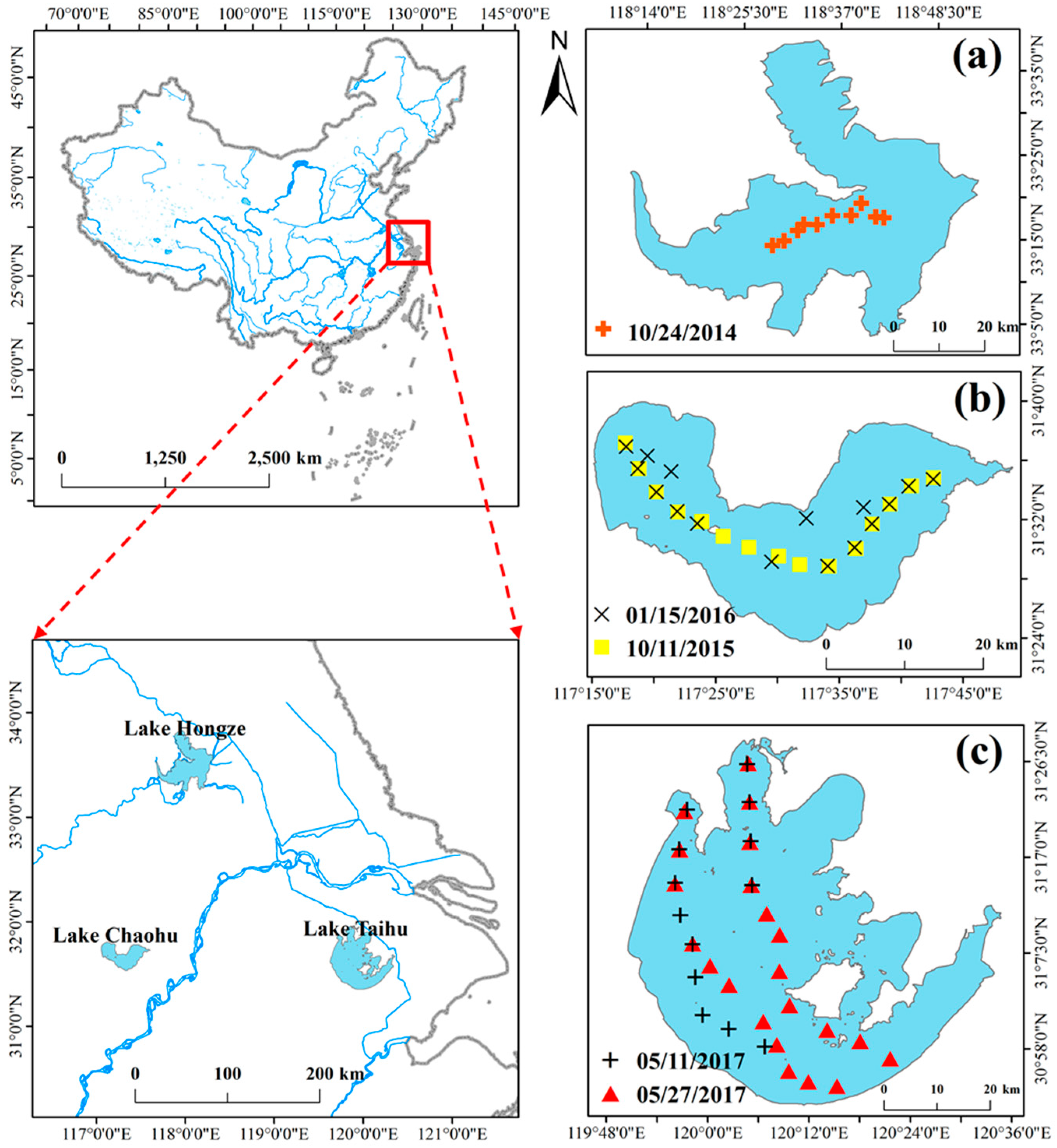
Lake Hongze (Figure 1a), Lake Chaohu (Figure 1b) and Lake Taihu (Figure 1c) are the fourth fifth, and third largest freshwater lake in China, with areas of ~1576.9 km2 (33°06′–33°40′N, 118°10′–118°52′E), 770 km2 (31°25′–31°43′N, 117°17′–117°51′E), and 2338 km2 (33°06′–33°40′N, 118°10′–118°52′E) respectively. The three lakes are shallow with an average water depth lower than 3 m, with high turbidity and with a eutrophic status. All provide important potable water sources to the local populations [28,29]. Lake Taihu and Lake Chaohu are characterized by extensive algal blooms [30]. Typically, their optical properties are dominated by phytoplankton, suspended matter, and CDOM (colored dissolved organic matter) [28]. These three lakes were selected because of their importance and complexity, to test the performance of AC algorithms over inland waters.
2.1.2. Field Measurements
Spectral data were measured by the spectrometer (ASD FieldSpec 4) following NASA Ocean optics protocols [31]. The total water-leaving radiance (Lt) ranges from 350 to 2500 nm, reflectance and radiance of reference panel (ρp, Lg, respectively), and sky radiance (Lsky) were measured via this instrument at 90° azimuth with respect to the sun and with a nadir viewing angle of 45° at each station. The water surface reflectance factor σ was assumed to be 0.028 [32] considering the wind speed (<5 m/s)and sky conditions (under clear sky or low cloud) of the field measurements. For each site, the remote sensing reflectance (Rrs) measurements were conducted 15 times to obtain the average value [33], from the ratio of water-leaving radiance (Lw) to incident downwelling plane irradiance (Ed):
The water samples were collected near water surface (<0.3 m), and were stored in the dark at 4 °C before laboratory analysis. According to NASA recommended protocols, concentration of chlorophyll-a (Chla) was measured spectrophotometrically using a Shimadzu UV-2600 spectrophotometer [34,35]. Concentrations of SPM (suspended particle matter) were determined gravimetrically in laboratory, and this matter was further differentiated into suspended particulate inorganic matter (SPIM) and suspended particulate organic matter (SPOM) by burning organic matter from the filters [36,37]. Spectral absorption coefficients of particulate involved phytoplankton (aph(λ)) were determined using the quantitative filter technique [38]. Spectral absorption coefficients of CDOM (ag(λ)) were determined using a Shimadzu UV-2600 spectrophotometer with Milli-Q water as the reference. Absorption coefficients of pure water (aw(λ)) were obtained from Pope and Fry (1997) [39]. Further details of the field measurements of bio-optical parameters and processing methods can be found in the previous studies [40,41].
2.1.3. Satellite Data and Data Matching
Five images of Level-1 from OLI sensor onboard the Landsat-8 (Table 2) were acquired from USGS (United State Geological Survey) (http://earthexplorer.usgs.gov/). The Level-1 data are provided in GeoTIFF format, with each spectral band in a separate file that has been mapped to a common UTM (Universal Transverse Mercator) projection, and the full suite of spectral band files are packaged into a compressed tape archive (tar) file that also includes a MTL (Landsat Metadata) file containing scene-specific time and location information [42]. These cloud free OLI images were processed to Rrs products via atmospheric correction, and then compared to in situ Rrs data. In order to minimize the effects of temporal and spatial mismatches between satellite and in situ data, the time window was narrowed to ~±3 h of the Landsat-8 overpass. For the sake of ensuring spatial data consistency, model-measured Rrs spectral data were derived by averaging a 3 × 3 pixel area surrounding the in situ data location.
2.2. Atmospheric Correction Algorithms
2.2.1. The Water-Atmospheric Correction Algorithms
Water-atmospheric correction algorithms on narrow band sensors were developed specifically for remote sensing of aquatic ecosystems [9,25,43]. In general, four water-ACs [6,7,24,25,26] are usually used, based on the assumptions that (1) pixels of water meet the requirements of “black pixel” assumption [4]; (2) the accuracy of aerosol model for extrapolation meets the real aerosol model [8]. It is worth considering their suitability for turbid waters. ACOLITE was developed for atmospheric correction for both OLI and MSI (MultiSpectral Imager) on Sentinel-2. The ACOLITE software (acolite_py_win_20180925.0) includes two atmospheric correction algorithms: EXP (exponential extrapolation) and DSF (dark spectrum fitting).
(1) SWIR
For turbid waters, the NIR black water assumption is often invalid because phytoplankton, detritus, and suspended sediment contribute to NIR backscatter [6,7]. SWIR bands have a higher absorption with respect to NIR bands [44]. The black pixel assumption is generally valid for SWIR bands at 1640 nm and 2130 nm, even for extremely turbid waters [45]. The SWIR algorithm process is the same as GW94, replacing the NIR bands with SWIR bands. Here, we use SeaDAS 7.4 [42] to process the satellite data via SWIR algorithm.
(2) EXP
The EXP algorithm is based upon exponential extrapolations of the ratio of multiply scattered SWIR aerosol reflectance in the visible bands. There is no use of aerosol LUTs (lookup tables). EXP reduces the noise from SWIR bands through spatial smoothing [25]. Two SWIR bands (1609 nm and 2201 nm) of OLI were used for aerosol determination in ACOLITE (v20180925).
(3) DSF
DSF was developed by Vanhellemont et al. [26] and integrated into a Python version of ACOLITE (acolite_py_win_20180925.0). The “dark pixels” for atmospheric correction in DSF are more flexible than in EXP and SWIR. In GW94, SWIR or EXP, dark targets pixels in NIR or SWIR are fixed while the band selection of “dark targets” is performed dynamically in the DSF algorithm. The darkest pixels in DSF are searched from all the image pixels. The aerosol optical thickness (AOD) is derived from the darkest pixels using a LUT, then used in the AC process. The DSF algorithm achieved satisfactory results on the Belgian coast.
(4) MUMM
The MUMM algorithm uses an alternative method to estimate the marine contribution in the NIR, as proposed by Ruddick et al. [6]. This algorithm replaces the assumption that the water-leaving radiance is zero in the NIR with the assumption of spatial homogeneity of the NIR band ratios for aerosol and water-leaving reflectance over the subscene of interest [6,46,47]. These assumptions are extended into the turbid waters, and the MUMM accuracy is highly dependent on the validity of the assumptions for a given image. The MUMM can be summarized as follows: (1) enter the atmospheric correction routine (i.e., GW94) to produce a scatter plot of the Rayleigh-corrected reflectance, ρrc(λ1) and ρrc(λ2), for the study region; (2) calculate the calibration parameter ε based on the scatter plot mentioned above; (3) reenter the atmospheric correction routine with data for the Rayleigh-corrected reflectance and use Equations (2) and (3) to determine ρa(λ1) and ρa(λ2), taking into account the nonzero water-leaving reflectance; (4) continue as in the standard GW94 algorithm [48].
where α is the ratio of the water-leaving radiance in NIR bands, ρa is the reflectance due to the aerosol scattering and the interaction between molecular and aerosol scattering reflectance; ρrc, is the top-of-atmosphere signal corrected for Rayleigh scattering, ε is the ratio of ρa. α is defined as ratio of the red band and NIR band; fixed for OLI to a value of 8.7 [49].
2.2.2. The Land-Atmospheric Correction Algorithms
Three popular atmospheric correction algorithms designed for land (land-AC) (FLAASH, 6SV, and QUAC) were assessed. FLAASH and 6SV are based on radiative transfer models and QUAC on a dark object assumption. Radiative transfer models consider the radiation transmission process in the range of visible light to the SWIR band. They describe the condition of the radiation source, the atmospheric status (including Rayleigh scattering, aerosol scattering, and vapor absorption), and the geometric conditions of the sensor. The key is to acquire in situ atmospheric parameter data simultaneously with satellite data acquisition. Actually, it is rarely possible to synchronously obtain such information. Therefore, standardized atmospheric parameters are used during the atmospheric correction. Dark targets or black pixels are usually used to derive the aerosol scattering [14,16,50,51]. AC algorithms for water strictly define black pixels, thus, dark objects required for land-AC are widely defined, including dense vegetation [52], water [53], and shadow waters [54]. The QUAC is typical of algorithms based on dark objects. The AC algorithm-driven surface reflectance is calculated as Rrs by dividing by π, because the water is approximated as a Lambert body [6,25,55,56,57].
(1) FLAASH
FLAASH was developed on the basis of the MODTRAN (MODerate resolution atmospheric TRANsmission) code by the Air Force Research Laboratory, Hanscom AFB, and Spectral Sciences, Inc. It has a unique solution to each image, because the atmospheric parameters are estimated from the characteristics of the atmosphere in image pixels, and atmospheric information is assessed by the dark target method based on the image itself [58]. Both the standard atmospheric model and aerosol model from MODTRAN are used to replace the real-time atmospheric parameters, which broaden the application of the FLAASH and improve its stability. The aerosol model for FLAASH is urban, due to the study areas are next to the cities, and the visibility value setting is the same as in Rotta et al. [59].
(2) 6SV
6SV is the vector version of 6S (Second Simulation of the Satellite Signal in the Solar Spectrum) [60,61], a basic radiative transfer code used to calculate lookup tables in the atmospheric correction algorithm (http://6s.ltdri.org). It enables accurate simulations of satellite and plane observations, accounting for elevated targets, the use of anisotropic and Lambertian surfaces, and the calculation of gaseous absorption. The code is based on the method of successive orders of scattering approximations [15]. For detailed corrections, 6SV, the latest code for atmospheric correction requires ancillary data such as water content, ozone content, and aerosol optical depth, as well as terrain elevation [62]. Standard atmospheric model and aerosol model from the 6SV algorithm were used in the present study due to the lack of real-time atmospheric data. The observed geometry is obtained from MTL text, and other settings are same as Shen et al (2018) [63].
(3) QUAC
QUAC (Quick Atmospheric Correction) is an algorithm based on dark targets. Three assumptions are considered: (1) the image must present more than 10 spectrally different pixels; (2) the standard deviation of the reflectance from end-member pixels is spectrally independent and can be used to calculate the transmittance; and (3) there is a relevant number of dark pixels to calculate an invariant baseline, assumed as a measurement of attenuation (scattering and absorption) and the adjacency effect [17]. The computational speed of the atmospheric correction method is significantly faster than radiative transfer model based methods because QUAC does not involve first principles radiative-transfer calculations, and only requires an approximate specification of sensor band locations (i.e., central wavelengths) and their radiometric calibration [53].
2.3. Water Type Classification
Normalized through depth at 675 nm (NTD675) [64] was used for classification of inland water studied:
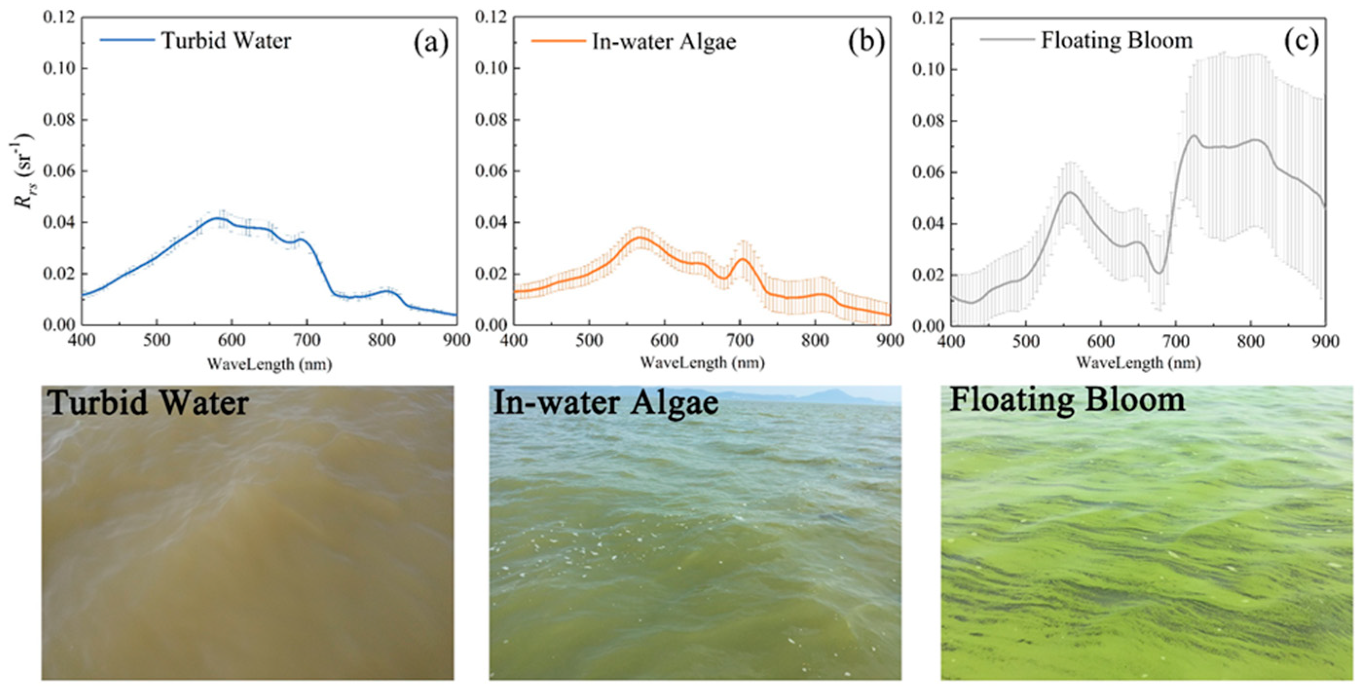
where nRrs(λ) referred to the normalized remote sensing reflectance at wavelength λ nm by using reflectance at 675 nm. In our study, waters were classified into three types: turbid water (TW), in-water algae (IW), and floating bloom (FB) [64].
2.4. Statistical Indices
To evaluate performance of the algorithm, the determined coefficient (R2), the root-mean-square-error (RMSE), the mean absolute percentage error (MAPE), and bias were used:
where Rirs is the in situ data, Rmrs is the OLI data after atmospheric correction, and n is the number of match-ups.
3. Results
3.1. Spectrums and Water Conditions of Study Areas
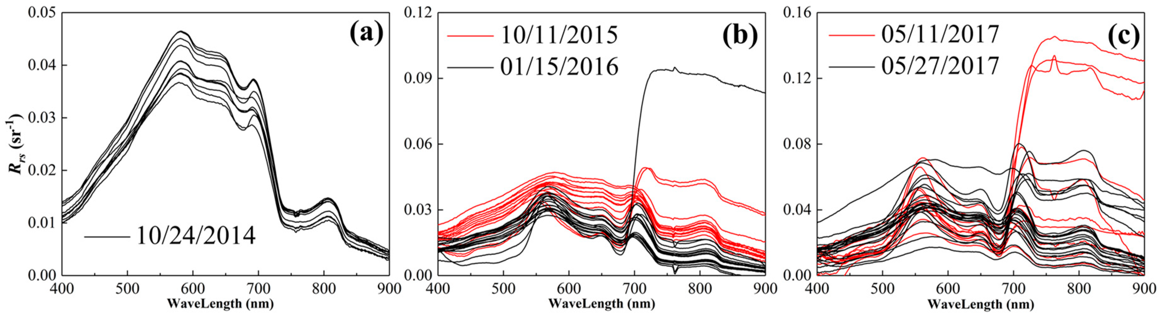
The measured Rrs within the range of 400–900 nm, associated with 74 sites over three lakes (Figure 1), are shown in Figure 2a (Lake Hongze), 2b (Lake Chaohu), and 2c (Lake Taihu). The spectral shape of Lake Hongze on 24 October 2014 (Figure 2a) was monotonous, with a flat spectrum at 550–650 nm, and the Rrs are characteristic of highly turbid waters and are similar in shape to previously reported spectra [65,66]. The Figure 2b,c showed that the spectral characteristic of Lake Chaohu and Lake Taihu are complex. In Lake Chaohu and Lake Taihu, the spectral characteristics of turbid waters were found, furthermore, other spectra also showed distinct increased water-leaving radiance within NIR region, i.e., 700 to 900nm. The higher variability in the spectral curves in Figure 2b,c within the 700–900 nm range reflects a larger variability in optically active constituents of lake waters in Lake Chaohu and Lake Taihu than in Lake Hongze.
Table 3 shows the variations of bio-optical properties of three lakes (Lake Hongze, Lake Chaohu, and Lake Taihu). For the waters of Lake Taihu, Chla showed highest variability from 19.96 to 1022.53 μg/L (206.13 ± 267.93 μg/L), SPOM also showed highest variability from 4.00 to 321.33 mg/L (72.04 ± 85.48 mg/L). Correspondingly, the ag(440) and aph(665) of Lake Taihu covered wide ranges. While the variation ranges of bio-optical properties of Lake Hongze was much narrower than that of Lake Chaohu and Lake Taihu (Table 3), especially ag(440) (1.38 ± 0.13) and aph(665) (0.19 ± 0.03). On the other hand, the mean SPOM/SPIM value of Lake Hongze was 0.25, Lake Hongze was dominated by SPIM, while the mean SPOM/SPIM values of Lake Chaohu and Lake Taihu were more than 1.39, and these two lakes were dominated by SPOM.
3.2. Water Optical Properties and the Classification
For turbid water, there were three peaks at around 550, 710, and 810 nm, and the Rrs slowly decreased from 550 to 710 nm (Figure 3a). The spectral peaks of in-water algae were salient at around 550 and 710 nm and, from 710 to 900 nm, the spectrum shown a downward trend (Figure 3b). For the floating bloom waters, however, the Rrs in the NIR region was normally higher than that at around 680 nm with a spectral shape similar to that of vegetation (Figure 3c). These spectral characteristics of water reflectance were important in atmospheric correction algorithms, especially for the “black pixel” assumption. The average biochemical parameters for each water type show clear differences (Table 4). The Chla, SPOM, SPOM/SPIM (ratio of SPOM to SPIM), and aph(665) generally showed an increasing trend from turbid water to in-water algae and floating bloom. The Chla values indicated that three water types are eutrophic. Floating bloom had obvious high value of Chla (198.04 ± 203.85 μg/L) and relatively higher SPOM (117.27 ± 69.46 mg/L) and aph(665) (6.59 ± 8.07) than other water types. The mean SPOM/SPIM value was 0.28 in turbid water, meaning that turbid water was dominated by SPIM. However, the mean SPOM/SPIM values were more than 1.5 in in-water algae and floating bloom, revealing that the two water types are dominated by SPOM. Actually, the SPOM in in-water algae and floating bloom was mainly phytoplankton. According to field observations, in-water algae is dominated by algae phytoplankton accumulation in the water column, and floating bloom waters are dominated by floating phytoplankton.
3.3. Assessment of the Water-AC Algorithms
3.3.1. Comparison with In Situ Measurements
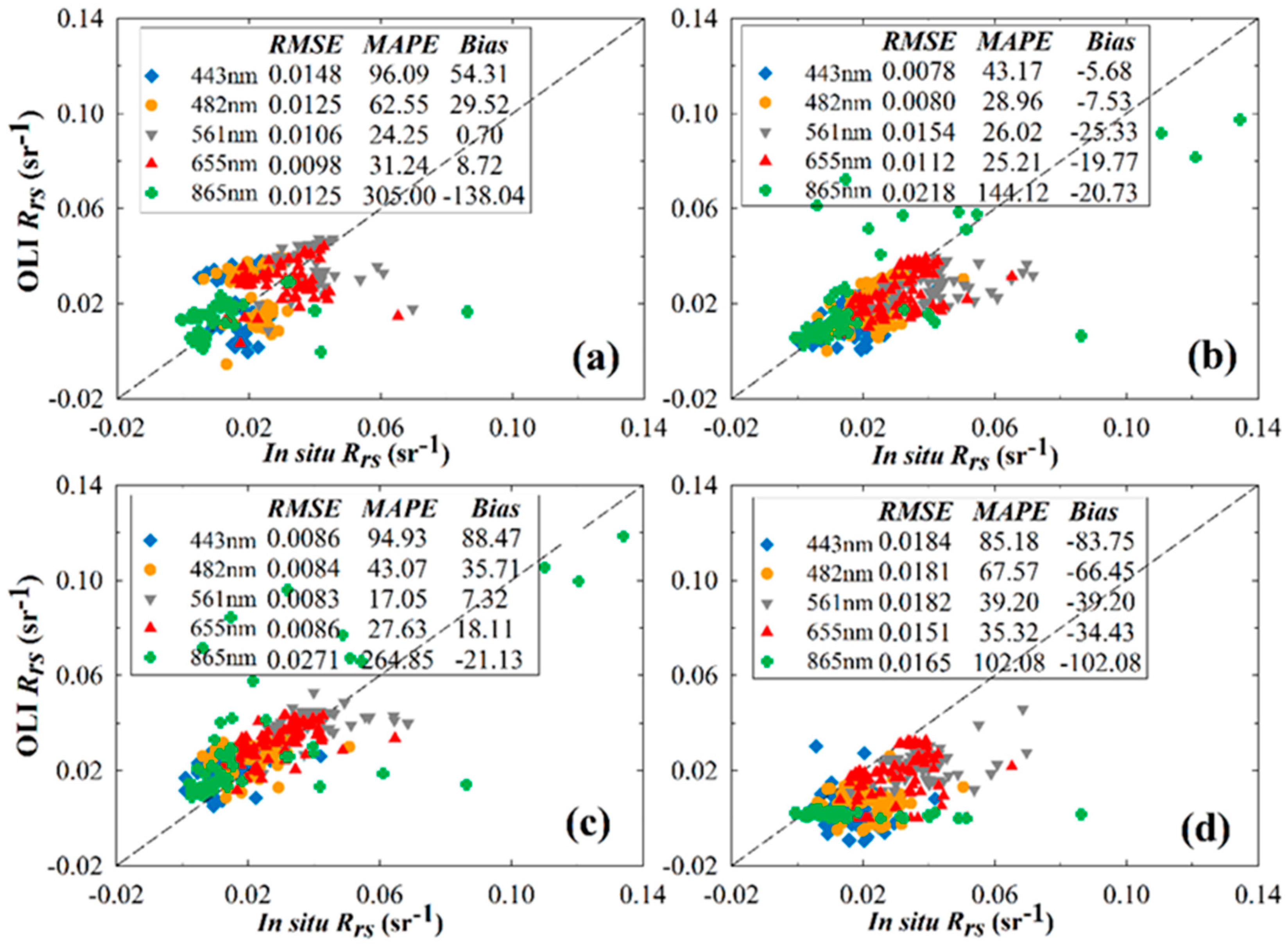
In this section, the performances of water-atmospheric correction algorithms will be assessed using in situ data. It needs to be pointed out that only 56 match-up sample points of in situ data were used for the evaluations of SWIR and MUMM algorithms because of water pixel mask derived by AC algorithms. The DSF algorithm provided the smallest RMSE and MAPE at 561 nm (RMSE ~ 0.0083 sr−1; MAPE ~ 17.06%) and 655 nm (RMSE ~ 0.0086 sr−1; MAPE ~ 27.63%) (Figure 4c). The DSF and SWIR algorithm showed quite similar MAPE values at 443, 482, 655, and 865 nm bands (Figure 4a,c). The EXP algorithm derived the smallest RMSE and MAPE of Rrs(443) (RMSE ~ 0.0078 sr−1; MAPE ~ 43.17%) and Rrs(482) (RMSE ~ 0.0080 sr−1; MAPE ~ 28.96%), but the data plots at 865 nm were discrete in the measured high value (Figure 4b). Plots derived by the MUMM algorithm were generally under the 1:1 line (Figure 4d) and the Rrs(443) retrieved by MUMM were negative. Compared to the accuracy of the SWIR, EXP, and DSF algorithms, MUMM was low (RMSE > 0.0151 sr−1; MAPE > 39.20%). Furthermore, all four water-AC algorithms failed at 865nm band (RMSE > 0.0125 sr−1; MAPE > 102.08%).
3.3.2. Band Ratios
Band ratio algorithms are commonly used in retrieval of water biogeochemical products, and can reduce the systematic retrieval error caused by atmospheric corrections. They can be used to test the ability of AC methods to accurately retrieve the spectral shape of Rrs at the water surface from TOA radiance. According to the definition of α, the ratio of band 3 and band 4 for the OLI sensor is fixed at a value of 8.7 [49]. The Rrs(865)/Rrs(655) retrieved by MUMM was not discussed.The lowest values of three statistical indices (Table 5) was in Rrs(655)/Rrs(561), and the highest values were in Rrs(865)/Rrs(561) and Rrs(865)/Rrs(655). The Rrs(655)/Rrs(561) had the best agreement with in situ data, the best algorithm was SWIR algorithm, and the worst was MUMM algorithm. Rrs(655)/Rrs(561) had a similar accuracy of RMSE ~0.01 and MAPE ~11% across algorithms (Table 4). Remarkably, four water-AC algorithms all failed in the band ratios with the NIR band (Rrs(865)/Rrs(561) and Rrs(865)/Rrs(655)), and the RMSE and MAPE values of band ratios with the NIR band were more than 0.3916 and 89.43%, respectively. Similarly, the RMSE and MAPE values of the band ratios with 443 nm band were more than 0.1758 and 46.11%, respectively. The large error in band ratios with NIR band or with 443 nm band may reduce the robustness of the retrieval methods of water biogeochemical products. While Rrs(655)/Rrs(561) was supported by four water-AC algorithms, Rrs(655)/Rrs(561) may reduce the uncertainty of the inversion algorithms brought by the AC algorithm. Accordingly, EXP achieved the best accuracy in band ratios (except the band ratios with NIR band), while MUMM was the worst performer of the four water-AC algorithms.
In summary, the MUMM algorithm with fixed α of 8.7 did not work in our study areas, and the SWIR algorithm did not meet the requirements [2]. The accuracy of EXP was very similar to that of DSF.
3.4. Assessment of the Land-AC Algorithms
3.4.1. Comparison with In Situ Measurements
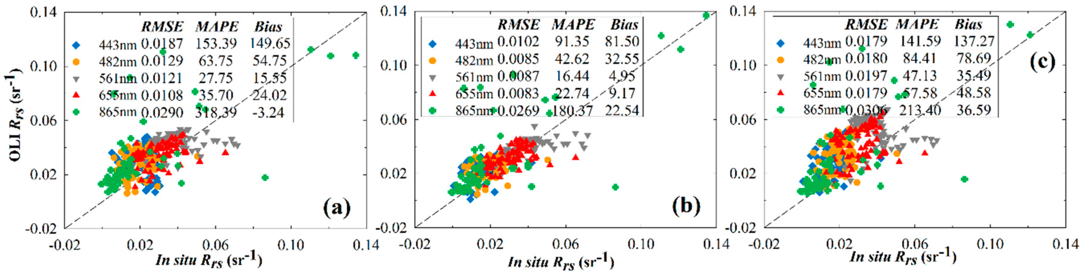
The land-AC algorithms failed at 443 nm (RMSE > 0.0102 sr−1, MAPE > 91.35%) and 865 nm (RMSE > 0.0269 sr−1, MAPE > 180.37%), which was similar to the results of water-AC algorithms. Comparatively, the accuracy of land-AC algorithms at 561 nm was the best. The EXP and MUMM algorithms underestimated the water-leaving reflectance the water-leaving reflectance (Figure 4b,d). However, the land-AC algorithms overestimated the water-leaving reflectance (Figure 5). The MAPE of FLAASH-derived Rrs was larger than 27.75%, and the RMSE of that was more than 0.0108 sr−1 (Figure 5a). The RMSE and MAPE of QUAC-derived Rrs was larger than 0.0179 sr−1 and 47.13%, respectively (Figure 5c). Compared with FLAASH and QUAC, the 6SV algorithm produced the smallest overall RMSE and MAPE (Figure 5b). The MAPE of 6SV-derived Rrs(561) and Rrs(655) were 16.44% and 22.74%, which met the requirement for Case II remote sensing retrieval at 561 nm and 655 nm [2]. However, 6SV did not work at the blue band (443 nm) and NIR band (865 nm).
3.4.2. Band Ratios
Rrs(655)/Rrs(561) retrieved by land-AC algorithms provided the highest accuracy of all band ratios (RMSE < 0.0963, MAPE < 11.50%) (Table 6), while the accuracy of the retrieved band ratios with the NIR band was the lowest (RMSE > 0.6360, MAPE > 149.59%). This was similar to the performances of water-AC algorithms. Different from the large gap between the performance of the water-AC algorithms in band ratios, the three land-AC algorithms showed similar accuracy for Rrs(482)/Rrs(561), Rrs(655)/Rrs(561), and Rrs(482)/Rrs(655). Notably, the QUAC algorithm in the band ratios was improved (Table 5) and could accurately retrieve the spectrum shape. 6SV had better performance than other algorithms, however, the advantage of 6SV were not significant.
3.5. EXP vs. 6SV
Three water-AC algorithms (SWIR, EXP, DSF, and MUMM) and three land-AC algorithms (FLAASH, 6SV, and QUAC) were evaluated in the previous sections, and EXP and 6SV were, respectively, the optimal algorithms.
3.5.1. Intercomparison of AC Algorithms
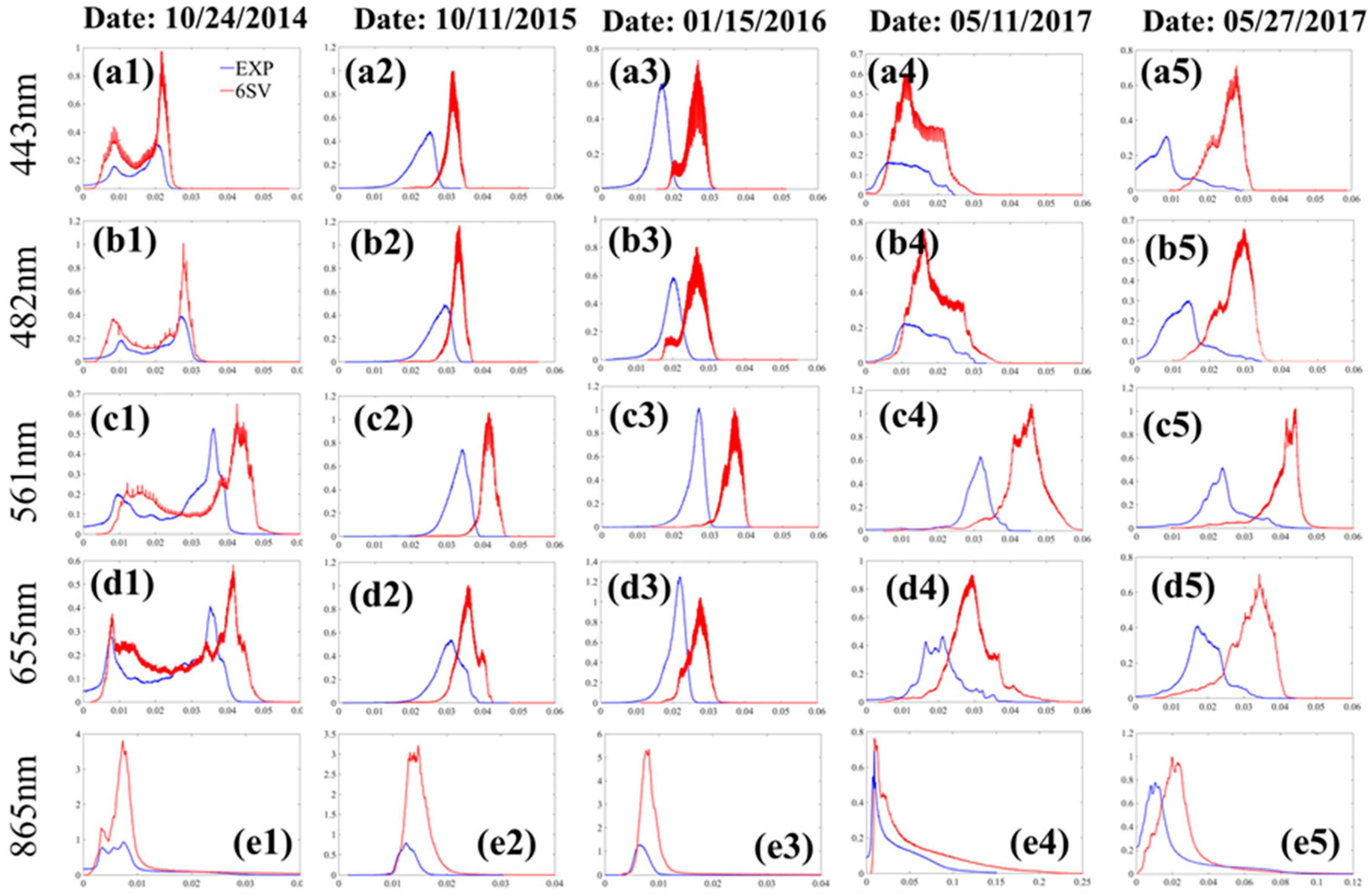
As Figure 6 shows, the 6SV-driven red lines were generally to the left of the EXP-driven blue lines. This means that Rrs(λ) derived by the 6SV algorithm were larger than those derived by the EXP algorithm (Figure 7), especially at 561 nm, and the difference between the two AC algorithms was more obvious. Compared with in situ data, 6SV overestimated water-leaving reflectance in all bands (Figure 5b) whereas EXP underestimated it (Figure 4b). The errors of Rrs(561) and Rrs(655) retrieved by 6SV were less than that retrieved by EXP, and it met the inversion requirements of remote sensing of Case II waters [2], yet both EXP and 6SV failed at 443 and 865 nm. The accuracy of EXP and 6SV were satisfactory in TW waters, and EXP was better than 6SV. Although the accuracy of 6SV met the requirements of remote sensing inversion in 561 and 655 nm of IW waters, both EXP and 6SV failed in FB waters. For the band ratios, the accuracy difference between 6SV and EXP was small. This feature was same in the three water types. The errors of the 443 nm band ratios retrieved by 6SV were larger than that retrieved by EXP, but the performance of 6SV was better than that of EXP for the 865 nm band ratios.
Based on this analysis, the accuracies obtained by EXP and 6SV were similar. The differences in the accuracy of EXP and 6SV varied in different water types: EXP had a significant advantage in turbid waters and 6SV was more accurate in in-algae waters, but both failed in floating bloom waters.
3.5.2. Performance of EXP and 6SV in SPM Estimation
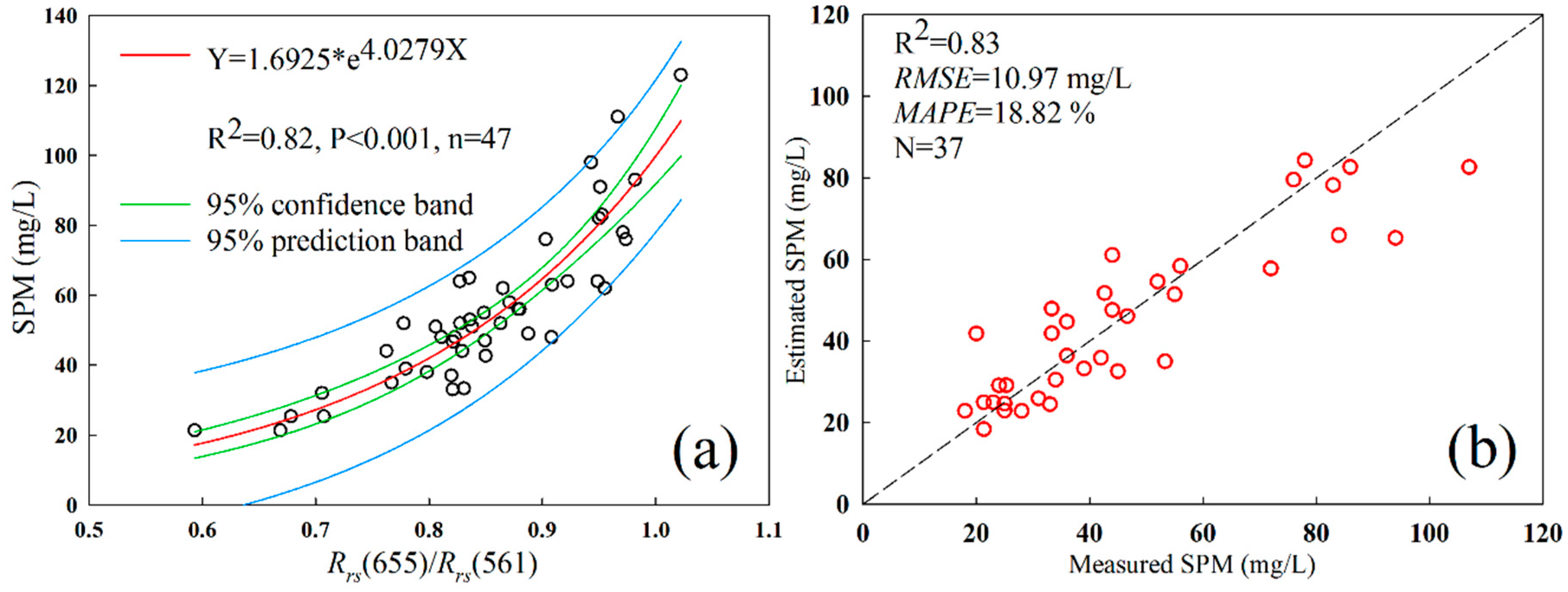
To understand the performance of EXP and 6SV in remote sensing retrieval of ocean (water) color, a retrieval model for SPM (suspended particle matter) in Lake Chaohu was developed using in situ data. The SPM data of Chaohu came from four field sampling data time points (the dates were 09/11/2016, 12/07/2016, 04/27/2017, and 08/22/2017) with a total of 84 samples, of which 47 samples were used to develop the SPM model and 37 samples were used to validate the SPM model. It should be pointed out that these in situ sampling data are not the synchronization data of OLI, only used for the development and verification of SPM model. It was used to evaluate the effects of the EXP and 6SV algorithms on the accuracy of the retrieval model for SPM. Since the reflective signals of the water column were weak or even absent in algae bloom waters, the in situ data of algae blooms were eliminated in this section. Based on the results for the in situ-measured Rrs(λ) and in situ measurements of SPM, the empirical band ratio algorithm with the highest coefficient of determination was obtained through regression analyses among different band combinations that estimate SPM, as follows:
The coefficient of determination, R2, for the best regression relationship of the logarithmic function between the simulated in situ-measured Rrs(655)/Rrs(561) and in situ SPM data was 0.82 (P < 0.001) (Figure 8a). The proposed model performed well for the validation dataset (Figure 8b). The MAPE of the SPM model for the in situ dataset was 18.82% and RMSE was 10.97 mg/L. Comparisons between the in situ measurements and the derived SPM data were evenly distributed along the 1:1 line. These results indicated that the proposed model could be used to estimate SPM with satisfactory performance in these inland waters.
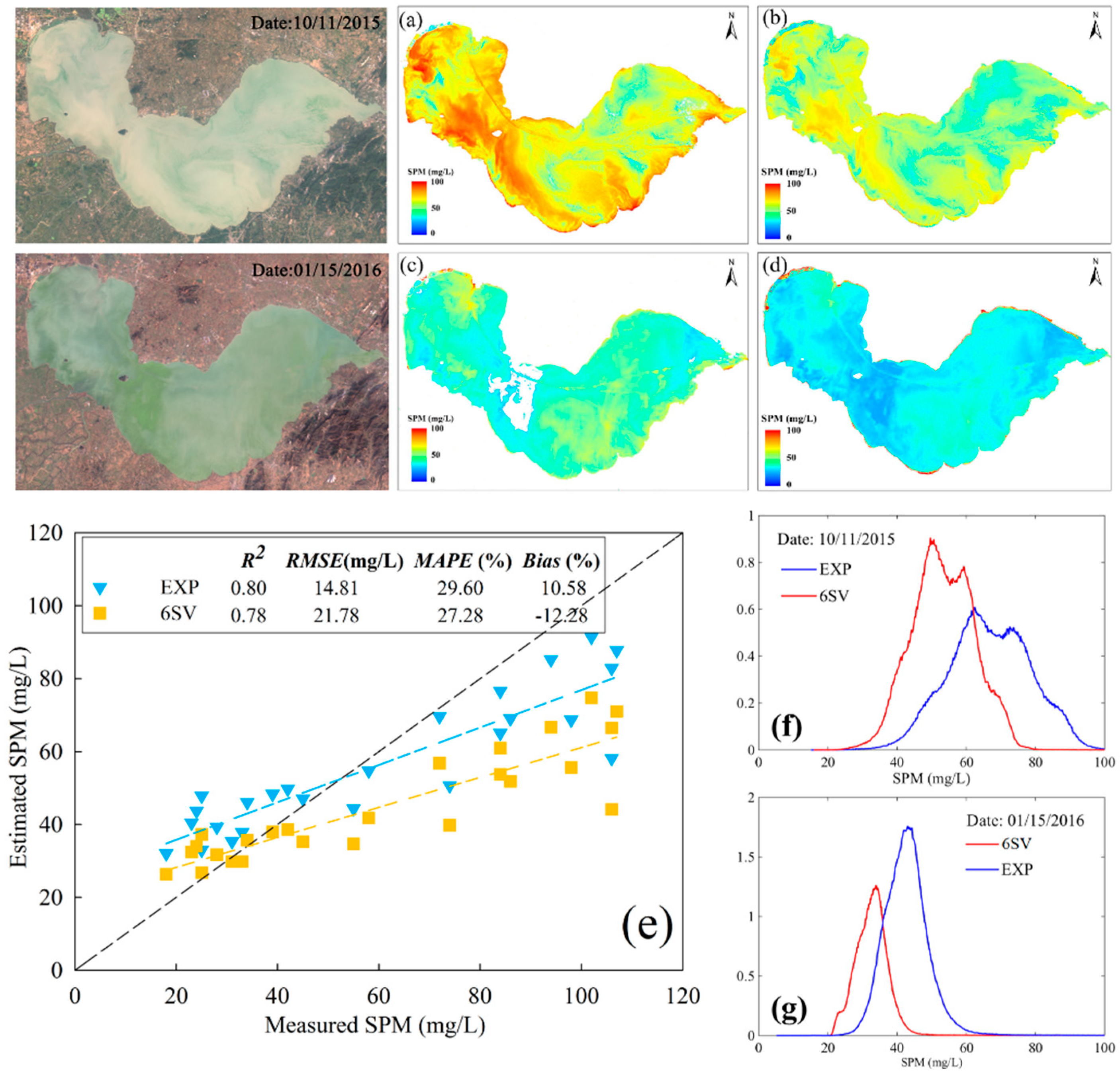
The spatial distributions of the EXP-derived and the 6SV-derived SPM were consistent, and the absolute SPM values derived by EXP and 6SV were comparable (Figure 9a–d): the EXP-retrieved SPM was 12 to 100 mg/L and the 6SV-retrieved SPM was 2 to 82 mg/L. Furthermore, the spatial distribution of low SPM values matched the distribution of algae blooms, as the absorption peak of chlorophyll-a near 665 nm reduced the Rrs(655)/Rrs(561). As shown in Figure 9f,g, the SPM values derived by EXP were higher than those by 6SV algorithm. The R2 of the regression relationship between the simulated in situ-measured SPM and OLI-estimated SPM derived by EXP and 6SV were 0.80 and 0.78, respectively (Figure 9e). Based on the statistical indices, the estimation accuracy of the EXP-derived SPM was higher than that of the EXP-derived SPM, however, the fitting lines of the scatter points were almost parallel. On the left side (Figure 9e) of the measured SPM (<50 mg/L), the EXP-derived and 6SV-derived SPM were overestimated, and the scatter points of the 6SV-derived SPM were closer to the 1:1 line (dashed dark line) than the EXP-derived SPM. However, on the right side of the measured SPM (>50 mg/L), the estimated SPM was less than the measured SPM and the scatter points of the EXP-derived SPM were closer to the 1:1 line.
4. Discussion
4.1. Assessment of AC Algorithms for Different Water Types
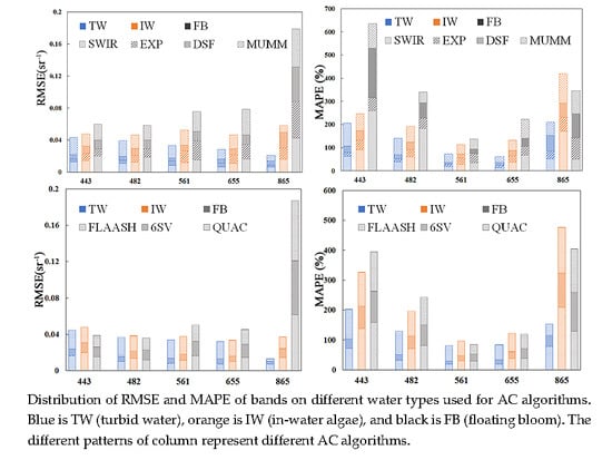
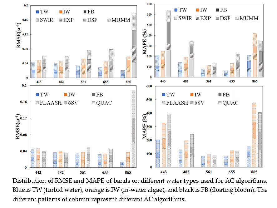
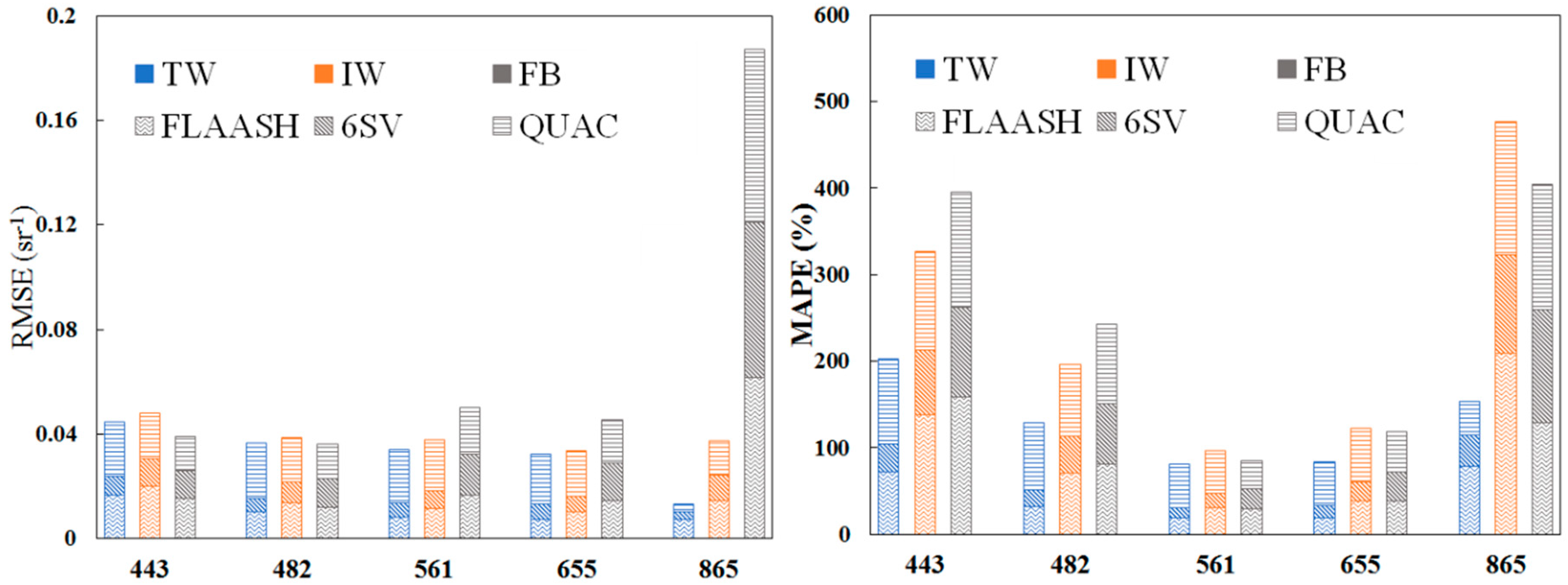
Chlorophyll and SPM contents of all three water types increased in turn (Table 4). As shown in Figure 10, the performance of water-AC algorithms in TW were better than those in IW and FB. Since the DSF-derived Rrs(561) obtained the best accuracy, this was used as an example: the RMSE of the DSF-derived Rrs(561) for turbid, in-water algae, and floating bloom waters was 0.0038, 0.0071, and 0.0120 sr−1, respectively; the MAPE of that was 7.62%, 16.80%, and 20.59%, respectively (Figure 10). For land-AC algorithms (Figure 11), the 6SV-derived Rrs(561) was taken as an example: the RMSE of the 6SV-derived Rrs(561) for turbid, in-water algae, and floating bloom waters was 0.0053, 0.0070, and 0.0157 sr−1, respectively; the MAPE was 11.14%, 16.57% and 23.17%, respectively. The performances of the AC algorithms in turbid waters were acceptable, however, the errors from estimation of AC algorithms in in-water algae and floating bloom waters reduces the overall accuracy of algorithms. The performance of the AC algorithms was poor for high chlorophyll and high SPM concentration waters. Further analysis was necessary to understand why the AC algorithms failed in our study area.
The QUAC algorithm is based on dark targets and relies on three assumptions [17]. In practice, the lowest-value set of pixels in the image is selected as the dark pixels, but the water pixels are often the lowest-value pixels in the image. Therefore, the water pixels are often used as a dark target for QUAC algorithm. As a result, the performance of the QUAC algorithm for water inevitably deteriorates and the accuracy decreases. Although the FLAASH atmospheric correction algorithm is based on the radiation transmission model, FLAASH uses the same dark-target method as QUAC to estimate aerosol scattering for the sake of algorithm versatility [67]. This is different from 6SV, which relies on the radiative transfer model to solve aerosol scattering. In the 6SV algorithm, the input parameters are the key to the accuracy of the algorithm and the aerosol model is critical for estimation of the aerosol scattering. The SWIR, EXP, DSF, and MUMM algorithms are based on the “black pixel” assumption and the comparison with the real situation at the time of satellite passing.
4.2. Does It Fit the “Black Pixel” Assumption?
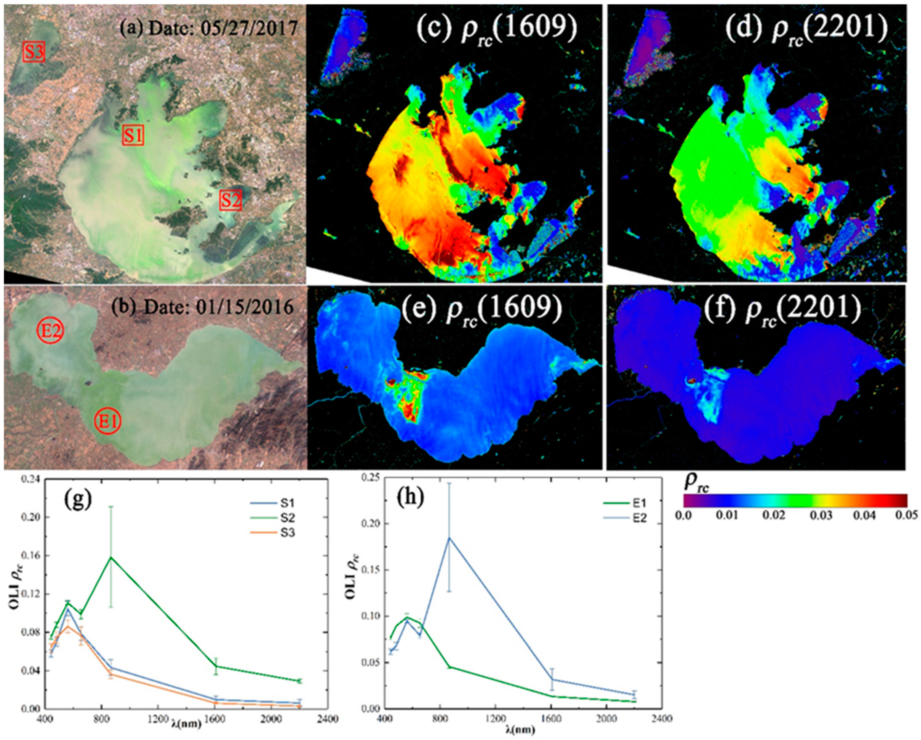
The Rayleigh-corrected reflectance data (ρrc(λ), derived by SeaDAS 7.4) for Lake Taihu (date: 05/27/2017) and Lake Chaohu (date: 01/15/2016) were taken as examples to assess the “black pixels” of inland waters in the NIR and SWIR bands. The two OLI images showed algal blooms in Lake Taihu and Lake Chaohu (Figure 12a,b). The average ρrc from five 100-by-100-pixel boxes (and circles), extracted from the 05/27/2017 and 01/15/2016 images, range from turbid (S1, S3, and E1) to floating bloom waters (S2, E2).
As shown in Figure 12g–h, the ρrc (SWIR) extracted from S2 and E2 were higher than those from S1, S3, and E1, and the distribution of high value pixels of the Rayleigh-corrected reflectance was the same as the distribution of floating bloom waters (Figure 12c–f). This indicated that the high contributions at 1609 nm and 2201 nm were from floating-bloom waters, and not from the atmosphere. When blooms occurred, the water-leaving reflectance of floating bloom waters in SWIR bands was strong and no longer met the “black pixel” assumption. Thus, the AC algorithms based on the black pixel assumption failed in floating bloom and in-algae waters. Although the “dark pixels” defined by DSF are dynamically selected, the SWIR bands of water were very important sources of dark pixels. Thus, the nonzero reflection in SWIR bands also affected the performance of the DSF algorithm.
From Equations (2) and (3), the α of the MUMM algorithm is the core correction parameter, and its value directly affects the accuracy of the algorithm. The MUMM algorithm uses the Red and NIR bands to extrapolate from NIR to visible bands, and fixes α as 8.7 for OLI [49]. Using in situ data, the mean α (red band/NIR band for OLI) was 2.5 and its SD (standard deviation) was 1.9. The absorption and reflectance of water in the NIR bands are not dominated by pure water when the water is very turbid or algal blooms occur, and the ratio of the water-leaving reflectance is not constant in the NIR bands [46]. This indicated why the MUMM algorithm failed in the study areas.
4.3. Does the Aerosol Model Accord with the Real Situation?
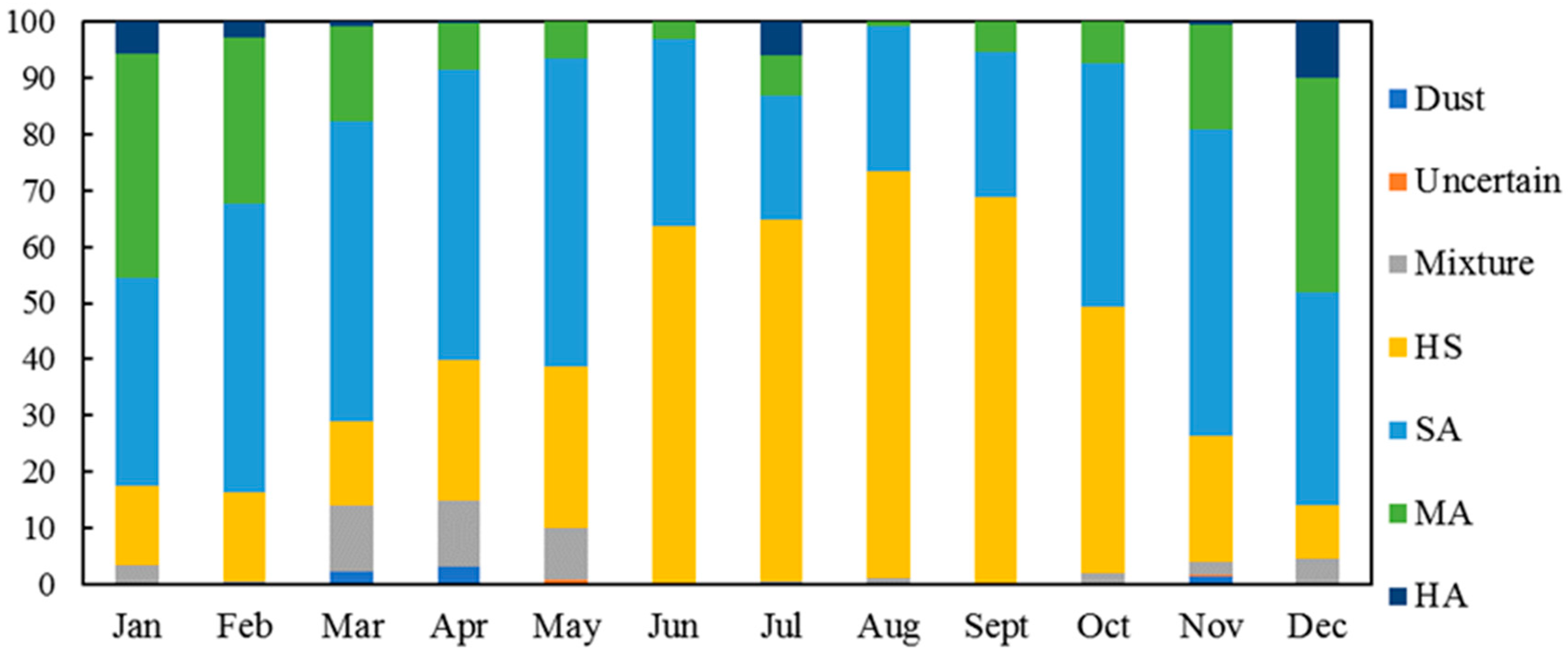
The aerosol model is another factor affecting the performance of the SWIR, DSF, and MUMM algorithms. AERONET Level 2 data (https://aeronet.gsfc.nasa.gov) from the Taihu station (2005–2018) were used for classification of aerosol types according to Lee’s classification method [68]. Lee’s method differentiates aerosol into 7 types: dust, uncertain, mixture, and highly absorbing (HA), moderately absorbing (MA), slightly absorbing (SA), and highly scattering (HS) fine-mode aerosols. The results of the aerosol type frequencies showed that the fine mode dominated the aerosol types of Taihu, primarily SA (43.96%) and HS (31.60%). This is a typical of urban or industrial aerosol sources. Figure 13 showed the frequency of seasonal variation of aerosol types from the Taihu AERONET station (from 2005 to 2018). HS dominated in the summer and fine mode aerosol type was dominant in other seasons. However, most aerosol models used by AC algorithms are non- and weakly absorbing aerosol types [3,8,26,69]. The absorption capacity of absorbing aerosol reduces the surface reflectance signal that the satellite sensor can receive, and the surface reflectance signal is overcome by a larger atmospheric signal than for non- and weakly absorbing aerosol types. However, due to the complexity of aerosol sources and types, it is difficult to develop aerosol models of dust atmosphere. This error cannot be avoided for atmospheric correction algorithms that rely on extrapolation of aerosol models. EXP is based upon exponential extrapolations of the ratio of multiply scattered SWIR aerosol reflectance into the visible bands, and aerosol LUTs (lookup tables) are not used in the EXP algorithm [25]. EXP avoids systematic errors caused by inaccurate descriptions of aerosol models. However, the EXP errors are larger in the blue bands due to the simple exponential extrapolation from NIR or SWIR bands.
4.4. Validation of EXP Algorithm
The EXP algorithm showed the best performance in our study areas, but how did the EXP algorithm perform in other areas? Caballero et al. [70] studied the TSS (Total Suspended Solid) levels for each dredging in Guadalquivir River (located in the southwest of the Iberian Peninsula and corresponds to one of the largest rivers in Spain) using EXP-driven images, and the employment of EXP algorithm seemed to properly correct atmospheric features of the OLI bands over the Guadalquivir region, yielding a reasonable spectral signature compared with the spectral signal of the visible and NIR bands driven by EXP algorithm, which revealed varying TSS concentrations as well. EXP has proven to be a very accurate scheme in the processing of medium-resolution images for the coastal waters of the Guadalquivir estuary [70]. Similarly, the performance of the EXP algorithm was accepted in Jiujing River (located in Xiamen city, China) [71]. Furthermore, Novoa et al. [72] compared the performances of EXP and MACCS (Multisensor Atmospheric Correction and Cloud Screening processor) in coastal waters. Both AC algorithms achieved good accuracy in coastal waters. However, the MACCS algorithm is based on land pixels and estimates the aerosol optical thickness combining a multispectral assumption. This method is not able to estimate the aerosol model and uses a constant model for a given site, which is a disadvantage for regions where the aerosol model is subject to large spatial variations [72]. This is also the disadvantage of AC algorithms that require pre-set aerosol model, such as 6SV. EXP uses an ocean color approach, and is considered more appropriate for the coastal waters of the study regions. Wei et al. [57] found EXP-derived Rrs had comparable spectral shape and magnitude to the corresponding in situ Rrs in the three regions with different CDOM (Colored Dissolved Organic Matter) levels, and the EXP worked better in inner bay and rivers, while it worked worse in coastal waters which had high bottom reflectance [73]. This was consistent with the verification results of Wei at al. [57] in optically shallow coral reef environment. The performance of the EXP algorithm was worse than GW94 algorithm in optical shallow waters [57]. The bottom reflectance contributed in SWIR bands may affect the atmospheric correction.
Overall, the assessment results showed the EXP algorithm can be effectively applied in turbid waters (including inland waters and coastal waters), but EXP did not work well in clear waters, algae blooms waters, or waters with bottom reflectance.
5. Conclusions
The present study compared four water-AC algorithms (SWIR, EXP, DSF, and MUMM) and three land-AC algorithms (FLAASH, 6SV, and QUAC) for inland waters using in situ data from shipborne measurements. The accuracy of EXP, DSF, and 6SV were similar, and their performance was better than the others. However, they all failed in the NIR band due to the effects of floating algae.
EXP, DSF, and 6SV achieved satisfactory accuracy in all bands for turbid waters but did not work in in-algae and floating bloom waters. This was associated with the high signals in these waters at the 1609 nm band of the OLI sensor, which was not in line with the “black pixel” assumption. SWIR bands in turbid water sites conformed to the “black pixel” requirement using in the SWIR, EXP, and DSF algorithms.
The aerosol type in the study area was dominated by absorbing fine-mode aerosols. However, most of the aerosol models used by the AC algorithms are non- and weakly absorbing aerosol types; thus, the inaccurate aerosol model limited the performance of the AC algorithms. The red–green ratio (Rrs(655)/Rrs(561)) was supported by all algorithms, and the empirical model based on the red–green ratio was successful in the SPM inversion of Lake Chaohu. The systematic retrieval error caused by atmospheric correction can be reduced by band ratio. Notably, all AC algorithms failed in retrieval of the band ratios formed by the NIR band. The present study shows that the EXP algorithm is suitable for turbid inland waters and achieving an elevated accuracy across inland waters with a range of trophic and optical conditions remains a challenge.
Author Contributions
D.W. and R.M. principally conceived of the idea for the study. D.W. was responsible for setting up the experiments, completing the experiments, wrote the paper and analyzed the data. R.M., K.X. and Steven Arthur Loiselle contributed to the analysis and discussion. All authors contributed to the writing of the manuscript.
Funding
This project was jointly funded by State Key Program of National Natural Science of China [No. 41431176], the National Natural Science Foundation of China [No. 41771366 & 41701416] and the key project of Nanjing Institute of Geography and Limnology [No. NIGLAS2017GH03].
Acknowledgments
The authors would like to thank the USGS for providing the Landsat-8 OLI data; NASA for providing the SeaDAS; Vanhellemont, Q. for providing the ACOLITE software; AERONET for providing the aerosol data; Jing Li, Zhigang Cao, Ming Shen and Junfeng Xiong, Tianci Qi, Xu Fang for their hard work. We also thank for the data support from “Lake-Watershed Science Data Center, National Earth System Science Data Sharing Infrastructure, National Science & Technology Infrastructure of China (http://lake.geodata.cn) and the ESA/MOST Dragon 4 program for facilitating this collaboration.
Conflicts of Interest
The authors declare no conflict of interest.
References
- Gordon, H.R. A Preliminary Assessment of the Nimbus-7 CZCS Atmospheric Correction Algorithm in a Horizontally Inhomogeneous Atmosphere. In Oceanography from Space; Gower, J.F.R., Ed.; Plenum Press: New York, NY, USA; London, UK, 1981; pp. 257–258. [Google Scholar]
- Wang, M. Atmospheric Correction for Remotely-Sensed OceanColour Products; International Ocean-Colour Coordinating Group: Monterey, CA, USA, 2010. [Google Scholar]
- Gordon, H.R.; Wang, M. Retrieval of water-leaving radiance and aerosol optical thickness over the oceans with SeaWiFS: A preliminary algorithm. Appl. Opt. 1994, 33, 443–452. [Google Scholar] [CrossRef] [PubMed]
- Siegel, D.A.; Wang, M.; Maritorena, S.; Robinson, W. Atmospheric correction of satellite ocean color imagery: The black pixel assumption. Appl. Opt. 2000, 39, 3582–3591. [Google Scholar] [CrossRef] [PubMed]
- Hu, C.; Carder, K.L.; Muller-Karger, F.E. Atmospheric Correction of SeaWiFS Imagery over Turbid Coastal Waters. Remote Sens. Environ. 2000, 74, 195–206. [Google Scholar] [CrossRef]
- Ruddick, K.G.; Ovidio, F.; Rijkeboer, M. Atmospheric correction of SeaWiFS imagery for turbid coastal and inland waters. Appl. Opt. 2000, 39, 897–912. [Google Scholar] [CrossRef] [PubMed]
- Wang, M.; Shi, W. Estimation of ocean contribution at the MODIS near-infrared wavelengths along the east coast of the U.S.: Two case studies. Geophys. Res. Lett. 2005, 32, L13606. [Google Scholar] [CrossRef]
- Ahmad, Z.; Franz, B.A.; McClain, C.R.; Kwiatkowska, E.J.; Werdell, J.; Shettle, E.P.; Holben, B.N. New aerosol models for the retrieval of aerosol optical thickness and normalized water-leaving radiances from the SeaWiFS and MODIS sensors over coastal regions and open oceans. Appl. Opt. 2010, 49, 5545–5560. [Google Scholar] [CrossRef] [PubMed]
- Hu, C.; Muller-Karger, F.E.; Andrefouet, S.; Carder, K.L. Atmospheric correction and cross-calibration of LANDSAT-7/ETM+ imagery over aquatic environments: A multiplatform approach using SeaWiFS/MODIS. Remote Sens. Environ. 2001, 78, 99–107. [Google Scholar] [CrossRef]
- Moses, W.J.; Gitelson, A.A.; Perk, R.L.; Gurlin, D.; Rundquist, D.C.; Leavitt, B.C.; Barrow, T.M.; Brakhage, P. Estimation of chlorophyll—A concentration in turbid productive waters using airborne hyperspectral data. Water Res. 2012, 46, 993–1004. [Google Scholar] [CrossRef] [PubMed]
- Lobo, F.L.; Costa, M.P.; Novo, E.M. Time-series analysis of Landsat-MSS/TM/OLI images over Amazonian waters impacted by gold mining activities. Remote Sens. Environ. 2015, 157, 170–184. [Google Scholar] [CrossRef]
- Allan, M.G.; Hamilton, D.P.; Hicks, B.J.; Brabyn, L. Landsat remote sensing of chlorophyllaconcentrations in central North Island lakes of New Zealand. Int. J. Remote Sens. 2011, 32, 2037–2055. [Google Scholar] [CrossRef]
- Tan, J.; Cherkauer, K.A.; Chaubey, I.; Troy, C.D.; Essig, R. Water quality estimation of River plumes in Southern Lake Michigan using Hyperion. J. Great Lakes Res. 2016, 42, 524–535. [Google Scholar] [CrossRef]
- Anderson, G.P.; Felde, G.W.; Hoke, M.L.; Ratkowski, A.J.; Cooley, T.W.; James, H.; Chetwynd, J.; Gardner, J.A.; Adler-Golden, S.M.; Matthew, M.W.; et al. MODTRAN4-based atmospheric correction algorithm: FLAASH (fast line-of-sight atmospheric analysis of spectral hypercubes). Proc. SPIE-Int. Soc. Opt. Eng. 2002, 4725, 65–71. [Google Scholar] [CrossRef]
- Vermote, E.F.; Tanré, D.; Deuzé, J.L.; Herman, M.; Morcrette, J.J.; Kotchenova, S.Y. Second Simulation of a Satellite Signal in the Solar Spectrum-Vector (6SV); University of Maryland: College Park, MD, USA, 2006. [Google Scholar]
- Carr, S.B.; Bernstein, L.S.; Adler-Golden, S.M. The Quick Atmospheric Correction (QUAC) Algorithm for Hyperspectral Image Processing: Extending QUAC to a Coastal Scene. In Proceedings of the 2015 International Conference Digital Image Computing: Techniques and Applications, Adelaide, Australia, 23–25 November 2015. [Google Scholar]
- Bernstein, L.S.; Lewis, P.E.; Adler-Golden, S.M.; Sundberg, R.L.; Levine, R.Y.; Perkins, T.C.; Berk, A.; Ratkowski, A.J.; Felde, G.; Hoke, M.L. Validation of the QUick atmospheric correction (QUAC) algorithm for VNIR-SWIR multi- and hyperspectral imagery. Proc. SPIE-Int. Soc. Opt. Eng. 2005, 5806, 668–678. [Google Scholar] [CrossRef]
- Knight, E.; Kvaran, G. Landsat-8 Operational Land Imager Design, Characterization and Performance. Remote Sens. 2014, 6, 10286–10305. [Google Scholar] [CrossRef] [Green Version]
- Concha, J.A.; Schott, J.R. Retrieval of color producing agents in Case 2 waters using Landsat 8. Remote Sens. Environ. 2016, 185, 95–107. [Google Scholar] [CrossRef]
- Pahlevan, N.; Lee, Z.; Wei, J.; Schaaf, C.B.; Schott, J.R.; Berk, A. On-orbit radiometric characterization of OLI (Landsat-8) for applications in aquatic remote sensing. Remote Sens. Environ. 2014, 154, 272–284. [Google Scholar] [CrossRef]
- Barsi, J.; Lee, K.; Kvaran, G.; Markham, B.; Pedelty, J. The Spectral Response of the Landsat-8 Operational Land Imager. Remote Sens. 2014, 6, 10232–10251. [Google Scholar] [CrossRef] [Green Version]
- Mushtaq, F.; Nee Lala, M.G. Remote estimation of water quality parameters of Himalayan lake (Kashmir) using Landsat 8 OLI imagery. Geocarto Int. 2016, 32, 274–285. [Google Scholar] [CrossRef]
- Zheng, Z.; Ren, J.; Li, Y.; Huang, C.; Liu, G.; Du, C.; Lyu, H. Remote sensing of diffuse attenuation coefficient patterns from Landsat 8 OLI imagery of turbid inland waters: A case study of Dongting Lake. Sci. Total Environ. 2016, 573, 39–54. [Google Scholar] [CrossRef]
- Vanhellemont, Q.; Ruddick, K. Turbid wakes associated with offshore wind turbines observed with Landsat 8. Remote Sens. Environ. 2014, 145, 105–115. [Google Scholar] [CrossRef] [Green Version]
- Vanhellemont, Q.; Ruddick, K. Advantages of high quality SWIR bands for ocean colour processing: Examples from Landsat-8. Remote Sens. Environ. 2015, 161, 89–106. [Google Scholar] [CrossRef] [Green Version]
- Vanhellemont, Q.; Ruddick, K. Atmospheric correction of metre-scale optical satellite data for inland and coastal water applications. Remote Sens. Environ. 2018, 216, 586–597. [Google Scholar] [CrossRef]
- Irons, J.R.; Dwyer, J.L.; Barsi, J.A. The next Landsat satellite: The Landsat Data Continuity Mission. Remote Sens. Environ. 2012, 122, 11–21. [Google Scholar] [CrossRef] [Green Version]
- Ma, R.; Dai, J. Investigation of chlorophyll—A and total suspended matter concentrations using Landsat ETM and field spectral measurement in Taihu Lake, China. Int. J. Remote Sens. 2005, 26, 2779–2795. [Google Scholar] [CrossRef]
- Duan, H.; Tao, M.; Loiselle, S.A.; Zhao, W.; Cao, Z.; Ma, R.; Tang, X. MODIS observations of cyanobacterial risks in a eutrophic lake: Implications for long-term safety evaluation in drinking-water source. Water Res. 2017, 122, 455–470. [Google Scholar] [CrossRef] [PubMed]
- Hu, C.; Lee, Z.; Ma, R.; Yu, K.; Li, D.; Shang, S. Moderate Resolution Imaging Spectroradiometer (MODIS) observations of cyanobacteria blooms in Taihu Lake, China. J. Geophys. Res. 2010, 115, C04002. [Google Scholar] [CrossRef]
- Mueller, J.L.; Fargion, G.S.; McClain, C.R. Ocean Optics Protocols for Satellite Ocean Color Sensor Validation, Revision 5, Volume V: Biogeochemical and Bio-Optical Measurements and Data Analysis Protocols; NASA Tech: Washington, DC, USA, 2003. [Google Scholar]
- Mobley, C.D. Estimation of the remote-sensing reflectance from above-surface measurements. Appl. Opt. 1999, 38, 7442–7455. [Google Scholar]
- Hu, L.; Hu, C.; Ming-Xia, H. Remote estimation of biomass of Ulva prolifera macroalgae in the Yellow Sea. Remote Sens. Environ. 2017, 192, 217–227. [Google Scholar] [CrossRef]
- Gitelson, A.A.; Dall’Olmo, G.; Moses, W.; Rundquist, D.C.; Barrow, T.; Fisher, T.R.; Gurlin, D.; Holz, J. A simple semi-analytical model for remote estimation of chlorophyll—A in turbid waters: Validation. Remote Sens. Environ. 2008, 112, 3582–3593. [Google Scholar] [CrossRef]
- Werdell, P.J.; Franz, B.A.; Bailey, S.W.; Feldman, G.C.; Boss, E.; Brando, V.E.; Dowell, M.; Hirata, T.; Lavender, S.J.; Lee, Z.; et al. Generalized ocean color inversion model for retrieving marine inherent optical properties. Appl Opt 2013, 52, 2019–2037. [Google Scholar] [CrossRef] [Green Version]
- Qi, H.; Lu, J.; Chen, X.; Sauvage, S.; Sanchez-Perez, J.-M. Water age prediction and its potential impacts on water quality using a hydrodynamic model for Poyang Lake, China. Environ. Sci. Pollut. Res. Int. 2016, 23, 13327–13341. [Google Scholar] [CrossRef] [PubMed]
- Ma, R.-H.; Tang, J.-W.; Dai, J.-F. Bio-optical model with optimal parameter suitable for Taihu Lake in water colour remote sensing. Int. J. Remote Sens. 2006, 27, 4305–4328. [Google Scholar] [CrossRef]
- Mitchell, B.G. Algorithms for determining the absorption-coefficient of aquatic particulates using the Quantitative Filter Technique. Proc. SPIE-Int. Soc. Opt. Eng. 1990, 1302, 132–148. [Google Scholar]
- Pope, R.M.; Fry, E.S. Absorption spectrum (380–700 nm) of pure water. II. Integrating cavity measurements. Appl. Opt. 1997, 36, 8710–8723. [Google Scholar] [CrossRef]
- Xue, K.; Zhang, Y.; Duan, H.; Ma, R. Variability of light absorption properties in optically complex inland waters of Lake Chaohu, China. J. Great Lakes Res. 2017, 43, 17–31. [Google Scholar] [CrossRef]
- Cao, Z.; Duan, H.; Feng, L.; Ma, R.; Xue, K. Climate- and human-induced changes in suspended particulate matter over Lake Hongze on short and long timescales. Remote Sens. Environ. 2017, 192, 98–113. [Google Scholar] [CrossRef]
- Franz, B.A.; Bailey, S.W.; Kuring, N.; Werdell, P.J. Ocean color measurements with the Operational Land Imager on Landsat-8: Implementation and evaluation in SeaDAS. J. Appl. Remote Sens. 2015, 9, 096070. [Google Scholar] [CrossRef]
- Pahlevan, N.; Roger, J.C.; Ahmad, Z. Revisiting short-wave-infrared (SWIR) bands for atmospheric correction in coastal waters. Opt. Express 2017, 25, 6015–6035. [Google Scholar] [CrossRef]
- Hale, G.M.; Querry, M.R. Optical constants of water in the 200 nm to 200 µm wavelength region. Appl. Opt. 1973, 12, 555–563. [Google Scholar] [CrossRef]
- Shi, W.; Wang, M. An assessment of the black ocean pixel assumption for MODIS SWIR bands. Remote Sens. Environ. 2009, 113, 1587–1597. [Google Scholar] [CrossRef]
- Ruddick, K.G. Seaborne measurements of near infrared water-leaving reflectance: The similarity spectrum for turbid waters. Limnol. Oceanogr. 2006, 51, 1167–1179. [Google Scholar] [CrossRef] [Green Version]
- Ruddick, K.G.; Gons, H.J.; Rijkeboer, M.; Tilstone, G. Optical remote sensing of chlorophyll a in case 2 waters by use of an adaptive two-band algorithm with optimal error properties. Appl. Opt. 2001, 40, 3575–3584. [Google Scholar] [CrossRef] [PubMed]
- Jamet, C.; Loisel, H.; Kuchinke, C.P.; Ruddick, K.; Zibordi, G.; Feng, H. Comparison of three SeaWiFS atmospheric correction algorithms for turbid waters using AERONET-OC measurements. Remote Sens. Environ. 2011, 115, 1955–1965. [Google Scholar] [CrossRef]
- Vanhellemont, Q. Atmospheric correction of Landsat-8 imagery using SeaDAS. In Proceedings of the 2014 European Space Agency Sentinel-2 for Science Workshop, Frascati, Italy, 20–22 May 2014. [Google Scholar]
- Chavez, P.S., Jr. An Improved Dark-Object Subtraction Technique for Atmospheric Scattering Correction of Multispectral Data. Remote Sens. Environ. 1988, 24, 459–479. [Google Scholar] [CrossRef]
- Liu, G.; Li, Y.; Lyu, H.; Wang, S.; Du, C.; Huang, C. An Improved Land Target-Based Atmospheric Correction Method for Lake Taihu. IEEE J. Sel. Top. Appl. Earth Obs. Remote Sens. 2016, 9, 793–803. [Google Scholar] [CrossRef]
- Kaufman, Y.J.; Sendra, C. Algorithm for automatic atmospheric corrections to visible and near-IR satellite imagery. Int. J. Remote Sens. 1988, 9, 1357–1381. [Google Scholar] [CrossRef]
- Bernstein, L.S. Quick atmospheric correction code: Algorithm description and recent upgrades. Opt. Eng. 2012, 51, 111719. [Google Scholar] [CrossRef]
- Yu, K.; Liu, S.; Zhao, Y. CPBAC: A quick atmospheric correction method using the topographic information. Remote Sens. Environ. 2016, 186, 262–274. [Google Scholar] [CrossRef]
- Kudela, R.M.; Palacios, S.L.; Austerberry, D.C.; Accorsi, E.K.; Guild, L.S.; Torres-Perez, J. Application of hyperspectral remote sensing to cyanobacterial blooms in inland waters. Remote Sens. Environ. 2015, 167, 196–205. [Google Scholar] [CrossRef] [Green Version]
- Yang, Y.; Liu, Y.; Zhou, M.; Zhang, S.; Zhan, W.; Sun, C.; Duan, Y. Landsat 8 OLI image based terrestrial water extraction from heterogeneous backgrounds using a reflectance homogenization approach. Remote Sens. Environ. 2015, 171, 14–32. [Google Scholar] [CrossRef]
- Wei, J.; Lee, Z.; Garcia, R.; Zoffoli, L.; Armstrong, R.A.; Shang, Z.; Sheldon, P.; Chen, R.F. An assessment of Landsat-8 atmospheric correction schemes and remote sensing reflectance products in coral reefs and coastal turbid waters. Remote Sens. Environ. 2018, 215, 18–32. [Google Scholar] [CrossRef]
- Kaufman, Y.J.; Wald, A.E.; Remer, L.A.; Gao, B.-C.; Li, R.-R.; Flynn, L. The MODIS 2.1 μm channel—Correlation with visible reflectance for use in remote sensing of aerosol. Geosci. Remote Sens. 1997, 35, 1286–1298. [Google Scholar] [CrossRef]
- Rotta, L.H.S.; Alcântara, E.H.; Watanabe, F.S.Y.; Rodrigues, T.W.P.; Imai, N.N. Atmospheric correction assessment of SPOT-6 image and its influence on models to estimate water column transparency in tropical reservoir. Remote Sens. Appl. Soc. Environ. 2016, 4, 158–166. [Google Scholar] [CrossRef]
- Vermote, E.F.; Member, I.; Tan, D.; Deuze, J.L.; Herman, M. Second Simulation of the Satellite Signal in the Solar Spectrum, 6s: An Overview. IEEE Trans. Geosci. Remote Sens. 1997, 35, 675–687. [Google Scholar] [CrossRef]
- Kotchenova, S.Y.; Vermote, E.F. Validation of a vector version of the 6S radiative transfer code for atmospheric correction of satellite data. Part II: Homogeneous Lambertian and anisotropic surfaces. Appl. Opt. 2007, 46, 4455–4464. [Google Scholar] [CrossRef] [PubMed]
- Tachiiri, K. Calculating NDVI for NOAA/AVHRR data after atmospheric correction for extensive images using 6S code: A case study in the Marsabit District, Kenya. ISPRS J. Photogramm. Remote Sens. 2005, 59, 103–114. [Google Scholar] [CrossRef]
- Shen, M.; Duan, H.; Cao, Z.; Xue, K.; Loiselle, S.; Yesou, H. Determination of the Downwelling Diffuse Attenuation Coefficient of Lake Water with the Sentinel-3A OLCI. Remote Sens. 2017, 9, 1246. [Google Scholar] [CrossRef]
- Sun, D.; Li, Y.; Wang, Q.; Le, C.; Lv, H.; Huang, C.; Gong, S. Specific inherent optical quantities of complex turbid inland waters, from the perspective of water classification. Photochem. Photobiol. Sci. 2012, 11, 1299–1312. [Google Scholar] [CrossRef]
- Wu, J.L.; Ho, C.R.; Huang, C.C.; Srivastav, A.L.; Tzeng, J.H.; Lin, Y.T. Hyperspectral sensing for turbid water quality monitoring in freshwater rivers: Empirical relationship between reflectance and turbidity and total solids. Sensors 2014, 14, 22670–22688. [Google Scholar] [CrossRef]
- Pham, Q.; Ha, N.; Pahlevan, N.; Oanh, L.; Nguyen, T.; Nguyen, N. Using Landsat-8 Images for Quantifying Suspended Sediment Concentration in Red River (Northern Vietnam). Remote Sens. 2018, 10, 1841. [Google Scholar] [CrossRef]
- Anderson, G.P.; Pukall, B.; Allred, C.L.; Matthew, M.W. FLAASH and MODTRAN4: State-of-the-art atmospheric correction for hyperspectral data. Conf. Aerosp. Conf. 1999, 4, 177–181. [Google Scholar]
- Lee, J.; Kim, J.; Song, C.H.; Kim, S.B.; Chun, Y.; Sohn, B.J.; Holben, B.N. Characteristics of aerosol types from AERONET sunphotometer measurements. Atmos. Environ. 2010, 44, 3110–3117. [Google Scholar] [CrossRef]
- Wang, M. A Simple, Moderately Accurate, Atmospheric correction algorithn for SeaWiFS. Remote Sens. Environ. 1994, 50, 231–239. [Google Scholar] [CrossRef]
- Caballero, I.; Navarro, G.; Ruiz, J. Multi-platform assessment of turbidity plumes during dredging operations in a major estuarine system. Int. J. Appl. Earth Obs. Geoinf. 2018, 68, 31–41. [Google Scholar] [CrossRef]
- Lee, Z.; Shang, S.; Qi, L.; Yan, J.; Lin, G. A semi-analytical scheme to estimate Secchi-disk depth from Landsat-8 measurements. Remote Sens. Environ. 2016, 177, 101–106. [Google Scholar] [CrossRef] [Green Version]
- Novoa, S.; Doxaran, D.; Ody, A.; Vanhellemont, Q.; Lafon, V.; Lubac, B.; Gernez, P. Atmospheric Corrections and Multi-Conditional Algorithm for Multi-Sensor Remote Sensing of Suspended Particulate Matter in Low-to-High Turbidity Levels Coastal Waters. Remote Sens. 2017, 9, 61. [Google Scholar] [CrossRef]
- Li, J.; Yu, Q.; Tian, Y.Q.; Becker, B.L.; Siqueira, P.; Torbick, N. Spatio-temporal variations of CDOM in shallow inland waters from a semi-analytical inversion of Landsat-8. Remote Sens. Environ. 2018, 218, 189–200. [Google Scholar] [CrossRef]
Figure 1.
Study lakes and in situ sampling points. (a) Lake Hongze, (b) Lake Chaohu, and (c) Lake Taihu. Dots, triangles, crosses, and forks represent the in situ sampling locations.
Figure 1.
Study lakes and in situ sampling points. (a) Lake Hongze, (b) Lake Chaohu, and (c) Lake Taihu. Dots, triangles, crosses, and forks represent the in situ sampling locations.

Figure 2.
The remote sensing reflectance (Rrs) measured in (a) Lake Hongze on 24 October 2014, (b) Lake Chaohu on 11 October 2015 and 15 January 2016, and (c) Lake Taihu on 11 May 2017 and 27 May 2017. The color of lines correspond to the sampling date.
Figure 2.
The remote sensing reflectance (Rrs) measured in (a) Lake Hongze on 24 October 2014, (b) Lake Chaohu on 11 October 2015 and 15 January 2016, and (c) Lake Taihu on 11 May 2017 and 27 May 2017. The color of lines correspond to the sampling date.

Figure 3.
Average (solid line) and standard deviation (shadow) of Rrs for water types: turbid water (a), in-water algae (b), and floating bloom (c).
Figure 3.
Average (solid line) and standard deviation (shadow) of Rrs for water types: turbid water (a), in-water algae (b), and floating bloom (c).

Figure 4.
Scatter plots of Rrs retrieved by the water-AC algorithms (SWIR (a), EXP (b), DSF (c), and MUMM (d)) versus in situ Rrs.
Figure 4.
Scatter plots of Rrs retrieved by the water-AC algorithms (SWIR (a), EXP (b), DSF (c), and MUMM (d)) versus in situ Rrs.

Figure 5.
Scatter plots of Rrs retrieved by land-AC algorithms (FLAASH (a), 6SV (b), and QUAC (c)) versus in situ Rrs.
Figure 5.
Scatter plots of Rrs retrieved by land-AC algorithms (FLAASH (a), 6SV (b), and QUAC (c)) versus in situ Rrs.

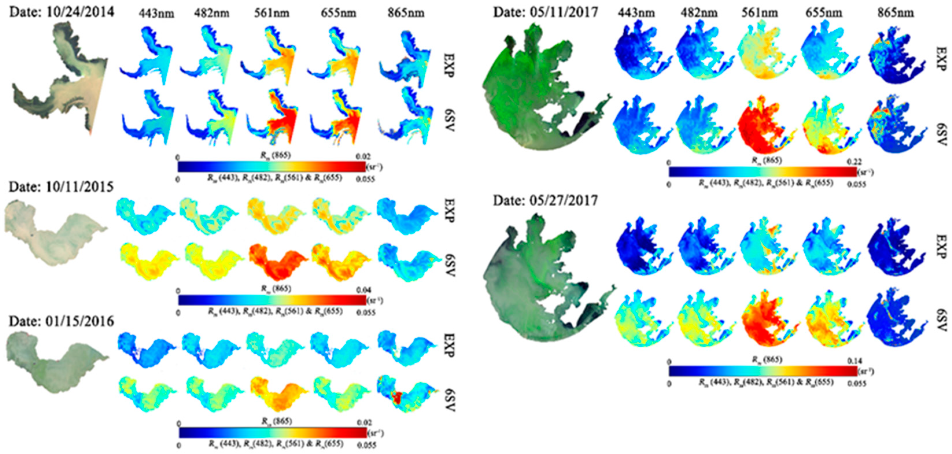
Figure 6.
Frequency of Rrs(λ) retrieved using EXP algorithm (blue line) and 6SV algorithm (red line) from OLI measurements in Lake Hongze on 24 October 2014, Lake Chaohu on 15 October 2015, January 11, 2016, and Lake Taihu on 11 May 2017 and 27 May 2017, respectively.
Figure 6.
Frequency of Rrs(λ) retrieved using EXP algorithm (blue line) and 6SV algorithm (red line) from OLI measurements in Lake Hongze on 24 October 2014, Lake Chaohu on 15 October 2015, January 11, 2016, and Lake Taihu on 11 May 2017 and 27 May 2017, respectively.

Figure 7.
OLI true color image presenting, Rrs(λ) for Lake Hongze on 24 October 2014, Lake Chaohu on 15 October 2015, 11 January 2016, and Lake Taihu on 11 May 2017 and 27 May 2017, respectively. Rrs(λ) was derived by EXP and 6SV algorithm.
Figure 7.
OLI true color image presenting, Rrs(λ) for Lake Hongze on 24 October 2014, Lake Chaohu on 15 October 2015, 11 January 2016, and Lake Taihu on 11 May 2017 and 27 May 2017, respectively. Rrs(λ) was derived by EXP and 6SV algorithm.

Figure 8.
Scatter plots of SPM calibration between in situ measurement data and SPM model (a), validation between measured and simulated Rrs-based derived measurements (b).
Figure 8.
Scatter plots of SPM calibration between in situ measurement data and SPM model (a), validation between measured and simulated Rrs-based derived measurements (b).

Figure 9.
OLI true color image, and distribution of estimated SPM patterns in Lake Chaohu on 15 October 2015, 11 January 2016. OLI-estimated SPM derived by EXP (a,c) and 6SV (b,d), and frequency of OLI-estimated SPM on 15 October 2015 (f) and 11 January 2016 (g), blue line was driven by EXP algorithm and red line was driven by 6SV algorithm. The comparison of in situ-measured SPM and OLI-estimated SPM derived by EXP and 6SV (e).

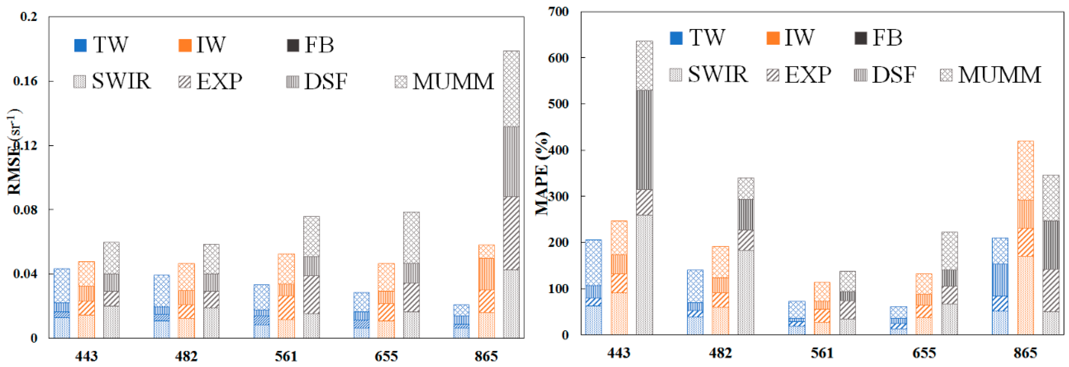
Figure 10.
Distribution of RMSE (right) and MAPE (left) of bands on different water types. Blue is TW (turbid water), orange is IW (in-water algae) and black is FB (floating bloom). The different patterns of column represent different water-AC algorithms.
Figure 10.
Distribution of RMSE (right) and MAPE (left) of bands on different water types. Blue is TW (turbid water), orange is IW (in-water algae) and black is FB (floating bloom). The different patterns of column represent different water-AC algorithms.

Figure 11.
Distribution of RMSE (right) and MAPE (left) of bands on different water types used for land-AC algorithms. Blue is TW (turbid water), orange is IW (in-water algae), and black is FB (floating bloom). The different patterns of column represent different land-AC algorithms.
Figure 11.
Distribution of RMSE (right) and MAPE (left) of bands on different water types used for land-AC algorithms. Blue is TW (turbid water), orange is IW (in-water algae), and black is FB (floating bloom). The different patterns of column represent different land-AC algorithms.

Figure 12.
OLI-RGB images and Rayleigh-corrected reflectance (ρrc) images of two SWIR bands in Lake Taihu (a,c,d) and Lake Chaohu (b,e,f). The Rayleigh-corrected reflectance derived by SeaDAS processing. (g) and (h) were line graphs of ρrc value from figure (a) and (b) (100 × 100 pixel area), respectively.

Figure 13.
The frequency of seasonal variation of aerosol types in Lake Taihu from 2005 to 2018. The HA, MA, SA, and HS represent highly absorbing, moderately absorbing, slightly absorbing, and highly scattering fine-mode aerosols, respectively.
Figure 13.
The frequency of seasonal variation of aerosol types in Lake Taihu from 2005 to 2018. The HA, MA, SA, and HS represent highly absorbing, moderately absorbing, slightly absorbing, and highly scattering fine-mode aerosols, respectively.


Table 1.
Bands of the OLI (Operational Land Imager) on Landsat-8, with band range, band center, ground sampling distance (GSD), and signal-to-noise ratio (SNR) at reference radiance [27].
Table 1.
Bands of the OLI (Operational Land Imager) on Landsat-8, with band range, band center, ground sampling distance (GSD), and signal-to-noise ratio (SNR) at reference radiance [27].
| Band | Band Range (nm) | Band Center (nm) | GSD (m) | SNR at Reference L |
|---|---|---|---|---|
| Band1 Coastal/Aerosol | 433–453 | 443 | 30 | 232 |
| Band 2 Blue | 450–515 | 482 | 30 | 355 |
| Band 3 Green | 525–600 | 561 | 30 | 296 |
| Band 4 Red | 630–680 | 655 | 30 | 222 |
| Band 5 NIR | 845–885 | 865 | 30 | 199 |
| Band 6 SWIR 1 | 1560–1660 | 1609 | 30 | 261 |
| Band 7 SWIR 2 | 2100–2300 | 2201 | 30 | 326 |
| Band 8 Pan | 500–680 | 590 | 15 | 146 |
| Band 9 Cirrus | 1360–1390 | 1375 | 30 | 162 |
Table 2.
The match-up dates of in situ measurement and OLI data acquisition over lakes Hongze, Chaohu, and Taihu.
Table 2.
The match-up dates of in situ measurement and OLI data acquisition over lakes Hongze, Chaohu, and Taihu.
| OLI Image | Acquisition Date | in situ Number | |
|---|---|---|---|
| Lake Hongze | LC81210372014297 | 24 October 2014 | 10 |
| Lake Chaohu | LC81210382015284 | 11 October 2015 | 15 |
| LC81210382016015 | 15 January 2016 | 16 | |
| Lake Taihu | LC81190382017131 | 11 May 2017 | 11 |
| LC81190382017147 | 27 May 2017 | 22 |
Table 3.
Variations of bio-optical properties of the three study lakes (Lake Hongze, Lake Chaohu, and Lake Taihu). The unit for Chla is μg/L. The units for SPOM and SPIM are mg/L.
Table 3.
Variations of bio-optical properties of the three study lakes (Lake Hongze, Lake Chaohu, and Lake Taihu). The unit for Chla is μg/L. The units for SPOM and SPIM are mg/L.
| Lake | Parameters | Minimum | Maximum | Mean | SD |
|---|---|---|---|---|---|
| Lake Hongze (n = 10) | Chla | 7.35 | 19.21 | 11.62 | 3.33 |
| SPOM | 6.00 | 11.33 | 8.67 | 1.61 | |
| SPIM | 28.00 | 47.33 | 35.33 | 6.68 | |
| SPOM/SPIM | 0.16 | 0.40 | 0.25 | 0.07 | |
| ag(440) | 1.19 | 1.59 | 1.38 | 0.13 | |
| aph(665) | 0.16 | 0.25 | 0.19 | 0.03 | |
| Lake Chaohu (n = 31) | Chla | 9.86 | 687.14 | 140.68 | 184.01 |
| SPOM | 8.00 | 216.00 | 38.53 | 48.08 | |
| SPIM | 8.00 | 93.00 | 40.94 | 27.93 | |
| SPOM/SPIM | 0.15 | 9.82 | 1.39 | 1.94 | |
| ag(440) | 0.79 | 1.75 | 1.22 | 0.27 | |
| aph(665) | 0.13 | 8.48 | 1.31 | 1.81 | |
| Lake Taihu (n = 33) | Chla | 19.96 | 1022.53 | 206.13 | 267.93 |
| SPOM | 4.00 | 321.33 | 72.04 | 85.48 | |
| SPIM | 13.33 | 88.00 | 44.14 | 16.80 | |
| SPOM/SPIM | 0.12 | 6.51 | 1.67 | 1.76 | |
| ag(440) | 0.46 | 3.28 | 1.16 | 0.60 | |
| aph(665) | 0.34 | 26.95 | 3.48 | 5.80 |
Table 4.
Variations in bio-optical properties of three water types (turbid water, in-water algae, and floating bloom). The unit for Chla is μg/L. The units for SPOM and SPIM are mg/L.
Table 4.
Variations in bio-optical properties of three water types (turbid water, in-water algae, and floating bloom). The unit for Chla is μg/L. The units for SPOM and SPIM are mg/L.
| Lake | Parameters | Minimum | Maximum | Mean | SD |
|---|---|---|---|---|---|
| Turbid water (n = 20) | Chla | 7.35 | 91.72 | 28.10 | 22.57 |
| SPOM | 6.00 | 34.00 | 14.77 | 8.09 | |
| SPIM | 28.00 | 93.00 | 52.44 | 20.34 | |
| SPOM/SPIM | 0.12 | 0.47 | 0.28 | 0.10 | |
| ag(440) | 0.89 | 1.75 | 1.36 | 0.24 | |
| aph(665) | 0.13 | 0.92 | 0.29 | 0.21 | |
| In-water algae (n = 38) | Chla | 19.96 | 687.14 | 104.39 | 125.78 |
| SPOM | 4.00 | 226.67 | 44.29 | 44.35 | |
| SPIM | 8.00 | 68.00 | 28.18 | 17.52 | |
| SPOM/SPIM | 0.23 | 8.67 | 1.57 | 1.96 | |
| ag(440) | 0.46 | 1.75 | 1.07 | 0.31 | |
| aph(665) | 0.31 | 16.43 | 1.89 | 3.01 | |
| Floating bloom (n = 16) | Chla | 103.86 | 1022.53 | 198.04 | 203.85 |
| SPOM | 25.33 | 321.33 | 117.27 | 69.46 | |
| SPIM | 16.00 | 88.00 | 44.91 | 20.17 | |
| SPOM/SPIM | 0.40 | 9.82 | 2.61 | 2.50 | |
| ag(440) | 0.37 | 3.28 | 2.62 | 1.04 | |
| aph(665) | 0.32 | 26.95 | 6.59 | 8.07 |
Table 5.
Band ratio errors between in situ Rrs and OLI Rrs obtained with atmospheric correction algorithms for water. The bold means the minimal statistical value and the underline means maximum.
Table 5.
Band ratio errors between in situ Rrs and OLI Rrs obtained with atmospheric correction algorithms for water. The bold means the minimal statistical value and the underline means maximum.
| Algorithm | Band Ratio | |||||||
|---|---|---|---|---|---|---|---|---|
| 443/561 | 482/561 | 655/561 | 865/561 | 443/655 | 482/655 | 865/655 | ||
| SWIR | RMSE | 0.3125 | 0.2180 | 0.0915 | 0.3916 | 0.3538 | 0.2339 | 0.7163 |
| MAPE (%) | 69.91 | 37.35 | 10.50 | 227.69 | 59.95 | 30.15 | 201.77 | |
| Bias (%) | 37.62 | 20.16 | 6.30 | −88.12 | 27.24 | 11.80 | −71.86 | |
| EXP | RMSE | 0.1758 | 0.1694 | 0.0971 | 0.7781 | 0.2099 | 0.1645 | 1.5130 |
| MAPE (%) | 54.48 | 30.93 | 10.65 | 197.08 | 46.11 | 21.59 | 195.52 | |
| Bias (%) | 24.72 | 21.20 | 6.53 | 42.88 | 15.10 | 12.60 | 63.03 | |
| DSF | RMSE | 0.19 | 0.1577 | 0.0984 | 0.6372 | 0.1951 | 0.1406 | 1.0799 |
| MAPE (%) | 88.91 | 29.31 | 11.31 | 130.87 | 61.72 | 17.23 | 132.07 | |
| Bias (%) | 85.08 | 26.18 | 8.06 | 120.54 | 59.08 | 15.00 | 118.22 | |
| MUMM | RMSE | 0.5013 | 0.3888 | 0.1656 | 0.4601 | 0.7234 | 0.5489 | - |
| MAPE (%) | 91.19 | 57.73 | 17.54 | 89.43 | 101.08 | 63.13 | - | |
| Bias (%) | −86.60 | −53.97 | 4.36 | −89.28 | −97.62 | −60.88 | - | |
Table 6.
Band ratio errors between in situ Rrs and OLI Rrs obtained with the land-AC algorithms. The bold means the minimal statistical value and the underline means maximum.
Table 6.
Band ratio errors between in situ Rrs and OLI Rrs obtained with the land-AC algorithms. The bold means the minimal statistical value and the underline means maximum.
| Algorithm | Band Ratio | |||||||
|---|---|---|---|---|---|---|---|---|
| 443/561 | 482/561 | 655/561 | 865/561 | 443/655 | 482/655 | 865/655 | ||
| FLAASH | RMSE | 0.3422 | 0.1876 | 0.0861 | 0.6970 | 0.3994 | 0.1908 | 1.1892 |
| MAPE (%) | 131.05 | 34.72 | 9.85 | 237.69 | 108.43 | 24.52 | 229.94 | |
| Bias (%) | 129.99 | 30.50 | 6.16 | 35.80 | 108.10 | 21.24 | 51.04 | |
| 6SV | RMSE | 0.2363 | 0.1697 | 0.0774 | 0.6360 | 0.2885 | 0.1907 | 1.1338 |
| MAPE (%) | 84.97 | 30.49 | 8.26 | 162.83 | 72.14 | 23.71 | 168.78 | |
| Bias (%) | 76.91 | 24.47 | 3.14 | 39.20 | 65.26 | 19.03 | 54.70 | |
| QUAC | RMSE | 0.2246 | 0.1849 | 0.0963 | 0.7539 | 0.2445 | 0.1880 | 1.1645 |
| MAPE (%) | 96.18 | 34.33 | 11.50 | 158.53 | 71.28 | 24.34 | 149.59 | |
| Bias (%) | 94.71 | 32.29 | 8.82 | 55.21 | 69.89 | 20.85 | 56.11 | |
© 2019 by the authors. Licensee MDPI, Basel, Switzerland. This article is an open access article distributed under the terms and conditions of the Creative Commons Attribution (CC BY) license (http://creativecommons.org/licenses/by/4.0/).
Share and Cite
MDPI and ACS Style
Wang, D.; Ma, R.; Xue, K.; Loiselle, S.A. The Assessment of Landsat-8 OLI Atmospheric Correction Algorithms for Inland Waters. Remote Sens. 2019, 11, 169. https://0-doi-org.brum.beds.ac.uk/10.3390/rs11020169
AMA Style
Wang D, Ma R, Xue K, Loiselle SA. The Assessment of Landsat-8 OLI Atmospheric Correction Algorithms for Inland Waters. Remote Sensing. 2019; 11(2):169. https://0-doi-org.brum.beds.ac.uk/10.3390/rs11020169
Chicago/Turabian StyleWang, Dian, Ronghua Ma, Kun Xue, and Steven Arthur Loiselle. 2019. "The Assessment of Landsat-8 OLI Atmospheric Correction Algorithms for Inland Waters" Remote Sensing 11, no. 2: 169. https://0-doi-org.brum.beds.ac.uk/10.3390/rs11020169
Note that from the first issue of 2016, this journal uses article numbers instead of page numbers. See further details here.