Superpixel-Guided Layer-Wise Embedding CNN for Remote Sensing Image Classification


1
Ministry of Education Key Laboratory for Earth System Modeling, Department of Earth System Science, Tsinghua University, Beijing 100084, China
2
Key Laboratory of Visual Perception and Artificial Intelligence of Hunan Province, College of Electrical and Information Engineering, Hunan University, Changsha 410082, China
3
School of Automation Science and Engineering, South China University of Technology, Guangzhou 510640, China
4
Ministry of Education Key Laboratory on Earth Surface Processes, Department of Ecology, College of Urban and Environmental Science, Peking University, Beijing 100871, China
*
Authors to whom correspondence should be addressed.
Remote Sens. 2019, 11(2), 174; https://0-doi-org.brum.beds.ac.uk/10.3390/rs11020174
Submission received: 30 November 2018
/
Revised: 9 January 2019
/
Accepted: 11 January 2019
/
Published: 17 January 2019
(This article belongs to the Special Issue Pattern Analysis and Recognition in Remote Sensing)
Abstract
:Irregular spatial dependency is one of the major characteristics of remote sensing images, which brings about challenges for classification tasks. Deep supervised models such as convolutional neural networks (CNNs) have shown great capacity for remote sensing image classification. However, they generally require a huge labeled training set for the fine tuning of a deep neural network. To handle the irregular spatial dependency of remote sensing images and mitigate the conflict between limited labeled samples and training demand, we design a superpixel-guided layer-wise embedding CNN (SLE-CNN) for remote sensing image classification, which can efficiently exploit the information from both labeled and unlabeled samples. With the superpixel-guided sampling strategy for unlabeled samples, we can achieve an automatic determination of the neighborhood covering for a spatial dependency system and thus adapting to real scenes of remote sensing images. In the designed network, two types of loss costs are combined for the training of CNN, i.e., supervised cross entropy and unsupervised reconstruction cost on both labeled and unlabeled samples, respectively. Our experimental results are conducted with three types of remote sensing data, including hyperspectral, multispectral, and synthetic aperture radar (SAR) images. The designed SLE-CNN achieves excellent classification performance in all cases with a limited labeled training set, suggesting its good potential for remote sensing image classification.
1. Introduction
Remote sensing images generally refer to the pictorial ground information acquired by satellite or aircraft sensor technologies. With sufficient spectral and spatial information, remote sensing images have played an important role in many applications, such as urban planning, agriculture management, climate monitoring, military affairs, etc. [1,2,3], while for these applications, classification with a fine accuracy is essential [4]. Different from common optical images, classifying remote sensing images is more difficult concerning their characteristics, such as having more spectral bands, rich spatial information, low spatial resolution, and so on [5,6]. Furthermore, remote sensing images usually have complex ground scenes and irregular objects, thus they are characteristic of irregular spatial dependency [7], which further cause challenges for classification tasks.
There have been many methods designed for the classification of remote sensing images, which can be roughly grouped into three categories, i.e., supervised, semi-supervised and unsupervised methods [8], according to the manner of the information exploration from labeled or unlabeled samples. On the one hand, unsupervised methods, generally using clustering strategies, such as fuzzy clustering [9] and fuzzy C-Means algorithms [10], which attempt to explore patterns from unlabeled samples [11], have been proved to be efficient but incapable of bridging the gap between clusters and classes [12]. On the other hand, supervised classifiers, such as support vector machine (SVM) [13,14], multinomial logistic regression [15,16] and artificial neural networks (ANN) [17,18], which learn from labeled samples to obtain prior knowledge, have demonstrated impressive performance. However, supervised classifiers heavily rely on the quantity and quality of labeled samples [19,20,21]. In real scenarios, sample labeling is usually difficult, time-consuming, and expensive [22]. Therefore, the labeled samples available are often insufficient, which leads to the occurrence of Hughes phenomenon [23] and increases the possibility of overfitting [24,25].
Semi-supervised learning is usually used to relieve the conflict between training demand and limited labeled sample set. It aims to make use of both limited labeled samples and abundant unlabeled samples, binds together unsupervised and supervised learning [26]. There exist many semi-supervised approaches in the literatures [27]. For instance, generative semi-supervised learning methods use the conditional density to determine labels of unlabeled samples [28,29,30]. However, those methods generally under the assumption that unlabeled samples follow a certain distribution which may limit the performance [11]. Wrapper methods include self-training [22,31,32] and co-training [22,33,34,35]. The former trains the classifier iteratively with new training samples labeled by the classifier itself, while the latter employ several classifiers to train with independent subsets of samples and the unlabeled samples with high reliability are then used to train another classifier. Self-training schemes may reinforce its poor predictions, while co-training algorithms demand that the samples can be divided into independent subsets [11]. Low-density separation algorithms, such as the transductive SVMs [36,37,38] which perform the classification by maximizing the margin for labeled and unlabeled samples, also suffer from the poor generalization ability. Graph-based approaches construct graphs to connect similar observations and spread labeled information in its neighbors by finding minimum energy function [12,39,40,41,42], which also incur some problems such as being sensitive to the graph structure [43,44].
Recently, deep learning structures have attained great success owing to its outstanding generalization capacity compared with traditional shallow structures [45]. Some of the recent developments are focused on semi-supervised learning, which exploits both labeled and unlabeled information to tackle the issue of overfitting, i.e., a limited number of labeled information and huge number of parameters involved [46]. This new trend has been successfully applied for remote sensing image classifications. For instance, Ma et al. [11] use a deep hierarchical structure to learn highly discriminative representation and pre-labels unlabeled samples, where multi-decision schemes are formed to update the labeled training data set and thus realize semi-supervised learning. However, this kind of purely discriminative and self-learning style semi-supervised way often rely on iterative training, thus are time-consuming and resource-consuming. He et al. [8] apply popular GANs (Generative adversarial networks) to study the latent representation of the input data, whose model resorts to the regularization techniques to explore the information in unlabeled samples and hence assist the discriminative classification tasks. In that generative model, unsupervised embeddings or hidden representations are often used to help supervised objectives [47]. Nevertheless, such latent variable models are still not suitable enough to match hidden representation with supervised tasks at hand. Rasmus et al. [48] propose a Ladder Network by combining supervised learning with unsupervised learning in deep neural networks, which needs only a small number of labeled samples. However, the method lacks the mining to spatial information of unlabeled samples, which weakens its capacity and applications, especially for remote sensing images.
Remote sensing images have complex ground scenes and irregular objects; thus, they are naturally characteristic of irregular spatial dependency [7], causing difficulties for classification. Deep supervised models such as CNNs are robust classifiers but require many training samples for fine tuning the network parameters, which conflicts with the reality that only a small number of labeled samples are available. To address these challenges, in this paper, we design a superpixel-guided layer-wise embedding CNN framework (SLE-CNN) for remote sensing image classification. It can automatically determine the neighborhood covering for a spatial dependency system and thus provide more a priori information of high quality for labels, which can improve the training performance of the deep network in a semi-supervised manner. We use a superpixel-based random sampling strategy to select unlabeled samples since superpixels are adaptive to real scenes of remote sensing images [7]. The involved layer-wise embedding CNN can fuse deep autoencoder (AE) and CNN in a layer-wise embedding fashion where unsupervised reconstruction cost and supervised cross entropy loss are optimized simultaneously, thus achieving an end-to-end structure. This structure can use information from both labeled and unlabeled samples and efficiently reduce the overfitting risks, therefore, well adapting to semi-supervised tasks. Moreover, instead of applying the unsupervised auxiliary tasks as only a part of pre-training procedure followed by normal supervised learning, the layer-wise embedding CNN shares the hidden representations between unsupervised generative representation and its discriminative counterpart, thus helps more informative unsupervised features to be learned for a discriminative purpose. All the above aspects contribute to the better classification performances for remote sensing images.
The main research objectives of this paper can be identified as follows:
- Considering the fact that remote sensing images are characteristic of irregular spatial dependency, we introduce the superpixel sampling strategy to guide the use of unlabeled samples, which can achieve an automatic determination of the neighborhood covering for a spatial dependency system and thus adapting to real scenes of remote sensing images. With the aid of these highly representative and informative unlabeled samples, the training process will be boosted, leading to better classification results.
- Deep CNNs are efficient classifiers, but it requires many labeled samples for training which conflicts with the reality that only limited labeled samples are available. To reduce the demand for labeled samples, we develop an SLE-CNN, which can take advantage of many unlabeled samples with the guide of superpixel-based random sampling. It regards CNN as the encoder part of the AE model and appends a reconstruction loss at each layer of the network that plays a role of extra supervision, thus combining the strong generalization capacity of deep CNN model with the detail preserving ability of AE.
- To demonstrate the performance of our framework for classification tasks of different types of remote sensing data, we conducted experiments to provide the latest results on benchmark problems. In addition, we compared our framework with several typical semi-supervised and supervised methods, which also verifies the effectiveness of our proposed framework.
The remainder of the paper is organized as follows. Section 2 presents our newly developed framework in detail. Experimental results with hyperspectral, multispectral and SAR image data are shown in Section 3. Some discussions with extra experiments are placed in Section 4. Finally, Section 5 draws some conclusions.
2. Methodology
The block diagram of the proposed classification framework for remote sensing images is shown in Figure 1. The core of the framework is SLE-CNN (shown in the purple block in Figure 1), which is mainly composed of two sequential steps: heuristic sampling based on superpixel segmentation and the layer-wise embedding CNN. To exploit the full potential of remote sensing data, both limited labeled samples and sufficient unlabeled samples are used to construct a training dataset. Considering the irregular spatial dependency in remote sensing images, the random sampling strategy based on superpixels is employed to guide the selection of unlabeled samples. Superpixels are adaptive to real scenes of remote sensing images, which can improve the performance of the framework considering the variations of spatial characteristics of remote sensing images. Samples close to superpixel boundaries, viewed as samples likely to be class boundaries with difficulty to distinguish, are of high representativeness and entropy and can strengthen the generalization capacity of classifiers. Unlabeled samples along with a limited size of labeled samples are subsequently organized in the form of patches and both input to the layer-wise embedding CNN to fine tune the deep network and search for the best generalization of the input data. At last, classification maps can be obtained through the input of patches from remote sensing images to the fine-tuned layer-wise embedding CNN.
In this section, we will thoroughly present structure of SLE-CNN. In the first two parts, we will first introduce the basic background and knowledge of the proposed method, including the detailed description of the proposed superpixel-based random sampling strategy for unlabeled samples in Section 2.1 and the structure of an autoencoder, one of the basic architectures used in our classifier, in Section 2.2. At last, in Section 2.3, we will illustrate the whole structure of the designed SLE-CNN in detail.
2.1. Superpixel-Based Random Sampling
To ensure both the representative ability and efficiency, we need to bring in a random sampling strategy to select just a portion of unlabeled dataset instead of using them all during the training process. However, absolute random strategy is not enough to exploit the potential of the unlabeled samples. To deal with this, we design a superpixel-based random sampling strategy.
Pixels close to the class boundaries usually have a higher error probability to be misclassified, which makes it informative for sample collection. After a beforehand segmentation, we can actually obtain a strong prior on both spectral and spatial domain. In addition, samples close to the boundaries are more likely to be those near the class boundaries. We can strengthen the generalization capacity of classifiers by taking into account these high entropy samples [49].
Considering the irregular spatial dependency of remote sensing images, we use superpixels segmentation to produce the segmentation results in view of its adaptive ability to different scenes of remote sensing images.
Simple Linear Iterative Clustering (SLIC) [50,51] algorithm is used as the method to obtain superpixels mainly considering its efficient computational performance compared to other algorithms. SLIC, which is a simple and efficient segmentation method based on k-means clustering, generates superpixels by clustering pixels in both spectral and spatial domains with each pixel linked to a feature vector :
where is the spectral vector at position . is a coefficient to balance the spectral and spatial components of the vector, . S is the nominal size of superpixels, and c is a variable to control the compactness of superpixels.
The algorithm starts by dividing image into tiles (, where and are the number of rows and columns in an image, respectively. is the expected spatial size of superpixels. represents ceiling function which maps a number to the least integer greater than or equal to the number) with initial cluster center () (). To avoid placing centers at edges and selecting noisy pixels, the cluster centers are moved in a window with the lowest gradient. The gradient is defined as:
where is the norm.
Then the superpixels are obtained by k-means clustering, where each pixel is assigned to the nearest initial cluster center, and a new center is recomputed as the average of the feature vectors of pixels belonging to the cluster. The process is iteratively repeated until convergence. After the k-means clustering, the SLIC algorithm assigns disjoint segments to the largest neighboring cluster to enforce connectivity.
Based on the SLIC algorithm, we can sample the most representative unlabeled data. With simple random sampling strategy, samples are selected randomly and may be biased, which cannot meet the need for semi-supervised learning [52]. To select highly informative unlabeled samples automatically and reduce the demand of enlarging training samples, we introduce a superpixel segmentation-based random sampling strategy, which can also be regarded as a process to mine samples that are hard to distinguish:
- Images are segmented to superpixels, and all pixels in images are recorded as set A;
- Randomly choose a part of set A as set B;
- Pixels located on the boundaries of superpixels are detected and recorded as set C;
- For each pixel in set B, if its spatial distance to any pixel of the same superpixel in set C is less than or equal to k (pixel unit), put it in the candidate list.
This whole sampling procedure can be visualized as Figure 2.
2.2. Autoencoder
An autoencoder (AE) is an artificial neural network used for unsupervised learning of efficient codings [53,54]. An AE aims to learn a representation (encoding) for a set of data.
Architecturally, the simplest form of an AE is a feedforward, non-recurrent neural network very similar to the multilayer perceptron (MLP)—having an input layer, an output layer and one or more hidden layers connecting them—but with the output layer having the same number of nodes as the input layer, and with the purpose of reconstructing its own inputs.
An AE always consists of two parts, the encoder and the decoder. In the simplest case, where there is one hidden layer, the encoder stage of an AE takes the input x and maps it to r
where the image r is usually referred to as code, latent variables, or latent representation. is an element-wise activation function such as a sigmoid function or a rectified linear unit (ReLU). W is a weight matrix and b is a bias vector.
After the encoder, the decoder stage of the AE maps r to the reconstruction of the same shape as x
where , and for the decoder may differ in general from the corresponding , W and b for the encoder, depending on the design of the AE.
AEs are also trained to minimize reconstruction costs (such as square error):
where x is usually averaged over some input training set.
Denoising AEs take a partially noisy input while training to recover the original clean input. This technique has been introduced with a specific approach to good representation [55]. A good representation is one that can be obtained robustly from a noisy input and that will be useful for recovering the corresponding clean input.
2.3. Superpixel-Guided Layer-Wise Embedding CNN
Remote sensing images have complex ground scenes and irregular objects, thus irregular spatial dependency is one of the major characteristics of remote sensing images, which brings about challenges for classification tasks. Though prevailing deep supervised models usually have good feature generalization capacities with sufficient training samples, the situation will deteriorate rapidly when labeled data is limited [56]. This dilemma originates from the conflict between huge parameter volume and insufficient training samples. To handle the irregular spatial dependency and relieve the training demand for labeled samples, we design a superpixel-guided layer-wise embedding CNN framework to assist the optimization process for remote sensing image classification introducing the use of unlabeled data.
Since the goal of using unlabeled data for unsupervised learning is actually a type of regularization for supervised learning, we expect our supervised tasks to perform better, which demand the hidden representations shared by both supervised and unsupervised parts to be more robust. To achieve this, we need on one hand to feed more informative training samples to learn the best representation, and on the other hand to design a more powerful network structure to capture the internal characteristics of the input data. For the latter, we establish a layer-wise embedding CNN structure to efficiently learn the best discriminate feature for final classification. For the former, we use the superpixel-based random sampling strategy (as introduced in Section 2.1) to heuristically search useful and informative unlabeled samples without enlarging the labeled part of the training dataset. In particular, superpixels are usually spatially irregular subregions, but pixels inside them are homogenous, which means an automatic determination of the neighborhood covering for a spatial dependency system in a data-dependent manner [7]. Thus, supepixels are adaptive to real scenes of remote sensing images considering the irregular spatial dependency in remote sensing images.
The proposed whole SLE-CNN structure is shown in Figure 3, where all the inputs are organized as patches from pixels. Superpixel-guided patches, referring to unlabeled samples which are selected under the superpixel-based random sampling strategy shown in the left purple block of the figure, along with labeled patches are input to the layer-wise embedding CNN in the right part of the figure to fine tune the network. To get a classification map for a remote sensing image, each patch from each pixel need to be input to the fine-tuned layer-wise embedding CNN so that a class label at each pixel can be obtained, shown in the upper part of the figure with an orange-red color arrow.
From the denoising AE’s point of view, the layer-wise embedding CNN can be constructed by two parts in sequence, where two versions of encoder architectures, including one clean encoder (the green block in the top of Figure 3) and one noisy encoder (the blue block at the bottom of Figure 3), are followed by a mutual decoder architecture (the yellow block in the middle of Figure 3). Here, noise is injected into hidden layers of the noisy encoder to obtain a better feature generalization, which is similar to the common regularization technique dropout [57]. Specifically, we use a deep spectral-spatial CNN structure, which can make full use of spectral and spatial information of remote sensing images, as the architectures of the encoders to enhance the representative capacity and increase the supervised discriminative power. The parts of the structure are associated through skip connection and layer-wise embedding structures. The former technique strengthens the representative ability of the learned feature in the reconstruction stage by the superposition of the noisy encoder part upon the decoder part layer-wisely. The latter one serves as an extra supervision for the joint optimization process to achieve a strong regularization for raw remote sensing images and promote the discriminative ability.
Consider a dataset with labeled samples and unlabeled samples where . The goal for the classifier is to learn a function that models by using both the labeled samples and the unlabeled samples. Here, the objective function for the training of the layer-wise embedding CNN is casted as a sum of the supervised cross entropy ( in Figure 3) related to labeled patches from the noisy encoder and the unsupervised reconstruction cost ( in Figure 3) from superpixel-guided unlabeled patches at each layer of the decoder. Since all layers of the noisy encoder are corrupted by noise, another clean encoder path with shared parameters is responsible for providing the clean reconstruction targets. The whole structure is optimized by traditional backpropagation gradient descent.
At the end of the encoder path, we can obtain the one-hot encoded classification vector through a full connection layer combined with SoftMax operation. Please note that the ultimate class label for each input patch of remote sensing images at the test stage comes from the clean output from the clean encoder, while the noisy output from the noisy encoder is only for calculating the supervised cross entropy.
Each part of the layer-wise embedding CNN is explained in detail in the following.
2.3.1. General Steps for Constructing Layer-Wise Embedding CNN
Based on the structure of a denoising AE, we combine a noisy encoder and corresponding decoder layer via vertical skip connections, where two signals are fused by a denoising function to reconstruct the layer in the decoder. This technique helps the higher layer to focus on extracting more abstract and task-specific features, which can facilitate feature extraction from complex remote sensing images. Meanwhile, a clean encoder is trained in a feedforward fashion to evaluate the reconstruction effect [58].
The layer-wise embedding CNN can be defined as (suppose we have a total of L layers in both encoder and decoder parts):
where , and represent the noisy encoder, the clean encoder, and the decoder, respectively. x, and are the clean, noisy, and reconstructed input patches, respectively. , , and are the clean hidden representation, its noisy version, and its reconstructed version at layer l. y and , outputs after SoftMax operation, are the clean class label and the noisy class label, respectively. The noisy is used to calculate supervised cross entropy during the training process as described in following Equation (17), while the classification map is obtained from the clean y at test stage.
2.3.2. CNN Based Encoder for Supervised Learning
To use both spectral and spatial information in remote sensing images and enhance the representative capacity, a spectral-spatial CNN structure is constructed into the encoder architecture in the forward path. Overall, the encoder consists of the convolution, max pooling, batch normalization, noise injecting (for the noisy encoder) and activation operations for each layer. At the end of the encoders, the output y and are obtained through SoftMax operation (see Figure 3).
Firstly, 3-D convolution and max pooling transformations from layer to layer l are put on , the post-activation at layer , to obtain the pre-normalization :
Batch normalization is then applied to with the mini-batch mean and standard deviation . In addition, isotropic Gaussian noise is added to compute pre-activation :
Then, through a nonlinear activation function such as ReLU, defined as , we can obtain , the post-activation at layer l, as the input for the next layer:
where and are trainable parameters responsible for shifting and scaling.
Please note that the above equations describe the noisy encoder, with noisy and . If we remove noise, we will obtain the clean version of the encoder with clean s and r.
2.3.3. Vertical Connection and Vanilla Combinator-Based Denoising Function for Unsupervised Learning
In the backward path, deconvolution, unpooling and batch normalization are performed at layers in the decoder. Besides, vanilla combinator-based denoising function is used for combining the signal from the noisy encoder and the signal in the decoder, which achieves the vertical connection. This technique strengthens the representative ability of the learned feature in the reconstruction stage.
For each layer of the decoder, deconvolution and unpooling operations from layer to layer l are employed to layer :
Batch normalization is then implemented on to get :
After normalization correction, the signal from the layer and the noisy via vertical connection are combined into the reconstruction through a denoising process:
where is the vanilla combinator-based denoising function. It can combine the lateral and the vertical connections in an element-wise fashion.
Here, function is to achieve the lowest reconstruction cost. Considering the conditional distribution that we intend to model, the optimal functional form of g will be linear with respect to when is Gaussian. The parametrization of the denoising function is therefore:
where we modeled both and with a multilayer architecture form nonlinear function: and . to are linear coefficients. For a given u, is linear related to the parametrization, and both v and depend nonlinearly on u.
2.3.4. Overall Objective Function Formulation
Finally, the objective function for the layer-wise embedding is a balance of the supervised cross entropy from the noisy encoder and the unsupervised reconstruction cost at each layer of the decoder. Since all layers of the noisy encoder are corrupted by noise for the purpose of obtaining a better feature generalization, the clean encoder is providing the clean reconstruction targets as the reference of the decoder.
The objective function, , is defined as the following shows:
where is supervised cross entropy from the noisy encoder and is unsupervised reconstruction costs from the decoder.
(with N labeled patches) is calculated as the sum negative log probability of the noisy output matching the target output given the input :
And (with M superpixel-guided unlabeled patches) represent the sum of reconstruction costs from all L layers:
where represents the layer-wise embedding unsupervised reconstruction cost which consists of cost from each decoder layer. is a layer-wise coefficient. The denoising intensity of each layer can be tuned by changing each .
in the above Equation (18) is formalized as:
where is performed batch normalization with mean and standard deviation of in the noisy encoder part.
The feedforward pass of the layer-wise embedding CNN is listed in Algorithm 1, where means batch normalization, and is the nonlinear activation function, such as ReLU.
| Algorithm 1 Calculation of output class labels and objective function of the layer-wise embedding CNN |
Require:
|
3. Experimental Setup
In this section, we use three different types of remote sensing images to evaluate our designed SLE-CNN framework. All of them are common benchmarks concerning their types. A series of experiments have been conducted to make a comprehensive comparison among various methods. All experiments are carried out with the same image pre-processing operations to guarantee fairness.
3.1. Dataset Description
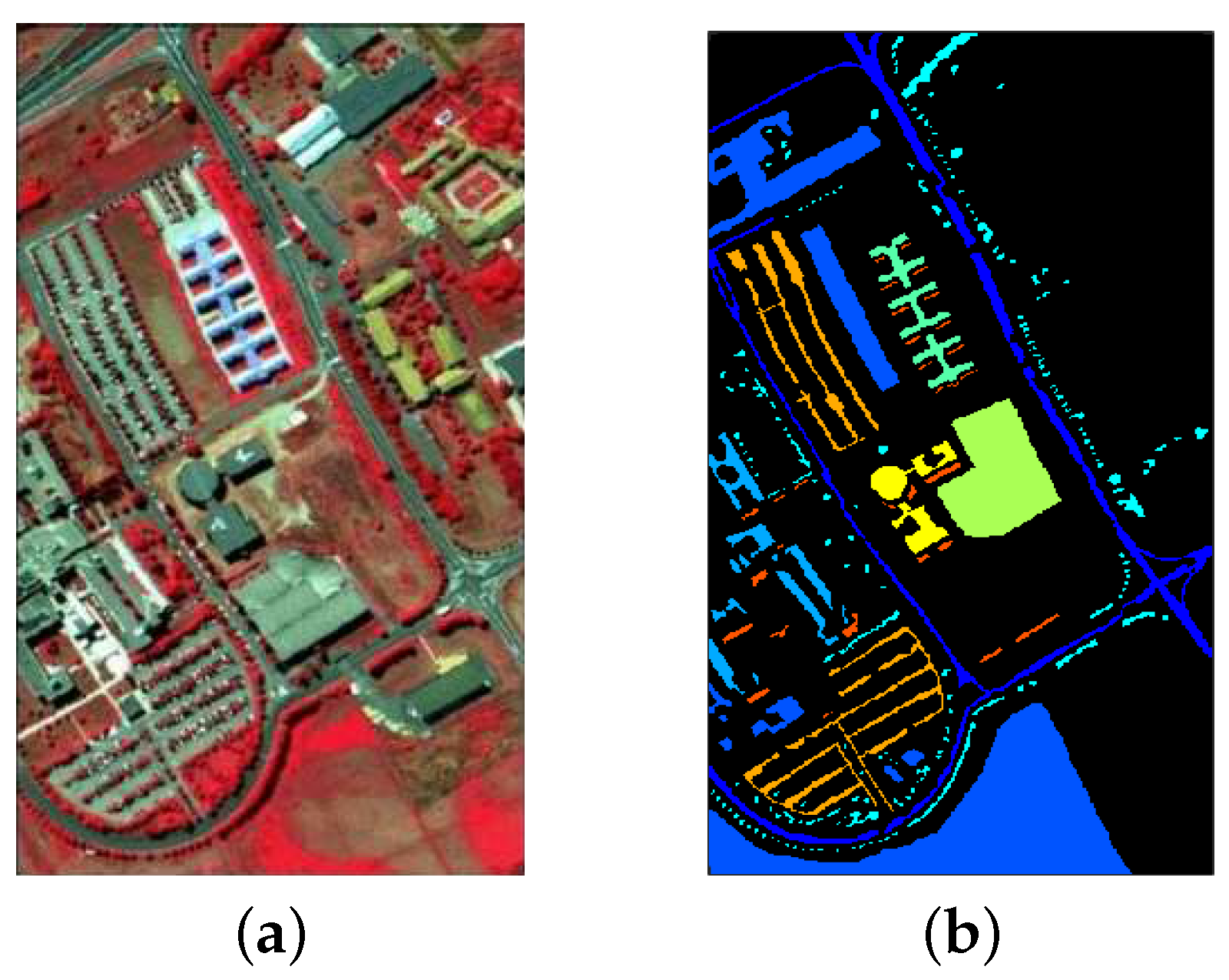
Hyperspectral image (HSI), acquired by hyperspectral imaging sensors, consists of hundreds or even thousands of continuous spectral bands, carrying abundant information. In the experiments, publicly available University of Pavia data (http://www.ehu.eus/ccwintco/index.php/Hyperspectral_Remote_Sensing_Scenes) is employed as a benchmark HSI dataset. It was captured by the Reflective Optics System Imaging Spectrometer (ROSIS) sensor over an urban area at the University of Pavia, Italy, in 2002. The image is composed of 610 × 340 pixels with a spatial resolution of 1.3 m. It contains 115 bands. After removing 12 noise bands, 103 bands are remaining. The ground truth map contains 9 classes. Figure 4 shows the false color image as well as the ground truth data. There are 9 classes of interest and the detailed information of each class is listed in Table 1.
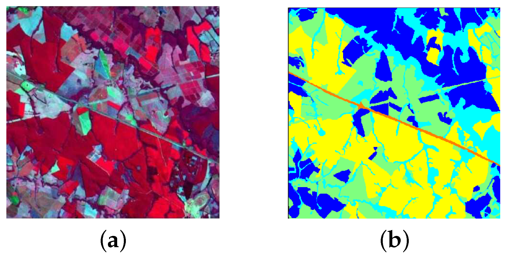
Multispectral image (MSI), acquired by multispectral sensors, contains several useful discontinuous spectral bands. One image (http://www.recogna.tech), covering the area of Itatinga, SP-Brazil, obtained by Landsat 5 TM, one of the most popular multispectral sensors, is used in the experiments. The image consists of 492 × 526 pixels and 3 bands. The ground truth map contains 6 classes, Figure 5 shows the ground truth data as well as the image. The 6 classes of interest and the detailed information of each class are listed in Table 2.
SAR imagery, acquired by synthetic aperture radar, carries a lot of speckle noise. Here, one image collected by Electromagnetics Institute Synthetic Aperture Radar (EMISAR) (http://www.space.dtu.dk/english/Research/Research_divisions/Microwaves_and_Remote_Sensing/Sensors/emisar) is used. It was captured over a vegetated region, in Foulum, Denmark. The image is composed of 421 × 300 pixels and 41 bands. Its ground truth map contains 5 classes, Figure 6 shows the ground truth data as well as the image. The 5 classes of interest and the detailed information of each class are listed in Table 3.
3.2. Experiments
To evaluate the designed SLE-CNN framework for remote sensing image classification, we compare it with the supervised version of our model and some other classification algorithms, i.e., SVM, Laplacian SVM (LapSVM), Self-learning (based on Breaking Ties or BT strategy) SVM (SL SVM), convolutional neural network - autoencoder (CNN-AE). Therein, supervised version of our framework with only cross entropy to learn, has the same structure with the encoder part of the semi-supervised version to ensure the comparability. Specifically, SVM is also in supervised fashion, while LapSVM and SL SVM are semi-supervised classifiers. The LapSVM [59], which is a graph-based semi-supervised learning method, introduces an additional manifold regularization term on the geometry of both the labeled and the unlabeled data using the graph Laplacian and has been demonstrated as an effective approach [60,61]. Self-learning is one of the traditional wrapper methods of semi-supervised learning. Here, SVM is chosen as the probabilistic classifier. In addition, the BT active learning algorithm [62], which focuses on searching the samples with the smallest difference between the two most probable classes, is combined with self-learning strategy to serve as an adaptive machine-machine approach. To compare with a contextual method, SL SVM is performed on both the original spectral data and the Gabor textures (with SL-Gabor SVM) [63]. CNN-AE is an approach based on convolutional features and sparse AE for remote sensing images, proposed by [64], whose architecture is a sequential version of our proposed method. This approach starts by generating an initial feature representation from a pre-trained CNN model. Then these convolutional features are fed into an AE for learning a new suitable representation in an unsupervised manner. After this, several class-specific AEs are trained, and the images are then classified based on the reconstruction error. To ensure the fairness, the CNN architecture implemented in CNN-AE is consistent with our proposed method (same number of layers, same size of filters and so on) as described behind. In addition, we have also used the superpixel-based sampling strategy in CNN-AE.
The experiments are implemented on the aforementioned three kinds of datasets. Following the procedure shown in Figure 1, 40% of the ground truth data is randomly selected for testing. Among the remaining part, a small number of labeled samples, 5 samples per class for HSI, SAR and MSI datasets, are selected from the training samples as labeled samples with a stratified random sampling strategy. Then the SLIC is implemented upon the whole remote sensing image with an average superpixel size of 400 pixel unit. Those pixels within 3 pixel unit distance to the boundary of its superpixel are selected as the candidate unlabeled samples, where those belong to test samples and labeled samples are removed. Then from the candidate unlabeled samples, 5000, 7000 and 3500 samples are randomly selected as the unlabeled samples for HSI, SAR and MSI datasets, respectively. Finally, both the unlabeled and labeled samples constitute the training set and used for network fine-tuning. Please note that we did not consider the spatial autocorrelation [65] of the input images during the process of separating training and testing samples. In addition, we organize samples in the form of patches. We train the LWE-CNN in random batches with a batch size of 16. All the evaluation experiments are repeated for 10 Monte Carlo runs, and the reported accuracy are the average results. To evaluate the experimental results, we compare three indexes, including overall accuracy (OA, the number of correct classifications by the total number of test samples) [66], average accuracy (AA, an average of the producer’s accuracy of individual classes) [67] and kappa coefficient (Kappa, a measure of the actual agreement minus chance agreement) [68]. Moreover, the F-Measure (, where P represents the user’s accuracy and R is the producer’s accuracy) [69] of various methods is also compared.
For parameter settings of the layer-wise embedding CNN, we adopt a simple structure of 4 convolution layers and 1 full connection layer as the encoder part while a structure of the same amount of convolution as the decoder counterpart. The hyper-parameters in each layer of layer-wise embedding CNN are set empirically and can be found in Table 4. The learning rate is set to be 0.001 with mini-batch size of 45 for HSI, 25 for SAR and 100 for MSI. Though hyper-parameters (such as the number of filters and layers, etc.) of both encoder and decoder has not been fully optimized, with the adopted empirical settings, the results obtained are already very competitive. Moreover, for different types of remote sensing images, there is still huge improvement space if we fine tune the hyper-parameters separately for HSI, MSI and SAR data.
3.3. Experimental Results and Discussions
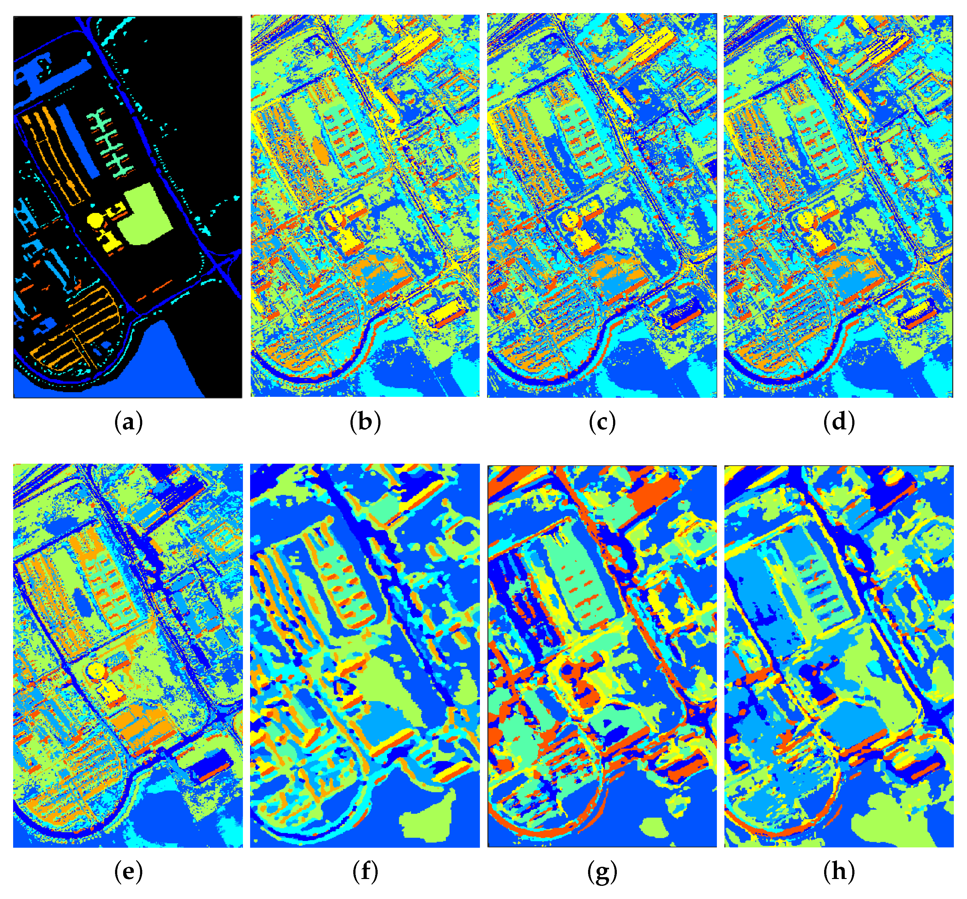
For illustrative purposes, Figure 7 show the OA as a function of the number of iterations in the fine-tuning process of SLE-CNN for the three different types of datasets, respectively. In the figures, the curves in the yellow color show the original results with fluctuation, while curves in the blue color are results through a certain percentage of smoothing. It can be observed that the designed SLE-CNN framework converges very fast, requiring merely 11, 8 and 11 times of iterations with a proper mini-batch size for HSI, MSI and SAR data respectively, which indicates its strong ability. The quantitative evaluations of the classification accuracy are shown in Table 5, Table 6 and Table 7. The classification maps are also visually as Figure 8, Figure 9 and Figure 10 show.
Based on the above-mentioned experimental results, a few discussions can be highlighted. Firstly, among the four SVM-based classifiers (SVM, LapSVM, SL SVM and SL-Gabor SVM), SVM using only the limited labeled data performs worst. For instance, it is observed from Table 7 that the OA of SVM is 10.17%, 8.18% and 11.01% lower than those of the LapSVM, SL SVM and SL-Gabor SVM, respectively. Similar properties can also be found in Table 6 and Table 7. This phenomenon demonstrates the importance of taking advantage of unlabeled data.
Secondly, compared with the designed SLE-CNN framework, the network structure of the supervised version of the proposed framework is simple, with only one encoder. In addition, it uses only supervised cross entropy for training while the SLE-CNN framework uses a combined loss function which consists of the supervised cross entropy from the noisy encoder and the unsupervised reconstruction cost from the interaction of the clean encoder and the decoder. From the experiments, we can see that the classification accuracy under supervised scenario is relatively worse than that obtained under SLE-CNN situation. As shown in Table 7, the OA, AA, Kappa and F-Measure of the supervised CNN are lower than those of the SLE-CNN, which again proves the efficiency and effectiveness of the unsupervised co-training fashion. It also implies that optimization with unlabeled data can reduce the error rate. To obtain a similar level classification accuracy, the need for labeled samples in our designed SLE-CNN framework is relatively lower than that of the supervised version.
Thirdly, even without unlabeled samples for training, deep structures such as CNN still have good-enough results reflected in high classification accuracy and smooth output classification map with little-shattered fragments, which outperforms traditional shallow models (e.g., SVM) with same training dataset. As shown in Table 5, the OA of purely supervised CNN is 5.94%, 1.23%, 3.27% and 0.01% higher than those of the SVM, LapSVM, SL SVM and SL-Gabor SVM, respectively. It is also clearly visible that little-shattered fragments are generated in purely supervised and SLE-CNN classification map in Figure 8 than in SVM, Laplacian SVM, SL SVM and SL-Gabor SVM classification map in Figure 8. The SAR data also yield similar properties. As for MSI data (see Table 7), the OA of the purely supervised CNN is lower than those of the LapSVM, SL SVM and SL-Gabor SVM but still higher than that of the SVM. To some extent, the classification maps of contextual methods (CNN and SL-Gabor SVM), though much smoother, lack a certain number of details, such as sharp corners and fine elements. However, some of the lost details may be noises caused by sensors.
Fourthly, when compared with SL-Gabor SVM, the designed SLE-CNN framework shows a higher accuracy, though both using unlabeled samples and contextual features, as shown in Table 5, Table 6 and Table 7, which further illustrates the capability of deep CNN.
Besides, the designed SLE-CNN framework performs better than CNN-AE with a different CNN architecture, which proves the superiority of the structure of our proposed model. As shown in Table 5, Table 6 and Table 7, the OA of the designed SLE-CNN framework is 3.13%, 1.88% and 2.33% higher than those of CNN-AE, respectively. Besides, the computation time of CNN-AE is longer than the designed SLE-CNN framework. The reasons may include: (1) In our proposed framework, end-to-end learning is used in the training process, where supervised and unsupervised parts are trained together through the cost function (Equation (16)) by backpropagation. (2) All classes are trained at the same time in our proposed framework. However, in CNN-AE, each class needs to be trained in a separate AE, respectively. (3) During the inference part, CNN-AE needs to run the pre-trained model to obtain CNN features and then runs AE t times (if we have t classes). While, in our proposed framework, the result can be acquired by running the encoder part of AE only one time. Finally, the designed SLE-CNN provides better or comparable classification results as compared with any other method included in comparison and obtain a state-of-art classification accuracy. Regarding all three different scenarios involving HSI, MSI and SAR data, which also demonstrates its strong adaptation capacity to adapt to different types of image classification tasks in the field of remote sensing.
Briefly, the aforementioned analysis validates the effectiveness of the SLE-CNN framework for remote sensing image classification.
4. Discussion
We further make experiments to verify the effectiveness of the designed superpixel-based random sampling strategy compared with totally random sampling strategy based on the layer-wise embedding CNN. Accuracy results based on 5 labeled samples per class are shown in Figure 11, which confirm the efficiency of the idea of superpixel-based random sampling. Overall, the above experimental results prove the superiority of our designed SLE-CNN framework for remote sensing image classification, considering both the sampling strategy and the deep network.
Also, we evaluate the performance of our designed SLE-CNN framework with the increase in the number of labeled samples and estimate its stability. We randomly choose 5, 10, 15, 20, 25 and 30 samples from each class as the labeled samples and the OA of above various methods is plotted in Figure 12, which shows that the classification accuracy increases as the number of labeled samples goes up and our designed SLE-CNN framework is superior to other methods when the same number of labeled training samples is chosen. Although the performance of different methods changes as the number of training samples changes, the designed SLE-CNN framework provides higher classification accuracies than other methods.
It should be noted that under the condition of extremely limited training samples, our framework has the risk of becoming unstable and influenced by noises, which need to be improved in the algorithm. However, the superpixel-based random sampling strategy, used for the guide of the selection of unlabeled samples, has reduced such risks to some degree. It should also be mentioned that classification results produced by the designed framework may be over-smooth and some details may be lost. Therefore, it should be treated carefully.
From the above Table 5, Table 6 and Table 7, we can observe the phenomenon that the accuracies of some classes of other methods are higher than those of our proposed SLE-CNN. The accuracies shown in the tables are under the condition of only 5 labeled samples per class, where the phenomena can in some degree reflect that our proposed SLE-CNN has the risk of becoming unstable and influenced by noises with extremely limited training samples as stated above. However, with the increase in the number of samples, the situation turns good. In Table 5, “bitumen” class of HSI data shows a relatively lower accuracy. However, the number of this class is small, so that the test results may be more likely to be interfered by randomness. As for “shadows” of HSI data in Table 5 and “winter wheat”, “water” classes of SAR data in Table 7, the accuracies of these classes, though not the highest among different methods, have already reached a high level. The relatively low accuracies of classes in MSI data in Table 6 reflect that our proposed SLE-CNN performed not so well on MSI data compared to HSI and SAR data under the condition of 5 labeled samples per class. Though the OA and other global indexes are still better than other methods, the improvement on accuracy is relatively small. Considering this, we will make some adaptive adjustments to the MSI data in later research.
In the future, we plan to combine variational inference with the unsupervised autoencoder model to obtain a better regularization for supervised learning and improve the decision boundaries. It is also promising to directly fuse the superpixel-based hard mining criterion into the final optimization objective.
5. Conclusions
Remote sensing images, with complex ground scenes and irregular objects, are naturally characteristic of irregular spatial dependency, which cause challenges for classification tasks. Moreover, effective labeled samples are usually scared in remote sensing datasets, which conflict with the general requirement of a huge labeled training set for the fine tuning of a deep neural network. To deal with these challenges, we design a superpixel-guided layer-wise embedding CNN framework, where unlabeled samples can be automatically exploited with the guide of a superpixel-based random sampling strategy. Therefore, a more robust training dataset can be obtained with many informative and representative unlabeled samples. Furthermore, since superpixels can handle the challenge of irregular spatial dependency, our classification framework is much more adaptive to real scenes of remote sensing images. Different from prevailing deep supervised learning models such as DNNs and CNNs that have already shown an impressive capacity for feature generalization with enough training samples, the designed SLE-CNN aims at relieving relevant problem under limited ground truth situations. By using AE-based generative model for learning unsupervised embedding of unlabeled samples, we can strongly regularize the supervised training, thus reducing the searching space to obtain a better convergency performance. In addition, since the supervised and unsupervised parts are combined in a joint optimization fashion with a new objective function, we can simultaneously learn the best feature representation with both supervised and unsupervised information. Experiments on benchmark remote sensing images of different types have shown satisfactory performances compared with both our framework in purely supervised manner and other state-of-art supervised and semi-supervised classification models, which implies a promising classification capacity for remote sensing images in different application fields.
Author Contributions
All coauthors made significant contributions to the manuscript. H.L., J.L. and L.H. designed the research framework, analyzed the results, and wrote the paper. Y.W. provided many constructive suggestions on the framework design and assisted in the preparatory work and validation work.
Funding
This work was supported in part by the National Natural Science Foundation of China under Grant 61571195, Grant 61771496, Grant 61633010 and Grant 61836003, in part by the Guangdong Provincial Natural Science Foundation under Grant 2016A030313254, Grant 2016A030313516 and Grant 2017A030313382, in part by the National Key Research and Development Program of China under Grant 2017YFB0502900, and in part by China Scholarship Council under Grant 201706155080.
Acknowledgments
The authors would like to thank Paolo Gamba from the University of Pavia for providing the ROSIS University of Pavia dataset, the Biometric and Pattern Recognition Research Group for providing the Landsat 5 TM dataset and the Technical University of Denmark for providing the EMISAR dataset.
Conflicts of Interest
The authors declare no conflict of interest.
References
- Young, O.R.; Onoda, M. Satellite Earth Observations in Environmental Problem-Solving. In Satellite Earth Observations and Their Impact on Society and Policy; Onoda, M., Young, O.R., Eds.; Springer: Singapore, 2017; pp. 3–27. [Google Scholar] [Green Version]
- Sun, B.; Kang, X.; Li, S.; Benediktsson, J.A. Random-walker-based Collaborative Learning for Hyperspectral Image Classification. IEEE Trans. Geosci. Remote Sens. 2017, 55, 212–222. [Google Scholar] [CrossRef]
- Yang, L.; Wang, M.; Yang, S.; Zhang, R.; Zhang, P. Sparse Spatio-Spectral LapSVM With Semisupervised Kernel Propagation for Hyperspectral Image Classification. IEEE J. Sel. Top. Appl. Earth Obs. Remote Sens. 2017, 10, 2046–2054. [Google Scholar] [CrossRef]
- Sharma, A.; Liu, X.; Yang, X.; Shi, D. A Patch-based Convolutional Neural Network for Remote Sensing Image Classification. Neural Netw. 2017, 95, 19–28. [Google Scholar] [CrossRef] [PubMed]
- Plaza, A.; Benediktsson, J.A.; Boardman, J.W.; Brazile, J.; Bruzzone, L.; Camps-Valls, G.; Chanussot, J.; Fauvel, M.; Gamba, P.; Gualtieri, A.; et al. Recent Advances in Techniques for Hyperspectral Image Processing. Remote Sens. Environ. 2009, 113, S110–S122. [Google Scholar] [CrossRef]
- Richards, J.A.; Jia, X. Remote Sensing Digital Image Analysis: An Introduction, 3rd ed.; Springer: Berlin/Heidelberg, Germany, 1999. [Google Scholar]
- He, L.; Li, J.; Liu, C.; Li, S. Recent Advances on Spectral-spatial Hyperspectral Image Classification: An Overview and New Guidelines. IEEE Trans. Geosci. Remote Sens. 2018, 56, 1579–1597. [Google Scholar] [CrossRef]
- He, Z.; Liu, H.; Wang, Y.; Hu, J. Generative Adversarial Networks-Based Semi-Supervised Learning for Hyperspectral Image Classification. Remote Sens. 2017, 9, 1042. [Google Scholar] [CrossRef]
- Zhong, Y.; Ma, A.; Zhang, L. An Adaptive Memetic Fuzzy Clustering Algorithm With Spatial Information for Remote Sensing Imagery. IEEE J. Sel. Top. Appl. Earth Obs. Remote Sens. 2014, 7, 1235–1248. [Google Scholar] [CrossRef]
- Niazmardi, S.; Homayouni, S.; Safari, A. An Improved FCM Algorithm Based on the SVDD for Unsupervised Hyperspectral Data Classification. IEEE J. Sel. Top. Appl. Earth Obs. Remote Sens. 2013, 6, 831–839. [Google Scholar] [CrossRef]
- Ma, X.; Wang, H.; Wang, J. Semisupervised Classification for Hyperspectral Image based on Multi-decision Labeling and Deep Feature Learning. ISPRS J. Photogramm. Remote Sens. 2016, 120, 99–107. [Google Scholar] [CrossRef]
- Camps-Valls, G.; Marsheva, T.V.B.; Zhou, D. Semi–Supervised Graph-Based Hyperspectral Image Classification. IEEE Trans. Geosci. Remote Sens. 2007, 45, 3044–3054. [Google Scholar] [CrossRef]
- Gao, L.; Li, J.; Khodadadzadeh, M.; Plaza, A.; Zhang, B.; He, Z.; Yan, H. Subspace-Based Support Vector Machines for Hyperspectral Image Classification. IEEE Geosci. Remote Sens. Lett. 2014, 12, 349–353. [Google Scholar]
- Kuo, B.C.; Ho, H.H.; Li, C.H.; Hung, C.C.; Taur, J.S. A Kernel-Based Feature Selection Method for SVM With RBF Kernel for Hyperspectral Image Classification. IEEE J. Sel. Top. Appl. Earth Obs. Remote Sens. 2014, 7, 317–326. [Google Scholar]
- Böhning, D. Multinomial Logistic Regression Algorithm. Ann. Inst. Stat. Math. 1992, 44, 197–200. [Google Scholar] [CrossRef]
- Li, J.; Bioucas-Dias, J.M.; Plaza, A. Spectral–spatial Hyperspectral Image Segmentation Using Subspace Multinomial Logistic Regression and Markov Random Fields. IEEE Trans. Geosci. Remote Sens. 2012, 50, 809–823. [Google Scholar] [CrossRef]
- Adep, R.N.; Shetty, A.; Ramesh, H. EXhype: A Tool for Mineral Classification Using Hyperspectral Data. ISPRS J. Photogramm. Remote Sens. 2017, 124, 106–118. [Google Scholar] [CrossRef]
- Yang, H. A back-propagation neural network for mineralogical mapping from AVIRIS data. Int. J. Remote Sens. 1999, 20, 97–110. [Google Scholar] [CrossRef]
- Persello, C.; Bruzzone, L. Active and Semisupervised Learning for the Classification of Remote Sensing Images. IEEE Trans. Geosci. Remote Sens. 2014, 52, 6937–6956. [Google Scholar] [CrossRef]
- Shao, Z.; Zhang, L.; Zhou, X.; Ding, L. A Novel Hierarchical Semisupervised SVM for Classification of Hyperspectral Images. IEEE Geosci. Remote Sens. Lett. 2014, 11, 1609–1613. [Google Scholar] [CrossRef]
- Naeini, A.A.; Homayouni, S.; Saadatseresht, M. Improving the Dynamic Clustering of Hyperspectral Data Based on the Integration of Swarm Optimization and Decision Analysis. IEEE J. Sel. Top. Appl. Earth Obs. Remote Sens. 2014, 7, 2161–2173. [Google Scholar] [CrossRef]
- Dópido, I.; Li, J.; Marpu, P.R.; Plaza, A.; Dias, J.M.B.; Benediktsson, J.A. Semisupervised Self-Learning for Hyperspectral Image Classification. IEEE Trans. Geosci. Remote Sens. 2013, 51, 4032–4044. [Google Scholar] [CrossRef] [Green Version]
- Hughes, G. On the Mean Accuracy of Statistical Pattern Recognizers. IEEE Trans. Inf. Theory 1968, 14, 55–63. [Google Scholar] [CrossRef]
- Chang, C.I. Hyperspectral Data Exploitation: Theory and Applications; John Wiley & Sons: New York, NY, USA, 2007. [Google Scholar]
- Chi, M.; Feng, R.; Bruzzone, L. Classification of Hyperspectral Remote-sensing Data with Primal SVM for Small-sized Training Dataset Problem. Adv. Space Res. 2008, 41, 1793–1799. [Google Scholar] [CrossRef]
- Chapelle, O.; Schölkopf, B.; Zien, A. Semi-Supervised Learning; MIT Press: Cambridge, MA, USA, 2006. [Google Scholar]
- Sakai, T.; Plessis, M.C.D.; Niu, G.; Sugiyama, M. Semi-Supervised Classification Based on Classification from Positive and Unlabeled Data. arXiv, 2016; arXiv:1605.06955. [Google Scholar]
- Chapel, L.; Burger, T.; Courty, N.; Lefevre, S. PerTurbo Manifold Learning Algorithm for Weakly Labeled Hyperspectral Image Classification. IEEE J. Sel. Top. Appl. Earth Obs. Remote Sens. 2014, 7, 1070–1078. [Google Scholar] [CrossRef]
- Li, J.; Bioucas-Dias, J.M.; Plaza, A. Semisupervised Hyperspectral Image Classification Using Soft Sparse Multinomial Logistic Regression. IEEE Geosci. Remote Sens. Lett. 2013, 10, 318–322. [Google Scholar]
- Jin, G.; Raich, R.; Miller, D.J. A Generative Semi-supervised Model for Multi-view Learning when Some Views are Label-free. In Proceedings of the IEEE International Conference on Acoustics, Speech and Signal Processing, Vancouver, BC, Canada, 26–31 May 2013; pp. 3302–3306. [Google Scholar]
- Rosenberg, C.; Hebert, M.; Schneiderman, H. Semi-supervised Self-Training of Object Detection Models. In Proceedings of the 7th IEEE Workshops on Applications of Computer Vision (WACV/MOTION’05), Breckenridge, CO, USA, 5–7 January 2005; Volume 1, pp. 29–36. [Google Scholar]
- Aydemir, M.S.; Bilgin, G. Semisupervised Hyperspectral Image Classification Using Small Sample Sizes. IEEE Geosci. Remote Sens. Lett. 2017, 14, 621–625. [Google Scholar] [CrossRef]
- Zhang, X.; Song, Q.; Liu, R.; Wang, W.; Jiao, L. Modified Co-Training With Spectral and Spatial Views for Semisupervised Hyperspectral Image Classification. IEEE J. Sel. Top. Appl. Earth Obs. Remote Sens. 2014, 7, 2044–2055. [Google Scholar] [CrossRef]
- Tan, K.; Hu, J.; Li, J.; Du, P. A Novel Semi-supervised Hyperspectral Image Classification Approach based on Spatial Neighborhood Information and Classifier Combination. ISPRS J. Photogramm. Remote Sens. 2015, 105, 19–29. [Google Scholar] [CrossRef]
- Romaszewski, M.; Głomb, P.; Cholewa, M. Semi-supervised hyperspectral classification from a small number of training samples using a co-training approach. ISPRS J. Photogramm. Remote Sens. 2016, 121, 60–76. [Google Scholar] [CrossRef]
- Joachims, T. Transductive Inference for Text Classification Using Support Vector Machines. In Proceedings of the 16th International Conference on Machine Learning, ICML ’99, Bled, Slovenia, 27–30 June 1999; Morgan Kaufmann Publishers Inc.: San Francisco, CA, USA, 1999; pp. 200–209. [Google Scholar]
- Wang, L.; Hao, S.; Wang, Q.; Wang, Y. Semi-supervised classification for hyperspectral imagery based on spatial-spectral Label Propagation. ISPRS J. Photogramm. Remote Sens. 2014, 97, 123–137. [Google Scholar] [CrossRef]
- Maulik, U.; Chakraborty, D. Learning with transductive SVM for semisupervised pixel classification of remote sensing imagery. ISPRS J. Photogramm. Remote Sens. 2013, 77, 66–78. [Google Scholar] [CrossRef]
- Im, D.J.; Taylor, G.W. Semisupervised Hyperspectral Image Classification via Neighborhood Graph Learning. IEEE Geosci. Remote Sens. Lett. 2015, 12, 1913–1917. [Google Scholar] [CrossRef]
- Morsier, F.D.; Borgeaud, M.; Gass, V.; Thiran, J.P.; Tuia, D. Kernel Low-Rank and Sparse Graph for Unsupervised and Semi–Supervised Classification of Hyperspectral Images. IEEE Trans. Geosci. Remote Sens. 2016, 54, 3410–3420. [Google Scholar] [CrossRef]
- Zhu, X.; Ghahramani, Z.; Lafferty, J. Semi-supervised Learning Using Gaussian Fields and Harmonic Functions. In Proceedings of the 20th International Conference on Machine Learning, ICML’03, Washington, DC, USA, 21–24 August 2003; AAAI Press: Palo Alto, CA, USA, 2003; pp. 912–919. [Google Scholar]
- Blum, A.; Lafferty, J.; Rwebangira, M.R.; Reddy, R. Semi-supervised Learning Using Randomized Mincuts. In Proceedings of the 21st International Conference on Machine Learning, ICML ’04, Banff, AB, Canada, 4–8 July 2004; ACM: New York, NY, USA, 2004; p. 13. [Google Scholar]
- Kingma, D.P.; Rezende, D.J.; Mohamed, S.; Welling, M. Semi-supervised Learning with Deep Generative Models. In Proceedings of the 27th International Conference on Neural Information Processing Systems, NIPS’14, Montreal, QC, Canada, 8–13 December 2014; MIT Press: Cambridge, MA, USA, 2014; Volume 2, pp. 3581–3589. [Google Scholar]
- Melacci, S.; Belkin, M. Laplacian Support Vector Machines Trained in the Primal. J. Mach. Learn. Res. 2011, 12, 1149–1184. [Google Scholar]
- Zhu, X.X.; Tuia, D.; Mou, L.; Xia, G.S.; Zhang, L.; Xu, F.; Fraundorfer, F. Deep Learning in Remote Sensing: A Comprehensive Review and List of Resources. IEEE Geosci. Remote Sens. Mag. 2017, 5, 8–36. [Google Scholar] [CrossRef] [Green Version]
- Srivastava, N.; Hinton, G.E.; Krizhevsky, A.; Sutskever, I.; Salakhutdinov, R. Dropout: A Simple Way to Prevent Neural Networks from Overfitting. J. Mach. Learn. Res. 2014, 15, 1929–1958. [Google Scholar]
- Salimans, T.; Goodfellow, I.; Zaremba, W.; Cheung, V.; Radford, A.; Chen, X. Improved Techniques for Training GANs. In Proceedings of the 30th International Conference on Neural Information Processing Systems, NIPS’16, Barcelona, Spain, 5–10 December 2016; Curran Associates Inc.: Red Hook, NY, USA, 2016; pp. 2234–2242. [Google Scholar]
- Rasmus, A.; Berglund, M.; Honkala, M.; Valpola, H.; Raiko, T. Semi-supervised Learning with Ladder Networks. Adv. Neural Inf. Process. Syst. 2015, 3546–3554. [Google Scholar]
- Liu, C.; He, L.; Li, Z.; Li, J. Feature-Driven Active Learning for Hyperspectral Image Classification. IEEE Trans. Geosci. Remote Sens. 2018, 56, 341–354. [Google Scholar] [CrossRef]
- Achanta, R.; Shaji, A.; Smith, K.; Lucchi, A.; Fua, P.; Süsstrunk, S. SLIC Superpixels; EPFL Technical Report no. 149300; EPFL: Lausanne, Switzerland, 2010. [Google Scholar]
- Achanta, R.; Shaji, A.; Smith, K.; Lucchi, A.; Fua, P.; Süsstrunk, S. SLIC Superpixels Compared to State-of-the-art Superpixel Methods. IEEE Trans. Pattern Anal. Mach. Intell. 2012, 34, 2274–2282. [Google Scholar] [CrossRef]
- Van den Bergh, M.; Boix, X.; Roig, G.; Van Gool, L. SEEDS: Superpixels Extracted Via Energy-Driven Sampling. Int. J. Comput. Vis. 2015, 111, 298–314. [Google Scholar] [CrossRef]
- Liou, C.Y.; Huang, J.C.; Yang, W.C. Modeling Word Perception Using the Elman Network. Neural Comput. 2008, 71, 3150–3157. [Google Scholar] [CrossRef]
- Liou, C.Y.; Cheng, W.C.; Liou, J.W.; Liou, D.R. Autoencoder for Words. Neural Comput. 2014, 139, 84–96. [Google Scholar] [CrossRef]
- Vincent, P.; Larochelle, H.; Lajoie, I.; Bengio, Y.; Manzagol, P.A. Stacked Denoising Autoencoders: Learning Useful Representations in a Deep Network with a Local Denoising Criterion. J. Mach. Learn. Res. 2010, 11, 3371–3408. [Google Scholar]
- Wu, F.; Wang, Z.; Zhang, Z.; Yang, Y.; Luo, J.; Zhu, W.; Zhuang, Y. Weakly Semi-Supervised Deep Learning for Multi-Label Image Annotation. IEEE Trans. Big Data 2015, 1, 109–122. [Google Scholar] [CrossRef]
- Gal, Y.; Ghahramani, Z. Dropout As a Bayesian Approximation: Representing Model Uncertainty in Deep Learning. In Proceedings of the 33rd International Conference on Machine Learning, ICML’16, New York, NY, USA, 19–24 June 2016; Volume 48, pp. 1050–1059. [Google Scholar]
- Pezeshki, M.; Fan, L.; Brakel, P.; Courville, A.; Bengio, Y. Deconstructing the Ladder Network Architecture. In Proceedings of the 33rd International Conference on Machine Learning, New York, NY, USA, 19–24 June 2016; Balcan, M.F., Weinberger, K.Q., Eds.; PMLR: New York, NY, USA, 2016; Volume 48, pp. 2368–2376. [Google Scholar]
- Belkin, M.; Niyogi, P.; Sindhwani, V. Manifold Regularization: A Geometric Framework for Learning from Labeled and Unlabeled Examples. J. Mach. Learn. Res. 2006, 7, 2399–2434. [Google Scholar]
- Gu, Y.; Feng, K. Optimized Laplacian SVM With Distance Metric Learning for Hyperspectral Image Classification. IEEE J. Sel. Top. Appl. Earth Obs. Remote Sens. 2013, 6, 1109–1117. [Google Scholar] [CrossRef]
- Gómez-Chova, L.; Camps-Valls, G.; Munoz-Mari, J.; Calpe, J. Semisupervised Image Classification With Laplacian Support Vector Machines. IEEE Geosci. Remote Sens. Lett. 2008, 5, 336–340. [Google Scholar] [CrossRef]
- Luo, T.; Kramer, K.; Goldgof, D.B.; Hall, L.O.; Samson, S.; Remsen, A.; Hopkins, T. Active Larning to Recognize Multiple Types of Plankton. J. Mach. Learn. Res. 2005, 6, 589–613. [Google Scholar]
- Zhang, D.; Wong, A.; Indrawan, M.; Lu, G. Content-based Image Retrieval Using Gabor Texture Features. In Proceedings of the 1st IEEE PacificRim Conference on Multimedia, Sydney, Australia, 13–15 December 2000; pp. 392–395. [Google Scholar]
- Othman, E.; Bazi, Y.; Alajlan, N.; Alhichri, H.; Melgani, F. Using Convolutional Features and a Sparse Autoencoder for Land-use Scene Classification. Int. J. Remote Sens. 2016, 37, 2149–2167. [Google Scholar] [CrossRef]
- Appice, A.; Guccione, P. Exploiting Spatial Correlation of Spectral Signature for Training Data Selection in Hyperspectral Image Classification. In Discovery Science; Calders, T., Ceci, M., Malerba, D., Eds.; Springer International Publishing: Cham, Switzerland, 2016; pp. 295–309. [Google Scholar]
- Story, M.; Congalton, R.G. Accuracy Assessment: A User’s Perspective. Photogramm. Eng. Remote Sens. 1986, 52, 397–399. [Google Scholar]
- Fung, T.; LeDrew, E. The Determination of Optimal Threshold Levels for Change Detection Using Various Accuracy Indices. Photogramm. Eng. Remote Sens. 1988, 54, 1449–1454. [Google Scholar]
- Cohen, J. A Coefficient of Agreement for Nominal Scales. Educ. Psychol. Meas. 1960, 20, 37–46. [Google Scholar] [CrossRef]
- Chinchor, N. MUC-4 Evaluation Metrics. In Proceedings of the 4th Conference on Message Understanding, MUC4 ’92, McLean, VA, USA, 16–18 June 1992; Association for Computational Linguistics: Stroudsburg, PA, USA, 1992; pp. 22–29. [Google Scholar]
Figure 1.
The block diagram of the proposed classification framework. The core part is the superpixel-guided layer-wise embedding CNN. To reduce the demand for training samples, unlabeled samples are also used for fine tuning the designed layer-wise embedding CNN. Considering the irregular spatial dependency of remote sensing images, superpixels are introduced to guide the selection of more valuable unlabeled samples (superpixel-guided patches in the figure) since superpixels are adaptive to real scenes of remote sensing images.

Figure 2.
The procedure of superpixel-based random sampling. Superpixels are introduced to guide the selection of unlabeled samples to handle the irregular spatial dependency of remote sensing images. Under the strategy, more representative and informative samples come from pixels located on superpixel boundaries, since they are more likely to be close to the class boundaries and easier to be misclassified.

Figure 3.
The structure of the superpixel-guided layer-wise embedding CNN. The layer-wise embedding CNN consists of two encoders (the clean one, the green block on the top of the figure and the noisy one, the blue block at the bottom) and one decoder (the yellow block in the middle). The objective cost function for fine tuning comes from supervised cross entropy () and unsupervised reconstruction cost (). The size of the input patch x is set to be , which represents the neighborhood centered on the objective pixel to be classified. Superpixel-guided unlabeled patches, obtained from the superpixel-based random sampling strategy (purple block in the left), are the main input training samples for the layer-wise embedding CNN with black arrows and responsible for . While, labeled patches are input to the noisy encoder in the direction of the orange arrow, which are for the calculation of . To obtain the classification maps of remote sensing images, each patch is input to the clean encoder of the fine-tuned layer-wise embedding CNN at the test stage to output a clean class label.

Figure 4.
The ROSIS Pavia University hyperspectral image. (a) false color image, (b) ground truth map.
Figure 4.
The ROSIS Pavia University hyperspectral image. (a) false color image, (b) ground truth map.

Figure 5.
The Landsat 5 TM multispectral image. (a) false color image, (b) ground truth map.

Figure 6.
The EMISAR image. (a) false color image, (b) ground truth map.

Figure 7.
OA as a function of the number of iterations in the fine-tuning process of SLE-CNN for (a) HSI data, (b) MSI data, (c) SAR data.
Figure 7.
OA as a function of the number of iterations in the fine-tuning process of SLE-CNN for (a) HSI data, (b) MSI data, (c) SAR data.

Figure 8.
Ground truth map and classification maps of the ROSIS Pavia University hyperspectral image. (a) ground truth, (b) SVM, (c) Laplacian SVM, (d) SL SVM, (e) SL-Gabor SVM, (f) CNN-AE, (g) Supervised, (h) SLE-CNN.
Figure 8.
Ground truth map and classification maps of the ROSIS Pavia University hyperspectral image. (a) ground truth, (b) SVM, (c) Laplacian SVM, (d) SL SVM, (e) SL-Gabor SVM, (f) CNN-AE, (g) Supervised, (h) SLE-CNN.

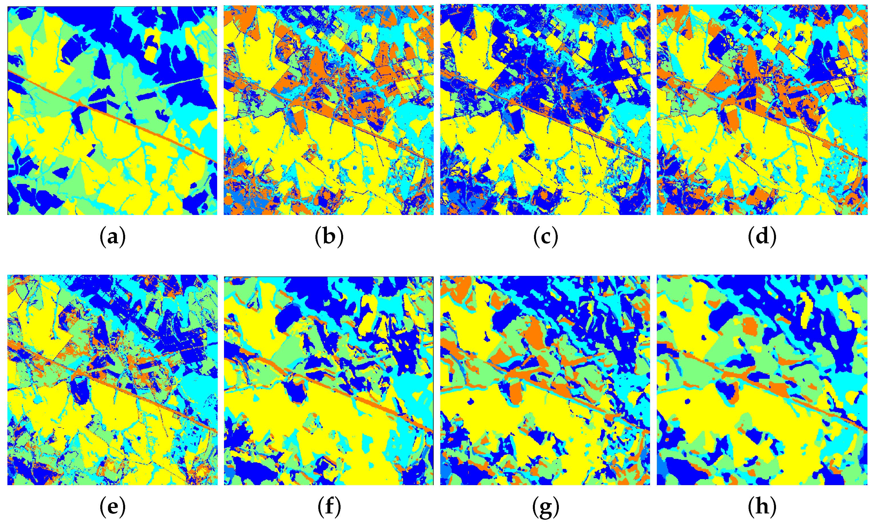
Figure 9.
Ground truth map and classification maps of the Landsat 5 TM multispectral image with (a) ground truth, (b) SVM, (c) Laplacian SVM, (d) SL SVM, (e) SL-Gabor SVM, (f) CNN-AE, (g) Supervised, (h) SLE-CNN.
Figure 9.
Ground truth map and classification maps of the Landsat 5 TM multispectral image with (a) ground truth, (b) SVM, (c) Laplacian SVM, (d) SL SVM, (e) SL-Gabor SVM, (f) CNN-AE, (g) Supervised, (h) SLE-CNN.

Figure 10.
Ground truth map and classification maps of the EMISAR image with (a) ground truth, (b) SVM, (c) Laplacian SVM, (d) SL SVM, (e) SL-Gabor SVM, (f) CNN-AE, (g) Supervised, (h) SLE-CNN.
Figure 10.
Ground truth map and classification maps of the EMISAR image with (a) ground truth, (b) SVM, (c) Laplacian SVM, (d) SL SVM, (e) SL-Gabor SVM, (f) CNN-AE, (g) Supervised, (h) SLE-CNN.

Figure 11.
Classification accuracies of the designed layer-wise embedding CNN with totally random sampling strategy and superpixel-based random sampling strategy in (a) HSI data, (b) MSI data, (c) SAR data.
Figure 11.
Classification accuracies of the designed layer-wise embedding CNN with totally random sampling strategy and superpixel-based random sampling strategy in (a) HSI data, (b) MSI data, (c) SAR data.

Figure 12.
The impact of the number of labeled training samples per class on the OA in (a) HSI data, (b) MSI data, (c) SAR data.
Figure 12.
The impact of the number of labeled training samples per class on the OA in (a) HSI data, (b) MSI data, (c) SAR data.


Table 1.
Number of samples (NoS) and colors of each class in the ground truth of the ROSIS Pavia University hyperspectral image.
Table 1.
Number of samples (NoS) and colors of each class in the ground truth of the ROSIS Pavia University hyperspectral image.
| Class | Name | NoS | Class | Name | NoS |
|---|---|---|---|---|---|
| 1 | asphalt | 6631 | 6 | bare soil | 5029 |
| 2 | meadows | 18,649 | 7 | bitumen | 1330 |
| 3 | gravel | 2099 | 8 | bricks | 3682 |
| 4 | trees | 3064 | 9 | shadows | 947 |
| 5 | metal sheets | 1345 | Total | 42,776 | |
Table 2.
Number of samples (NoS) and colors of each class in the ground truth of the Landsat 5 TM multispectral image.
Table 2.
Number of samples (NoS) and colors of each class in the ground truth of the Landsat 5 TM multispectral image.
| Class | Name | NoS |
|---|---|---|
| 1 | cultures | 62,322 |
| 2 | dams | 464 |
| 3 | bushes | 47,985 |
| 4 | grass lands | 59,883 |
| 5 | reforesting | 85,189 |
| 6 | roads | 2937 |
| Total | 258,780 | |
Table 3.
Number of samples (NoS) and colors of each class in the ground truth of the EMISAR image.
| Class | Name | NoS |
|---|---|---|
| 1 | winter wheat | 1088 |
| 2 | coniferous | 12,851 |
| 3 | water | 6695 |
| 4 | oat | 1172 |
| 5 | rye | 1767 |
| Total | 23,573 | |
Table 4.
Parameter settings in each layer of the layer-wise embedding CNN.
| Setting | Encoder/Decoder Layer | |||
|---|---|---|---|---|
| 1st | 2nd | 3rd | 4th | |
| Filter size | ||||
| Number of filters | 3 | 6 | 6 | 9 |
| Pooling stride | [2 2] | [2 2] | [2 2] | [2 2] |
| Padding type | SAME | SAME | SAME | SAME |
| Activation function | ReLU | ReLU | ReLU | ReLU |
| Denoising cost | 100 | 10 | 1 | 0.1 |
Table 5.
OA [%], AA [%], Kappa [%] and F-Measure [%] results for the HSI data with 5 labeled samples per class.
Table 5.
OA [%], AA [%], Kappa [%] and F-Measure [%] results for the HSI data with 5 labeled samples per class.
| Class | SVM | LapSVM | SL SVM | SL-Gabor SVM | CNN-AE | Supervised | SLE-CNN |
|---|---|---|---|---|---|---|---|
| asphalt a | 74.64 ± 0.15 | 78.24 ± 0.21 | 78.37 ± 0.12 | 80.23 ± 0.21 | 77.95 ± 0.13 | 71.36 ± 0.15 | 80.20 ± 0.12 |
| meadows | 61.69 ± 0.24 | 65.18 ± 0.14 | 63.14 ± 0.15 | 62.54 ± 0.30 | 77.84 ± 0.15 | 66.55 ± 0.27 | 79.16 ± 0.14 |
| gravel | 42.12 ± 0.32 | 40.16 ± 0.32 | 48.96 ± 0.37 | 50.91 ± 0.45 | 58.21 ± 0.32 | 37.59 ± 0.42 | 60.33 ± 0.22 |
| trees | 51.33 ± 0.33 | 64.15 ± 0.10 | 56.82 ± 0.23 | 64.25 ± 0.24 | 68.43 ± 0.18 | 62.71 ± 0.33 | 84.56 ± 0.11 |
| metal sheets | 56.31 ± 0.16 | 92.76 ± 0.08 | 77.57 ± 0.12 | 85.18 ± 0.13 | 95.15 ± 0.04 | 95.67 ± 0.02 | 97.11 ± 0.08 |
| bare soil | 34.85 ± 0.29 | 40.39 ± 0.27 | 39.10 ± 0.38 | 41.36 ± 0.37 | 55.63 ± 0.27 | 57.83 ± 0.27 | 60.57 ± 0.25 |
| bitumen | 66.92 ± 0.37 | 54.28 ± 0.16 | 60.29 ± 0.24 | 62.57 ± 0.23 | 56.44 ± 0.33 | 50.22 ± 0.26 | 55.89 ± 0.32 |
| bricks | 61.77 ± 0.12 | 66.92 ± 0.15 | 64.04 ± 0.22 | 63.60 ± 0.21 | 67.29 ± 0.16 | 63.64 ± 0.21 | 70.58 ± 0.17 |
| shadows | 98.48 ± 0.04 | 98.33 ± 0.05 | 99.63 ± 0.06 | 98.53 ± 0.05 | 96.45 ± 0.02 | 99.45 ± 0.04 | 97.31 ± 0.03 |
| OA | 60.62 ± 0.29 | 65.33 ± 0.27 | 63.29 ± 0.29 | 66.55 ± 0.31 | 72.36 ± 0.14 | 66.56 ± 0.29 | 75.49 ± 0.20 |
| AA | 65.08 ± 0.20 | 69.97 ± 0.22 | 69.39 ± 0.27 | 70.93 ± 0.18 | 74.44 ± 0.15 | 70.09 ± 0.28 | 76.99 ± 0.19 |
| Kappa | 49.83 ± 0.18 | 57.08 ± 0.19 | 54.66 ± 0.28 | 59.44 ± 0.30 | 66.30 ± 0.20 | 65.80 ± 0.23 | 68.83 ± 0.26 |
| F-Measure | 60.90 ± 0.24 | 66.71 ± 0.27 | 65.32 ± 0.19 | 67.69 ± 0.23 | 72.60 ± 0.17 | 67.22 ± 0.15 | 76.19 ± 0.16 |
a Lines 2 to 10 are the F-Measure per class.
Table 6.
OA [%], AA [%], Kappa [%] and F-Measure [%] results for the MSI data with 5 labeled samples per class.
Table 6.
OA [%], AA [%], Kappa [%] and F-Measure [%] results for the MSI data with 5 labeled samples per class.
| Class | SVM | LapSVM | SL SVM | SL-Gabor SVM | CNN-AE | Supervised | SLE-CNN |
|---|---|---|---|---|---|---|---|
| cultures a | 48.86 ± 0.32 | 46.89 ± 0.26 | 45.37 ± 0.28 | 42.44 ± 0.34 | 69.31 ± 0.25 | 53.65 ± 0.32 | 71.98 ± 0.15 |
| dams | 30.56 ± 0.45 | 33.90 ± 0.41 | 34.52 ± 0.42 | 36.66 ± 0.42 | 41.02 ± 0.37 | 38.27 ± 0.55 | 46.51 ± 0.40 |
| bushes | 67.23 ± 0.26 | 70.31 ± 0.19 | 68.51 ± 0.17 | 70.53 ± 0.27 | 52.36 ± 0.34 | 48.55 ± 0.30 | 50.17 ± 0.37 |
| grass lands | 42.18 ± 0.39 | 46.11 ± 0.45 | 44.72 ± 0.34 | 51.29 ± 0.32 | 45.34 ± 0.41 | 43.16 ± 0.44 | 45.95 ± 0.45 |
| reforesting | 80.35 ± 0.13 | 84.09 ± 0.08 | 82.94 ± 0.16 | 86.10 ± 0.15 | 84.89 ± 0.16 | 85.48 ± 0.18 | 86.39 ± 0.18 |
| roads | 58.25 ± 0.32 | 63.47 ± 0.32 | 59.45 ± 0.35 | 65.28 ± 0.25 | 66.53 ± 0.28 | 63.99 ± 0.26 | 67.42 ± 0.28 |
| OA | 53.20 ± 0.28 | 58.58 ± 0.34 | 56.26 ± 0.29 | 58.76 ± 0.26 | 59.08 ± 0.30 | 55.42 ± 0.32 | 60.96 ± 0.20 |
| AA | 50.92 ± 0.42 | 57.92 ± 0.23 | 56.27 ± 0.23 | 57.94 ± 0.34 | 60.33 ± 0.29 | 61.29 ± 0.22 | 62.67 ± 0.29 |
| Kappa | 45.30 ± 0.30 | 46.37 ± 0.33 | 46.56 ± 0.31 | 47.60 ± 0.35 | 48.84 ± 0.31 | 46.26 ± 0.44 | 50.47 ± 0.36 |
| F-Measure | 54.57 ± 0.31 | 57.46 ± 0.29 | 55.92 ± 0.31 | 58.72 ± 0.29 | 59.91 ± 0.27 | 55.52 ± 0.34 | 61.40 ± 0.26 |
a Lines 2 to 7 are the F-Measure per class.
Table 7.
OA [%], AA [%], Kappa [%] and F-Measure [%] results for the SAR data with 5 labeled samples per class.
Table 7.
OA [%], AA [%], Kappa [%] and F-Measure [%] results for the SAR data with 5 labeled samples per class.
| Class | SVM | LapSVM | SL SVM | SL-Gabor SVM | CNN-AE | Supervised | SLE-CNN |
|---|---|---|---|---|---|---|---|
| winter wheat a | 48.52 ± 0.43 | 57.11 ± 0.31 | 54.17 ± 0.40 | 61.26 ± 0.34 | 94.47 ± 0.09 | 84.73 ± 0.15 | 93.16 ± 0.05 |
| coniferous | 96.31 ± 0.02 | 97.48 ± 0.05 | 98.30 ± 0.02 | 98.41 ± 0.06 | 98.24 ± 0.05 | 98.95 ± 0.03 | 98.97 ± 0.04 |
| water | 80.47 ± 0.11 | 88.14 ± 0.16 | 87.26 ± 0.16 | 89.18 ± 0.11 | 90.43 ± 0.02 | 92.15 ± 0.08 | 91.49 ± 0.08 |
| oat | 69.50 ± 0.25 | 83.37 ± 0.13 | 80.19 ± 0.18 | 79.67 ± 0.16 | 91.15 ± 0.11 | 80.49 ± 0.16 | 94.38 ± 0.05 |
| rye | 72.93 ± 0.16 | 86.32 ± 0.18 | 84.58 ± 0.13 | 87.52 ± 0.19 | 92.68 ± 0.08 | 89.17 ± 0.13 | 96.33 ± 0.08 |
| OA | 74.19 ± 0.18 | 84.36 ± 0.14 | 82.37 ± 0.07 | 85.20 ± 0.15 | 93.41 ± 0.09 | 91.08 ± 0.11 | 95.74 ± 0.08 |
| AA | 66.38 ± 0.19 | 75.66 ± 0.22 | 73.49 ± 0.24 | 76.97 ± 0.17 | 90.50 ± 0.06 | 84.29 ± 0.18 | 92.90 ± 0.07 |
| Kappa | 60.30 ± 0.22 | 75.03 ± 0.13 | 72.18 ± 0.25 | 76.89 ± 0.23 | 89.10 ± 0.14 | 89.20 ± 0.13 | 90.07 ± 0.11 |
| F-Measure | 73.55 ± 0.14 | 82.48 ± 0.17 | 80.90 ± 0.19 | 83.21 ± 0.13 | 93.39 ± 0.07 | 89.10 ± 0.17 | 94.87 ± 0.12 |
a Lines 2 to 6 are the F-Measure per class.
© 2019 by the authors. Licensee MDPI, Basel, Switzerland. This article is an open access article distributed under the terms and conditions of the Creative Commons Attribution (CC BY) license (http://creativecommons.org/licenses/by/4.0/).
Share and Cite
MDPI and ACS Style
Liu, H.; Li, J.; He, L.; Wang, Y. Superpixel-Guided Layer-Wise Embedding CNN for Remote Sensing Image Classification. Remote Sens. 2019, 11, 174. https://0-doi-org.brum.beds.ac.uk/10.3390/rs11020174
AMA Style
Liu H, Li J, He L, Wang Y. Superpixel-Guided Layer-Wise Embedding CNN for Remote Sensing Image Classification. Remote Sensing. 2019; 11(2):174. https://0-doi-org.brum.beds.ac.uk/10.3390/rs11020174
Chicago/Turabian StyleLiu, Han, Jun Li, Lin He, and Yu Wang. 2019. "Superpixel-Guided Layer-Wise Embedding CNN for Remote Sensing Image Classification" Remote Sensing 11, no. 2: 174. https://0-doi-org.brum.beds.ac.uk/10.3390/rs11020174
Note that from the first issue of 2016, this journal uses article numbers instead of page numbers. See further details here.