Reconstructing Geostationary Satellite Land Surface Temperature Imagery Based on a Multiscale Feature Connected Convolutional Neural Network

Abstract

Geostationary satellite land surface temperature (GLST) data are important for various dynamic environmental and natural resource applications for terrestrial ecosystems. Due to clouds, shadows, and other atmospheric conditions, the derived LSTs are often missing a large number of values. Reconstructing the missing values is essential for improving the usability of the geostationary satellite LST data. However, current reconstruction methods mainly aim to fill the values of a small number of invalid pixels with many valid pixels, which can provide useful land surface temperature values. When the missing data extent becomes large, the reconstruction effect will worsen because the relationship between different spatiotemporal geostationary satellite LSTs is complex and highly nonlinear. Inspired by the superiority of the deep convolutional neural network (CNN) in solving highly nonlinear and dynamic problems, a multiscale feature connection CNN model is proposed to fill missing LSTs with large missing regions. The proposed method has been tested on both FengYun-2G and Meteosat Second Generation-Spinning Enhanced Visible and InfraRed Imager geostationary satellite LST datasets. The results of simulated and actual experiments show that the proposed method is accurate to within about 1 °C, with 70% missing data rates. This is feasible and effective for large regions of LST reconstruction tasks.

1. Introduction

As an important variable of the weather and climate system, land surface temperature (LST) has been widely used for a variety of purposes, including meteorological, hydrological, and ecological research; urban heat island monitoring; and so on [1,2]. Due to advances in satellite remote sensing, global LST datasets, which are more attractive than traditional in situ regional measurements, have become available [3,4]. Given their high temporal resolution, LSTs acquired from geostationary satellites can build detailed representations of diurnal temperature cycles [5]. Accordingly, near-real time environment monitoring can be achieved, including estimating surface energy budget and crop growth or monitoring volcanic activity and fires [6]. Like other satellite remote sensing data, there are usually a number of invalid values in LSTs determined by geostationary satellites on account of sensor malfunction and poor atmospheric conditions. This has a strong impact on the subsequent usage rate. Therefore, reconstructing geostationary satellite LST data is of considerable importance [7].

To date, several methods have been developed and applied to reconstruct the missing values in remotely sensed LSTs [8,9,10,11]. Most of these approaches can be classified into three categories: (1) spatial information-based methods [7,12,13], (2) multi-temporal information-based methods [9,14,15,16], and (3) spatiotemporal information-based methods [17,18,19]. The spatial reconstruction methods mainly use the valid pixels around the missing data pixel to recover the invalid data based on pixel-disaggregating, inverse distance weighting (IDW), spline function, and cokriging interpolation algorithms. These methods are easy to realize and perform well when in homogeneous landscapes with a small extent of invalid values. Temporal reconstruction methods use the complementary temporal images of the same regions at adjacent times to recover the missing pixels, and the algorithms employed primarily include the linear temporal approach, the harmonic analysis method, the temporal Fourier analysis approach, asymmetric Gaussian function fitting method, and the diurnal temperature cycle (DTC)-based method. As stated above, geostationary satellite LSTs can fully reveal the diurnal change in LSTs; hence, the DTC-based method is usually applied to reconstruct geostationary satellite LST data. Though these time-domain approaches perform well for filling missing LSTs, they lose efficacy when there is insufficient valid data to calculate the model parameters. In addition, selecting the proper model to represent the DTC is difficult, and acquiring the best solution using these methods is usually complicated. In view of the unsatisfactory results derived from spatial information-based methods or temporal information-based methods, some spatiotemporal information-based LST reconstruction methods have been proposed. For instance, Liu et al. [18] presented a spatiotemporal reconstruction method for Feng Yun-2F (FY-2F) LST missing data. Simulated and real data experiments indicated that the method can work well, with the root mean square error (RMSE) within about 2 °C in most cases [18]. Weiss et al. [19] proposed a gap-filling approach for LST image time-series data using both neighboring (non-gap) data and data from other time periods (i.e., calendar date or multi-year datasets). However, these methods do not consider temporal and spatial information simultaneously or do not give enough consideration. More importantly, they need enough data points and considerable manual intervention. Finally, all three of the above approaches perform poorly if the region to be reconstructed is large. A major reason for this is that these methods fail to learn high dynamic spatiotemporal relationships of LSTs with limited useful information.

In recent years, convolutional neural networks (CNNs) have been increasingly employed in remote sensing data processing tasks [20,21]. They have the ability to automatically learn inherent complex relationships between different data [22]. For cloud-contaminated, remotely-sensed information reconstruction, Malek et al. [23] used a contextualized auto-encoder CNN model to reconstruct cloud-contaminated remote sensing images at a pixel and a patch level, and Zhang et al. [24] proposed a unified deep CNN to recover missing data in remote sensing images under three conditions. Both perform well when the neighborhoods of the missing areas are representative enough. Moreover, unlike LST, the surface reflectance or digital number (DN) varies gradually as time changes. As a result, these models are not suitable for reconstructing LSTs with high spatiotemporal dynamics for large missing regions.

This article describes how a multiscale feature connection GLST reconstruction CNN (MFCTR-CNN) was developed for LST images with large missing regions. The main contributions can be summarized as follows: (1) A CNN-based model is introduced to reconstruct missing GLSTs with large regions. It can automatically learn the highly dynamic GLST spatiotemporal relationship, which is important for the recovery task. Additionally, when the model is well trained, it can be used directly without any manual intervention. Therefore, it can perform mass reconstruction of LSTs. (2) To fully use the complementary temporal data, two inputs are added and concatenated. As such, the spatial and temporal information is combined together in an image. (3) Low- and high-level information at different scales with spatial attention units are connected in the model, so the useful multilevel information of the input data can be fully utilized to better recover detailed features and spatial information, considerably improving the performance of the MFCTR-CNN.

The remainder of this article is arranged as follows. The architecture of the reconstruction model is described in Section 2. In Section 3, we first introduce the data sets and settings used in the experiments, then provide the results of the experiments. Discussion about this proposed work is described in Section 4. Finally, the conclusions are provided in Section 5.

2. Reconstruction Architecture

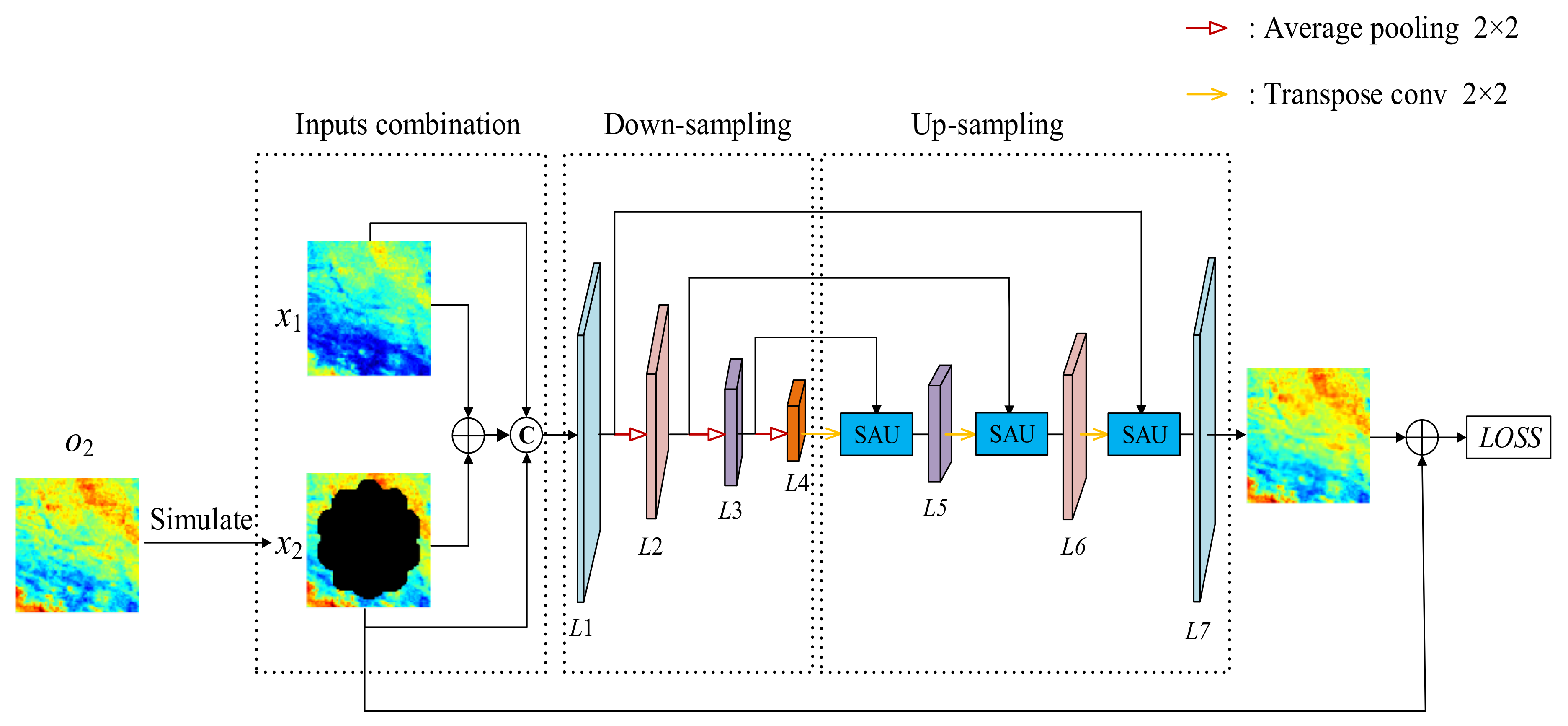
The proposed reconstruction model is a Multiscale Feature Connected Fully Convolutional Neural Network. The network adopts an encoder–decoder architecture that is suitable for many image processing tasks. The detailed structure is depicted in Figure 1. The MFCTR-CNN mainly includes three components: (1) multi-temporal data combination, (2) a down-sampling procedure, and (3) up-sampling and a spatial attention unit (SAU). Detailed descriptions of each component are outlined below.

2.1. Temporal Data Combination

It has been proven that complementary data are useful for remote sensing data reconstruction [23]. Thus, for the missing GLST recovery, the proposed MFCTR-CNN has two types of inputs: the GLST image at time t2 with missing regions (input x₂ in Figure 1) and the auxiliary GLST image without invalid pixels at time t1 (input x₁ in Figure 1).

In order to better utilize both inputs, input x₁ and x₂ are first added. As such, we can preferably take advantage of the high spatial information of the two inputs. Then, we composite x₁, x₂, and the added results. This fully unites the information of GLSTs at different times, so the high temporal dynamic relationship between GLSTs will be used well. As a result, the spatiotemporal information can be utilized simultaneously in our model.

2.2. Features of GLST Extraction by the Down-Sampling Procedure

Deep neural networks make use of the fact that plenty of natural signals are compositional hierarchies, in which lower level features can form higher level ones [20]. Inspired by this, we first extracted the internal and underlying features of the output, which were derived in Section 2.1 using the down-sampling procedure, to learn about the high spatiotemporal relationship between GLSTs. The down-sampling part of the MFCTR-CNN involves stacked convolution layers and pooling layers. A detailed description is shown in

Table 1. Convolution layers of the multiscale feature connection GLST reconstruction CNN (MFCTR-CNN).

Down-Sampling			Up-Sampling
Level	Layer	Size		Layer	Level
L1	{conv 3 × 3, 64, batch normalization} × 2	1	1	{conv 3 × 3, 64, batch normalization} × 2 conv 3 × 3, 32, batch normalization conv 3 × 3, 1	L7
L2	{conv 3 × 3, 128, batch normalization} × 2	1/2	1/2	{conv 3 × 3, 128, batch normalization} × 2	L6
L3	{conv 3 × 3, 256, batch normalization} × 2	1/4	1/4	{conv 3 × 3, 256, batch normalization} × 2	L5
L4	{conv 3 × 3, 512, batch normalization} × 2	1/8

. Convolution is usually utilized to obtain features of the input data, such as extracting edges of objects. A convolution layer takes an image patch and filter kernels as its input and exports the high-level feature map of the input image. The high-level feature map can be denoted as

$$Y_l=W_l{X}_l+b_l$$

(1)

where Y_l represents the output feature map, W_l and b_l are the parameters of the convolution filter, and X_l denotes the input feature maps.

In the training process of CNNs, even small variations in the previous layers are amplified through the network. Therefore, the probability distribution of the layers’ output does not coincide with that of the layers’ input, which causes defects such as slow convergence rate and overfitting of model parameters. This consequently affects the reconstruction results. To solve this problem, a batch normalization layer was added behind the convolution layer in the proposed MFCTR-CNN. Batch normalization introduces two extra parameters to transform and reconstitute the normalization result of the convolution layer’s output. For the purpose of determining the high spatiotemporal dynamic nonlinear relationship between different GLSTs, we ensured that the output of the CNN was a nonlinear combination of the input. Hence, a rectified linear unit (ReLU) [25] activation layer (max (0, ·)) was adopted after convolution, and batch normalization layers for nonlinearity were produced in the network.

In order to fill missing GLSTs with large regions, relationships among different pixels with a large range had to be built. Therefore, it was necessary to extend the receptive field during convolution to enhance the contextual information of feature maps of GLST. Usually, there are three methods to achieve this aim: (1) amplifying the convolution kernel filter size, (2) using dilated convolution layers, and (3) employing pooling layers. However, amplifying the convolution kernel filter size will greatly increase the number of convolution parameters of the CNN, thereby requiring considerable computer GPU memory and time to calculate and train. A dilated convolution layer can expand the receptive field and maintain the convolution kernel filter size concurrently. However, on one hand, it needs to carry out convolution on a large number of high resolution feature maps, so the demands in terms of computer GPU memory and time to train the model are high. On the other hand, dilated convolution may cause important information to be missed because of the rough sub-sampling. In the proposed MFCTR-CNN, we used average pooling layers to better enlarge the receptive field. Average pooling further extracts the feature maps and retains the background information without any extra parameters. However fine features and precise spatial information of GLSTs will be lost in the pooling process. To overcome this problem, feature maps of the same scales in the down-sampling and up-sampling processes are connected in MFCTR-CNN. Using this process, the localization accuracy discarded by the up-sampling procedure is reserved, while the context information of GLSTs is preserved.

After the down-sampling procedure, the spatial information, temporal information, and latent correlation of input image patch/es are extracted synchronously, and all of them are stored in the generated high-level LST feature maps, which is key to reconstruct invalid values.

2.3. GLST Image Recovery Using Up-Sampling and a Spatial Attention Unit

To reconstruct the missing GLSTs, the high-level feature maps extracted in Section 2.2 were gradually recovered to the size that was the same as the input. Transpose convolution was used in MFCTR-CNN to realize the size-recovery target. Transpose convolution is the inverse process of convolution that can enlarge the size of input feature maps according to demand. As shown in Figure 1, the size of the feature maps in the up-sampling process was gradually resized to the same size of the feature maps in the down-sampling procedure.

As mentioned above, the positional information of GLST pixels will be lost in the down-sampling procedure. However, low-level GLST features in the down-sampling can be utilized to overcome this problem. Skip connection structure, which concatenates the low-level features and high-level features directly, is generally applied to realize the reuse of positional information [26]. However, restoring pixels’ locational information usually does not require all the information in the low-level features. Meanwhile, overall feature concatenation will give rise to the over-use of low-level information and finally lead to over-fitting [27]. Illuminated by the phenomenon that many animals concentrate on specific parts of their visual objects to make adequate responses, an attention mechanism was put forward to choose the most pertinent low-level feature information in deep learning, and it has been widely adopted in image processing tasks, such as classification [28], segmentation [29], object recognition [30], and other aspects [31,32,33,34,35,36]. 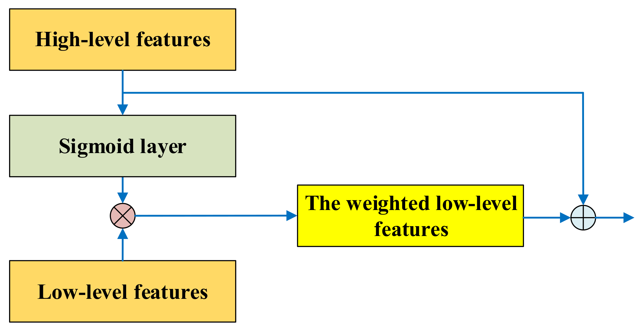In this article, a spatial attention unit (SAU) is added to the proposed network, the architecture of which is depicted in Figure 2. With the help of high-level features and the sigmoid layer, a spatial attention unit can automatically heighten useful low-level features and weaken unnecessary low-level information of GLST. In the spatial attention unit, the high-level features are firstly fed into a sigmoid layer. This layer can output the weights of low-level features by activating useful information of relevant high-level features. Then, the low-level features are multiplied by the output of the sigmoid layer to attain the weighted low-level features. Lastly, the high-level features and the weighted low-level features are added as the input of convolution layers in the up-sampling procedure.

Beside transpose convolution and the spatial attention unit, a two-layer convolution layer, which is the same as in the down-sampling procedure, is also added to the network. Their elaborate structure is described in Table 1. In the final convolution layer, the previous feature maps were aggregated to a single channel image with the same size of the input by using a 3 × 3 convolution, which can convert high-level information into the output. Because the output results are the same as the input values in intact areas, a residual learning strategy was applied in the proposed model. The loss of the network is represented as

$$L(\Theta )=\frac{1}{2N}{\displaystyle \sum _{i=1}^N{\Vert F\left(x_1,x_2;\Theta \right)-\left(o_2-x_2\right)\Vert }^2}$$

(2)

where L(Θ) is the loss of training data, Θ are the network parameters (including weights and biases), N denotes the number of missing values, and O₂ is the real data of the missing regions. After finishing error forward propagation, a back-propagation algorithm was used to update parameters to better learn the relationship among LSTs.

3. Experiments

In this section, the effectiveness of the proposed reconstruction MFCTR-CNN is verified. A comparison between the proposed MFCTR-CNN and some traditional reconstruction methods should be given. Theoretically, the spatiotemporal reconstruction method is an optimal choice, such as that described in references [19,18]. However, the choice of spatial information or temporal information requires considerable manual intervention, which makes these methods vastly uncontrollable. Recently, Pede and Mountrakis compared different interpolation methods for LST reconstruction [37] and provided strong evidence that spatial and spatiotemporal methods have greater predictive capabilities than temporal methods, regardless of the time of day or season. To minimize manual intervention, the spatial information-based method was selected. Here the spline spatial interpolation method is recommended based on the following: (1) The performance of the spline spatial method is no worse than that of the spatiotemporal method when the LST image has cloud cover of <80% [37]. (2) Spline functions are readily available and easy to implement through several software packages [37]. (3) There is no need for auxiliary data from other stated time periods (i.e., the same season or multi-year datasets), which is similar to the proposed method. To contribute to the geoscience community, the implementation code, the trained network and the testing dataset were released in open-source format and can be publicly accessed via GitHub (https://github.com/ahuyzx/MFCTR-CNN).

3.1. Datasets

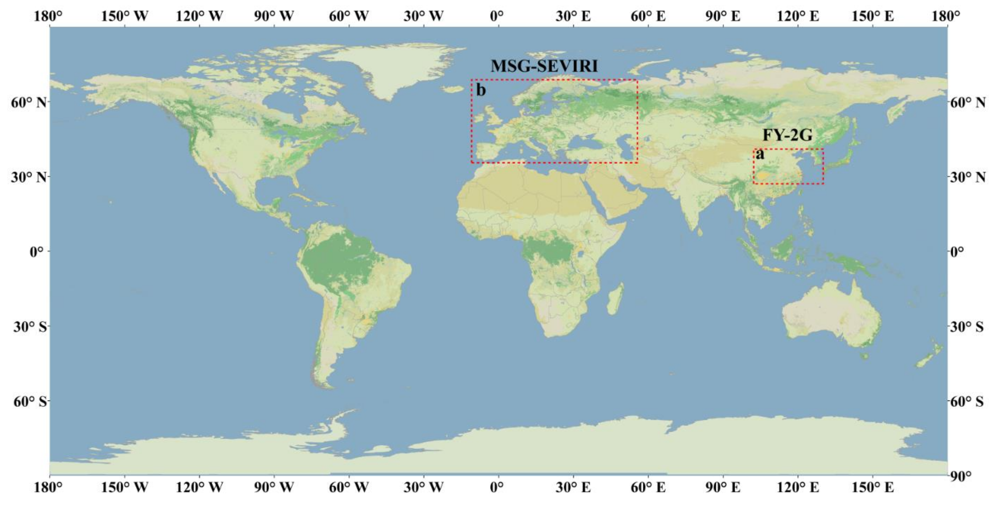
In order to evaluate the proposed reconstruction model, two kinds of publicly accessible GLST datasets from different sensors were used for the experiments. They are FengYun-2G (FY-2G LST; with a 5 km spatial resolution at nadir and 1 h temporal resolution) and the Meteosat Second Generation-Spinning Enhanced Visible and Infrared Imager geostationary satellite (MSG-SEVIRI) LST (with a 3 km spatial resolution at nadir and 15 min temporal resolution). For FY-2G LSTs, a subarea in of size 471 × 235 (as shown by the red dashed rectangle in Figure 3a) was selected as the study area. The land-cover types mainly are farmland, forestland, urban, and bare areas. For the MSG-SEVIRI LST, an area in Europe was selected as the experimental area. 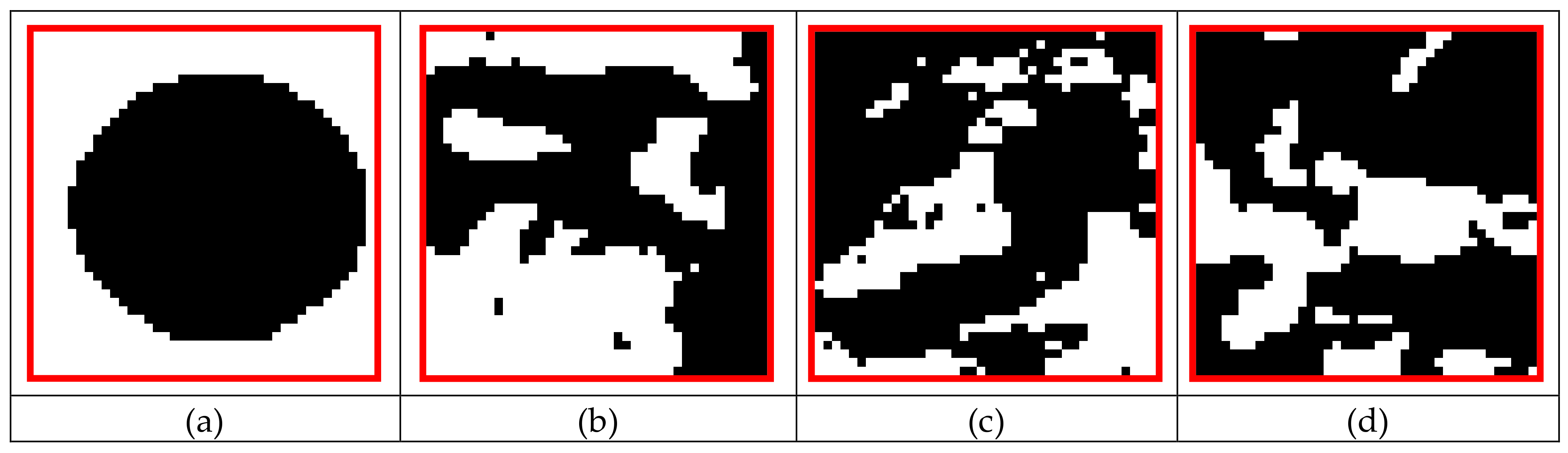Its imagery size is 1701 × 651 (as sketched using the red dashed rectangle in Figure 3b), and the main land-cover types in Europe are farmland, flooded vegetation, grass land, tree cover, urban, and bare areas. Both research areas contain multiple land-cover types, which can ensure the universality of the proposed method in sufficient land-cover conditions. Furthermore, experiments were conducted using LSTs from four seasons (i.e., spring, summer, autumn, and winter) for both FY-2G and MSG-SEVIRI LSTs. Specifically, FY-2G LST data used as training data sets were from July 2015, October 2015, January 2016, and April 2016, and MSG-SEVIRI LST data used were from July 2010, October 2010, January 2011, and April 2011. This allowed for testing of the performance of the proposed method in different climate conditions. All these data were arranged in sets of temporal pairs in chronological order with definite time intervals. Then, they were clipped into 40 × 40 patches, with 20 overlapping. The patches without an invalid value were selected as training datasets. To simulate different missing-pixel conditions, image masks were generated with varying pixel rates missing from true images without missing pixels. These masks were then added to clipped patches to produce images with different missing data rates (MDRs) and different distribution characteristics (DCs) of the missing observations (i.e., concentrated or scattered), as shown in Figure 4. The GLST data in the adjacent month of the same season were used to test the trained models. For example, FY-2G data in August 2015 were used as testing data for the trained model of July 2015. The testing data were clipped in the same way as the training data. In addition, LST images in the same month of the next year (i.e., FY-2G LST from July 2016 and MSG-SEVIRI LST from July 2011) were also selected as the testing data. Because LST varies largely in different periods within a day, the network was carried through in three time periods (i.e. 06:00–12:00, 12:00–18:00, and 18:00–06:00 local time) of a day, based on a previous study [18]. For convenience, the three time periods were tagged as S1, S2, and S3 in this study.

3.2. Network Training Details

Although networks with the ReLU activation layer are easier to train than the traditional sigmoid-like activation networks, it is hard for these networks to learn highly non-linear and dynamic systems when the weight parameters of the network are poorly initialized. Therefore, the robust weight initialization strategy introduced in He et al. [39] was adopted in the proposed model.

Because the Adam algorithm can adaptively update the weights of the network and can consequently achieve high efficiency in the training process, it was used as the gradient descent optimization method to train the proposed model. The learning rate (α) was initially set to 0.001 for the network. After every 30 epochs (the training process for both FY-2G LSTs and MSG-SEVIRI LSTs were all set to 60 epochs), α was multiplied by a decaying factor of 0.1 to decrease the searching range of the parameters. To prevent the overfitting of the network, L₂ regulation with a weight decay of 0.001 was applied to the model.

3.3. Experiment Results

In this section, we simulated initially contaminated GLST images with different MDRs (53, 65, and 70%) on undamaged clipped GLST image patches. The simulated contaminated GLST image patches were reconstructed using the proposed model and the classic spline spatial interpolation method, then assessed compared to the original GLST images with the RMSE index. In addition, for the actual experiments, FY-2G and SEVIRI LSTs with about 50% MDR were tested using the proposed MFCTR-CNN method.

3.3.1. Visual Performance of MFCTR-CNN in the Simulation Experiment

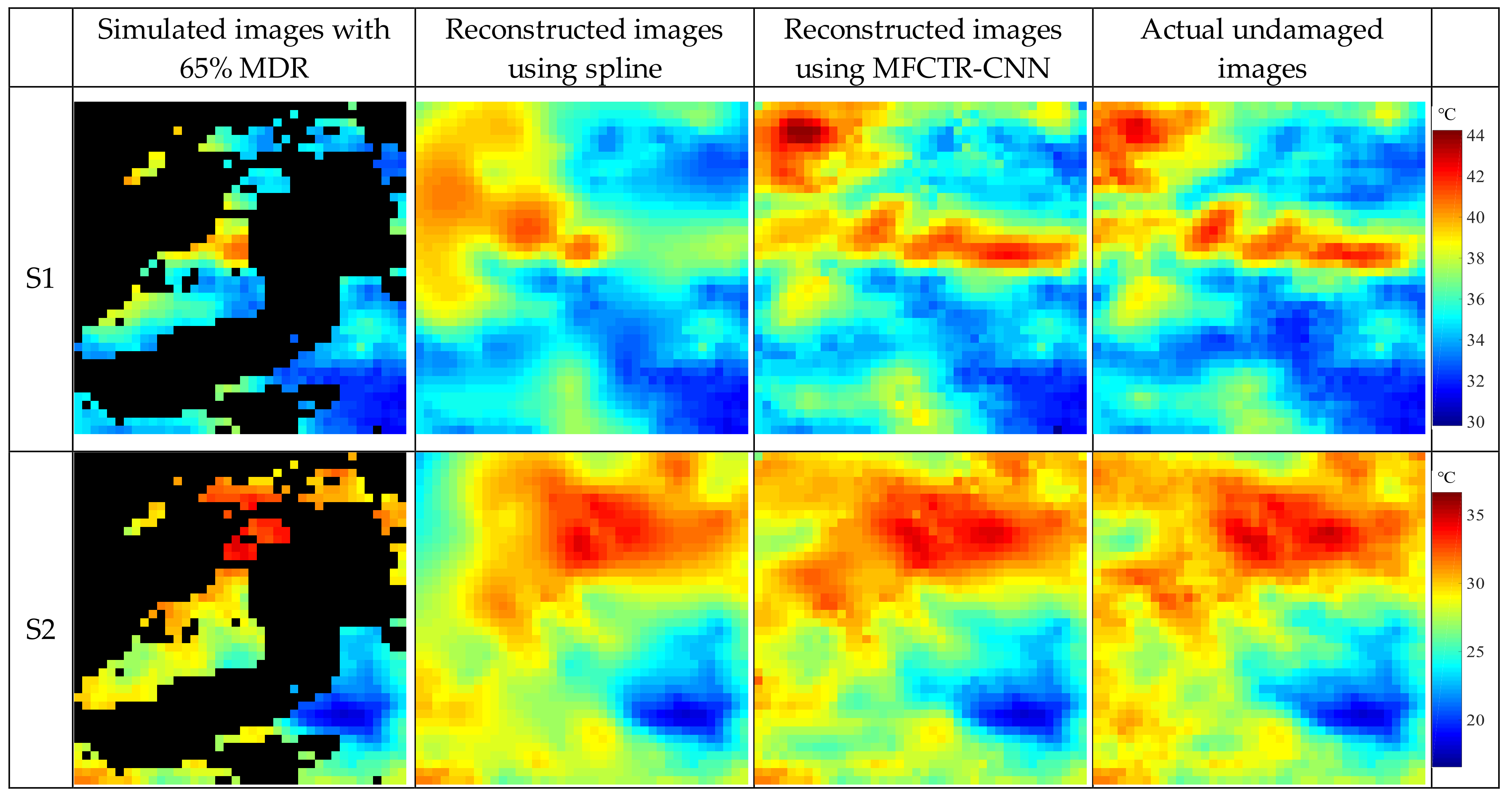
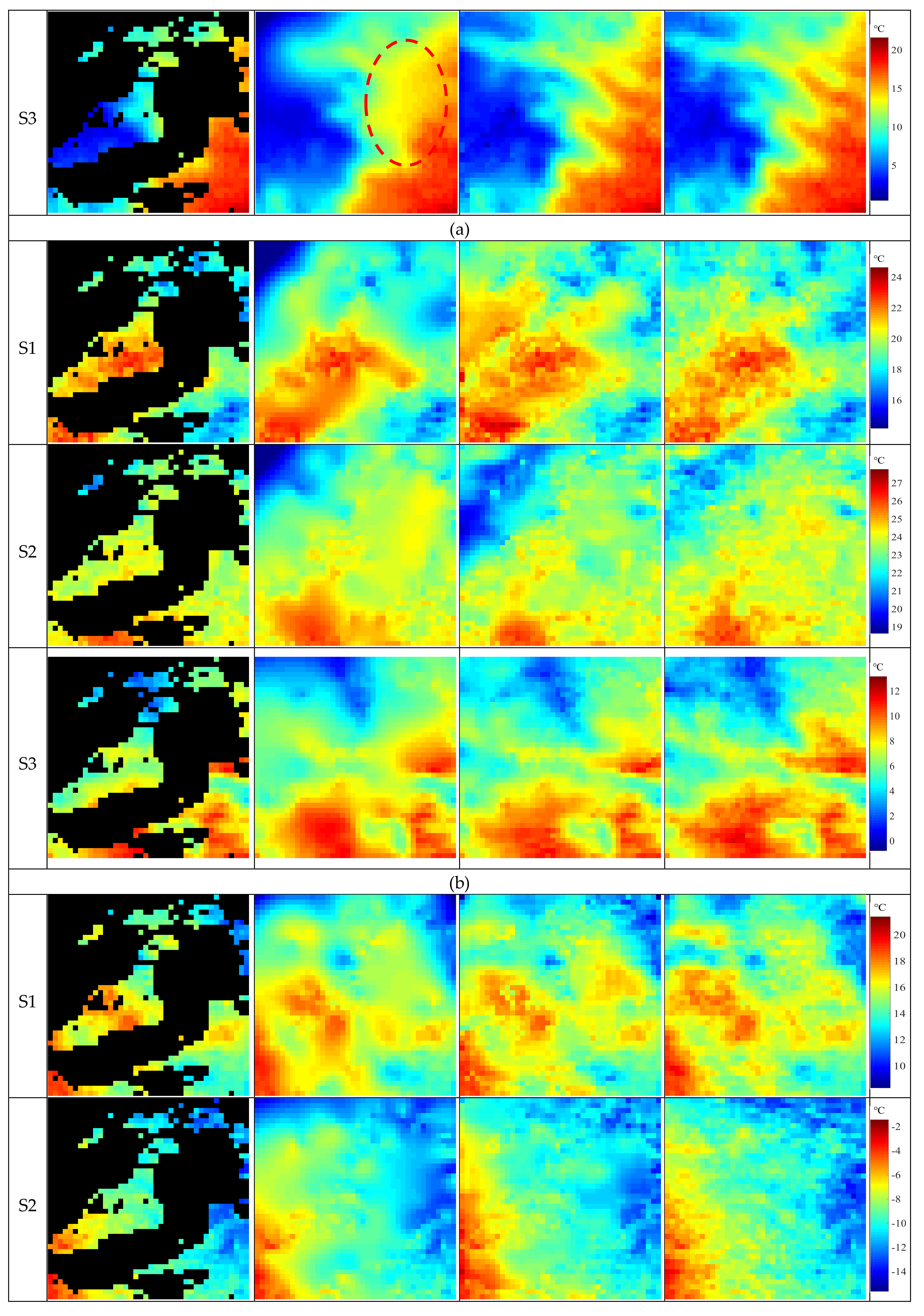
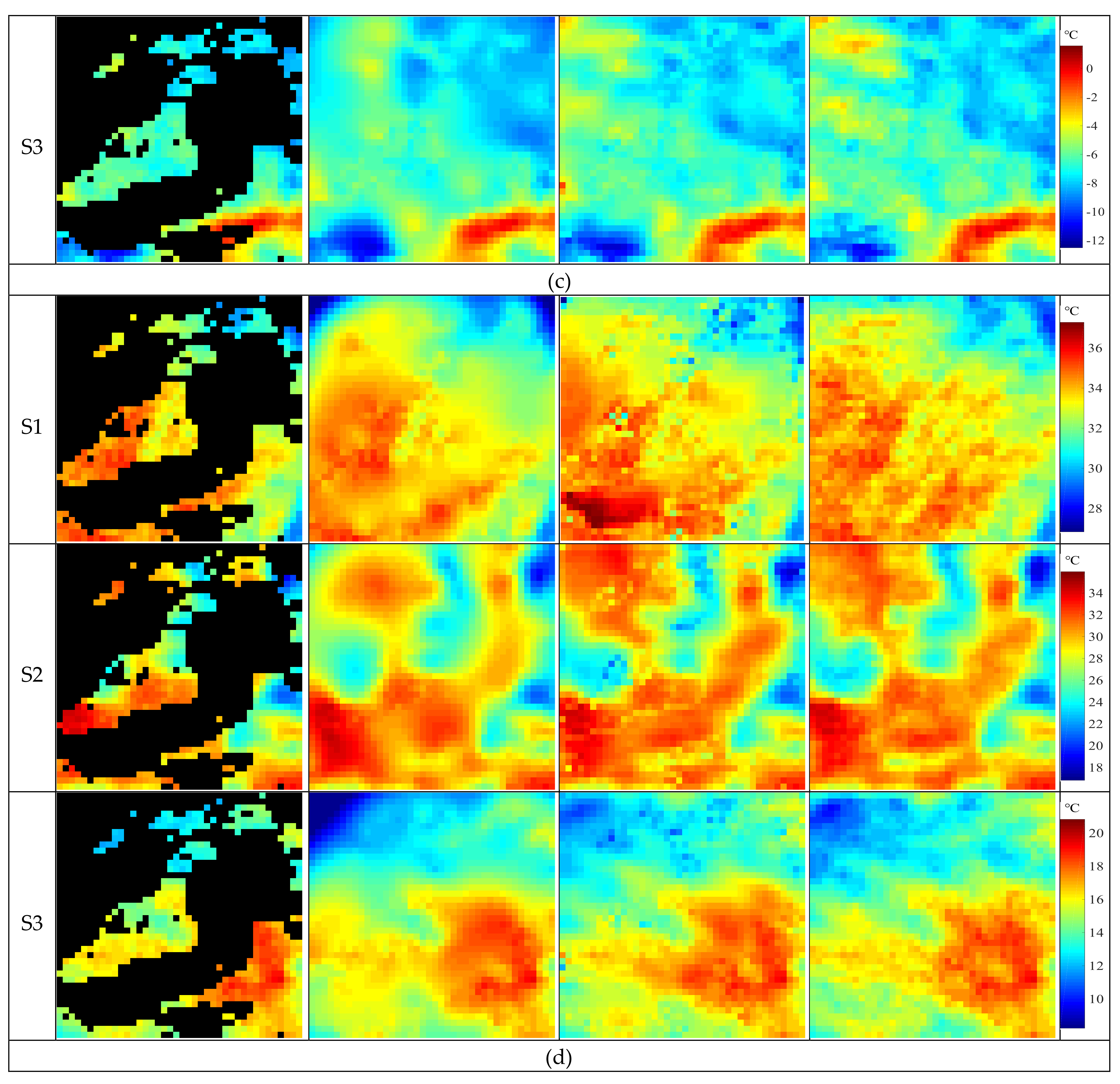
To compare the visual results of the proposed model and the classic spline spatial interpolation method (MFCTR-CNN versus spline), we took LST images with simulated 65% MDR as an example and depicted some reconstructed LST images for FY-2G in the S1, S2, and S3 periods in different seasons, as showed in Figure 5. Generally, the MFCTR-CNN method maintained the detail features of the GLTS images better and had a bigger structural similarity with the actual undamaged LST image. 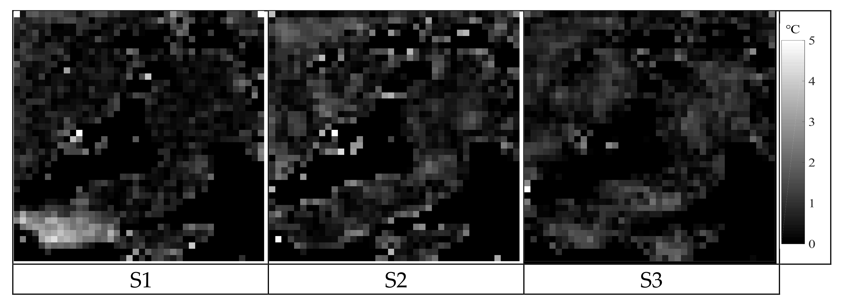Meanwhile, the spline method smoothed the results (one example was shown in the bold red dashed line of the S3 period in Figure 5a) and achieved blurry LST images. However, it is certain that LSTs are always varying highly dynamically both temporally and spatially. The MFCTR-CNN method is, therefore, more suitable for reconstructing LST images. Furthermore, it is evident that the results in the night time were better than those in the day when using the spline method, while the outcomes of MFCTR-CNN are nearly the same during both night and day. To better show the error distributions, examples of error maps from MFCTR-CNN for FY-2G LST images in May 2016 (spring) are shown in Figure 6. It can be seen that most errors are small and close with each other.

3.3.2. Quantitative Evaluation under Different MDRs and DCs

In order to compare the capabilities of the proposed method and the spline spatial interpolation method, the quantitative statistical results with RMSEs for the two methods with different MDRs (53%, 65% and 70%) and different DCs are listed in

Table 2. Error metrics comparison of the proposed MFCTR-CNN and spline method with different MDRs.

			RMSEs with Different MDR
			53% Concentrated		53% Scattered		65%		70%
			MFCTR-CNN	Spline	MFCTR-CNN	Spline	MFCTR-CNN	Spline	MFCTR-CNN	Spline
	Next Summer	201607-S1	0.98	1.24	0.88	0.99	1.02	1.07	0.97	1.13
		201607-S2	0.98	1.54	1.02	1.39	1.12	1.45	1.19	1.58
		201607-S3	0.82	1.05	0.70	0.82	0.76	0.90	0.78	0.92
FY-2G	Summer	201508-S1	0.95	1.37	0.88	1.05	1.05	1.14	0.96	1.17
		201508-S2	0.74	1.87	0.75	1.43	0.85	1.45	0.89	1.59
		201508-S3	0.81	1.10	0.67	0.84	0.76	0.89	0.76	0.94
	Fall	201511-S1	0.89	1.22	0.95	0.97	1.07	1.00	0.99	1.07
		201511-S2	0.85	1.22	0.89	1.00	1.02	1.05	0.95	1.08
		201511-S3	0.59	1.09	0.61	0.89	0.64	0.94	0.67	0.97
	Winter	201602-S1	0.97	1.44	0.95	1.16	0.98	1.24	0.99	1.30
		201602-S2	0.84	1.50	0.81	1.23	0.85	1.23	0.89	1.35
		201602-S3	0.82	1.44	0.81	1.15	0.84	1.21	0.84	1.29
	Spring	201605-S1	0.74	1.48	0.80	1.26	1.04	1.42	0.95	1.36
		201605-S2	0.68	1.78	0.83	1.47	0.93	1.55	0.85	1.65
		201605-S3	0.85	1.13	0.89	1.04	0.81	1.19	0.76	1.13
	Next Summer	201107-S1	0.91	2.50	1.02	2.25	0.92	2.06	0.95	2.26
		201107-S2	0.89	2.60	1.04	2.42	0.98	2.17	0.97	2.38
		201107-S3	0.75	1.84	1.13	1.72	0.89	1.57	0.79	1.74
MSG	Summer	201008-S1	0.86	2.38	0.87	2.06	0.87	1.99	0.90	2.20
		201008-S2	0.82	2.33	0.87	1.99	0.94	1.97	0.90	2.13
		201008-S3	0.69	1.75	0.99	1.57	0.81	1.60	0.73	1.71
	Fall	201011-S1	0.89	1.64	0.91	1.53	0.96	1.52	0.95	1.61
		201011-S2	0.79	1.75	0.87	1.60	0.83	1.58	0.85	1.72
		201011-S3	0.70	1.99	0.70	1.79	0.69	1.72	0.71	1.93
	Winter	201102-S1	0.79	1.60	0.93	1.43	0.92	1.42	0.91	1.52
		201102-S2	0.75	1.71	0.82	1.55	0.84	1.57	0.87	1.67
		201102-S3	0.73	1.89	0.75	1.63	0.77	1.59	0.75	1.72
	Spring	201105-S1	0.79	1.81	0.72	1.38	0.83	1.63	0.86	1.74
		201105-S2	0.62	1.85	0.57	1.43	0.68	1.64	0.75	1.77
		201105-S3	1.06	1.11	0.55	0.89	0.91	1.09	1.00	1.12

. In particular, RMSEs from 53% MDR with concentrated pixels and with scattered pixels (like Figure 4a,b) are also compared. From the table, we can see that (1) for both FY-2G and MSG-SEVIRI data, average RMSEs of reconstruction results in different seasons and different years with the proposed method are mostly under 0.8 °C. Meanwhile, with regards to the spline method, the average RMSEs are mainly about 1.1 °C for FY-2G, and 1.7 °C for MSG-SEVIRI. It is obvious that the average RMSEs of MSG-SEVIRI by using the spline method are larger than that of FY-2G. This is probably due to the fact that the land-cover types of the MSG-SEVIRI study area are more complex than those of FY-2G, but this factor does not affect our network’s performance. (2) For the spline method, the RMSEs in summer and winter were bigger than those in the fall and spring. This is probably caused by the characteristics of LSTs with highly dynamical changes and the variation difference of LSTs under different land types in the winter and summer. (3) In general, both methods produced smaller errors at night than in the daytime for both FY-2G and MSG-SEVIRI. (4) For the MFCTR-CNN method, the RMSEs do not change much with different MDRs and different DCs of the missing observations. For the spline spatial interpolation method, however, the effect of reconstruction is affected by the DCs of the missing observations and the different MDRs. The errors increase as the MDR changes from 53 to 70%. Furthermore, under the same MDR, if the distribution of the missing observations is relatively concentrated, the errors are bigger than when it is scattered (see Figure 4a,b, and Table 2).

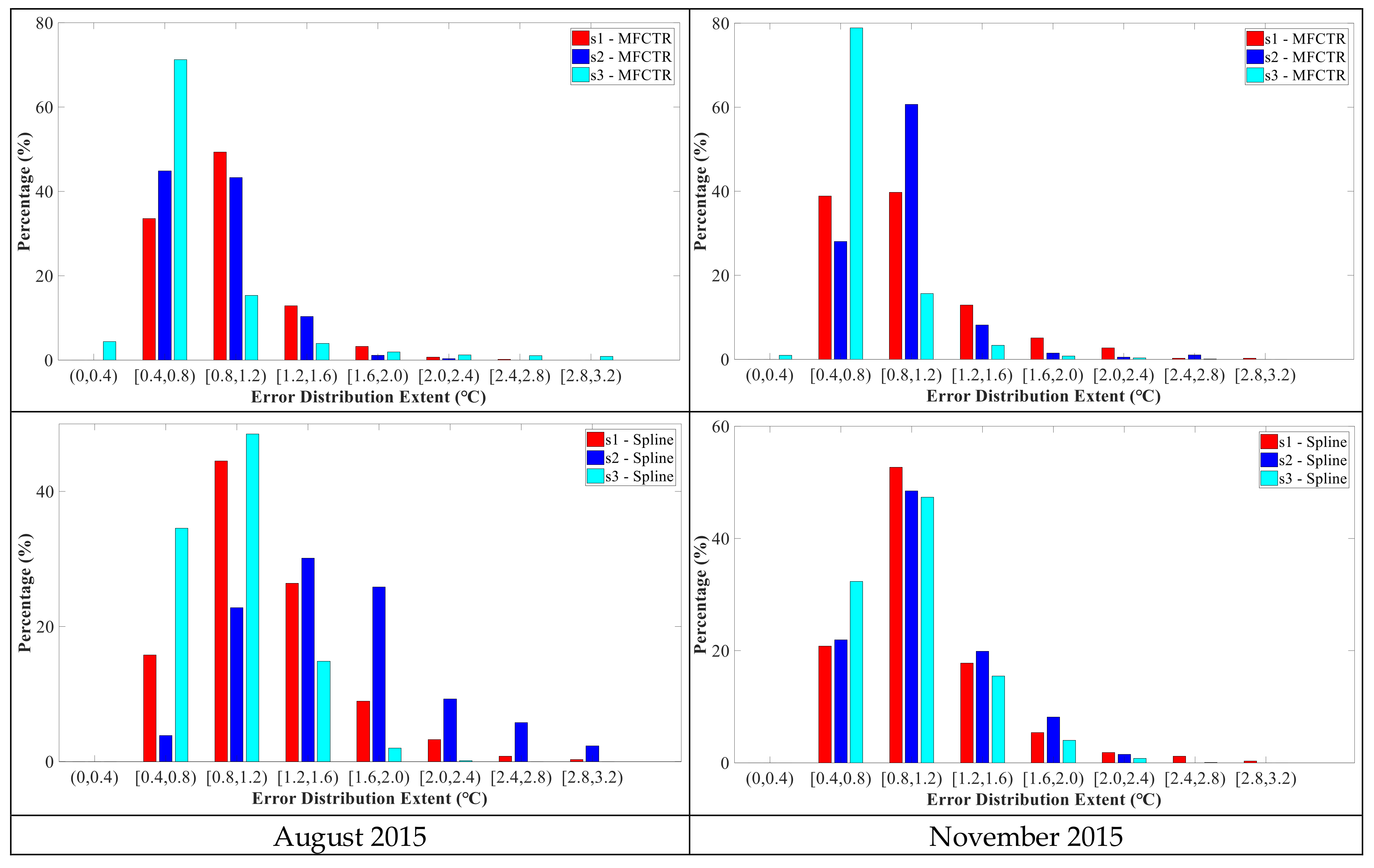
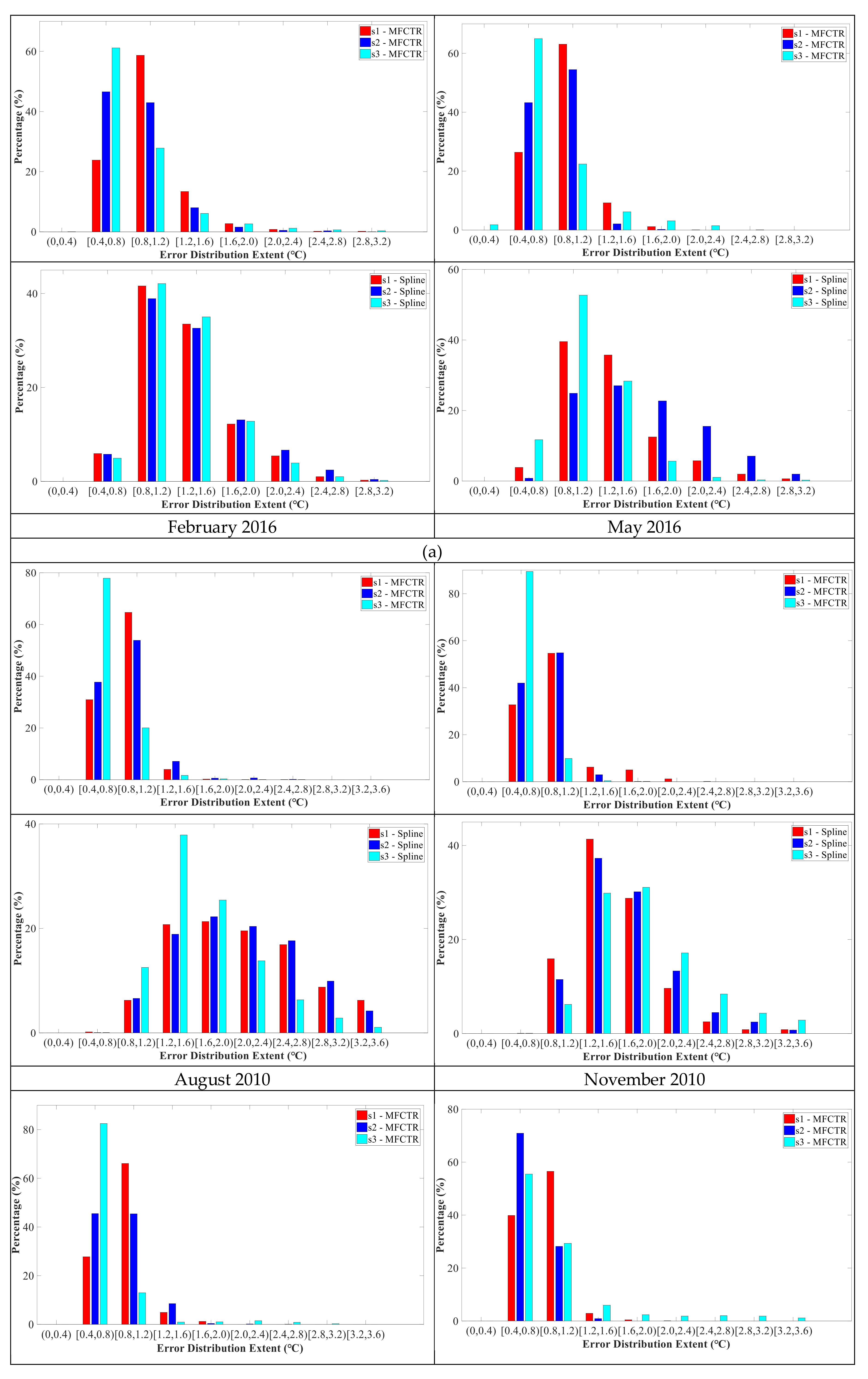
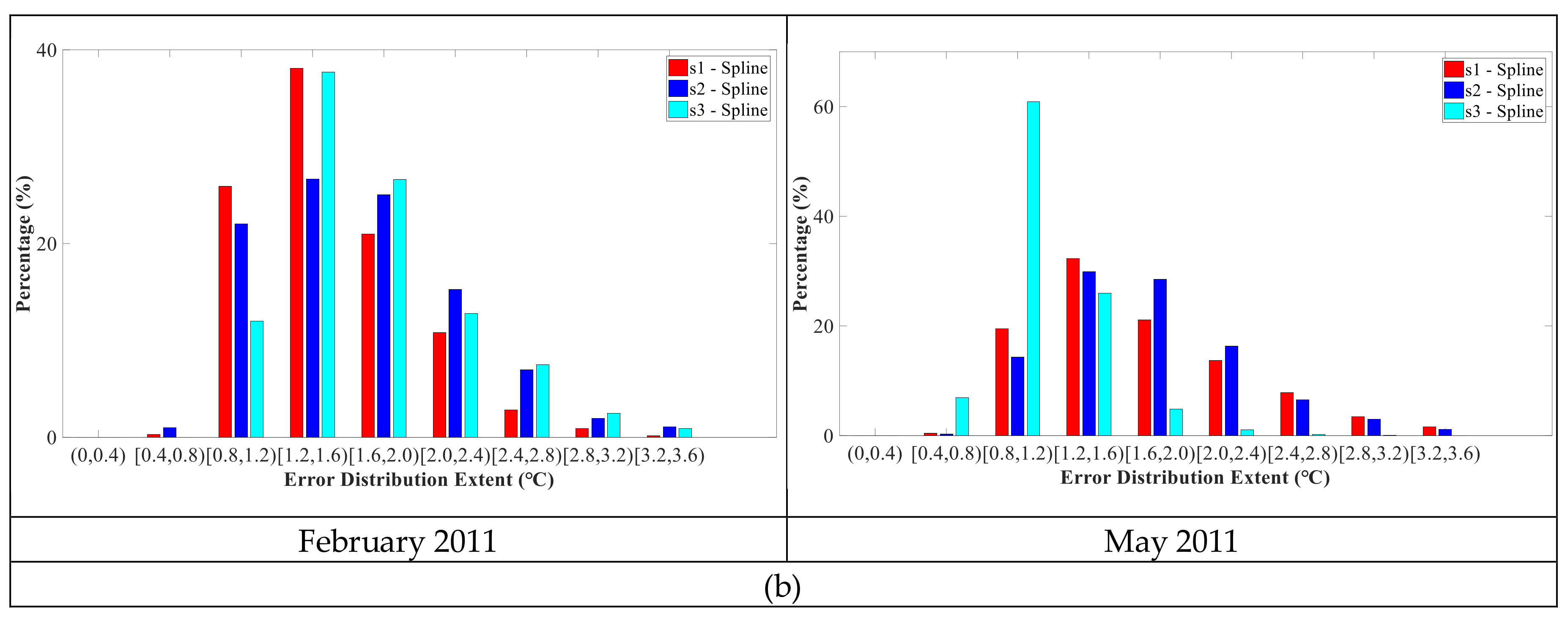
To better compare the error distribution of the two methods, we further carried out statistical analysis on the error of reconstructed LST images in the study areas. The resulting histograms are given in Figure 7. The errors for MFCTR-CNN were mostly concentrated in the 0.4 to 1.2 °C range for both FY-2G and MSG-SEVIRI. The errors for MFCTR-CNN in the night in the 0.4 to 0.8 °C range were mostly up to 60%. The distributions of errors for spline spatial interpolation were nearly normally distributed. The mean values of the normal distribution for FY-2G were approximately in the 0.8 to 1.2 °C range and about the 1.2 to 1.6 °C range for MSG-SEVIRI. For FY-2G, errors were distributed primarily under 3.2 °C, but the value is 3.6 °C for MSG-SEVIRI.

3.3.3. Application to Actual LST Data

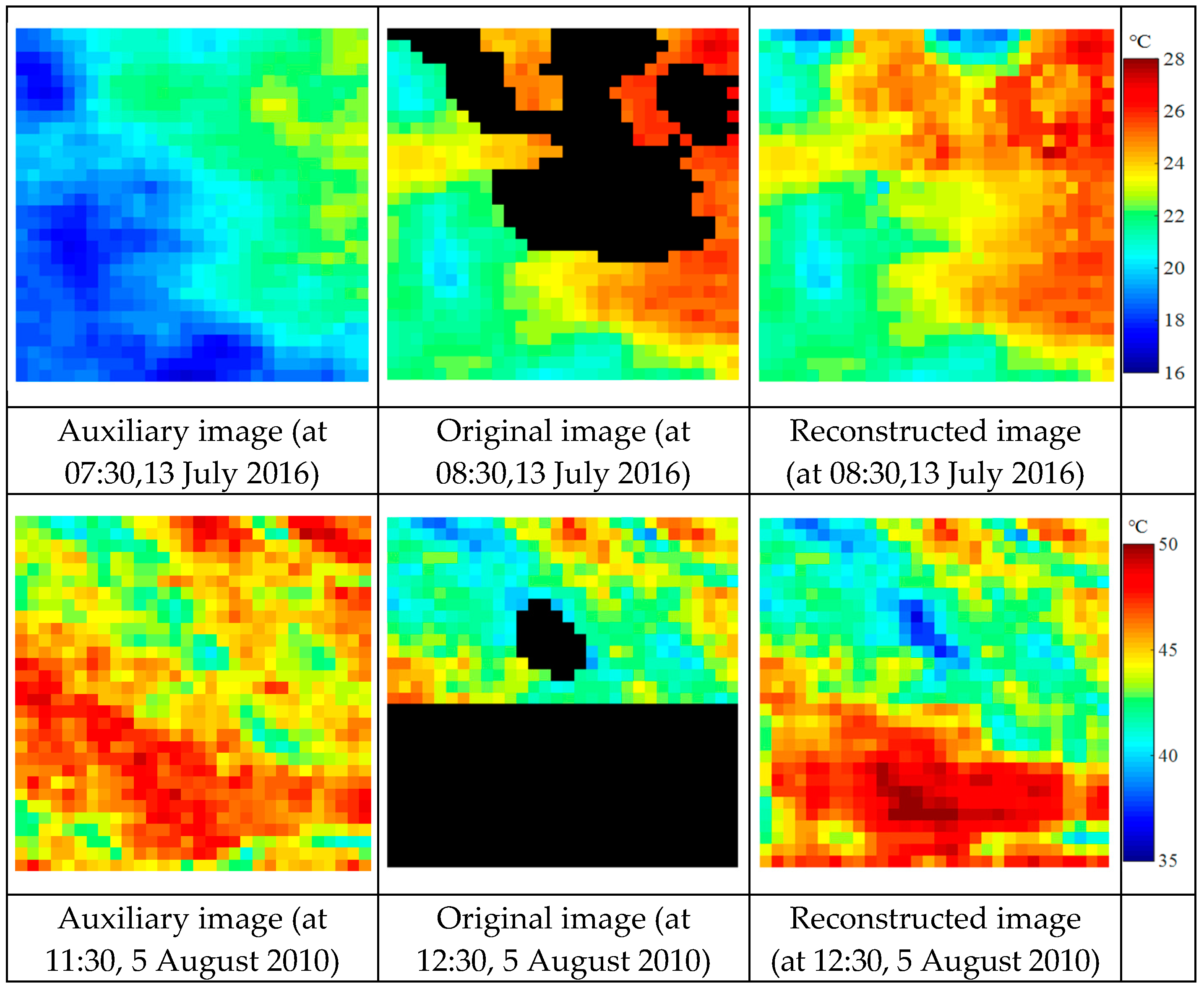
To verify the universality of the proposed model, the actual FY-2G LST (13 July 2016, 08:30) and MSG-SEVIRI LST (5 August 2010, 12:30) that originally contained many invalid pixels were selected. The reconstruction results are shown in Figure 8. Because the real LST values of the missing pixels were not obtained, a quantitative evaluation of the results cannot be performed. However, as seen from Figure 8, the reconstruction parts of the GLST images maintained good visual connectivity with the residual part, which proved again that the proposed model is feasible.

4. Discussion

Constructing remote sensing LST images is very important for their further applications in evaluating climate changes, monitoring urban heat islands, assessing ecosystem health, etc. Developing useful methods to fill LST images is essential. Inspired by the good performance of deep learning in solving highly dynamic and nonlinear problems, a MFCTR-CNN was proposed for recovering missing values in LST images. The effectiveness was elaborately examined and compared by using different satellites’ data in different seasons and different years with varied land-cover types. The classic spline spatial interpolation method was recommended as a comparison method. Generally, the proposed MFCTR-CNN could achieve better results. The RMSEs were mostly under 1 °C in different seasons with different missing data rates and different distribution characteristics of the missing observations (i.e., concentrated or scattered as in Figure 4). The results of the spline spatial interpolation method were strongly influenced by the missing data rate, and different distribution characteristics of the missing observations. The experiments show that the proposed MFCTR-CNN performed better in terms of both accuracy and reliability.

The key factor for the good performance of MFCTR-CNN is that it combined spatial and temporal information simultaneously. As stated above, existing LST image reconstruction methods do not simultaneously utilize spatial and temporal information of the data though, for some spatiotemporal methods, they may adopt one kind of information initially to recover some part of the invalid values, then use another to fill in the residual part. However, the correlation between the two kinds of information is probably important for reconstructing LST images. To better make use of spatial and temporal information, some specific structures (such as input combination and a spatial fusion unit) were applied to the network to ensure the network can mine the spatial and temporal information and the latent correlation between them. In addition, to relieve the burden of the GPU, the LST images were often clipped into small patches. However, some integrated structures may be broken with cutting, thus causing reconstructing errors, especially in patch margins. Therefore, an overlapped clipping strategy was employed in this article. The edge values would be covered by adjacent patches by using this approach. Furthermore, it was found that the overlapping size has an impact on reconstruction accuracy and, in the experiments, we found that the half size of the image patch is the best choice for overlapping. However, it should be stated that this may not be good for other tests. The best size of overlap must be found again in a new test.

However, it should be noted that there are several potential limitations to the proposed method. First, down-sampling and up-sampling architecture was applied in the proposed MFCTR-CNN, which used pooling layers to enlarge the receptive filed. For each pooling layer, the output LST image size is half of the input, and three pooling layers were applied in the down-sampling procedure of the proposed MFCTR-CNN. The size of LST image patches would become one eighth of the originals, so it is required that the size of the input LST image patches was a multiple of eight, such as 16, 32, 40, etc. Additionally, 2D convolution in the convolution network needs the input LST image patches to have equal height and width. In the proposed MFCTR-CNN, the ancillary LST image patches must not contain invalid pixels. Considering the above requirements of the input LST image patch size, it is difficult to generate enough data in some situations. Some more optimized deep learning networks should be designed to relax the restricted conditions on the size of input LST image patches. Moreover, a few outliers with high error in the filled results can be found where these pixels have few similar training samples. This is an inherent problem in convolution networks, which perform badly when the training data are insufficient. It is therefore necessary to evaluate whether the training samples are representative or not. Finally, as in previous LST reconstruction methods [7,8,10,13,14,18], the reconstructed LST values of the proposed method are estimated under cloud-free conditions. However, the missing data are mostly pixels covered by clouds when deriving LST from satellite data. The actual LST values of cloud-covering pixels should be lower or higher than the reconstructed LST values in daytime or nighttime. Although most of these algorithms were specifically developed for clear sky conditions, the reconstructed values are also meaningful for research on climate, agriculture, and ecology. In adding passive microwave data or in situ measurements as training samples [40], it is possible to estimate the LST under an actual cloudy situation using the proposed MFCTR-CNN, which will also be addressed in our future work.

5. Conclusions

In this paper, a fully convolutional network with multiscale feature connected architecture was proposed for reconstructing geostationary satellite LSTs with large missing regions. In order to establish the highly dynamic nonlinear relationship among GLSTs, different temporal inputs were added and concatenated. In addition, multiscale features were connected by using a spatial attention unit to better retain the useful position information of LSTs. Finally, average pooling was applied to build the relationship of LSTs with large missing regions. Compared with traditional reconstruction methods, the proposed MFCTR-CNN shows a better performance with varied land-cover types from different satellites and different seasons. Although MFCTR-CNN was tested with LST in this study, it provides a new framework and advances capabilities for reconstructing other remotely sensed data products with spatiotemporal dynamics. Such a capability will be beneficial for monitoring land-surface and ecological dynamics.